


1. Introduction
A jet in crossflow describes a common flow configuration, where a (reactive or non-reactive) jet exits perpendicularly from an orifice into a transverse boundary layer, producing a complex three-dimensional flow that exhibits a wide range of instabilities and sustained flow characteristics. This flow configuration is considered prototypical as it features in many engineering applications such as in fuel injection systems, in dilution holes in gas turbines, in film cooling devices for turbomachinery, in control actuators for boundary layer separation and – perhaps most prominently – in smoke stacks. Not surprisingly then, jets in crossflow have been the subject of numerous experimental and numerical studies (Meyer, Pedersen & Özcan Reference Meyer, Pedersen and Özcan2007; Karagozian Reference Karagozian2010; Mahesh Reference Mahesh2013; Karagozian Reference Karagozian2014), and a detailed review of the principal flow structures is given in Kelso, Lim & Perry (Reference Kelso, Lim and Perry1996). As the exiting jet gradually bends in the crossflow, a counter-rotating vortex pair forms which further entrains the crossflow. Moreover, the shear layer along the upstream edge of the jet supports oscillations that amplify, roll up, advect along the curved jet axis and eventually lead to breakdown of the flow into turbulent fluid motion.
As a key parameter, the jet-to-crossflow velocity ratio  $R$ has been identified: for low values of
  $R$, the flow in the near field is strongly accelerated, affecting the trajectory of the jet, its entrainment and eventual mixing behaviour; for high values of
  $R$, the emergence of coherent structures is responsible for the bulk of the crossflow entrainment, yielding a far less efficient mixing behaviour in the near field. Besides these qualitative differences, the jet-to-crossflow ratio also affects the nature of the dominant instability. For high values of
  $R$, a convectively unstable behaviour is observed (Karagozian Reference Karagozian2014), which changes to an absolutely unstable behaviour as
  $R$ is lowered. This bifurcation is also reflected in the vorticity evolution in the shear layer, resulting in distinct flow patterns in either parameter regime.
Due to the three-dimensionality of the flow, a global stability analysis is the most appropriate approach for studying the instability characteristics of a jet in crossflow and for extracting the unstable modes Huerre (Reference Huerre2007). Applying this method to a jet with  $R=3$, Bagheri et al. (Reference Bagheri, Schlatter, Schmid and Henningson2009) found high-frequency unstable global eigenmodes associated with shear-layer instabilities on the counter-rotating vortex pair and low-frequency modes associated with shedding vortices in the wake of the jet, suggesting an overall globally unstable jet. Ilak et al. (Reference Ilak, Schlatter, Bagheri and Henningson2012) also analysed the jet for increasing
  $R$ and showed that the flow changes from a simple periodic vortex shedding to a more complex quasi-periodic behaviour, before rapidly breaking down into turbulence. At lower values of
  $R$, global linear stability analysis predicts well the dominant frequency and the initial growth rate of the nonlinear flow. At higher values of
  $R$, however, multiple unstable eigenmodes arise, resulting in a more complicated flow behaviour. The same study also identified the spatial origin of the first instability in the shear layer immediately downstream of the jet. This was confirmed more recently by a global linear stability analysis (Regan & Mahesh Reference Regan and Mahesh2017), matching the observations reported in Megerian et al. (Reference Megerian, Davitian, Alves and Karagozian2007), where the upstream shear layer undergoes a transition from absolute to convective instability in the interval from
  $R=2$ to
  $R=4$.
Linear stability analyses are restricted to the perturbation dynamics about a laminar state, which often exclude parameter regimes of interest in industrial settings. Other data decomposition techniques, such as proper orthogonal decomposition (Rowley Reference Rowley2005) or dynamic mode decomposition (Schmid Reference Schmid2010; Tu et al. Reference Tu, Rowley, Luchtenburg, Brunton and Kutz2014), are suitable alternatives, allowing a modal breakdown of such flows into coherent structures and their temporal dynamics. Using nonlinear direct numerical simulations together with a modal decomposition (proper orthogonal decomposition), Schlatter, Bagheri & Henningson (Reference Schlatter, Bagheri and Henningson2011) analysed the stability of a configuration similar to that of Bagheri et al. (Reference Bagheri, Schlatter, Schmid and Henningson2009), demonstrating the presence of self-sustained periodic oscillations, even in the absence of external forcing. Iyer & Mahesh (Reference Iyer and Mahesh2016) also confirmed these results using a dynamic mode decomposition approach.
While the jet-to-crossflow velocity ratio is undoubtedly an important factor in determining the nature of instabilities in such flow configurations, the impact of reactions, and in particular the resulting heat release, is also non-negligible. Heat release in the reaction zone has been shown to impact the development and evolution of shear-layer vortices (Lyra et al. Reference Lyra, Wilde, Kolla, Seitzman, Lieuwen and Chen2015; Pinchak, Shaw & Gutmark Reference Pinchak, Shaw and Gutmark2019; Nair et al. Reference Nair, Wilde, Emerson and Lieuwen2019b). In particular, Chen et al. (Reference Chen, Roquemore Wrdci, Goss and Vilimpoc1991) have demonstrated that the flame structure in a mixture fraction space plays an important role in the generation or destruction of such vortical structures. In addition, the presence of reactions has been shown to have an impact even on steady-state flow structures (Nair et al. Reference Nair, Sirignano, Emerson, Halls, Jiang, Felver, Roy, Gord and Lieuwen2019a). A similar analysis, using data-driven techniques, has also shown dramatic differences in the shape of the extracted modes (Sayadi et al. Reference Sayadi, Lyra, Hamman, Kolla, Schmid and Chen2015), highlighting the large impact of combustion on the dynamics of the jet and motivating the present study.
The presence of different stability characteristics has a significant effect on the manner by which optimal external excitation can be used to control jet penetration and spread (Karagozian Reference Karagozian2014). Experimental studies of a forced jet with  $R=6$, using a single-frequency actuator, have shown a strong receptivity of the jet inlet to high-frequency forcing, which is expected due to the convectively unstable nature of the jet in this parameter regime. For lower-frequency forcings, the jet was responsive further downstream where counter-rotating vortices are active (Narayanan, Barooah & Cohen Reference Narayanan, Barooah and Cohen2003). With this variety of response behaviour and the realization that reactions can have a substantial influence on the instability mechanisms, a detailed analysis spanning various forcing frequencies and jet-to-crossflow ratios
  $R$ in both the reactive and non-reactive regimes is necessary to fully describe and map out the frequency response characteristics of a jet in crossflow. For the purpose of this study, our focus is directed towards a case with
  $R = 3$, resulting in a globally unstable jet, and the response of both reactive and non-reactive jets is extracted as the forcing frequency is varied. The optimal forcing and response solutions are determined using an adjoint-based methodology and compared for both regimes.
An adjoint-based analysis is particularly suited for our undertaking as it casts the search for a response to external forcing into an optimization problem that determines the maximum energy gain a linearized system can experience as it maps an input forcing to an output reaction. Originally arising in design optimization for fluid systems (e.g. Pironneau Reference Pironneau1974; Jameson Reference Jameson1988; Jameson, Martinelli & Pierce Reference Jameson, Martinelli and Pierce1998; Reuther et al. Reference Reuther, Jameson, Alonso, Rimlinger and Saunders1999), adjoint methods have established themselves as key tools in the stability, receptivity and sensitivity analysis of fluid systems, for example, for aero- and thermo-acoustic applications (e.g. Juniper Reference Juniper2010; Lemke, Reiss & Sesterhenn Reference Lemke, Reiss and Sesterhenn2013). These application areas provide a suitable application for adjoint-based methods, as they are dominated by a mostly linear dynamics. Extensions to nonlinear systems have allowed the analysis of high-lift airfoils, mixing enhancement and minimal seeds for transition to turbulence (Schmidt et al. Reference Schmidt, Ilic, Schulz and Gauger2013; Foures, Caulfield & Schmid Reference Foures, Caulfield and Schmid2014; Rabin, Caulfield & Kerswell Reference Rabin, Caulfield and Kerswell2014; Eggl & Schmid Reference Eggl and Schmid2020), among many other applications. Recently, the same techniques have also been applied to reactive flows, either by aiding the adaptive mesh refinement in steady-state Reynolds-averaged Navier–Stokes calculations (Duraisamy & Alonso Reference Duraisamy and Alonso2012), or in detailed simulations of one- and two-dimensional laminar configurations with decoupled reactive equations (Braman, Oliver & Raman Reference Braman, Oliver and Raman2015). The parametric sensitivity in solid-particle combustion has been addressed in Hassan et al. (Reference Hassan, Sayadi, LeChenadec, Pitsch and Attili2020) and standard premixed flames based on simplified combustion models (Blanchard et al. Reference Blanchard, Schuller, Sipp and Schmid2015; Sashittal et al. Reference Sashittal, Sayadi, Schmid, Jang and Magri2016; Capecelatro, Bodony & Freund Reference Capecelatro, Bodony and Freund2017; Skene & Schmid Reference Skene and Schmid2019). In all these applications, the adjoint methodology exploits the high dimensionality of the input space to provide general gradient measures that can be used to improve performance, extract highly observable structures or quantify robustness or sensitivity with respect to parameter changes. We employ the same technology to determine the response behaviour of a jet in crossflow and study the commonalities and differences between non-reacting and reacting cases.
The paper is structured as follows. Section 2 presents the equations governing the flow and reactive chemistry, together with the appropriate boundary conditions. The adjoint equations are presented in § 3, along with the linearized form of the governing equations and forcing function. Section 4 then contains concise information on the numerical method used to discretize and solve the resulting nonlinear/linear governing equations as well as the adjoint problem. The results of our analysis are described in § 5, followed by a summary and conclusions in § 6.
2. Governing equations
The flow is governed by the compressible reactive Navier–Stokes equations. In the reactive case, the Lewis number  $Le$ of all species is taken as unity and, for simplicity, the heat capacity is assumed to be constant. The scalar diffusion is modelled by Fick's law, resulting in the following system of equations:
 $$\begin{gather} \frac{\partial \rho}{\partial t} + \frac{\partial}{\partial x_j}(\rho u_j) = 0, \end{gather}$$
 $$\begin{gather}\frac{\partial \rho u_i}{\partial t} + \frac{\partial}{\partial x_j}(\rho u_i u_j + p\delta_{ij}) = \frac{\partial \sigma_{ij}}{\partial x_j}, \end{gather}$$
 $$\begin{gather}\frac{\partial E}{\partial t} + \frac{\partial}{\partial x_j}[(E+p)u_j] = \dot{\omega}_T-\frac{\partial q_j}{\partial x_j} + \frac{\partial}{\partial x_j}(u_k\sigma_{jk}), \end{gather}$$
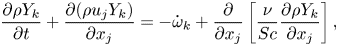 $$\begin{gather}\frac{\partial \rho Y_k}{\partial t} + \frac{\partial ( \rho u_j Y_k)}{\partial x_j} ={-}\dot{\omega}_k + \frac{\partial}{\partial x_j}\left[\frac{\nu}{Sc}\frac{\partial \rho Y_k}{\partial x_j}\right], \end{gather}$$
where
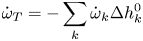 \begin{equation} \dot{\omega}_T ={-}\sum_k \dot{\omega}_k \Delta h^{0}_{k} \end{equation}
and  $\rho , u_i, p, E, \sigma _{ij}$ and
  $q_i$ are the non-dimensional density, velocity components, pressure, total energy, viscous stress tensor and heat flux, respectively. The parameter
  $\nu$ stands for the kinematic viscosity and
  $Sc$ represents the Schmidt number, which is set to
  $0.7$ in this study. Parameter
  $Y_k$ denotes the mass fraction of each species, and
  $\dot {\omega }_k$ stands for the production rate of species
  $k$, where
  $\Delta h^{0}_{k}$ is the respective heat of formation at some reference temperature
  $T_0$. In our case, only the fuel mass fraction is explicitly computed,
  $k=1$, and
  $Y_k = Y_f$, assuming lean reaction. The above set of equations is closed using the equation of state:
 \begin{equation} p = \dfrac{\mathcal{R}}{W}\rho T, \end{equation}
where  $\mathcal {R}$ is the universal gas constant and
  $W$ is the mean molecular weight of the mixture, describing the properties of a perfect gas.
2.1. Chemistry
A simple one-step chemistry model is used for evaluating reactive source terms. The fuel mass reaction rate is given by the Arrhenius law of the form
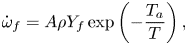 \begin{equation} \dot{\omega}_f = A \rho Y_f \exp\left(-\frac{T_a}{T}\right), \end{equation}
where  $A$ is the Arrhenius pre-exponential factor and
  $T_a$ is the activation temperature. Assuming constant specific heat ratio, and unity Lewis number, the combustion source terms, the fuel mass depletion rate
  $\dot {\omega }_f$ and the reaction heat release rate
  $\dot {\omega }_T$, all in the non-dimensional form, are given as
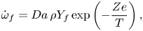 $$\begin{gather} \dot{\omega}_f = Da \, \rho Y_f \exp \left( -\frac{Ze}{T} \right), \end{gather}$$
 $$\begin{gather}\dot{\omega}_T = Q \, \dot{\omega}_f. \end{gather}$$
The combustion parameters used in the source terms are described by the following non-dimensional numbers: the Damköhler number  $Da$, the Zeldovich number
  $Ze$ and the heat release parameter
  $Q$. For this study, we have chosen
  $Da = 10$,
  $Ze = 5$ and
  $Q = 10$. These parameters are similar to those for the case presented in Blanchard et al. (Reference Blanchard, Schuller, Sipp and Schmid2015) for an
  ${\boldsymbol{\mathsf{M}}}$-flame, which produces verifiable results using a matching experimental configuration. In the case of the jet, on the other hand, these parameters yield reactions far weaker than those of existing experiments and numerical simulations (Mahesh Reference Mahesh2013; Karagozian Reference Karagozian2014). Most available configurations of a reactive jet in crossflow are based on a turbulent inlet and jet flow. In contrast, we aim to compare the jets in the laminar regime, where instability results of the cold case can be validated against existing theoretical analysis, and thus consider a laminar inlet and jet, motivating the parameters chosen above. The resulting state vector considered in this study is given as
 \begin{equation} {\boldsymbol{q}} = [ \rho\quad \rho u_1 \quad\rho u_2\quad \rho u_3\quad E\quad \rho Y_f]^{\top}, \end{equation}
where  $\rho$ is the density,
  $u_i$ is the velocity component in the
  $i$th coordinate direction,
  $E$ is the total energy and
  $Y_f$ is the mass fraction of the fuel.
2.2. Boundary conditions
The velocity profile inside the jet inlet is prescribed using an inhomogeneous boundary condition, through the wall-normal velocity at the wall of the plate, similar to Bagheri et al. (Reference Bagheri, Schlatter, Schmid and Henningson2009). Direct numerical simulations of the transverse jet demonstrate that, for jet-to-free-stream velocity ratios of  $R \geqslant 3$, the flow characteristics are faithfully reproduced. Owing to the compressible setting, we need to impose the temperature profile inside the jet inlet as well. Similar to the velocity profile, a bi-quadratic profile with a maximum of
  $T_{{jet}} = Pr V_{{jet}}^{2}/4,$ above the wall temperature, is imposed, resulting in
 \begin{equation} T(r) = T_w + T_{{jet}}(1-r^{4}) \exp\left( -(r/0.7)^{4} \right), \end{equation}
where  $r$ denotes the distance from the jet centre, normalized by half the jet diameter,
  $T_w$ is the wall temperature,
  $Pr = 0.7$ is the Prandtl number and
  $V_{{jet}}$ and
  $T_{{jet}}$ represent jet velocity and temperature, respectively. The temperature profile is rendered smooth by a super-Gaussian function, such that the derivatives remain continuous across the jet. In the reactive case, the concentration of fuel is set to one inside the jet and to zero in the crossflow.
Periodic boundary conditions are used in the spanwise and streamwise coordinate directions. To account for the spatially growing boundary layer in a streamwise-periodic domain, we reshape and rescale the profile at the end of the computational domain into the similarity solution of a laminar compressible boundary layer at the inflow. This reshaping procedure is performed inside a sponge region, following Spalart & Watmuff (Reference Spalart and Watmuff1993). Within all sponge zones, which are placed at the top, inlet and outlet of the computational domain, the similarity solution of the compressible laminar boundary layer is prescribed.
3. Adjoint-based framework
Our analysis utilizes a computational optimization framework to extract the dominant structures responsible for the bulk of the energy transport in the jet in crossflow. This framework relies on a variational formulation using adjoint equations or Lagrange multipliers.
The derivation of adjoint equations can be carried out in two fundamental ways. In the continuous approach, the first variation of an augmented cost functional yields governing equations for the adjoint variables with appropriate boundary conditions and initial conditions. These equations together with the original governing equations are then properly discretized and implemented. For governing equations of even moderate complexity, this process is rather cumbersome and error-prone. Alternatively, the spatially discretized equations can be furnished to automatic differentiation software to produce an associated adjoint code. This process, although straightforward to execute, can lead to overly inflated, and ultimately impractical, code. As a compromise, we employ the approach outlined in Fosas de Pando, Sipp & Schmid (Reference Fosas de Pando, Sipp and Schmid2012). The discrete adjoint operators are obtained by taking the conjugate transpose of the discretized direct operator in a modular way, thus yielding an adjoint code of complexity comparable to that of the original code. This approach has been used to analyse acoustic feedback phenomena (Fosas de Pando et al. Reference Fosas de Pando, Sipp and Schmid2012) and the stability properties of an axisymmetric  $\boldsymbol{\mathsf{M}}$-flame (Blanchard et al. Reference Blanchard, Schuller, Sipp and Schmid2015).
We consider the response of a jet in crossflow to harmonic forcing and seek to identify a particular forcing shape that maximizes a specified energy gain over a given time horizon. Adopting a general formulation, the forward/direct equation constitutes the evolution of the state variable  $\boldsymbol {q}$ in time defined by
 \begin{equation} \frac{\textrm{d}\boldsymbol{q}}{\textrm{d}t} = \boldsymbol{\mathsf{A}} {\boldsymbol{q}} + \boldsymbol{\mathsf{B}} {\boldsymbol{g}}(\boldsymbol{f}) \sin(2{\rm \pi}\omega t) = {\boldsymbol{R}}(\boldsymbol{q},\boldsymbol{f},\omega), \quad\boldsymbol{q}(0) = 0, \end{equation}
where  $\boldsymbol{\mathsf{A}} = \partial \boldsymbol {F} / \partial \boldsymbol {q} |_{\bar {\boldsymbol {q}}}$ with
  $\boldsymbol {F}$ representing the discrete nonlinear equations that govern the evolution of the state variables and
  $\bar {\boldsymbol {q}}$ denoting the base flow. The matrix
  $\boldsymbol{\mathsf{B}}$ is a masking matrix, used to select the area in the domain where the forcing function
  ${\boldsymbol {f}}$ is active. It should be noted that
  $\boldsymbol{\mathsf{B}}$ does not specify the form of the forcing solution; the matrix is merely used to ensure that the forcing function is suppressed in irrelevant regions of the flow, such as the sponge regions. It is also chosen to enforce an identical spatial forcing distribution in both the reactive and non-reactive case and thus allow a fair comparison. In this study, the non-conservative variables are forced; therefore, the forcing vector
  ${\boldsymbol {f}}$ can be defined as
  $[f_\rho , f_u, f_v, f_w, f_{{Temp}}, f_Y]$. For simplicity, the energy is not directly forced, resulting in
  $f_{{Temp}} = 0.$ However, since the equations are solved for conservative state variables, the forcing term has to be transformed accordingly from non-conservative to conservative form. This is accomplished by the function
  ${\boldsymbol {g}}(\boldsymbol {f}).$ The linearized system is forced at a frequency
  $\omega$.
The cost functional  ${\mathcal {J}}$ can then be formulated as
 \begin{equation} {\mathcal{J}}(\boldsymbol{q}) = \phi(\boldsymbol{q}(T_f),\boldsymbol{f}) + \int_0^{T_f} \psi(\boldsymbol{q}(t),\boldsymbol{f})\,\textrm{d}t, \end{equation}
where  $\phi$ is the contribution from the terminal state to the cost functional at final time
  $T_f$,
  $\boldsymbol {f}$ represents the shape of the forcing function and
  $\psi$ accounts for an integral contribution to the cost functional. Using this cost functional, the augmented Lagrangian
  ${\mathcal {L}}$ can be stated as
 \begin{equation} {\mathcal{L}}(\boldsymbol{q},\boldsymbol{f},\boldsymbol{\eta},\xi; \omega) = {\mathcal{J}}(\boldsymbol{q}) - \int_0^{T_f} \boldsymbol{\eta} \boldsymbol{\cdot} \left( \dfrac{\textrm{d}\boldsymbol{q}}{\textrm{d}t} - {\boldsymbol{R}}(\boldsymbol{q},\boldsymbol{f},\omega)\right) \textrm{d}t -\xi(\boldsymbol{f}\boldsymbol{\cdot}\boldsymbol{f} - 1). \end{equation}
To proceed, we introduce a scalar product (and an associated norm) in the form  $\langle \boldsymbol {u, v} \rangle = \boldsymbol {v}^{\top } {\boldsymbol{\mathsf{Q}}} \boldsymbol {u}.$ The matrix
  $\boldsymbol{\mathsf{Q}}$ represents a symmetric positive-definite mass matrix that accounts for the volume integral over the discretized domain. To simplify our analysis, we choose
  $\phi (\boldsymbol {q}(T_f),\boldsymbol {f}) = \langle \boldsymbol {q}(T_f), \boldsymbol {q}(T_f)\rangle /\langle \boldsymbol {f}, \boldsymbol {f}\rangle$ and
  $\psi (\boldsymbol {q}(t),\boldsymbol {f}) = 0$.
Mathematically, we can accommodate different norms for the forcing and the response. Moreover, only the measure for  $\boldsymbol {f}$ must be a real norm; the measure for the response can be a semi-norm and thus contain only a subset of the state vector components. The choice of norm will produce quantitative differences, but, within reasonable bounds, norms that account for all relevant state vector variables will yield qualitatively similar outcomes and coherent structures. For compressible flows, a common option is the Chu norm (Chu Reference Chu1965; Hanifi, Schmid & Henningson Reference Hanifi, Schmid and Henningson1996) which can be derived under the assumption of vanishing compression work. In our case, this choice does not present a viable option, since we expect important pressure contributions stemming from reactive effects. For this reason, we adopt a straightforward Euclidean
  $L_2$-norm that accounts for all state vector components equally, for both the forcing and the response. For the non-reactive case, this entails the inclusion of the passive scalar – a step that also allows a fair comparison between reactive and non-reactive cases. It is, however, important to stress that the inclusion of the passive scalar for the non-reactive case does not lead to unphysical effects, since the passive scalar, by its nature, cannot instigate instabilities or be otherwise responsible for amplification effects. In summary, we base our analysis on a Euclidean norm that takes into account all dynamic state vector components, including density, momentum and energy terms together with passive scalars (for the non-reacting case) or mass fractions for each species (for the reactive case).
With the scalar product and norm established, we set the first variation of the augmented Lagrangian  ${\mathcal {L}}$ with respect to the state variables
  ${\boldsymbol {q}}$ to zero, which leads to the adjoint equations and a terminal condition, defined by
 \begin{equation} -\dfrac{\textrm{d}\boldsymbol{\eta}}{\textrm{d}t} = \left( \dfrac{\partial {\boldsymbol{R}}}{\partial \boldsymbol{q}}\right)^{\top} \boldsymbol{\eta}, \quad \boldsymbol{\eta}(T_f) = 2{\boldsymbol{\mathsf{Q}}}\boldsymbol{q}(T_f)/\langle \boldsymbol{f}, \boldsymbol{f}\rangle. \end{equation}
It can be deduced from (3.4a,b) that the equation governing the evolution of the adjoint variable is initialized by the terminal solution of the direct system  $\boldsymbol {q}(T_f)$. The optimality condition is given by rendering zero the first variation of
  ${\mathcal {L}}$ with respect to the forcing function, yielding an expression for the optimal forcing
  ${\boldsymbol {f}}$ of the form
 \begin{equation} \boldsymbol{f} = \dfrac{1}{2\xi} \int_0^{T_f} \left(\boldsymbol{\mathsf{B}}\dfrac{\partial {\boldsymbol{g}}(\boldsymbol{f})}{\partial \boldsymbol{f}}\right)^{\top} \boldsymbol{\eta} \sin(2{\rm \pi}\omega t) \,\textrm{d}t \end{equation}
with  $\xi$ as a normalizing constant for
  $\boldsymbol {f}$. Solving the adjoint equations together with the constraints in one step is computationally expensive. For this reason, an iterative approach is adopted, whereby a conjugate-gradient algorithm with line search is employed, and
  ${\boldsymbol {f}}$ is updated repeatedly using the gradient computed from (3.5). In addition, since the goal of this study is to determine the frequency response of the system for a range of forcing frequencies, the gradient of the cost functional with respect to the forcing frequency
  $\omega$ is used, which can be easily obtained by differentiating the Lagrangian
  ${\mathcal {L}}$ with respect to
  $\omega .$ This results in
 \begin{equation} \dfrac{\partial {\mathcal{L}}}{\partial \omega} = \int_0^{T_f} \omega \boldsymbol{\mathsf{B}} {\boldsymbol{g}}(\boldsymbol{f}) \cos(2{\rm \pi}\omega t) \, \textrm{d}t. \end{equation}
This gradient can be used to represent the frequency response curve more accurately via cubic Hermite interpolation in the frequency.
It is important to stress that a gain optimization over a specified time horizon  $T_f$ is distinct from a resolvent analysis of the flow. The latter analysis considers the asymptotic limit of
  $T_f\to \infty$ and presents the steady-state harmonic response to a time-periodic forcing at a given frequency, after possible transient effects have subsided. In our case, we study the frequency response of the flow over a finite time interval
  $[0, T_f]$ that is attuned to a characteristic time scale of the flow. Coherent structures that are optimal in gain over this temporal window are assumed to prevail in the flow and be responsible for the presence of observable flow patterns. Especially in the presence of combustion, a more narrow time window, over which harmonic perturbations from an ambient disturbance environment are amplified, is preferable.
4. Numerical details
Direct numerical simulations of non-reactive and reactive jets in crossflow are performed using a modified version of the solver developed by Nagarajan, Lele & Ferziger (Reference Nagarajan, Lele and Ferziger2003) and Sayadi, Hamman & Moin (Reference Sayadi, Hamman and Moin2013). Fourth-order finite differences are used to discretize the three spatial coordinate directions. The numerical scheme is formulated on a structured curvilinear grid, and the variables are staggered in space. Operator splitting is employed to advance the state variables in time: an explicit third-order low-storage Runge–Kutta method is used for integrating the flow variables, followed by a fifth-order backward differentiation method (Brown, Byrne & Hindmarsh Reference Brown, Byrne and Hindmarsh1989) for advancing the reaction variables.
The computational domain is similar to the configuration in Bagheri et al. (Reference Bagheri, Schlatter, Schmid and Henningson2009). The free-stream Mach number is set to  $Ma = 0.2$. The jet-to-freestream velocity ratio is
  $R = 3$, resulting in a Mach number of
  $0.6$ at the jet inlet. The reference Reynolds number, based on the distance from the leading edge, is
  $Re_{{ref}} = 10^{4},$ and the reference distance
  $x_{ref}$ is taken as the distance of the inlet station from the leading edge, so that
  $x/x_{{ref}} = Re_x/10^{4}.$ The inlet of the computational domain is at
  $x_{{inlet}} = 0.7$, and the jet centreline is placed in the mid-spanwise plane
  $z = 0.15$ and at a streamwise distance of
  $0.92$ from the leading edge. The diameter of the jet is
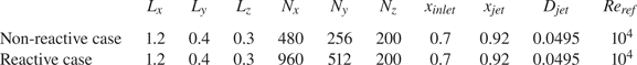
  $D_{{jet}} = 0.0495$. Further details of the computational domain are given in table 1. Note that the grid in the reactive case is twice as resolved in the streamwise and wall-normal directions. The higher resolution is required to properly capture the dynamics of the flame.
Table 1. Details of the computational domain.
5. Results
In this section, results of the reactive and non-reactive jet in crossflow are presented and compared. First, the flow fields from the nonlinear simulations are analysed, and the coherent structures of the two jets are compared. Using data decomposition techniques, the dominant frequencies of each case are extracted, which define the range over which a subsequent linear analysis is performed. Differences in the steady base flow are investigated as well. Finally, an optimal frequency response for the identified nonlinear key frequencies is computed and compared for the reactive and non-reactive cases.
5.1. Nonlinear simulations
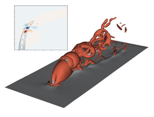
Figures 1(a) and 1(b) juxtapose instantaneous snapshots of vortical structures for the reactive and non-reactive cases. The visualization presents isosurfaces of the second invariant of the strain tensor  $Q$ (Hunt, Wray & Moin Reference Hunt, Wray and Moin1988, p. 193). Already the shape of the vortical structures indicates a noticeable change in the flow field when chemical reactions are present. The jet developing in the cold case breaks down earlier than in the reactive case, penetrating farther in the wall-normal direction despite identical jet-to-crossflow ratios. In addition, past the instability-induced breakup of the jet, the resulting structures downstream of the cold jet show smaller scales, compared to the reactive jet, suggesting an instability that acts at smaller wavelengths. Analysing the mass fraction (a passive scalar field in the reactive case) shows that the flame extinguishes before the breakdown of the jet occurs, resulting in an oscillating but ‘non-turbulent’ flame, which will play a significant role in our subsequent analysis.

Figure 1. (a,b) Isosurfaces of the  $Q$-criterion as an indicator of vortical structures in the instantaneous flow field. The grey contours depict the streamwise velocity component. (c) The instantaneous scalar field, presented by using volume rendering of the fuel mass density. High values of mass density are coloured in red, lower values in yellow. (a) Non-reactive jet in crossflow. (b) Reactive jet in crossflow. (c) Reacting scalar field.
Dynamic mode decomposition is used to extract coherent structures with a single temporal frequency from a sequence of data snapshots (Schmid Reference Schmid2010) in both the reactive and non-reactive cases. Previous studies have shown that the fundamental frequencies, pertaining to self-sustained oscillations in the flow, are linked to the region near the inlet of the jet (Schlatter et al. Reference Schlatter, Bagheri and Henningson2011). We thus limit our snapshot samples for both cases to the region near the inlet. This region comprises the shear layer upstream of the jet inlet and the separation region behind the inlet, i.e. in the wake of the jet. In order to objectively identify the most influential modes in the flow, a sparsity-promoting dynamic mode decomposition algorithm is employed (Jovanovic, Schmid & Nichols Reference Jovanovic, Schmid and Nichols2014). The dominant frequencies will help select the frequency ranges for our subsequent frequency response analysis.
Figure 2(a) shows the dominant frequencies and their respective amplitudes in the non-reactive jet. Pronounced peaks at  $St = 0.14$ and
  $St = 0.016$ are identified, which correspond to shear layer vortices and wall vortices, respectively. The wall vortices are initiated by the separation region just downstream of the jet inlet (Schlatter et al. Reference Schlatter, Bagheri and Henningson2011). The extracted frequencies agree well with results of previous studies of non-reacting jets in crossflow at comparable velocity ratios (Bagheri et al. Reference Bagheri, Schlatter, Schmid and Henningson2009; Ilak et al. Reference Ilak, Schlatter, Bagheri and Henningson2012), and the corresponding modal shapes, shown in figure 2(b,c), also compare well with the global mode analysis of Bagheri et al. (Reference Bagheri, Schlatter, Schmid and Henningson2009).
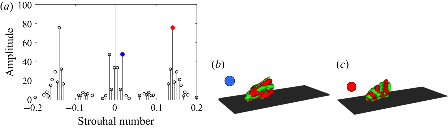
Figure 2. (a) Spectra of the dynamic modes for the non-reacting case selected by the sparsity-promoting algorithm. The dominant frequencies are highlighted by red and blue markers. Spatial modes at a frequency  $St = 0.016$ correspond to the blue marker (b) and at
  $St = 0.14$ correspond to the red marker (c). The red and green isocontours depict positive and negative wall-normal velocities, respectively. The dark surface represents the flat plate.
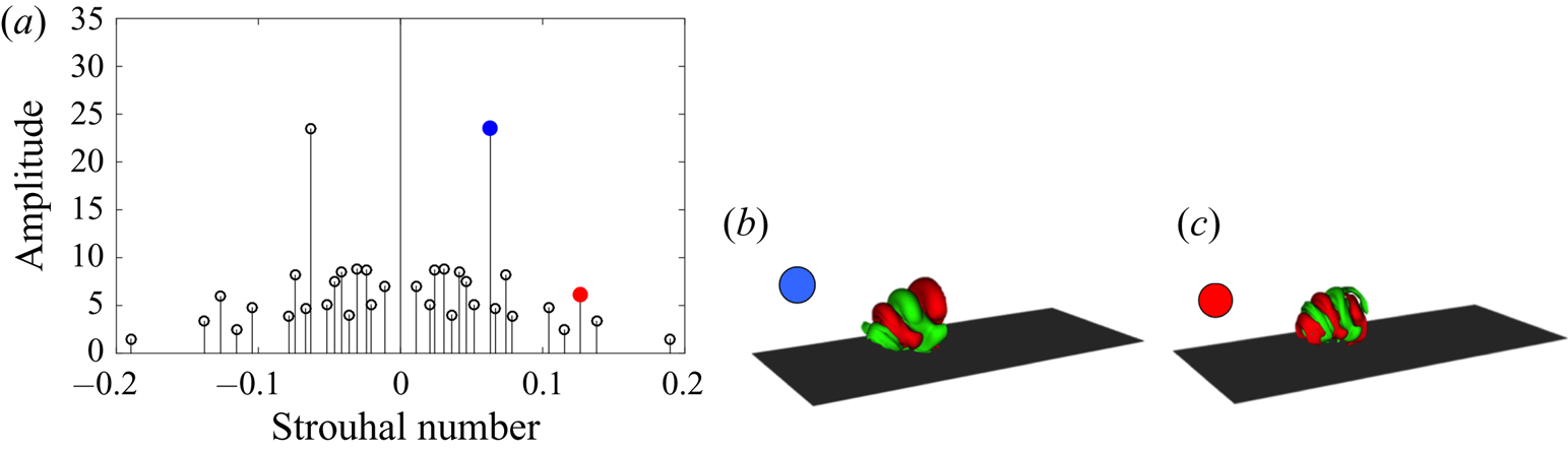
Figure 3. (a) Spectra of the dynamic modes for the reacting case selected by the sparsity-promoting algorithm. The dominant frequencies are highlighted by red and blue markers: spatial modes (b) at a frequency  $St = 0.06$ indicated by the blue marker and (c) at a frequency
  $St = 0.12$ indicated by the red marker. The red and green isocontours depict positive and negative wall-normal velocities, respectively. The dark surface represents the flat plate.
The lower-frequency structures are more dominant close to the wall, directly behind the separation bubble, while the faster structures have a dominant signature mostly in the shear layer of the jet. The prevailing modes in the reactive case, on the other hand, have different frequencies compared to the cold case. This latter case is driven by shear-layer instabilities, as both dominant modes correspond to a modulation of the shear layer, one with double the frequency of the other. The faster mode induces structures of a lower wavelength in the shear layer compared to the slower mode, suggesting a harmonic–subharmonic relation between them.
Comparing the frequency and the shape of the dominant modes extracted in both regimes suggests that the exothermic combustion process is accompanied by the strengthening of the subharmonic mode of the shear layer, leading to a pairing of vortical structures and the initiation of nonlinear behaviour along the upstream side of the jet, and yielding a transfer of energy from the fundamental to the subharmonic structure. This phenomenon, as reported also by Getsinger, Hendrickson & Karagozian (Reference Getsinger, Hendrickson and Karagozian2012), Strykowski & Niccum (Reference Strykowski and Niccum1991) and Megerian et al. (Reference Megerian, Davitian, Alves and Karagozian2007), is reminiscent of a convectively unstable jet. In contrast, in a globally unstable regime, a single frequency – evidence of limit-cycle behaviour – dominates, which is reflected as a single peak in the spectra for the case of a non-reactive jet. This is not surprising since, as demonstrated by Getsinger et al. (Reference Getsinger, Hendrickson and Karagozian2012), both the velocity and the density ratios of jet to crossflow affect the instability of the transverse jet. The exothermic characteristics of the combustion process alter the temperature inside the jet and consequently reduce the respective density of the flow, which can explain the shift to a lower Strouhal number in the dominant mode and even the change in the nature of the instability. Further and detailed instability analyses are, however, required to conclusively confirm these findings, and will be the subject of future research.
With pronounced differences in frequency and shape of the dominant structures depending on the absence or presence of reactive effects, we anticipate equally marked influences on the frequency response behaviour for either case. In order to quantify these influences, the governing equations are linearized about the base-flow solutions and the optimal energy gain is determined for selected driving frequencies, together with the associated input forcing and output response.
5.2. Base-flow solution
The base-flow solution  $\bar {{\boldsymbol {q}}}$ is taken as the steady-state solution of the nonlinear governing equations. We employ selective frequency damping (Åkervik et al. Reference Åkervik, Brandt, Henningson, Hœpffner and Marxen2006) to obtain the base flow by solving the following driven composite system of equations until convergence is achieved:
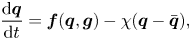 $$\begin{gather} \frac{\textrm{d} {{\boldsymbol{q}}}}{\textrm{d}t} = {{\boldsymbol{f}}}({{\boldsymbol{q}}},{{\boldsymbol{g}}}) - \chi({{\boldsymbol{q}}} - \bar{{{\boldsymbol{q}}}}), \end{gather}$$
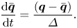 $$\begin{gather}\frac{\textrm{d}\bar{{{\boldsymbol{q}}}}}{\textrm{d}t} =\frac{({{\boldsymbol{q}}} - \bar{{{\boldsymbol{q}}}})}{\varDelta}. \end{gather}$$
 In the above expressions,  $\varDelta$ and
  $\chi$ are user-defined filter parameters that control the filter width and cut-off frequency. Figure 4 shows the base-flow solution calculated using selective frequency damping for both the reactive and non-reactive cases.
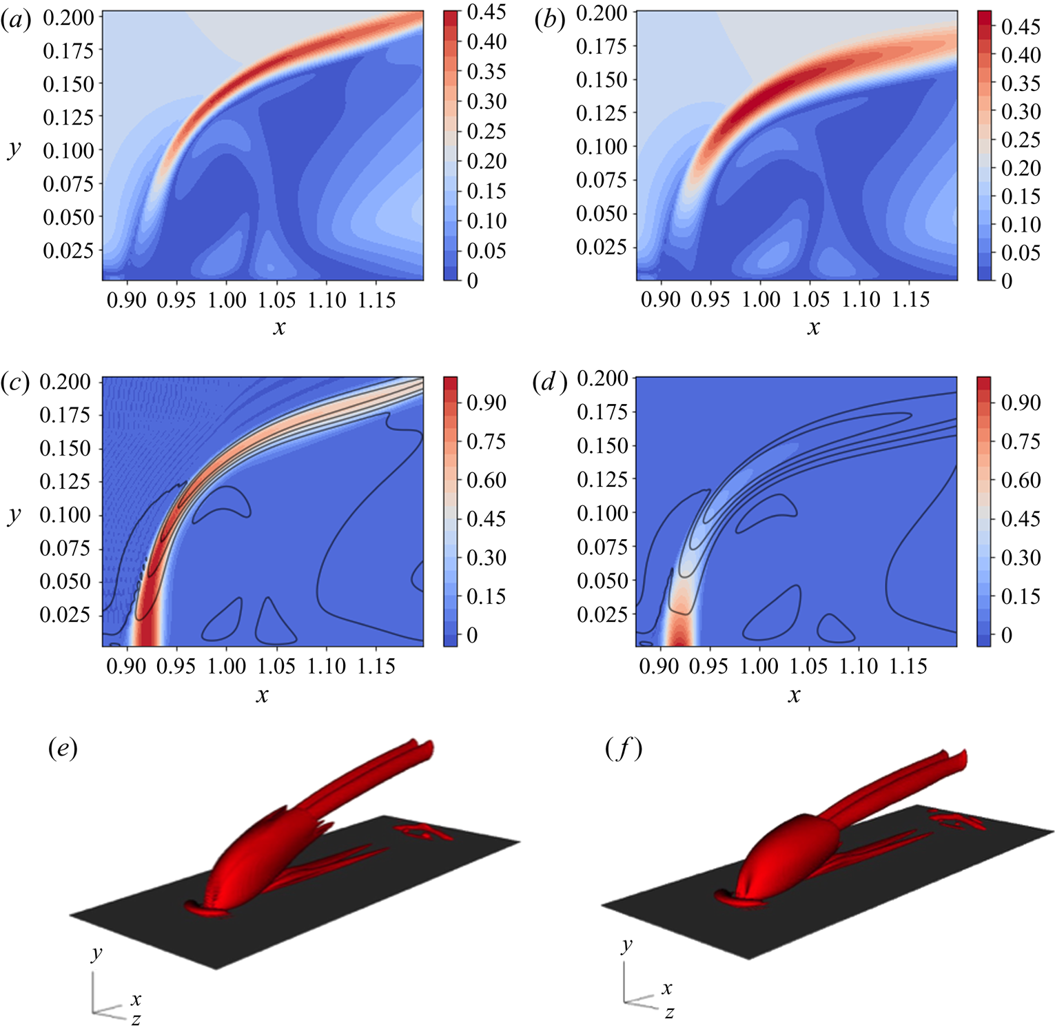
Figure 4. Base-flow solutions for both the reacting and non-reacting cases. Slices are presented at  $z = 0.15$, the midpoint of the computational domain. (a,b) Contours of velocity magnitude. (c,d) Contours of fuel mass fraction, solid contour lines representing the velocity magnitude. (e,f) Isosurfaces of the
  $Q$-criterion as an indicator of vortical flow structures. (a) Cold jet, velocity magnitude. (b) Hot jet, velocity magnitude. (c) Cold jet,
  $\rho Y_f$. (d) Hot jet,
  $\rho Y_f$. (e) Cold jet. (f) Hot jet.
Figures 4(a) and 4(b) compare the magnitude of the velocity vector for the reacting and non-reacting configurations. These figures suggest that the presence of reactions increases the thickness of the shear layer, impacting the size of the wake region behind the jet. This region appears to be wider in the streamwise direction of the reactive case compared with that in the non-reactive setting. On the other hand, due to the wider shear layer in the hot jet, the wake shrinks in the wall-normal direction. In figures 4(c) and 4(d), filled contours of the steady-state fuel mass fraction  $Y_f$ are compared for the non-reactive and reactive cases. The overlaid contour lines are the respective velocity magnitudes associated with the two cases. Due to the missing reactive effects in the former case, the fuel mass fraction acts, in effect, as a passive scalar with the flow providing the carrier fluid. This is evident in the shape of the base-flow solution, where the distribution of the scalar field closely follows the background flow. Figure 4(e) shows the vortical structure of the flow itself, visualized using isosurfaces of the
  $Q$-criterion (Hunt et al. Reference Hunt, Wray and Moin1988). The flow demonstrates the characteristic structure of a jet in crossflow, highlighted by a counter-rotating vortex pair. Considering the reactive jet, on the other hand, the signature of the fuel mass fraction is markedly different compared with the non-reactive case. Further downstream, however, as demonstrated by the vortical structures in figure 4(f), a counter-rotating vortex pair appears again, similar to the non-reactive case. Figure 4(d) also shows that
  $Y_f$ attains negligible values, before reaching the point where a counter-rotating vortex pair develops in the reactive case, confirming the previous observation that the flame extinguishes before the breakdown of the jet.
In order to compare the jet trajectory and penetration depth in both cases, contour lines of the velocity magnitude are superimposed in figure 5. This figure shows that the presence of reactions does not affect the near-field jet penetration. This finding agrees with previous results of jets with comparable jet-to-free-stream velocity ratios (see Wagner et al. Reference Wagner, Grib, Renfro and Cetegen2015). However, comparing the contour lines further downstream reveals a thicker shear layer in the reactive case. In addition, the size and shape of the recirculation zone are affected in the presence of reactions. It can thus be concluded that the exothermic process in the reactive case increases the temperature in the domain, which ultimately affects the viscosity level of the flow, as well as the generation and evolution of shear-layer vortices. This fact was also confirmed by instantaneous flow structures in the flow, shown in figure 1. The presence of reactions seems to slightly reduce the penetration depth of the jet in the wall-normal direction.
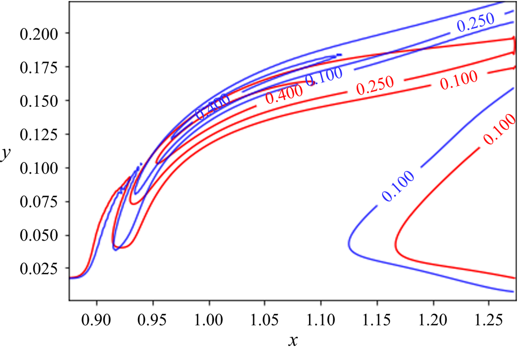
Figure 5. Contour lines of the velocity magnitude: blue, non-reacting case; red, reacting case.
In order to quantify the flame position and the region of highest heat release, the contour lines of the mean temperature field and the absolute value of the density gradient (as a numerical schlieren measure) are plotted in figure 6 for the reactive case. Contours of the density gradient reveal a thin region on the crossflow side of the jet with intense reactions, leading to the highest temperature values slightly downstream of the injection zone (demonstrated by a red contour line in the figure). In this configuration, the flame is significantly stronger on the crossflow side, leading to a flame distribution similar to that of Lyra et al. (Reference Lyra, Wilde, Kolla, Seitzman, Lieuwen and Chen2015), where the jet-to-crossflow momentum ratio is similar to the case considered here. The contours of the temperature and density gradient suggest an anchored flame on the crossflow side. The heat release is concentrated in the region where shear-layer vortices appear, impacting the unsteady development and evolution of these vortices as demonstrated by figure 1 and also reported for other studies (Nair et al. Reference Nair, Wilde, Emerson and Lieuwen2019b; Pinchak et al. Reference Pinchak, Shaw and Gutmark2019).
Figure 6. Steady-state solution of the reactive jet in crossflow at  $z = 0.15$. (a) Contours of the fuel mass fraction
  $\rho Y_f$ and contour lines of the temperature profile: red, 90 % of the maximum temperature. (b) Contours of the fuel mass fraction
  $\rho Y_f$ and density dilatation
  $\lVert \boldsymbol {\nabla } \rho \rVert$.
As demonstrated by Füri et al. (Reference Füri, Papas, Raïs and Monkewitz2002), the location of the flame with respect to the jet centreline can have a large impact on the development and frequency of the Kelvin–Helmholtz instabilities in the shear layer of the jet. In this case, the location of maximum temperature coincides with the jet centreline, and as demonstrated by Füri et al. (Reference Füri, Papas, Raïs and Monkewitz2002) this could bring about a stabilizing effect on the growth rate of unstable modes in the linear limit. This behaviour could explain differences in the flow structure during the initial development stage of the jet, as shown in figure 1. In addition, as demonstrated by Yule et al. (Reference Yule, Chigier, Ralph, Boulderstone and Ventura1981), for the case of a round jet, the reactive configuration can contain combustion/buoyancy-driven instabilities – in contrast to the cold jet, which is dominated by Kelvin–Helmholtz instabilities. The change in the source of instabilities was shown to also affect the resulting vortical structures in the jet. The hot jet was shown to have a longer potential core and undergo a slower transition to turbulence. Hence, the combination of flame position with respect to the shear layer and different instability mechanisms can be thought responsible for the change of flow structures in the two configurations.
5.3. Response to harmonic forcing
Low-level sinusoidal excitation has been used in jet-in-crossflow configurations to examine the growth of instabilities downstream, where time-periodic, spatially growing instabilities along the shear layer hint at a convectively unstable set-up, whereas instabilities that grow in time from their initiation point may suggest a global or absolutely unstable behaviour (see Huerre & Monkewitz Reference Huerre and Monkewitz1990; Megerian et al. Reference Megerian, Davitian, Alves and Karagozian2007). Forcing in this present study, however, is used within a different context. Adjoint-based analysis is utilized to extract optimal frequency and response eigenvectors resulting in maximum energy growth for a given time horizon  $T$. In addition, the forcing function is not confined to the nozzle inlet. As a result, the manner by which the disturbances evolve in time are not analysed here; instead, for a given frequency, the shape of the optimal forcing function is extracted and compared, for the presence and absence of exothermic reactions. The aim here is to identify the impact of the optimal forcing on both the shape and position of the forcing functional at a given frequency, and to quantify the resulting response.
At this stage, using the base-flow solutions computed in the previous section, optimal response and forcing functions corresponding to a given frequency,  $St = 0.1$, are extracted using the adjoint-based algorithm and are compared for the reactive and non-reactive cases. Considering the frequency spectra extracted from the nonlinear flow in both cases (figures 2 and 3), this frequency falls between the frequencies of the dominant modes identified in the figures. Within the linearized framework, no-slip velocities are used as boundary conditions for the velocity perturbations at the wall, and adiabatic conditions are employed for the energy. The mass fraction perturbation is set to zero at the wall, and all perturbation quantities are assumed to be zero in the free stream.
Figure 7 shows the spatial distribution of the optimal forcing and response functions, in the non-reacting case, for a harmonic forcing at a frequency  $St = 0.1$. The solution is visualized by the wall-normal velocity and fuel mass fraction components of the state vector; forcing and response solutions for other components show similar behaviour. The contours are plotted for the conservative form of the forcing function, which allows direct comparison with the response solution in conservative form. The contours of the optimal response function show perturbation velocities on the lower branch of the jet shear layer. The mode appears to be symmetric across
  $z = 0.15$ (middle of the spanwise axis), confirmed by the contours of the response fuel mass fraction shown in figure 7(f). The forcing solution for the selected frequency appears to concentrate inside the shear layer, slightly lower than the response location, suggesting a globally unstable configuration. The optimal forcing and response are therefore linked to the shear-layer instability of the globally unstable jet. Megerian et al. (Reference Megerian, Davitian, Alves and Karagozian2007) found experimentally that, for a low jet inflow ratio
  $R < 3.5$, external excitation has only a minor impact on the flow response. This is in contrast to the significant effect of forcing for larger values of
  $R$, suggesting a transition from a globally unstable flow, where intrinsic self-sustained oscillations are present, to a convectively unstable flow that exhibits noise-amplifying behaviour (Huerre Reference Huerre2007; Bagheri et al. Reference Bagheri, Schlatter, Schmid and Henningson2009). As a consequence, the response of the jet to forcing is directly dependent on the nature of its instability. The jets considered in this analysis are in the globally unstable regime (
 $R=3$), and the optimal forcing/response functions represent self-sustained oscillations.
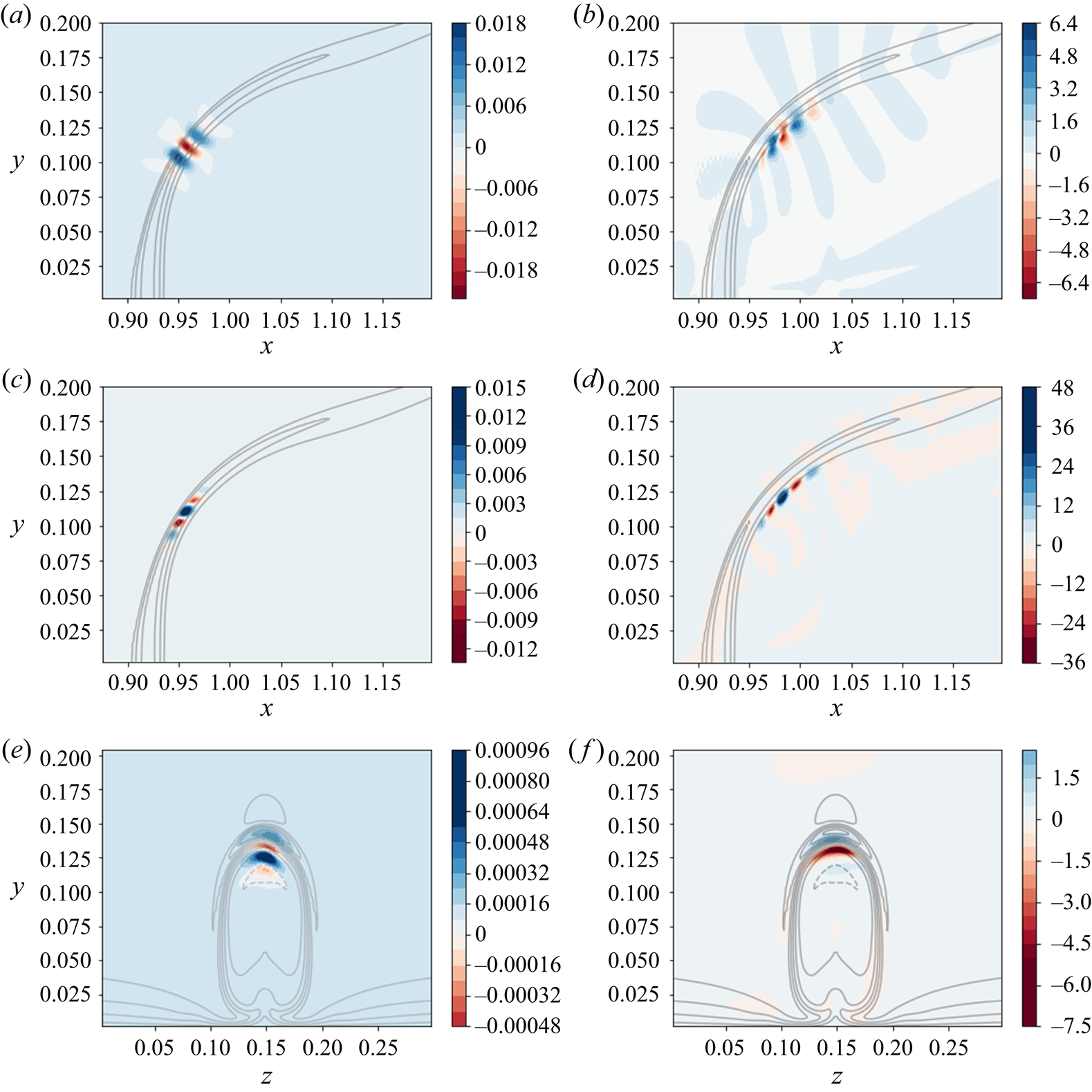
Figure 7. Forcing and response fields, non-reacting jet,  $St = 0.1$. (a,b) Contours of the wall-normal velocity component. (c–f) Contours of fuel mass fraction (passive scalar in this case). The contours are superimposed on contour lines of the steady-state passive scalar. (a) Wall-normal velocity forcing,
  $z = 0.15$. (b) Wall-normal velocity response,
  $z = 0.15$. (c) Fuel mass fraction forcing,
  $z = 0.15$. (d) Fuel mass fraction response,
  $z = 0.15$. (e) Fuel mass fraction forcing,
  $x = 1$. (f) Fuel mass fraction response,
  $x = 1$.
The shape and the location of forcing and response solutions of the fuel mass fraction, in this non-reacting case, are similar to those of the hydrodynamic variables. This behaviour is expected since the fuel mass fraction can be considered as a passive scalar in the absence of reactions. Owing to the direct effect of reactive terms on the steady-state solutions, it seems reasonable to expected a significant influence on the spatial distribution of the forcing and response functions in the presence of chemical reactions.
Figure 8 shows the spatial distribution of the optimal forcing and the corresponding response functions, in the reactive case, for a harmonic forcing at a frequency  $St = 0.1$. The lack of exact symmetry in some of the figures could be remedied with more iterations of the direct-adjoint algorithm. However, due to the high computational cost of this exercise, once the objective functional is adequately converged, the iterations are terminated. Similar to the non-reactive case, when considering the response solution, the perturbation velocity appears on the lower branch of the shear layer, shown in figure 8(b). Variations in the fuel mass fraction are negligible is this region, since most of the fuel has already been consumed, as shown in figure 8(d). As a result, the perturbation in the fuel mass fraction appears downstream of the region identified by the steady-state flame solution. When comparing the shape of the instability in figures 7(b) and 8(b), the response in the reactive case seems to have a larger wavelength, along the base-flow solution, than that in the non-reactive case. The forcing function, on the other hand, has an entirely different signature. When considering the velocity component of the forcing, it is active in the region including the largest variation in the fuel mass fraction. However, the forcing amplitude is higher on the edges, with the largest amplitude on the lower branch of the jet shear layer. While the forcing functions of the velocity components include perturbations inside the shear layer as well as in the flame region, the perturbations are present only in the flame region as far as the mass fraction and density (not shown here) are concerned. Combining the effects of forcing in the velocity (figure 8a) and mass fraction (figure 8c) components on the base-flow solution, we observe a pronounced wrinkling at the tip of the fuel mass fraction contours, as shown in figure 8(a), which in turn induces a flame instability. Similar behaviour was also observed and analysed for a thermo-acoustically forced
  ${\boldsymbol{\mathsf{M}}}$-flame by Blanchard et al. (Reference Blanchard, Schuller, Sipp and Schmid2015). Comparing the results of figures 7 and 8 shows that, while in the non-reactive case forcing inside the shear layer leads to highest growth in the energy of the system, suggesting a shear-layer instability, in the reactive case, forcing functions modulating the flame distribution yield the highest energy gain. In addition, the reacting cases show some overlap between the spatial locations of the forcing and the response which would suggest that these cases do not exhibit globally unstable behaviour, at least not to the same degree as the inert cases.

Figure 8. Forcing and response fields, reacting jet,  $St = 0.1$. (a,b) Contours of the wall-normal velocity component. (c–f) Contours of fuel mass fraction (passive scalar in this case). The contours are superimposed on contour lines of the steady-state passive scalar. (a) Wall-normal velocity forcing,
  $z = 0.15$. (b) Wall-normal velocity response,
  $z = 0.15$. (c) Fuel mass fraction forcing,
  $z = 0.15$. (d) Fuel mass fraction response,
  $z = 0.15$. (e) Fuel mass fraction forcing,
  $x = 1.0$. (f) Fuel mass fraction response,
  $x = 1.0$.
Varying the forcing frequency does not appreciably affect the shape of the response and forcing functions; however, the optimal energy gain will differ. In the following section, we investigate the impact of the forcing frequency on the total energy gain of the system.
5.4. Frequency response of a (non-)reactive jet
In this section, the frequency responses of the reactive and non-reactive jets in crossflow, for a range of frequencies corresponding to  $0.05 \leqslant St \leqslant 0.14$, are extracted and analysed. The range of frequencies has been selected based on the spectra presented in figures 2 and 3, taken from the analysis of the nonlinear flow. Since the lowest frequency of the inert case (
 $St = 0.016$) is related to wall vortices, it has not been included in the analysis. Instead, the forcing frequency is varied within the interval
  $0.05 \leqslant St \leqslant 0.14$, which includes both dominant frequencies identified in the reactive regime, as well as the highest frequency of the non-reactive case. The time horizon (
 $T_f$ in (3.2)) is set to half the period of the case with
  $St = 0.1$ for all frequencies. A careful analysis showed that changing the time period does not noticeably affect the shape of the modes, or the trend of the frequency response plots presented in this section. The gain curves, illustrating the frequency response for each regime, are fitted by cubic Hermite interpolation, using the gain values together with the values of the local frequency gradient extracted using the adjoint-based algorithm described in § 3.
Figure 9(a) shows a nearly linear increase in the energy gain of the inert system as the frequency increases. This increase is also confirmed by the extracted gradients using the expression presented in (3.6). All frequency gradients extracted for  $0.08 \leqslant St \leqslant 0.14$ have approximately the same value. This quasi-linear increase is due to the fixed time horizon for each frequency. Since the identified mode is related to shear-layer instabilities (shown in figure 7) for all considered frequencies, augmenting the frequency increases the energy gain by accounting for a larger portion of the disturbance period.
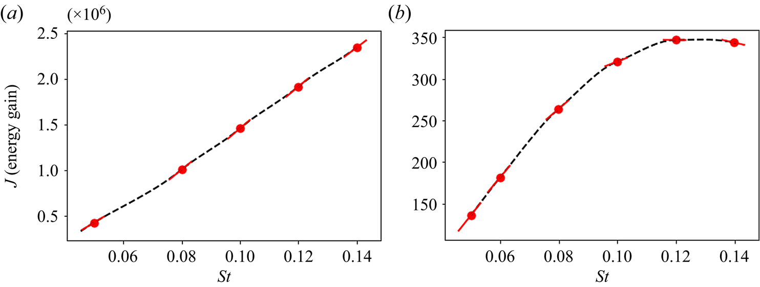
Figure 9. Frequency response of the two configurations: (a) non-reactive jet; (b) reactive jet. Red circles, locations where  $J$ and
  $\textrm {d}J/\textrm {d}\omega$ are extracted using the adjoint-based algorithm; solid red line, local gradient; black dashed line, cubic Hermite interpolation.
On the other hand, figure 9(b) shows a distinctly different behaviour in the frequency response in the presence of reaction. While the energy gain increases monotonically, similar to the inert case, it reaches a maximum at  $St = 0.12$ after which it starts to decrease. This is also confirmed by the extracted frequency gradients, which decrease as the forcing frequency grows, until they finally change sign in the vicinity of
  $St = 0.12$. Hence, within the range of frequencies considered here, an optimal forcing frequency is identified for the reactive configuration. This optimal frequency is similar to the harmonic frequency identified while analysing the nonlinear spectra of the jet, shown in figure 3.
Comparing the frequency response for both jets in crossflow shows the substantial impact that reactions have on the system's response. Although both jets are globally unstable, the presence of reactions alters the shape of the optimal forcing and response modes, as well as the energy gain of the system.
6. Summary and conclusions
Simulations of reactive and non-reactive jets in crossflow, with a jet-to-crossflow velocity ratio of three ( $R = 3$), have been performed using a compressible direct numerical simulation framework. The combustion has been modelled by lean reactions, resulting in an additional transport equation for the fuel mass fraction. Both the crossflow and the flow at the inlet of the jet have been assumed laminar. Due to the interaction of the jet with the transverse flow, instabilities develop along the curved jet shear layer causing roll up and eventual breakdown into turbulence.
Performing a dynamic mode decomposition on the data gathered from the nonlinear solutions of both configurations and comparing the resulting spectra show a substantial impact of reactive effects on the dominant frequencies in the flow. While the extracted frequencies in the inert case compare well with simulations of Bagheri et al. (Reference Bagheri, Schlatter, Schmid and Henningson2009), the reactive jet in crossflow shows substantially lower frequencies corresponding to the shear-layer instability. The flow structures also differ from those of the non-reactive jet in crossflow, as the reactive jet penetrates the crossflow noticeably less in the vertical direction.
The steady-state solution of both configurations has been determined using selective frequency damping Åkervik et al. (Reference Åkervik, Hœpffner, Ehrenstein and Henningson2007). Optimal forcing and response structures have then been identified using an adjoint-based optimization methodology coupled to the solver. This framework is particularly efficient, since the linearized operators are computed simply by using a local differentiation technique, without explicitly forming the resulting matrices for both forward and adjoint operators. In the inert case, the forcing and response functions are concentrated inside the shear layer of the jet, as expected from a globally unstable flow. However, in the reactive jet, the forcing functions show support inside the flame, and the forcing fuel mass fraction together with the velocity components create structures that induce wrinkling near the tip of the flame, suggesting a link to a flame instability. Therefore, the presence of reactions visibly alters the modal shapes extracted from this configuration. In addition, studying the jet response to various forcing frequencies in both regimes shows a different behaviour within the range of considered frequencies. In contrast to the non-reactive case, an optimal forcing frequency is identified in the reactive setting.
While these results establish a definitive impact of chemical reactions on the optimal forcing and response of the jet, there still remain a few open questions. As mentioned earlier, the considered jet-to-crossflow velocity ratio results in a globally unstable jet. Higher ratios will, however, result in a convectively unstable flow, altering its receptivity to forcing and motivating a similar analysis in this parameter regime. In addition, turbulent jet-in-crossflow configurations commonly operate in higher-Damköhler-number  $(Da)$ regimes. Hence, the effect of
  $Da$ should be analysed by considering more sophisticated kinetic models. Investigations in these directions will be the subject of future research efforts.
Acknowledgements
The authors would like to thank Mr P. Sashittal for providing the data for the nonlinear and base-flow solutions. We would also like to thank one of the reviewers, whose input strengthened the scientific content of this work.
Funding
This research received no specific grant from any funding agency, commercial or not-for-profit sectors.
Declaration of interests
The authors report no conflict of interest.


 Open access