Large-Scale Landslide Susceptibility Mapping Using an Integrated Machine Learning Model: A Case Study in the Lvliang Mountains of China

Introduction

Landslides are one of the most dangerous mass movements in mountainous areas, resulting in substantial loss of life and damage of property on a yearly basis (Petley, 2012; Chen et al., 2017a; Guo et al., 2018). Many potential landslides also bring severe challenges to the risk management of geological disasters (Klimešl et al., 2017). In addition, the demand for land is increasing with the acceleration of urban construction. However, the high risks caused by the uncertainty of landslide disaster seriously restrict land use planning in landslide-prone areas (Fell et al., 2008). Consequently, proper strategies or measures for landslide risk mitigation are increasingly attracting the attention of the academia, especially at this stage (Van Westen et al., 2008).

Landslide susceptibility evaluation is considered the first step to understand a basic concept of risk assessment and its influences (Van Westen et al., 2003; Fell et al., 2008). Its outputs called landslide susceptibility maps allow users to know the areas where landslides can easily initiate and propagate (Guzzetti et al., 1999; Guzzetti et al., 2006). Based on the division of evaluation units and the selection of environmental factors within study areas, selecting a suitable model is of importance to obtain effective results (Ahmed, 2015). According to previous literature, landslide susceptibility models can generally be divided into four categories: heuristic models, deterministic models, statistical statistics, and machine learning models (Huang et al., 2017; Sezer et al., 2017; Broeckx et al., 2018; Reichenbach et al., 2018; Medina et al., 2021). Among these models, heuristic models can be considered as knowledge-based models which depend much on the experts’ opinions on the geomorphology and historical landslides; thus they are highly subjective (CastellanosAbella and Van Westen, 2008). Deterministic models are normally physically based, which need accurate geotechnical parameters over large areas (Bueechi et al., 2019). However, these parameters are usually related with large uncertainties, and the computational time of these models can be long (Crippa et al., 2016; Tofani et al., 2017). Hence, statistically based models and machine learning models are the most commonly used techniques during the past decade (Reichenbach et al., 2018). Meanwhile, some comparative studies have confirmed that these models normally have better performances than other types of models when dealing with the same study areas (Goetz et al., 2015; Aditian et al., 2018; Huang et al., 2020).

As is known to all, in the process of regional landslide susceptibility modelling, it is common to analyze the relationship between the historical landslides and environmental factors. Because landslides are inherently complex nonlinear processes, various factors are selected by researchers to capture more information on the development of landslides. Compared with statistically based models, machine learning models normally have the advantages of higher accuracy in calculating the nonlinear relationship (Achour and Pourghasemi, 2020). They do not require the environmental factors to be normally distributed and are also suitable for large areas. Accordingly, at least dozens of machine learning models have been reported until now, such as the back propagation (BP) network, tree-based models, multilayer perceptron (MLP), support vector machine (SVM), extreme learning machine (ELM), clustering, random forest (RF), Bayesian network (BN), XGBoost models, and so on (Ermini et al., 2005; Catani et al., 2013; Bui et al., 2016; Chen et al., 2017b; Huang et al., 2017; Pham et al., 2017; Chen and Li, 2020; Can et al., 2021).

Although various machine learning models are available now, every single model has its own advantages and disadvantages. Hence, it is still important to compare the performances among different models for specific landslide susceptibility practices. Moreover, the integration of models provides another option, which may improve the model accuracy by combining the advantages of different models. Hence, it is highly encouraged to produce “optimal” susceptibility models by combining multiple models (Reichenbach et al., 2018). However, it is of difficulties to determine how to best integrate multiple forecasts to obtain better results Rossi et al. (2010), and limited attempts have been made on this issue, especially regarding the integration of machine learning models (Sevgen et al., 2019; Kocaman et al., 2020).

Hence, the present study aims at testing if the integrated machine learning model can obtain better results than individual models. In order to make more readers clear to the modelling process, three models that are commonly used were selected as the basic models, namely, the BP, SVM, and RF models. Our objective mainly focused on the way of integrating these models and the production of a better model. Specifically, the purposes of this study include (a) using the frequency ratio method to analyze the nonlinear relationship between the landslide inventory and causal factors in a region located at Lvliang mountains of China, (b) integrating different machine learning models where their connecting weights to susceptibility results were optimized by the GWO algorithm, and (c) applying different models to generate the regional landslide susceptibility maps and comparing their performances.

Study Area

The study area (35°43′–38°43′ N, 110°22′–112°19′ E) is located in southwestern Shanxi Province and covers an area of approximately 21,140 km². It includes four counties: Shilou, Yonghe, Ji, and Daning (Figure 1). Geomorphologically, the area belongs to the Lvliang mountains of Central China and is surrounded by moderately high and low mountains. Elevation varies from 399 m to 2,034 m above sea level and increases from west to east. Based on geological data, the area is characterized by Cambrian to Jurassic sedimentary rocks and quaternary deposits. Sandstone, mudstone, sandy mudstone, and quaternary loess strata outcrop extensively (Tang et al., 2020). The area has a warm temperate continental monsoon climate with long cold winters and hot summers. Data from the local meteorological station shows that the average annual temperature and precipitation are 7°C and 514.9 mm, respectively. More than 60% of the total annual precipitation falls in summer (June–September). There are many settlements in the territory, so it is highly populated in some parts of the area. During the urbanization, the original topography has been modified by engineering activities (e.g., the construction of transportation lines), which subsequently caused the slope deformation and instability.

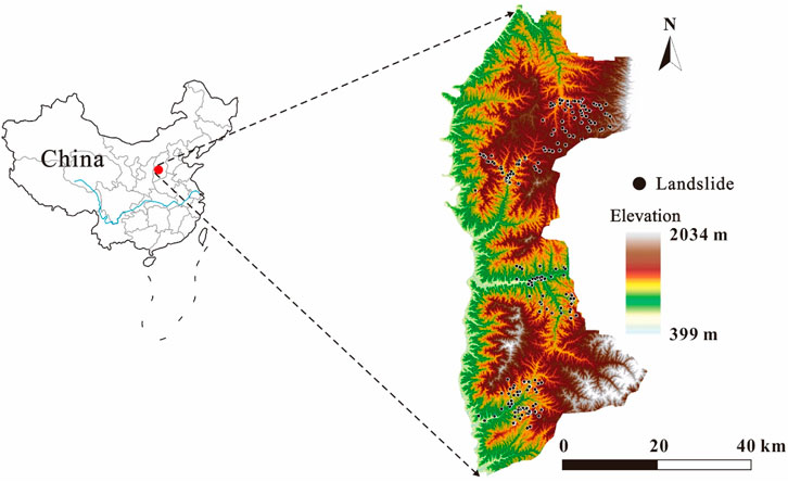
FIGURE 1. Landslide spatial distribution map.

Materials and Methods

Data Sources

The main software used in this study was ArcGIS 10.2. The first step was the data collection, which is the basis of landslide susceptibility analysis. The main data sources included the following (Table 1): (1) The digital elevation model (DEM) with a resolution of 25 m was provided by the China Geological Survey (Xi’an Center), which was subsequently used to generate other influencing factors, such as slope, aspect, and so on. (2) The geological map was used to extract information of soil and lithology. (3) The distribution map of landslides in the region was used to determine the landslide locations. (4) Remote sensing images obtained from Google Earth (https://www.google.com/earth/) were used to verify and calibrate the landslide location. (5) Landslide field survey reports were used to update the specific information of landslides (e.g., the date of occurrence, volume, material composition, and thickness of weak interlayer). (6) According to the monitoring data provided by the geological disaster management department, the local rainfall situation for many years was determined.

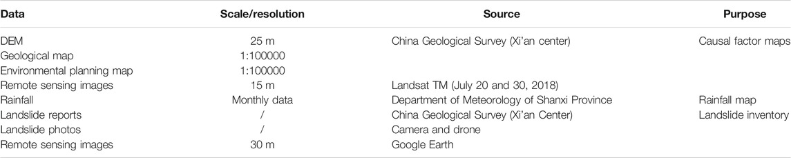
TABLE 1. Detailed data and their sources used in this study.

Landslide Inventory Mapping

Landslide inventory map can reveal the spatial distribution of landslides and is a necessary means to analyze the relationship between the landslide points and inducing factors (Tian et al., 2019). The study area is a landslide-prone area, which suffered many landslide hazards with various scales in history (Wang et al., 2019; Tang et al., 2020). To obtain the updated information of landslides in the area, several filed surveys were conducted during 2016 and 2018. The location of each landslide expressed by the X and Y coordinates of the central point was recorded. Meanwhile, the landslide reports provide basic information on each landslide, including volume, area, materials, and occurrence time. During the next stage, these landslides were digitized into the GIS environment, with the characteristics saved in the attribute tables. After this, the remote sensing images from Google Earth were used to crosscheck the location of landslides. The method used was mainly the visual interpretation. The landslides were confirmed if evident deformation or scarps were observed.

Finally, there are total 466 landslides in the area revealed by the landslide inventory map, among which 234 are loess landslides and 232 are rockfalls (Tang et al., 2020). Given that the mechanisms of the two types of landslides are totally different, this study only deals with the issue associated with loess landslides. According to the landslide classification criteria (Cruden et al., 1996; Hungr et al., 2014), most loess landslides in the area are large slope failures and composite soil slide–debris flows. A small number of landslides are earth slides.

From the number perspective, Jixian County has the largest number of loess landslides (72) while the number of landslides in Yonghe County is relatively small (49). Regarding the triggering factors of the landslides, there are two main reasons that make the study area prone to landslides. One is the unique structural properties and water sensitivity of loess which distributes extensively in the Lvliang mountains (Derbyshire, 2001). Geohazards are easily induced under heavy rainfall due to such properties (Wang et al., 2014; Zhuang and Peng, 2014). The other one is human engineering activities. The slope instability occurs when the slope angle is relatively large and the external disturbance also exists (Chen et al., 2019). In addition, landslides appear to have clustered in moderate elevations. This fits with the results in some other study areas (Catani et al., 2013; Medina et al., 2021). On one side, topography in low elevations is generally flat. On the other side, there are very few people and human activities in high mountains; thus landslide is hardly to happen or be identified.

Selection of Evaluation Units

A key problem in the development of landslide susceptibility mapping is how to divide “evaluation units.” Common division methods mainly include (Ba et al., 2018) grid, natural slope, subbasin, homogeneous conditions, and administrative division units. Among them, grid and slope units are the most frequently used. Current slope division methods still have some defects in practical applications, such as low operability, being very dependent on manual correction, etc. (Chen et al., 2019). On the contrary, the grid unit method has the advantages of convenient rapid subdivision, regular shape, and so on. Hence, the grid was selected as the evaluation unit in this study.

Proposed Integrated Model

In the previous studies, individual BP, SVM, and RF models have shown good performances in the analysis of landslide susceptibility (Ermini et al., 2005; Catani et al., 2013; Bui et al., 2016; Chen et al., 2017b). However, it is evident that various machine learning models have their own advantages and disadvantages when they are designed. Hence, we are curious if the accuracy can be improved when different models are integrated into one model. Hence, the BP-SVM-RF model was proposed in this study to test this point. Considering the individual BP, SVM, and RF models have been widely used, we only introduced the principles on the integration of them. The details of these three models have been described and explained in literature (Ermini et al., 2005; Catani et al., 2013; Bui et al., 2016; Chen et al., 2017b).

Figure 2 illustrates the framework of the integrated method. The integrated model takes BP, SVM, and RF as benchmark models and trains them to solve the same problem (landslide susceptibility evaluation). Furthermore, three weighting factors ($w_1$, $w_2$, and $w_3$) are used to combine the output results of the three models to obtain better results. Assuming that the output results of BP, SVM, and RF are ${\widehat{y}}_{BP}$, ${\widehat{y}}_{SVM}$, and ${\widehat{y}}_{RF}$, respectively, the output of the designed integrated model is (represented by ${\widehat{y}}_{Integrated}$) as follows:

where$w_1$, $w_2$, and$w_3$are real numbers between 0 and 1.

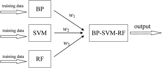
FIGURE 2. Framework of integrated model.

To determine these three weighting factors ($w_1$, $w_2$, and $w_3$), the following cost function (objective function) is constructed with the root mean square error:

where $y_{actual}$ is the result of susceptibility evaluation (0 or 1), and N is the number of training samples. It should be noted that the $y_{actual}$ is not a calculated value but an observed value. For a specific cell in the training samples, this value is 1 if a landslide point is located here. If this is a nonlandslide point, the value of $y_{actual}$ is 0.

To minimize the cost function, a heuristic optimization algorithm is used to obtain the numerical solutions of w₁, w₂, and w₃. Among the heuristic optimization algorithms, the gray wolf optimizer (GWO) is an algorithm with superior performance, which can avoid the premature convergence of the algorithm (Mirjalili et al., 2013). It has been successfully applied in the academe practices (Mirjalili, 2015; Guo et al., 2020). Therefore, the GWO algorithm was used in this study to obtain the optimal solution that minimizes the cost function. The $w_1$, $w_2$, and$w_3$calculation based on the GWO algorithm prognostics consists of six steps:

Step 1: The GWO algorithm parameters, including gray wolf population, maximum number of iterations, and the position $Q_k=[Q_{\alpha }(t+1),Q_{\beta }(t+1),Q_{\delta }(t+1)]$of each gray wolf are initialized. $t=1$ is set.

Step 2: Three dominant wolves in the population are identified and named as $\alpha$, $\beta$, and $\delta$in turn. These three wolves will lead the population to encircle, hunt, and attack prey (target solution).

Step 3: The convergence factor is calculated, and the coefficient vector is updated:

where $r_1$and $r_2$are random vectors between 0 and 1.

Step 4: The locations of these three best gray wolves are updated:

Step 5: The individual position in population is updated:

Step 6: If the iteration of the algorithm is terminated, the optimal individual position in the population is output; otherwise, return to Step 2.

For the integrated model, our goal was to find the best-fit values for the three weights (w₁, w₂, and w₃), whereas the results of the GWO were the optimized location of three dominant wolves (Q_α, Q_β, and Q_δ). Hence, the outputs obtained from the GWO were the results of the three weights. Users only need to input three initial values for the weights which should be between 0 and 1. Last, it should be mentioned that the present method is to integrate different models so it is a separated process from the landslide susceptibility map. In other words, other models can also be integrated by using this process.

Landslide Causal Factors

In the models for landslide susceptibility zonation, the environmental factors that affect the development of landslides are the input parameters of the model. Therefore, selecting the causal factors is an important step in this process. In the existing literature on this topic, several factors have been widely accepted (e.g., slope and lithology), while some other factors (e.g., curvature, soil map, and topographic wetness index (TWI)) remain controversial (Segoni et al., 2012; Arabameri et al., 2020). However, the performance of landslide susceptibility models is normally data-dependent, which means not only causal factors but also other data (e.g., the data availability and resolution) can affect the results (Catani et al., 2013). Hence, a causal factor may have different effects on landslides in different test occasions as the geological background of every area is unique (Tang et al., 2020). In view of this, several controversial but common factors in the literature were still selected in this paper.

To begin with, 15 causal factors, which have been widely used, including altitude, slope angle, aspect, plane curvature, curve curvature, relief degree, lithology, slope structure, land use, vegetation coverage, soil erosion intensity, TWI, distance from river, distance from highway, and rainfall, were identified as the initial database. Every factor was related with one aspect of landslide occurrence, including geomorphic characteristics, geological environment, environmental background, hydrological factors, and triggering factors. Several other factors are not selected due to the following reasons: Firstly, they do not occur frequently in the study area (such as earthquakes and freeze–thaw). Secondly, they have not been widely used before (such as soil properties and solar radiation). In the next stage, expert opinions on these factors were solicited. Five factors were suggested to be removed from the database, namely, the distance from the water system, distance from the highway, relief degree, slope structure, and topographic wetness index for the following reasons: 1) A certain overlap exists between the range of topography relief degree and curvature. 2) The TWI has a great relationship with debris flows, but almost no debris flow is observed in the study area. 3) The direction of the stratum is the same as that of the slope in this area, which has a negligible relationship with slope structure. 4) The distance from the water system and highways are related to rainfall accumulation because rivers and roads normally have low elevations. Hence, these two factors were also deleted to make the rainfall an independent variable in the factor system. Subsequently, the results of the correlation analysis among each factor supported the expert’s opinion: The five removed factors really had a correlation coefficient of more than 0.5 with a certain one or several factors, thus indicating they were not independent variables. Hence, it is reasonable to remove them from the influencing factors system, which can improve the conditional independence of the model (Pereira et al., 2012).

Finally, the evaluation factor system was established containing 10 factors. It should be stated that all the models used these 10 factors to generate landslide susceptibility maps. This is mainly because the main objective of this study is to compare the accuracy between individual and integrated model. Hence, besides the model used, the other settings should keep constant, specially the conditioning factors. These factors included both discrete and continuous variables, such that the continuous factors should be separated into several categories in a fixed manner when using the proposed model. However, no uniform standard exists for the number of intervals. Generally, 4–12 intervals are considered as suitable, because too many intervals will increase the model complexity while too few intervals cannot reflect enough information of factors (Chen et al., 2017c; Huang et al., 2020). Finally, all continuous factors were divided into 4–9 intervals in this study. Frequency ratio (FR) was used to measure the landslide density in each interval of the factor. This method can be expressed as the ratio of the percentage of landslide contained in each factor category to the percentage of area occupied by the corresponding category (Aditian et al., 2018). The results of FR analysis are showed in Table 2. The detailed preparations of each factor and reclassification are described as follows.

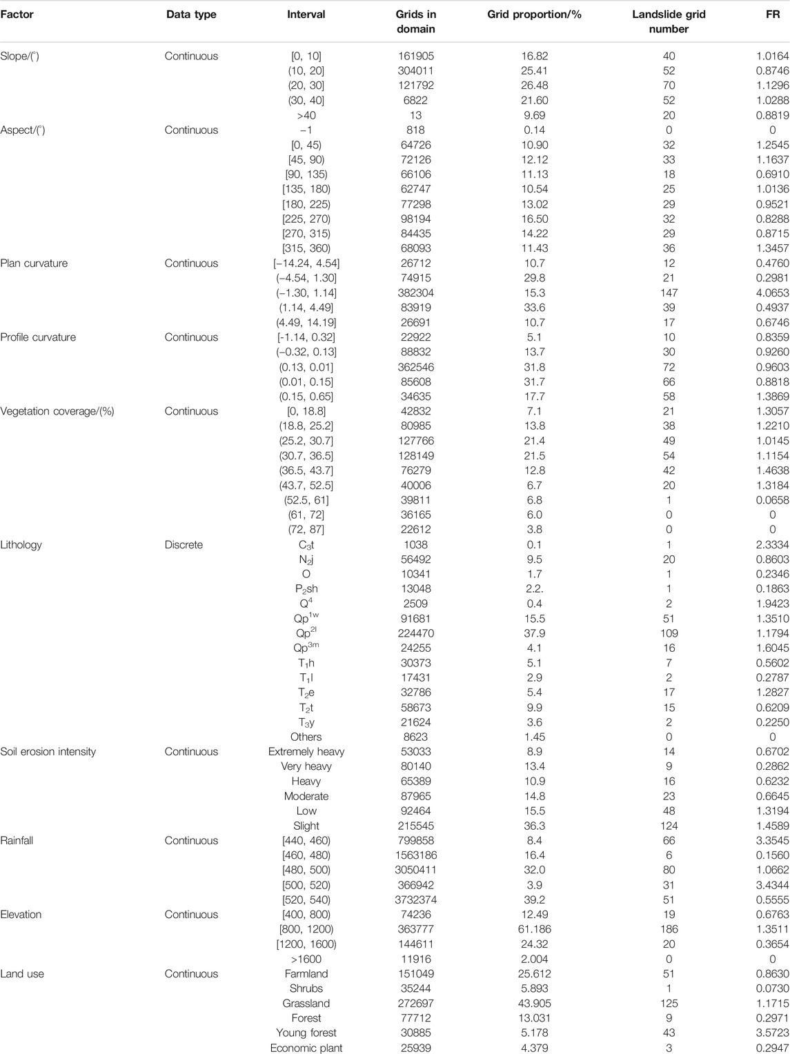
TABLE 2. Frequency ratios of index factors.

Elevation (Figure 3A): Occurrence of landslides is closely related to the elevation as the environmental conditions of slopes, such as land coverage, climate, and human activities, vary with the elevation (Guo et al., 2019). The DEM showed that the altitude of the area ranged from 399 to 2,056 m asl. It was divided into four grades with 400 m intervals. Table 1 shows that the FR of the elevation in the range of 800–1,200 m is greater than 1, which indicates that this elevation interval has an important effect on landslide occurrence.

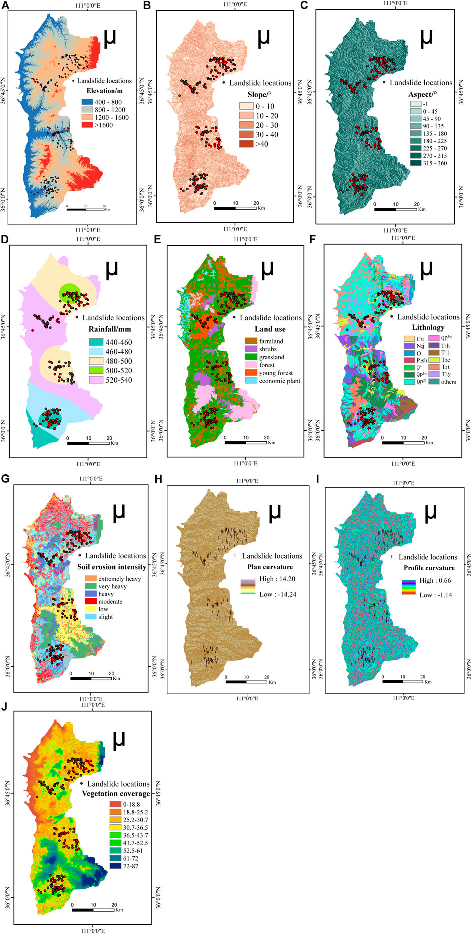
FIGURE 3. Causal factors used in landslide susceptibility modelling. The red dots represent landslide points in the study area: (A) elevation, (B) slope, (C) aspect, (D) rainfall, (E) land use, (F) lithology, (G) soil erosion intensity, (H) plan curvature, (I) profile curvature, and (J) vegetation coverage.

Slope (Figure 3B): Slope is an important factor to mirror the terrain, and it macroscopically reflects the fluctuation of the terrain. The higher the slope is, the more concentrated the shear stress is, and the more likely the landslides will occur. Moreover, the slope affects the erosion and erosion of surface runoff, vegetation coverage, and the supply and discharge of groundwater on the slope (Tang et al., 2020). The slope map was extracted from DEM using the GIS tool. The slope values in the region ranged from 0° to 60° and 10° intervals were used to divide them into five categories. The FR in the range of 10°–20° and 30°–40° were the largest, indicating that landslides mainly occur on moderate slopes.

Aspect (Figure 3C): This factor has an impact on the conditions on slopes, such as sunshine duration and solar radiation intensity, which can affect vegetation development, evaporation, weathering, and slope erosion (Youssef et al., 2015). At the same time, pore water pressure changes with temperature, such that slope stability and slope direction are also correlated. The map was also generated from DEM and was automatically recognized into nine main directions (interval 45°) in the GIS, where −1 was flat ground. The number of landslides and FR values in each class showed that the landslide density was higher when slopes were facing the north (0–90°, 270–360°).

Rainfall (Figure 3D): The main reasons to consider rainfall as a conditioning factor for landslide susceptibility in this study include the following: (i) The rainfall distribution in the study area has a spatial variability. (ii) This factor also has been considered in some previous studies (Catani et al., 2013). The influence of rainfall on slope stability is mainly manifested in three aspects (Guo et al., 2020; Medina et al., 2021): The first is the softening of rock and soil by rainfall infiltration, which weakens them. The second is the hydrostatic pressure and hydrodynamic pressure formed by rainfall infiltration, and its floating force constitutes an unfavorable factor for slope stability. The third is the erosion and destruction of slopes due to the erosion of runoff caused by rainfall. In this study, the daily rainfall of multiple rainfall monitoring stations was obtained first, which was used to generate the whole rainfall map by applying the Kriging interpolation tool in GIS. The map showed that the average annual rainfall in this area was between 440 and 540 mm, and it was divided into five categories at 20 mm intervals.

Land use (Figure 3E): Land use and its change can also trigger landslides (Shu et al., 2019). Various vegetation’s types show the difference in the degree of human disturbance and damage to the rock and soil; thus the probability of landslides is also different. Several land use types, such as forestry land, are conducive to slope consolidation and landslide reduction. Several land uses, such as cultivated land and residential land, can destabilize damage slopes. In this study, the land use map was generated from the Landsat TM image by using the object-oriented segmentation method. This step was completed in the recognition software, which segmented the image into different polygon objects automatically (Chen et al., 2019). Next, the attributes of on each land use type were captured and identified, mainly including geometrical and spectral features. To reclassify land use types, users need to (i) conduct field work to determine each land use type and corresponding features in RS images; (ii) select the training and testing samples from the segmented objects; (iii) reclassify the whole area into various land use types according to images features. The reclassification method used in recognition was the nearest neighbor method, and finally six types of land use maps were obtained: farmland, shrubs, grasslands, forests, young forests, and economic plants. The reason for distinguishing between forests and young forests is that forest coverage and density may change with age, leading to different landslide distributions. Economic plants were identified mainly because they may represent human activities with different intensities compared with other natural vegetation (Tang et al., 2020).

Lithology (Figure 3F): In this study, the stratigraphic lithological map was obtained from the regional geological map. The outcropping strata in the study area include Ordovician (o), Carboniferous (c), Permian (P), Triassic (T), Neogene (N), and Quaternary (Q) units. The Triassic and Quaternary strata cover most of the study area, such that they can be divided into several units according to age.

Soil erosion intensity (Figure 3G): Large amounts of soil resources have been eroded and destroyed, ravines have intensified, soil layers have become thinner, and large areas of land have been cut to pieces, which can easily cause geological disasters such as landslides and soil creep (Shrestha et al., 2004; Cuomo and Della Sala, 2015). In particular, the Loess Plateau has been suffering from loess landslides (Zhuang et al., 2018). In this study, the soil erosion intensity map was provided by the Shanxi Provincial Department of Surveying and Mapping, and six categories were classified.

Plane curvature (Figure 3H): It describes the characteristics of the terrain in the horizontal direction, which is equal to the change in the slope direction at a certain grid (Huang et al., 2017); thus, it can be obtained by deriving the slope direction in GIS.

Profile curvature (Figure 3I): It describes the complexity of the terrain, and it was also derived from the DEM, which was divided into five classes.

Vegetation coverage (VC) (Figure 3J): Vegetation can improve slope stability by strengthening soil and absorbing water. According to the field investigation, the area with less vegetation and low coverage in the Lvliang mountains has strong weathering erosion and serious soil erosion, which easily induce landslides. Thus, it is necessary to include the vegetation coverage map into the analysis. Two Landsat TM images were used to generate this map, namely, the images from July 20, 2018 (path 126, row 34), and July 30, 2018 (path 126, row 35), respectively. The multispectrum information in the images was used to calculate the vegetation coverage as follows (Chang et al., 2020):

where the P(NIR) and P(Red) are the spectral reflectance measured from the near infrared and visible red bands in the Landsat TM data.

Data Preprocessing

Machine learning models require sample data to conduct the landslide susceptibility modelling, because it is not possible to include the dataset of the entire area into the training process. The sample data includes the landslide samples and nonlandslide samples, where the number of landslide points is fixed (234). A certain number of sample data pieces of nonlandslide points need to be selected from the study area using random sampling methods to construct a binary classification model. Studies have shown that, in susceptibility assessment, the nonevent (nonlandslide points) sample size can be 2–10 times greater than the events (landslide points) (King and Zeng, 2001; Nam and Wang, 2019). After six experiments (the ratios of landslide and nonlandslide points were 1:5; 1:6; 1:7; 1:8; 1:9, and 1:10, respectively), the final ratio of landslide to nonlandslide was determined as 1:10; that is, 2,340 nonlandslide samples were selected. Then, the 500 m buffer areas around the landslide points, the reservoir, the downstream Yellow River, and its tributaries were taken as the nonlandslide areas, as these areas had very few historical landslides. Next, the random sampling tool was used to select the real “nonlandslide” samples as much as possible. A total of 2,340 samples are randomly selected from nonlandslide areas in the district as nonlandslide sample data. The X value of the sample data is an array containing the FR values of 10 influencing factors; y is a 1D data composed of all the samples selected, and the value is 0 or 1, where the landslide sample is 1 and the nonlandslide sample is 0. All the values of the 10 causal factors are normalized, in which the qualitative data are converted into numerical values before processing, to reduce the discreteness of data and the effect of different dimensions. The normalization formula is as follows:

where $X^{\ast }$represents the normalized causal factor; $x$represents the original data of the causal factor; $x_{\min }$ and $x_{\max }$ represent the minimum and maximum values in $x$, respectively.

Model Performance Evaluation Indicator

For binary classification, the most commonly used evaluation indices are ROC curve and AUC values (Cantarino et al., 2019; Chen et al., 2019). The ROC curve obtains a series of different binary classification results by setting the probability threshold and then compares it with the actual results to calculate the true positives rate (the proportion of the pixels whose classification results are landslides and the actual number of landslides) and false positives rate (the ratio of the number of nonlandslide pixels divided into landslides to the number of all nonlandslide pixels). The curve drawn with the true positive rate on the ordinate and the false positive rate on the abscissa is the ROC curve. The point closest to the ROC curve in the upper left corner is the best threshold with the least errors, and the total number of false positives and false negatives is the least. The AUC value is the area under the ROC curve, which is used to measure the accuracy of model prediction. The higher the AUC value is, the higher the model accuracy is (Corsini and Mulas, 2017).

Results

Model Integration Results

In the experiment process, the population size and maximum number of iterations were set to 20 and 100, respectively, to ensure that the GWO can iteratively converge. Figure 4 showed the distribution of gray wolf populations during the optimization of the weight factors of the GWO algorithm. It can be seen that the gray wolf population obtained the information related to the solution during the search and gradually gathered to the optimal solution area through encircling, hunting, and attacking operations. Considering the initial inputs for the three weights were the same while their outputs were evidently different, the GWO algorithm provided useful insight into the model optimal solution. In the experiment, the initial population of the GWO algorithm is randomly distributed in the analytical space. With the iteration of the population, the gray wolf gradually approaches the optimal solution. After 90 population iterations, the optimal solution of the model is found.

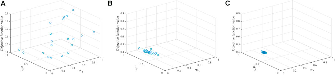
FIGURE 4. Distribution of gray wolf population in the GWO optimization process. (A) Initial population. (B) The sixtieth generation population. (C) The ninetieth generation population.

Subsequently, the ROC curve of the BP-SVM-RF model was generated. The ROC curves of every single model (BP, SVM, and RF) and integrated model of two models (BP-SVM, BP-RF, and SVM-RF) were also obtained for a comparison purpose (Figure 5). The AUC values were 0.7898 (BP-SVM-RF), 0.6929 (BP), 0.6582 (SVM), 0.7258 (RF), 0.7360 (BP-SVM), 0.7569 (BP-RF), and 0.7298 (SVM-RF), respectively. It can be seen that all the integrated models (BP-SVM-RF, BP-SVM, BP-RF, and SVM-RF) had a higher accuracy than that of individual model, and the BP-SVM-RF model was the best model. Hence, the integration of different machine learning models really improved the model performance.

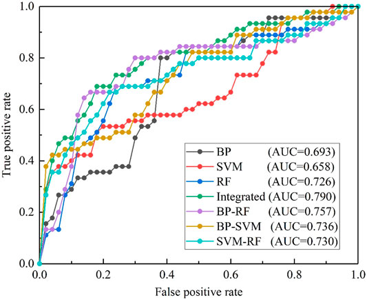
FIGURE 5. ROC curves of various models’ prediction results.

Landslide Susceptibility Mapping

The largest index value of landslide susceptibility in every grid was taken as the final index value of this grid, so as to achieve the prediction of regional landslide susceptibility index. The susceptibility index maps calculated by the seven models were imported into the ArcGIS, and the susceptibility index was divided into five levels (very low, low, medium, high, and very high) by using the geometric interval method to generate the final susceptibility map of the study area (Figure 6). It can be seen that the created landslide susceptibility maps by using different models had similar spatial pattern. The areas with very low and low susceptibility levels were distributed in flakes as a whole, while the areas with very high and high susceptibility were mainly distributed in linear clusters, which was consistent with the characteristics of historical landslide distribution. Most high susceptibility areas were distributed in the places with moderate slopes, low vegetation coverage, and low elevations. Moreover, more than 60% landslides were located in the range of plane curvature −1.3 to 1.14, and lithological units with loose geotechnical structure can also promote slope instability (Table 1). In high susceptibility areas, several residential areas, garden plots, and road network dense areas were mostly distributed here; thus human activities were more frequent. Hence, the combined effect of natural conditions and human activities posted higher landslide risks in the study area.

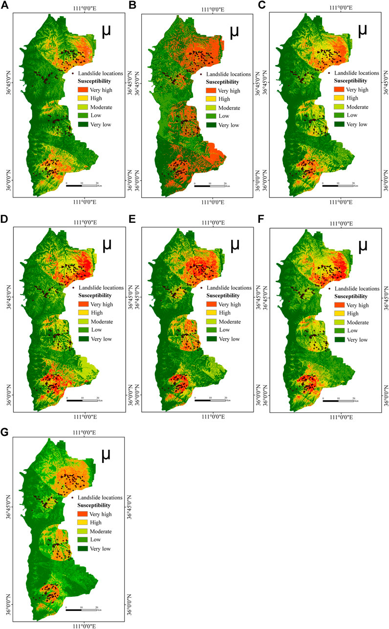
FIGURE 6. Landslide susceptibility maps respectively produced by different models: (A) BP, (B) SVM, (C) RF, (D) BP-SVM, (E) BP-RF, (F) SVM-RF, and (G) integrated BP-SVM-RF.

The evaluation results of the model fitting ability and generalization ability indicated that the BP-SVM-RF integrated model had a good prediction accuracy, but this performance measurement cannot reflect the spatial distribution pattern of the susceptibility index. To make the statistical analysis on the landslide distribution, the number of landslides, landslide percentages, grid numbers, and grid percentages of each susceptibility level were counted and landslide density was determined (Table 3). The results showed that most of the study area (65.85%) had low or very low susceptibility levels. 64.53% of landslides occurred in very high and high susceptibility areas, which could be considered to meet the requirements of spatial distribution verification accuracy. In addition, the landslide density, defined as the ratio of landslide percentage to susceptibility grade percentage, reflected the distribution information of historical landslides per unit area. With the increase of susceptibility level, landslide density increased correspondingly, which indicated that the evaluation result of the BP-SVM-RF integrated model was reasonable.

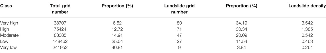
TABLE 3. Frequency ratios of five susceptibility classes assessed with the BP-SVM-RF model.

At last, all the sample data used in the modelling were reclassified into a binary of yes or no, and the results were shown as a confusion matrix (Table 4). All the models used 0.5 as the threshold of landslide susceptibility index. It can be seen that the performance of the BP-SVM-RF model was still the best. It has the highest TP and TN values, which indicated that the model accurately identified the most number of real landslide and nonlandslide points. In addition, the values of FP and FN of the BP-SVM-RF model were the lowest, thus showing its mis-reclassification was the lowest. Such analysis would be helpful for the decision making driven by management and allows the model to be compared to others that do a similar listing of results.

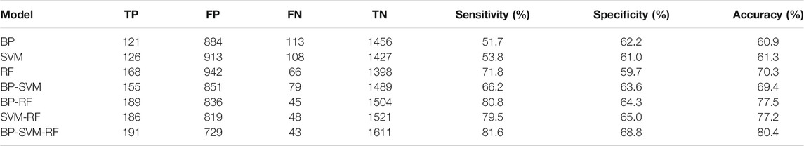
TABLE 4. Confusion matrix for classification results of different models.

Based on the results of the landslide susceptibility assessment, some suggestions can be provided to reduce and mitigate landslide risks in the study area:

1) The landslide susceptibility maps showed that the areas with low vegetation coverage were more susceptible to landslides. Hence, extensive afforestation should be encouraged, which can effectively improve the slope stability due to the root cohesion.

2) In low elevation areas, the human activities are more common, and slope stability can be more affected. Both Fr analysis and landslide susceptibility map showed that low-moderate elevations and moderate slope angles had more historical landslides. Hence, sufficient attention should be paid to these areas.

3) Most landslides in the area are composed of loess, which normally has weak geotechnical properties (e.g., sensitivity to water, and collapsibility). Hence, both engineering and agricultural activities should treat these properties cautiously when dealing with loess.

Discussion

Model Integration

Studies on generating regional landslide susceptibility maps based on the GIS platform are numerous and many of them have proposed suitable models for susceptibility assessment. A recent review stated that there were approximately 500 published papers which have used 70 models in the period of 2005–2016 (Pourghasemi et al., 2018). However, it should be noted that most studies were based on existing methods and tried to find better model by accuracy comparisons. Additionally, some studies so-called “integrated model” were not “real” integration of models. For example, Merghadi et al. (2020) used the convolutional neural network to extract features from landslide raw data and machine learning models were used to compute landslide susceptibility. Similar models and application procedures actually only used one model to achieve modelling. Hence, it is still highly encouraged to combine the outputs from different models to obtain “optimal” susceptibility maps for risk management and final decision making (Reichenbach et al., 2018). In fact, most available integrated models until now are related with different types of models, such as machine learning and statistical models. This is mainly because statistical techniques are normally required during the susceptibility modelling process, especially when analyzing the relationship between historical landslides and influencing factors (Fang et al., 2020). For instance, Guo et al. (2019) used weight of evidence method to analyze the effects of different factors on landslide occurrence and used the BP model to perform model training and prediction. Althuwaynee et al. (2016) applied the analytic hierarchy process to pairwise compare the CHAID terminal nodes to generate new landslide susceptibility maps. It can be seen that every single model was used to finish one specific task, which was not combined with other models.

In this study, all the three models were used to compute the landslide susceptibility index, and the final susceptibility for every cell contained three aspects. Hence, every single model directly affected the results, not only one specific step. The absolute value of the accuracy of the integrated model expressed by the ROC curve was not perfect, but it did improve the results compared with individual models. Such results supported the opinion that it is possible to combine different forecasts in an optimal prediction when multiple forecasts are available (Kocaman et al., 2020). This is mainly because the coupling model can combine the advantages of different models: The advantage of SVM is that high accuracy can be obtained on small sample training sets (Bui et al., 2016). The RF model can randomly select certain features as candidate features, and then the optimal features are selected. In this way, diversity of decision trees can be increased to improve the classification performance (Catani et al., 2013). The advantages of BP are the strong self-adaptive ability and good generalization (Guo et al., 2020). Last but not least, the three models were integrated by constructing an objective function in the present test. This can be also used for other machine learning models; thus the proposed procedure can be easily replicated into other case studies.

Selection of Causal Factors

As stated by Van Westen et al. (2006), one of the biggest difficulties in landslide susceptibility assessment is to find the best combination of environmental factors. In this study, we deleted five factors from the initial factor system based on expert’s opinion. This is a qualitative method which is subjective, but the subsequent test on the factor correlation showed that the correlations of the five factors with other factors were relatively high. Hence, the elimination of these factors made sense. However, the test on the model containing these factors would be still helpful, which was not available in the current analysis. Hence, it is recommended to use quantitative method to analyze the factor correlation and their contributions to the final results, such as forward (Pham et al., 2019) and backward elimination (Pham et al., 2016) methods and multicollinearity analysis (Lee et al., 2018).

Moreover, our objectives in the follow-up work also include the following:

i) More environmental factors should be considered into the analysis and more important factors should be selected for generating landslide susceptibility maps by calculating their importance quantitatively.

ii) The model application into other areas would be interesting. We will employ more machine learning models to verify the universality of the current procedure.

Conclusion

Various machine learning models are available for regional landslide susceptibility assessments, but few attempts have been made to integrate different models for better performances. In this study, three commonly used machine learning models (BP, SVM, and RF) were integrated into a model by constructing an objective function. The function computed the root mean square error between predicted and observed results, and the GWO algorithm was used to calculate the connecting weights among the three models. The test results in the Lvliang mountains of China showed that the integrated BP-SVM-RF model had a better accuracy with the AUC of 0.79, compared with every single model (AUC = 0.69 for BP, AUC = 0.67 for SVM, AUC = 0.73 for RF) and integrated model using two models (AUC = 0.74 for BP-SVM, AUC = 0.76 for BP-RF, AUC = 0.73 for SVM-RF). Hence, the proposed BP-SVM-RF model is an effective integrated model and suitable for landslide susceptibility assessment of the study area. Moreover, the GWO algorithm can be an option to integrate different models to seek “optimal” results.

Overall, the proposed procedure can be replicated into other landslide-prone areas, and different models can be selected as basic elements for the integrated model. Hence, the current results can guide the landslide risk mitigation of the study area, and they can also provide references for other case studies. The future work is to include more landslide-related influencing factors into the assessment and quantitatively express the importance of each factor.

Data Availability Statement

The data analyzed in this study is subject to the following licenses/restrictions: authors do not have permission to share data. Requests to access these datasets should be directed to YX, xingyin@hhu.edu.cn.

Author Contributions

YX contributed to writing of original draft, funding acquisition, and supervision. JY contributed to software, investigation, and writing review and editing. ZG contributed to methodology and supervision. YC contributed to project administration, investigation, and data curation. JH contributed to software, validation, and writing review and editing. AT contributed to writing review and editing.

Funding

This research was funded by the Postgraduate Research and Practice Innovation Program of Jiangsu Province (KYCX20_0484) and the Fundamental Research Funds for the Central Universities (B200203105) and the National Key Research and Development Program of China (2018YFC1508603).

Conflict of Interest

The authors declare that the research was conducted in the absence of any commercial or financial relationships that could be construed as a potential conflict of interest.

Publisher’s Note

All claims expressed in this article are solely those of the authors and do not necessarily represent those of their affiliated organizations, or those of the publisher, the editors and the reviewers. Any product that may be evaluated in this article, or claim that may be made by its manufacturer, is not guaranteed or endorsed by the publisher.

Acknowledgments

The authors would highly thank the Department of Surveying and Mapping of Shanxi Province for providing relevant data and the China Scholarship Council (202006710110).

References

Achour, Y., and Pourghasemi, H. R. (2020). How Do Machine Learning Techniques Help in Increasing Accuracy of Landslide Susceptibility Maps? Geosci. Front. 11, 871–883. doi:10.1016/j.gsf.2019.10.001
Aditian, A., Kubota, T., and Shinohara, Y. (2018). Comparison of GIS-Based Landslide Susceptibility Models Using Frequency Ratio, Logistic Regression, and Artificial Neural Network in a Tertiary Region of Ambon, Indonesia. Geomorphology 318, 101–111. doi:10.1016/j.geomorph.2018.06.006
Ahmed, B. (2015). Landslide Susceptibility Mapping Using Multi-Criteria Evaluation Techniques in Chittagong Metropolitan Area, Bangladesh. Landslides 12, 1077–1095. doi:10.1007/s10346-014-0521-x
Althuwaynee, O. F., Pradhan, B., and Lee, S. (2016). A Novel Integrated Model for Assessing Landslide Susceptibility Mapping Using CHAID and AHP Pair-wise Comparison. Int. J. Remote Sensing 37, 1190–1209. doi:10.1080/01431161.2016.1148282
Arabameri, A., Saha, S., Roy, J., Chen, W., Blaschke, T., and Tien Bui, D. (2020). Landslide Susceptibility Evaluation and Management Using Different Machine Learning Methods in the Gallicash River Watershed, Iran. Remote Sensing 12, 475. doi:10.1007/s12665-014-3661-310.3390/rs12030475
Ba, Q., Chen, Y., Deng, S., Yang, J., and Li, H. (2018). A Comparison of Slope Units and Grid Cells as Mapping Units for Landslide Susceptibility Assessment. Earth Sci. Inform. 11, 373–388. doi:10.1007/s12145-018-0335-9
Broeckx, J., Vanmaercke, M., Duchateau, R., and Poesen, J. (2018). A Data-Based Landslide Susceptibility Map of Africa. Earth-Science Rev. 185, 102–121. doi:10.1016/j.earscirev.2018.05.002
Bueechi, E., Klimeš, J., Frey, H., Huggel, C., Strozzi, T., and Cochachin, A. (2019). Regional-scale Landslide Susceptibility Modelling in the Cordillera Blanca, Peru-a Comparison of Different Approaches. Landslides 16, 395–407. doi:10.1007/s10346-018-1090-1
Bui, D. T., Tuan, T. A., Klempe, H., Pradhan, B., and Revhaug, I. (2016). Spatial Prediction Models for Shallow Landslide Hazards: a Comparative Assessment of the Efficacy of Support Vector Machines, Artificial Neural Networks, Kernel Logistic Regression, and Logistic Model Tree. Landslides 13, 361–378. doi:10.1007/s10346-015-0557-6.2016
Can, R., Kocaman, S., and Gokceoglu, C. (2021). A Comprehensive Assessment of XGBoost Algorithm for Landslide Susceptibility Mapping in the Upper Basin of Ataturk Dam, Turkey. Appl. Sci. 11 (11), 4993. available at: https://www.mdpi.com/2076-3417/11/11/4993. doi:10.3390/app11114993
Cantarino, I., Carrion, M. A., Goerlich, F., and Martinez Ibañez, V. (2019). A ROC Analysis-Based Classification Method for Landslide Susceptibility Maps. Landslides 16, 265–282. doi:10.1007/s10346-018-1063-4
Castellanos Abella, E. A., and Van Westen, C. J. (2008). Qualitative landslide susceptibility assessment by multicriteria analysis: A case study from San Antonio del Sur, Guantánamo, Cuba. Geomorphology 94, 453–466. doi:10.1016/j.geomorph.2006.10.038
Catani, F., Lagomarsino, D., Segoni, S., and Tofani, V. (2013). Landslide Susceptibility Estimation by Random Forests Technique: Sensitivity and Scaling Issues. Nat. Hazards Earth Syst. Sci.Hazards Earth Syst. Sci. 13, 2815–2831. doi:10.5194/nhess-13-2815-2013
Chang, Z., Du, Z., Zhang, F., Huang, F., Chen, J., Li, W., et al. (2020). Landslide Susceptibility Prediction Based on Remote Sensing Images and GIS: Comparisons of Supervised and Unsupervised Machine Learning Models. Remote Sensing 12, 502. doi:10.3390/rs12030502
Chen, L., Guo, Z., Yin, K., Shrestha, D. P., and Jin, S. (2019). The influence of land use and land cover change on landslide susceptibility: a case study in Zhushan Town, Xuan'en County (Hubei, China). Nat. Hazards Earth Syst. Sci. 19, 2207–2228. doi:10.16031/j.cnki.issn.1003-8035.2019.01.0610.5194/nhess-19-2207-2019
Chen, T., Trinder, J., and Niu, R. (2017). Object-oriented Landslide Mapping Using ZY-3 Satellite Imagery, Random forest and Mathematical Morphology, for the Three-Gorges Reservoir, China. Remote Sensing 9, 333. doi:10.3390/rs9040333
Chen, W., and Li, Y. (2020). GIS-based Evaluation of Landslide Susceptibility Using Hybrid Computational Intelligence Models. Catena 195, 104777. doi:10.1016/j.catena.2020.104777
Chen, W., Pourghasemi, H. R., Kornejady, A., and Zhang, N. (2017). Landslide Spatial Modeling: Introducing New Ensembles of ANN, MaxEnt, and SVM Machine Learning Techniques. Geoderma 305, 314–327. doi:10.1016/j.geoderma.2017.06.020
Chen, W., Xie, X., Wang, J., Pradhan, B., Hong, H., Bui, D. T., et al. (2017). A Comparative Study of Logistic Model Tree, Random forest, and Classification and Regression Tree Models for Spatial Prediction of Landslide Susceptibility. Catena 151, 147–160. doi:10.1016/j.catena.2016.11.032
Corsini, A., and Mulas, M. (2017). Use of ROC Curves for Early Warning of Landslide Displacement Rates in Response to Precipitation (Piagneto Landslide, Northern Apennines, Italy). Landslides 14, 1241–1252. doi:10.1007/s10346-016-0781-8
Crippa, P., Sullivan, R. C., Thota, A., and Pryor, S. C. (2016). Evaluating the Skill of High-Resolution WRF-Chem Simulations in Describing Drivers of Aerosol Direct Climate Forcing on the Regional Scale. Atmos. Chem. Phys. 16 (1), 397–416. doi:10.5194/acp-16-397-2016
Cruden, D. M., and Varnes, D. J. (1996). “Landslide Types and Processes,” in Landslides Investigation and Mitigation. Editors A. K. Turner, and R. L. Schuster (Washington, DC: Transportation research board. US National Research Council. Special Report 247), 36–75.
Cuomo, S., and Della Sala, M. (2015). Large-area Analysis of Soil Erosion and Landslides Induced by Rainfall: A Case of Unsaturated Shallow Deposits. J. Mt. Sci. 12, 783–796. doi:10.1007/s11629-014-3242-7
Derbyshire, E. (2001). Geological Hazards in Loess Terrain, with Particular Reference to the Loess Regions of China. Earth-Science Rev. 54, 231–260. doi:10.1016/S0012-8252(01)00050-2
Ermini, L., Catani, F., and Casagli, N. (2005). Artificial Neural Networks Applied to Landslide Susceptibility Assessment. Geomorphology 66, 327–343. doi:10.1016/j.geomorph.2004.09.025
Fang, Z., Wang, Y., Peng, L., and Hong, H. (2020). Integration of Convolutional Neural Network and Conventional Machine Learning Classifiers for Landslide Susceptibility Mapping. Comput. Geosciences 139, 104470. doi:10.1016/j.cageo.2020.104470
Fell, R., Corominas, J., Bonnard, C., Cascini, L., Leroi, E., and Savage, W. Z. (2008). Guidelines for Landslide Susceptibility, hazard and Risk Zoning for Land Use Planning. Eng. Geology. 102, 85–98. doi:10.1016/j.enggeo.2008.03.01410.1016/j.enggeo.2008.03.022
Goetz, J. N., Brenning, A., Petschko, H., and Leopold, P. (2015). Evaluating Machine Learning and Statistical Prediction Techniques for Landslide Susceptibility Modeling. Comput. Geosciences 81, 1–11. doi:10.1016/j.cageo.2015.04.007
Guo, Z., Chen, L., Gui, L., Du, J., Yin, K., and Do, H. M. (2020). Landslide Displacement Prediction Based on Variational Mode Decomposition and WA-GWO-BP Model. Landslides 17, 567–583. doi:10.1007/s10346-019-01314-4
Guo, Z., Yin, K., Fu, S., Huang, F. M., Gui, L., and Xia, H. (2019). Evaluation of Landslides Susceptibility Based on GIS and WOE-BP Model. Earth Sci. 44, 4299–4312. doi:10.3799/dqkx.2018.555
Guo, Z., Yin, K., Huang, F., and Liang, X. (2018). Landslide Displacement Prediction Based on Surface Monitoring Data and Nonlinear Time Series Combination Model. Chin. J. Rock Mech Eng. 37, 3392–3399. doi:10.13722/j.cnki.jrme.2016.1534
Guzzetti, F., Carrara, A., Cardinali, M., and Reichenbach, P. (1999). Landslide hazard Evaluation: a Review of Current Techniques and Their Application in a Multi-Scale Study, Central Italy. Geomorphology 31, 181–216. doi:10.1016/S0169-555X(99)00078-1
Guzzetti, F., Reichenbach, P., Ardizzone, F., Cardinali, M., and Galli, M. (2006). Estimating the Quality of Landslide Susceptibility Models. Geomorphology 81, 166–184. doi:10.1016/j.geomorph.2006.04.007
Huang, F., Cao, Z., Guo, J., Jiang, S.-H., Li, S., and Guo, Z. (2020). Comparisons of Heuristic, General Statistical and Machine Learning Models for Landslide Susceptibility Prediction and Mapping. Catena 191, 104580. doi:10.1016/j.catena.2020.104580
Huang, F., Yin, K., Huang, J., Gui, L., and Wang, P. (2017). Landslide Susceptibility Mapping Based on Self-Organizing-Map Network and Extreme Learning Machine. Eng. Geology. 223, 11–22. doi:10.1016/j.enggeo.2017.04.013
Hungr, O., Leroueil, S., and Picarelli, L. (2014). The Varnes Classification of Landslide Types, an Updatefication of Landslide Types, an Update. Landslides 11, 167–194. doi:10.1007/s10346-013-0436-y
King, G., and Zeng, L. (2001). Logistic Regression in Rare Events Data. Polit. Anal. 9, 137–163. doi:10.1093/oxfordjournals.pan.a004868
Klimešl, J., Stemberk, J., Blahut, J., Krejčí, V., Krejčí, O., Hartvich, F., et al. (2017). Challenges for Landslide hazard and Risk Management in ‘low-Risk’ Regions, Czech Republic—landslide Occurrences and Related Costs (IPL Project No. 197). Landslides 14, 771–780. doi:10.1007/s10346-017-0798-7
Kocaman, S., Tavus, B., Nefeslioglu, H. A., Karakas, G., and Gokceoglu, C. (2020). Evaluation of Floods and Landslides Triggered by a Meteorological Catastrophe (Ordu, Turkey, August 2018) Using Optical and Radar Data. Ordu, Turkey: Geofluids, 8830661. doi:10.1155/2020/8830661 available at: https://www.hindawi.com/journals/geofluids/2020/8830661/.
Lee, J.-H., Sameen, M. I., Pradhan, B., and Park, H.-J. (2018). Modeling Landslide Susceptibility in Data-Scarce Environments Using Optimized Data Mining and Statistical Methods. Geomorphology 303, 284–298. doi:10.1016/j.geomorph.2017.12.007
Medina, V., Hürlimann, M., Guo, Z., Lloret, A., and Vaunat, J. (2021). Fast Physically-Based Model for Rainfall-Induced Landslide Susceptibility Assessment at Regional Scale. Catena 201, 105213. doi:10.1016/j.catena.2021.105213
Merghadi, A., Yunus, A. P., Dou, J., Whiteley, J., ThaiPham, B., Bui, D. T., et al. (2020). Machine Learning Methods for Landslide Susceptibility Studies: A Comparative Overview of Algorithm Performance. Earth-Science Rev. 207, 103225. doi:10.1016/j.earscirev.2020.103225
Mirjalili, S. (2015). How Effective Is the Grey Wolf Optimizer in Training Multi-Layer Perceptrons. Appl. Intell. 43, 150–161. doi:10.1007/s10489-014-0645-7
Mirjalili, S., Mirjalili, S. M., and Lewis, A. (2013). Grey Wolf Optimizer. Adv. Eng. Softw. 69, 46–61. doi:10.1016/j.advengsoft.12.0072014
Nam, K., and Wang, F. (2019). The Performance of Using an Autoencoder for Prediction and Susceptibility Assessment of Landslides: A Case Study on Landslides Triggered by the 2018 Hokkaido Eastern Iburi Earthquake in Japan. Geoenviron Disasters 6, 19. doi:10.1186/s40677-019-0137-5
Pereira, S., Zêzere, J. L., and Bateira, C. (2012). Technical Note: Assessing Predictive Capacity and Conditional independence of Landslide Predisposing Factors for Shallow Landslide Susceptibility Models. Nat. Hazards Earth Syst. Sci. 12, 979–988. doi:10.5194/nhess-12-979-2012
Petley, D. (2012). Global Patterns of Loss of Life from Landslides. Geology 40, 927–930. doi:10.1130/G33217.1
Pham, B. T., Jaafari, A., Prakash, I., and Bui, D. T. (2019). A Novel Hybrid Intelligent Model of Support Vector Machines and the MultiBoost Ensemble for Landslide Susceptibility Modeling. Bull. Eng. Geol. Environ. 78, 2865–2886. doi:10.1007/s10064-018-1281-y
Pham, B. T., Pradhan, B., Tien Bui, D., Prakash, I., and Dholakia, M. B. (2016). A Comparative Study of Different Machine Learning Methods for Landslide Susceptibility Assessment: a Case Study of Uttarakhand Area (India). Environ. Model. Softw. 84, 240–250. doi:10.1016/j.envsoft.2016.07.005
Pham, B. T., Tien Bui, D., Prakash, I., and Dholakia, M. B. (2017). Hybrid Integration of Multilayer Perceptron Neural Networks and Machine Learning Ensembles for Landslide Susceptibility Assessment at Himalayan Area (India) Using GIS. Catena 149, 52–63. doi:10.1016/j.catena.2016.09.007
Pourghasemi, H. R., Teimoori Yansari, Z., Panagos, P., and Pradhan, B. (2018). Analysis and Evaluation of Landslide Susceptibility: a Review on Articles Published during 2005-2016 (Periods of 2005-2012 and 2013-2016). Arab J. Geosci. 11, 1–12. doi:10.1007/s12517-018-3531-5
Reichenbach, P., Rossi, M., Malamud, B. D., Mihir, M., and Guzzetti, F. (2018). A Review of Statistically-Based Landslide Susceptibility Models. Earth-Science Rev. 180, 60–91. doi:10.1016/j.earscirev.2018.03.001
Rossi, M., Guzzetti, F., Reichenbach, P., Mondini, A. C., and Peruccacci, S. (2010). Optimal Landslide Susceptibility Zonation Based on Multiple Forecasts. Geomorphology 114, 129–142. doi:10.1016/j.geomorph.2009.06.020
Segoni, S., Rossi, G., and Catani, F. (2012). Improving basin Scale Shallow Landslide Modelling Using Reliable Soil Thickness Maps. Nat. Hazards. 61, 85–101. doi:10.1007/s11069-011-9770-10.1007/s11069-011-9770-3
Sevgen, E., Kocaman, S., Nefeslioglu, H. A., and Gokceoglu, C. (2019). A Novel Performance Assessment Approach Using Photogrammetric Techniques for Landslide Susceptibility Mapping with Logistic Regression, ANN and Random Forest. Sensors 19 (18), 3940. doi:10.3390/s19183940
Sezer, E. A., Nefeslioglu, H. A., and Osna, T. (2017). An Expert-Based Landslide Susceptibility Mapping (LSM) Module Developed for Netcad Architect Software. Comput. Geosciences 98, 26–37. doi:10.1016/j.cageo.2016.10.001
Shrestha, D. P., Zinck, J. A., and Van Ranst, E. (2004). Modelling Land Degradation in the Nepalese Himalaya. Catena 57, 135–156. doi:10.1016/j.catena.2003.11.003
Shu, H., Hürlimann, M., Molowny-Horas, R., González, M., Pinyol, J., Abancó, C., et al. (2019). Relation between Land Cover and Landslide Susceptibility in Val d'Aran, Pyrenees (Spain): Historical Aspects, Present Situation and Forward Prediction. Sci. Total Environ. 693, 133557. doi:10.1016/j.scitotenv.2019.07.363
Tang, Y., Feng, F., Guo, Z., Feng, W., Li, Z., Wang, J., et al. (2020). Integrating Principal Component Analysis with Statistically-Based Models for Analysis of Causal Factors and Landslide Susceptibility Mapping: A Comparative Study from the Loess Plateau Area in Shanxi (China). J. Clean. Prod. 277, 124159. doi:10.1016/j.jclepro.2020.124159
Tian, Y., Xu, C., Ma, S., Xu, X., Wang, S., and Zhang, H. (2019). Inventory and Spatial Distribution of Landslides Triggered by the 8th August 2017 MW 6.5 Jiuzhaigou Earthquake, China. J. Earth Sci. 30, 206–217. doi:10.1007/s12583-018-0869-2
Tofani, V., Bicocchi, G., Rossi, G., Segoni, S., D’Ambrosio, M., Casagli, N., et al. (2017). Soil Characterization for Shallow Landslides Modeling: a Case Study in the Northern Apennines (Central Italy). Landslides 14, 755–770. doi:10.1007/s10346-017-0809-8
Van Westen, C. J., Castellanos, E., and Kuriakose, S. L. (2008). Spatial Data for Landslide Susceptibility, hazard, and Vulnerability Assessment: An Overview. Eng. Geology. 102, 112–131. doi:10.1016/j.enggeo.2008.03.010
Van Westen, C. J., Rengers, N., and Soeters, R. (2003). Use of Geomorphological Information in Indirect Landslide Susceptibility Assessment. Nat. Hazards 30, 399–419. doi:10.1023/B:NHAZ.0000007097.42735.9e
Van Westen, C. J., Van Asch, T. W. J., and Soeters, R. (2006). Landslide hazard and Risk Zonation-Why Is it Still So Difficult? Bull. Eng. Geol. Environ. 65, 167–184. doi:10.1007/s10064-005-0023-0
Wang, J.-J., Liang, Y., Zhang, H.-P., Wu, Y., and Lin, X. (2014). A Loess Landslide Induced by Excavation and Rainfall. Landslides 11, 141–152. doi:10.1007/s10346-013-0418-0
Wang, J., Zhang, D., Wang, N., and Gu, T. (2019). Mechanisms of Wetting-Induced Loess Slope Failures. Landslides 16, 937–953. doi:10.1007/s10346-019-01144-4
Youssef, A. M., Pradhan, B., Jebur, M. N., and El-Harbi, H. M. (2015). Landslide Susceptibility Mapping Using Ensemble Bivariate and Multivariate Statistical Models in Fayfa Area, Saudi Arabia. Environ. Earth Sci. 73, 3745–3761. doi:10.1007/s12665-014-3661-3
Zhuang, J.-q., and Peng, J.-b. (2014). A Coupled Slope Cutting-A Prolonged Rainfall-Induced Loess Landslide: a 17 October 2011 Case Study. Bull. Eng. Geol. Environ. 73, 997–1011. doi:10.1007/s10064-014-0645-1
Keywords: landslide susceptibility, random forest, integrated model, causal factor, GIS
Citation: Xing Y, Yue J, Guo Z, Chen Y, Hu J and Travé A (2021) Large-Scale Landslide Susceptibility Mapping Using an Integrated Machine Learning Model: A Case Study in the Lvliang Mountains of China. Front. Earth Sci. 9:722491. doi: 10.3389/feart.2021.722491
Received: 08 June 2021; Accepted: 08 July 2021;
Published: 17 August 2021.
Edited by:
Faming Huang, Nanchang University, ChinaReviewed by:
Candan Gokceoglu, Hacettepe University, TurkeyYangyang Mo, Universitat Politecnica de Catalunya, Spain
Zhou Ye, Nanchang University, China
Copyright © 2021 Xing, Yue, Guo, Chen, Hu and Travé. This is an open-access article distributed under the terms of the Creative Commons Attribution License (CC BY). The use, distribution or reproduction in other forums is permitted, provided the original author(s) and the copyright owner(s) are credited and that the original publication in this journal is cited, in accordance with accepted academic practice. No use, distribution or reproduction is permitted which does not comply with these terms.
*Correspondence: Zizheng Guo, cuggzz@cug.edu.cn