Time-Varying Impact of Economic Growth on Carbon Emission in BRICS Countries: New Evidence From Wavelet Analysis

Introduction

The climate change has been deemed as one of the most urgent issues that are confronted by the humankind. It results in far-reaching and complex socioeconomic consequences (Dai et al., 2016; Dottori et al., 2018; Pinsky et al., 2019). So far, a global consensus has been reached that the greenhouse gas, especially CO2, causes climate change. Facing the threat of global warming to economic prosperity and sustainability, the carbon emission reduction measures have been proposed as a response.

World economy is fueled largely by the fossil energy sources. The dilemma of environmental degradation and economic growth needs to be handled to optimize the human welfare. The decoupling indexes reflect a variety of different coupling states of carbon emission and economic growth in the literature (Gao et al., 2015). Although this approach provides real-time measure for the relationship between carbon emission and economic growth, the influence from other important factors is left out of consideration. As a result, the decoupling analysis fails to reveal the time-varying real effect of economic growth on carbon emission and to identify the evolving impact from other crucial factors.

Besides the studies that have investigated the relationship between economic growth and carbon emission, much attention has been paid on the impact of energy transition and international trade on emission emerges. That is because not only the quantity of production output (GDP), but also the change in energy sources and production distribution worldwide, which can be proxied by energy structure and trade openness respectively, pose a significant impact on carbon emission. Energy is a critical input to economic development and an essential part of human activity. The current world energy consumption is mainly based on fossil fuel energy. Thus, the research on energy transition is of practical importance (Wang and Wang, 2020). In the process of globalization, there is no doubt that the change in one country’s level of trade openness will reshape its production distribution and industrial emission structure (Wang and Zhang, 2021). Therefore, it is necessary to incorporate variables that represent both the economic output itself and the way to achieve it into the model.

The BRICS countries (Brazil, Russia, India, China, and South Africa) are experiencing drastic economic transition and structural change. The shifts in their energy structure and level of trade openness are profound and influencing, which makes them excellent samples for empirical investigation. This article attaches importance to the effects of energy structure and trade openness on carbon emission along with the economic growth. Based on results from decoupling analysis, the continuous wavelet analysis framework is applied to dig deeper into the complex relationships among carbon emission and economic growth.

The contribution of this article to the extant literature is as follows: 1) the application of wavelet transform allows us to estimate partial phase-difference to depict both the short-term (high-frequency) and long-term (low-frequency) causality between economic growth and carbon emission. The relationship changes over time and across frequencies. Our analysis advances the analysis of the decoupling states to the identification of causality; 2) the wavelet analysis framework is extended to estimate the magnitude of marginal impact of economic growth on carbon emission by introducing the (partial) wavelet gain. Compared with previous studies, the interference from other factors is suppressed. And the applied wavelet model generates much richer empirical results including correlation, causality, and statistics that measure magnitude of marginal impact; 3) The physical inputs, including capital and labor, and the proxy of economic development have been introduced into the estimation to examine whether the newly developed wavelet analysis approach is able to overcome the omitted variable bias documented in the literature; 4) The wavelet analysis approach captures the nonlinear dynamics among economic variables. In addition to the decoupling states, more dynamic characteristics and evolving patterns can be inferred from our estimated statistics such that the conclusions drawn from the empirical results provide a deeper understanding of the time-varying impact of economic growth on carbon emission.

The remainder of the article is organized as follows. Literature Review Section reviews the relevant literature and presents the motivation and contribution. In Methodology Section the methodology is introduced in detail. Data and Empirical Results Section presents the data and empirical result. Then in the last section, we draw conclusion and provide corresponding policy implication.

Literature Review

Along with economic development, environmental degradation problems gradually emerge. Many researchers believe that there is a close relationship between economic development and carbon emissions (e.g., Selden and Song, 1994; Galeotti et al., 2009; Saboori et al., 2012). Extensive studies have begun to focus on the relationship between GDP growth and carbon dioxide emissions based on testing the effectiveness of environmental Kuznets curve (EKC) in different countries and regions (Apergis, 2016; Apergis et al., 2017; Murshed, 2020; Murshed et al., 2021a; Murshed et al., 2021b).

Scholars draw different conclusions on the relationship between GDP growth and energy consumption using Granger causality. The results from the Granger causality tests suggest that in the long run there is unidirectional Granger causality running from electricity consumption and emissions to economic growth (Lean and Smyth, 2010). Apergis and Tang (2013) reexamine the validity of the energy-led growth hypothesis using different model specifications. Compared with the Granger causality model containing only two variables, the Granger causality model containing three and four variables is more likely to support the assumption. In addition, both developed and developing countries are more likely to support the energy-led growth assumption than less developed or low-income countries.

There are many factors affecting carbon emissions. Scholars have conducted different analyses and found some major factors. Banerjee and Murshed (2020) confirmed the pollution paradise hypothesis by examining cross-sectional dependencies between national teams in 2005–2015 and determining the long-term equilibrium relationship between net export emissions and real GDP, FDI, trade openness, energy consumption, and financial development. Murshed (2020) drew a conclusion that in South Asia ICT trade reduces CO2 emissions by directly increasing renewable energy consumption, increasing the share of renewable energy, reducing energy intensity, promoting cleaner cooking fuels, indirectly increasing the level of renewable energy consumption, improving energy efficiency, and strengthening cleaner cooking fuel channels. In addition, environmental policy is also an important influencing factor. From an environmental perspective there is potential to use pricing policies in the G7 countries to curtail residential electricity demand, and thus curb carbon emissions, in the long run (Narayan et al., 2007).

In the case of China, Ma et al. (2021) find that provincial growth and the development of the tertiary industry are the reasons for the deterioration of China's carbon dioxide emission trend. The survey results also show that emission taxes, investment in research and development, technological innovation, and the use of renewable energy together further reduce carbon dioxide emission. Abdul et al. (2021) indicated that the positive impact on grain crop production will only increase carbon dioxide emissions in the long term, the impact on forestry will not have any significant impact on China's carbon dioxide emissions level, and the negative impact on livestock production will only increase carbon dioxide emissions in the short term.

Decoupling of Economic Growth and Carbon Emission

The decoupling analysis framework was proposed to confirm the disconnection between economic growth and environmental degradation (Tapio, 2005). It has been widely applied to various levels (Wang and Zhang, 2020). Compared with the Environmental Kuznets Curve framework, decoupling analysis is straightforward and able to reveal the real-time relationship in different horizons (Dong et al., 2020). The rationale of decoupling analysis is to dissociate economic growth from environmental degradation to achieve sustainable development (Zhang and Zhang, 2020). It provides a way to perform decomposition on the complex relationship between two variables. Many scholars address the dilemma of economic growth and environmental degradation using the decoupling framework and make significant progresses (Csereklyei and Stern, 2015; Kovanda and Hak, 2007; Loo and Banister, 2016).

Dai et al. (2016) identified decoupling state of BRICS countries and further explored driving factors on decoupling. Some scholars conduct decomposition and decoupling analysis of carbon dioxide emissions from economic growth in China and the ASEAN countries (Zhang et al., 2020). Another study took the Belt and Road as the starting point to analyze spatiotem poral evolution of decoupling and driving forces of CO2 emissions on economic growth (Hu et al., 2020). Adedoyin et al. (2020) introduced coal rents vs coal consumption and other energy sources as determinants of CO2 emissions in BRICS economies. Wang and Zhang (2020) studied the influence of increasing investment in research and development on economic growth decoupling from carbon emission. Wang and Wang (2020) discovered the promoting effect of energy transition on the decoupling economic growth from emission. Nandini and Joyashree (2020) decomposed energy-related CO2 emissions, using LMDI approach, to quantify drivers of climate change. And decoupling elasticity is estimated to identify historical attainment in decoupling economic growth from emissions in India.

Energy Structure and Carbon Emission

Energy is essential material input for production. Economic growth cannot sustain without enough energy consumption. Hence, intuitively, energy consumption should maintain a long-term equilibrium with economic growth (Zhang, 2011). Adedoyin et al. (2020) find that the BRICS countries are heavily dependent on energy-intensive sectors such as construction, mining, and manufacturing, because of a rapid increase in population, lifestyle changes, and urbanization. It is a natural choice to achieve emission reduction by improving energy efficiency. Guan et al. (2018) find that the most important factor in reducing carbon emissions in China is the improvement of energy efficiency, during the sample period from 2007 to 2010.

Among the factors affecting carbon emissions, energy consumption is one of the most important factors and energy consumption has different effects in countries with different development status. The results show that the United States strongly supports the hypothesis of neutrality. While a developing economy panel (90 countries) favors the conservative hypothesis, and a panel of 32 lower middle-income countries suggests that energy consumption per capita predicts real GDP per capita (Narayan, 2016). Narayan and Smyth (2007) suggest that the demand for oil in the Middle East is being driven largely by strong economic growth. In the near future, Malaysia’s energy import dependency will rise. Carbon emissions will triple by 2030 (Gan and Li, 2008). New energy and renewable energy have become the focus in the energy consumption–growth relationship research (Apergis and Payne, 2010a; Apergis and Payne, 2010b; Apergis et al., 2010; Apergis and Payne, 2011a; Apergis and Payne, 2011b; Apergis and Payne, 2012; Murshed et al., 2021). Thus, it is necessary to incorporate an energy structure in the empirical study of growth–carbon emission relationship.

When the marginal carbon reduction effect of energy efficiency improvement gradually reaches its ceiling, renewable energy turns out to be a more promising alternative. Energy transition has caught much attention and has been regarded as an efficient approach to reduce carbon emission and achieve low-carbon development (Obama, 2017; Wang and Su, 2020). International Energy Agency (IEA) carried out the Clean Energy Transitions Program (CETP) to facilitate global energy transition¹. IEA demonstrated that energy transition can enhance energy security, robust energy system at the same time thrive economy in its annual report2018².

For the developing countries, scholars find that increasing the share of renewable energy use could reduce emission (Liu et al., 2017; Hu et al., 2018). The recent research found that renewable energy decreases CO2 emissions in African countries (Dauda et al., 2021). Fragkos et al. (2021) investigate Energy system transitions and low-carbon pathways. Their results imply the technical-economic feasibility of achieving large emission reductions by 2050.

Trade Openness and Carbon Emission

Trade liberalization has significantly reshaped industries and production network worldwide. Since the seminal work by Grossman and Krueger (1991), many scholars have attempted to examine the effect of trade openness on the environment.

Since countries experience different levels of income and foreign trade depending on their level of economic development, the relationship between emissions and trade depends on where an economy is currently placed in its development trajectory (Baek et al., 2009). Antweiler et al. (2001) have systematically described three major categories of the impact on the environment, namely the scale, technique, and composition effects. They point out that the technique effect overshadows the scale effect.

The debate regarding the relationship between trade openness and environmental degradation has not reached a consensus yet. The findings based on the different methodology and data are quite discrepant (Cole and Elliott, 2003; Frankel and Rose, 2005; Managi et al., 2008). Copeland and Taylor (2003), Tiba et al. (2015), and Tiba and Frikha (2018), among others, revealed the existence of a significant positive impact of trade openness on environmental quality. In constant, Salman et al. (2019) found that export increases CO2 emissions in some countries in Asia after disaggregating trade into export and import. The relationship between trade openness and carbon emissions still merits further investigation (Wang and Zhang, 2021).

This article uses data from the BRICS countries to explore the dynamic relationship between carbon emission and economic growth. Decoupling approach is introduced to reflect the states of growth–emission nexus. And based on that, the wavelet analysis is applied to provide deeper insight and extensive discussion on the impact of economic growth on carbon emission.

Methodology

Tapio Decoupling Model

In this article, we adopt the decoupling approach that is being widely used in the literature to provide a portrait for the complex growth–emission relationship. The OECD decoupling index (de Freitas and Kaneko, 2011; Yu et al., 2013; Zhao et al., 2017), the Tapio decoupling model (Climent and Pardo, 2007; Dong et al., 2016; Kan et al., 2019; Roman-Collado et al., 2018; Sorrell et al., 2012; Tapio, 2005; Zhang et al., 2015), the IGTX decoupling method (Ma et al., 2016), and the EA method (Enevoldsen et al., 2007; Mielnik and Goldemberg, 2002) are four alternative approaches for analyzing economic growth decoupling from environmental pollution. Since the Tapio (2005) method is most widely applied in the literature, we follow this approach to define the decoupling elasticity as:

where $e\left(C\right)$ indicates the decoupling elasticity coefficient between economic activities and carbon emissions, $\Delta C$ and $\Delta G$ respectively indicate the total carbon emission change and the total GDP change from the base period to the end period. $C_0$ indicates the carbon emissions at the base period, and $G_0$ indicates the base period GDP.

As shown in Figure 1, in the first quadrant, both carbon emission and GDP increase simultaneously, represent expansive negative decoupling; $0.8\le e\le 1.2$ represents expansive coupling; $0\le e<0.8$ represents weak decoupling. While in the third quadrant, both carbon emission and GDP decrease simultaneously, $e>1.2$ represents recessive decoupling; $0.8\le e\le 1.2$ represents recessive coupling; $0\le e<0.8$ represents weak negative decoupling. In the second and fourth quadrants, $e<0$ represent that carbon emission and GDP change asynchronously. In the fourth quadrant, there is strong decoupling, the best decoupling state, indicating economy increasing while carbon emission decreasing. In the second quadrant, it is strong negative decoupling, the worst decoupling state, showing economy decreasing while carbon emission increasing.

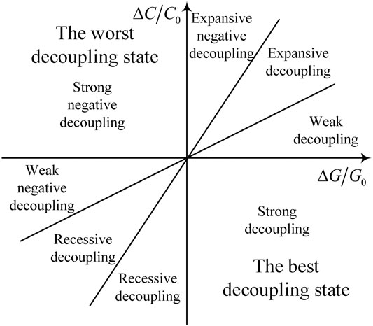
FIGURE 1. chematic diagram of decoupling states.

Wavelet Model

To carry out further in-depth research, we introduce the wavelet analysis framework. The wavelet model is an extension of spectral analysis (Mandler and Scharnagl, 2014). Wavelet analysis can reveal the frequency components of variables just like the Fourier transform, in addition to extraction of series characteristics in the time domain. It is a sophisticated time-frequency analysis technique that outperforms pure time series or frequency domain methods. As a result, it has been widely used for data processing and econometric analysis. While the Fourier transform breaks down a time series into constituent sinusoids of different frequencies and infinite duration in time, the wavelet transform expands the time series into shifted and scaled versions of a function, the so-called mother wavelet, that has limited spectral band and limited duration in time (Aguiar-Conraria et al., 2018).

Continuous Wavelet Transform

Discrete wavelet transform (DWT) and continuous wavelet transform (CWT) are two classes of wavelet transform. The DWT is useful for noise reduction and data compression, while the CWT is more helpful for feature extraction and data self-similarity detection (Grinsted et al., 2004; Loh, 2013). In application, continuous wavelet transformation is often chosen to extract the characteristics of economic variables and perform correlation and causality analysis. This approach utilizes information from two dimensions, namely time and frequency. Thus, it is suffered less estimation bias other than empirical methods developed to identify economic relationship solely in the time domain.

Assuming the mother wavelet function is $\psi \left(t\right)$, the corresponding base wavelet function is

where $\tau$ is the translation factor, which represents the magnitude of the mother wavelet function's translation, and different values will produce different window positions. $s$ is the expansion factor, which represents the degree of expansion of the mother wavelet function. When the $s$ is less than 1, the function is compressed, which is beneficial to capture the high-frequency part of original sequence, and when the $s$ is greater than 1, the function is stretched, which is beneficial to capture the low-frequency part. By changing the two parameters, one can construct a picture showing how the amplitudes of $x\left(t\right)$ vary across scales and how such amplitudes change over time (Torrence and Compo, 1998).

A continuous wavelet transformation can be expressed as follows:

Because of the need for both amplitude and phase information, it is necessary to select complex wavelet, and the Morlet wavelet satisfies this condition. Based on the Morlet continuous wavelet transform, we can calculate (partial) wavelet coherency, (partial) phase-difference, and (partial) wavelet gain to analyze the correlation and causality relationship between two or more time series and the magnitude of the impact.

Wavelet Coherency and Phase-Difference

In analogy with the terminology used in the Fourier case, the local wavelet power spectrum of the time series is defined as $|W_x\left(\tau ,s\right){|}^2$, which measures the magnitude of the time series fluctuation in the time-frequency space. The wavelet power spectrum may be averaged over time for comparison with classical spectral methods. When the average is taken over all times, we obtain the global wavelet power spectrum as follows:

For two time series $x\left(t\right)$ and $y\left(t\right)$, we can obtain the cross-wavelet transform corresponding to$\left(\tau ,s\right)$:

And the corresponding cross-wavelet power spectrum is as follows:

where $W_y^{\ast }\left(\tau ,s\right)$ represents the complex conjugate of the continuous wavelet transform function.

Following Torrence & Webster (1999), the Wavelet Coherence of two time series is defined as:

where$S$is the smoothing operator.

According to Bloomfield et al. (2004), the wavelet phase-difference enables us to calculate the phase of the wavelet transform of each time series. And wavelet phase-difference is defined as follows:

where $\Im$ and $\Re$ are the imaginary and real parts of the smoothed cross-wavelet transform, respectively. Using the phase-difference, the time lag or time difference, which gives the lead or lag of the series in the time domain, can be calculated as $\Delta T_n\left(s\right)={\phi }_n\left(s\right)/\omega$, where $\omega$ is the angular frequency with respect to the time scale.

When the phase-difference falls in different quadrants, it represents different types of correlations and causality relationships between variables, as shown in Figure 2. As referred to partial phase-difference, it indicates the time-varying correlations and causality relationships between two variables after controlling other factors. By its nature, this indicator can precisely capture the sign of correlation and the direction of causality over time and across different frequencies.

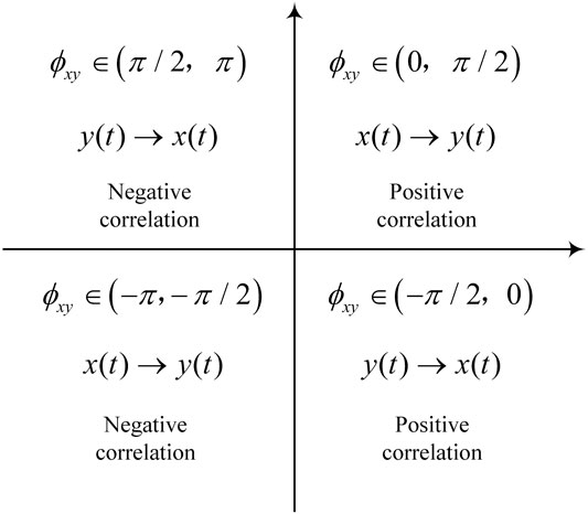
FIGURE 2. Interpretation of phase-difference. Note: the arrow between the variables indicates the direction of causality.

Partial Phase-Difference and Partial Wavelet Gain

Partial phase-difference is introduced to incorporate energy transition and trade openness into the estimation of dynamic causality relationship between economic growth and carbon emission. And partial wavelet gain can be estimated to identify the real effect of economic growth on carbon emission, after controlling for influence from other factors.

The smoothed cross-wavelet transform is denoted as $S_{ij}=S\left(W_{ij}\right)$. We can take these smoothed wavelet transforms as elements to construct a matrix $\mathbb{S}and{\mathbb{S}}_{ij}^d$ denotes the cofactor of the element in position $(i,j)$. The multivariate complex wavelet coherency for $x_1$ and $x_2,\cdots ,x_p$ is given by:

where ${\mathbb{k}}^i=\{\mathrm{1,2},\cdots ,p\}\backslash \left\{i\right\}$.

The complex partial wavelet coherency for $x_1$ and $x_i(2\le i\le p)$ is calculated according to the following equation:

Taking the modulus of complex coherency, the partial wavelet coherency $R_{\left(1,i|{\mathbb{k}}^i\right)}=\text{|}{R}_{\left(1,i|{\mathbb{k}}^i\right)}^c|$ is obtained.

Similar to the definition of the wavelet phase-difference in the case of two variables, we can define the partial wavelet phase-difference between $x_1$ and $x_i(2\le i\le p)$ in the multivariate case after controlling the influence of other variables:

where $\Im ({\rho }_{(1,i|{\mathbb{k}}^i)}^c)$ and $\Re ({\rho }_{(1,i|{\mathbb{k}}^i)}^c)$ represent the imaginary and real parts of the complex wavelet coherency ${\rho }_{(1,i|{\mathbb{k}}^i)}^c$. The cross wavelet gain is defined as follows:

which can be interpreted as the absolute value of regression coefficient in the regression of $y$ on $x$. Taking account of other variables, the formula for the partial wavelet gain is given by

$G_{(1,i|{\mathbb{k}}^i)}$ can be interpreted as the absolute value of coefficients (in modulus) of multivariate regression of $x_1$on $x_2,\mathrm{...},x_p$ at each point of time and frequency. According to Aguiar-Conraria et al. (2018), wavelet gain should be interpreted simultaneously with the phase-difference, which reveals the sign of correlation and the direction of causality.

Data and Empirical Results

Data

The data used in this study are obtained from three sources, including the World Bank WDI database³, the Global Carbon Project⁴, and the BP Statistical Review of World Energy⁵. The definition of variables and data sources are presented in Table 1. The decoupling analysis is based on the level series of emission and GDP, while the wavelet analysis is conducted after taking a first-order difference of these two variables. In the robustness examination, we also take the first-order difference of labor force.

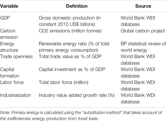
TABLE 1. Data sources and variable definition.

Compared to previous studies, we gather emission and energy structure data from additional sources other than the WDI database to obtain original real GDP and CO2 emission series. Inputs such as capital and labor are also included in the estimation to perform a robustness check for omitted variable. And we use industry value added to proxy the level of economic development. In this way, we are able to alleviate concerns about the impact of economic development on the growth–emission relationship. The descriptive statistics are provided in Table 2. There exists significant heterogeneity in country-specific carbon emission and energy structure among the BRICS countries. It is natural that the relationship between emission and economic growth will vary across these countries.

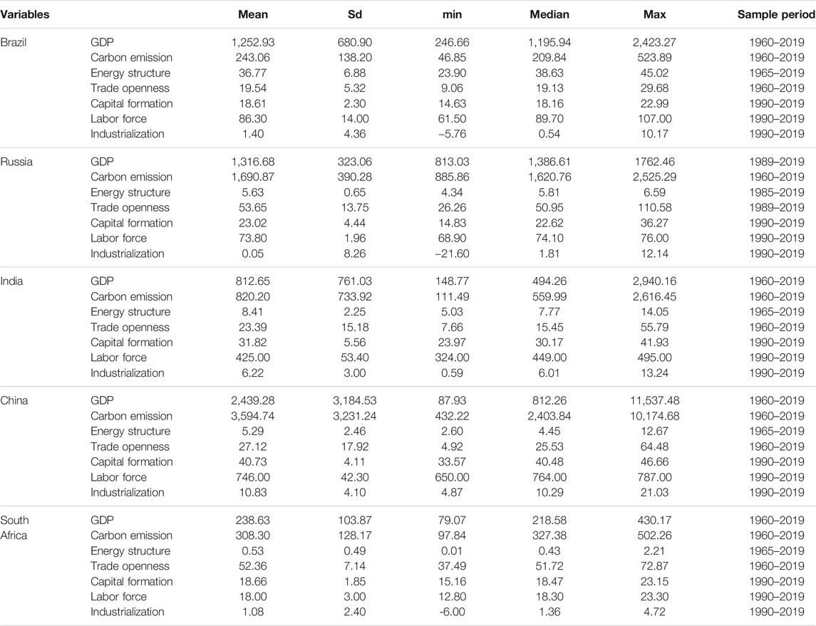
TABLE 2. Descriptive statistics.

Decoupling Analysis

Following the Tapio approach, we calculate the decoupling elastic coefficients between emission and economic growth during the period of 1960–2019 for the BRICS countries, as shown in Table 3. The decoupling states are marked by different colors. As it can be observed, the decoupling indexes of different countries in different periods show great differences.

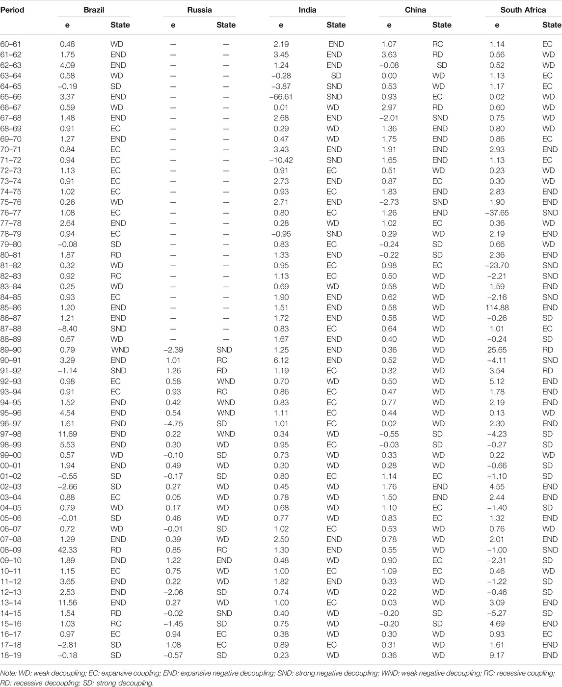
TABLE 3. Decoupling states of carbon emission and economic growth.

In Brazil, the expansive negative decoupling state appears the most frequently during the period of 1960–2019, which demonstrates that the growth rate of carbon emission is higher than that of economic development. The expected strong decoupling state appears during 1964–1965, 1979–1980, 2001–2003, 2005–2006, and 2017–2019, showing that economy grew while carbon emission decreasing at the same time, and the state of strong decoupling and weak decoupling appears more frequently in the period of 2000–2019. Evaluations of the period 2004 to 2009 are compared with the period 1980 to 1994 when Brazil also experienced an apparent decoupling (Freitas and Kaneko, 2011).

For Russia, we focus on analyzing the results after 1989. The strong decoupling state and weak decoupling state are two of the most frequent decoupling states, especially from 1998 to 2019. There also exist recessive coupling in 2008–2009, expansive negative decoupling in 2009–2010, strong negative decoupling in 2014–2015, and expansive coupling in 2016–2018.

The three major types of the decoupling state that appeared in India each account for about 30% of the sample during the whole period: weak decoupling, expansive coupling, and expansive negative decoupling. And we observed that weak decoupling has become a trend since 2000 in India. The expected strong decoupling state appears in 1963–1964, and strong negative decoupling appears in 1964–1966 and 1971–1972.

Weak decoupling state appears the most frequently in China from 1960 to 2019, especially after 1978. This result indicates aggressive efforts in the field of energy conservation and emission reduction made by China. There emerged six different decoupling states during the sample period: recessive coupling in 1960–1961, recessive decoupling in 1961–1962 and 1966–1967, strong decoupling in 1962–1963, weak decoupling in 1963–1965 and 1972–1973, expansive coupling in 1965–1966 and 1973–1974, strong negative decoupling in 1967–1968 and 1975–1976, and expansive negative decoupling in the remaining time period. The expansive coupling state that appeared from 2009 to 2011 may be caused by the recovery after the world economic crisis in 2008.

The results for South Africa are similar to those of Brazil. Expansive negative decoupling state appears the most frequently, which is followed by weak decoupling state and strong decoupling state. It is obvious that the decoupling index of South Africa fluctuates significantly. The expected strong decoupling state appears more frequently after 1997.

In general, the relationship between economic growth and carbon emission is variable and reflects different patterns of economic development. The results from the Tapio decoupling model only provide decoupling state from an elastic perspective in a certain period. In the following section, wavelet transform is introduced to perform an in-depth analysis in the time-frequency domain for richer results.

Wavelet Analysis

The continuous wavelet transform method makes it possible to analyze the complex and evolving impact of economic growth on carbon emission that varies over time and across different frequencies. We estimate partial coherency, partial phase-difference, and partial wavelet gain at different frequencies and over time. Not only the time-varying impact of economic growth on carbon emission, but also the influences from the covariates are well identified. When the partial phase-difference and wavelet gain are estimated regarding a given variable, other variables are served as covariates. The results for each BRICS country are interpreted as follows.

China has been experiencing booming economy and significant shift of growth mode. We analyze the impact of China’s GDP growth on carbon emission in short-, medium-, and long-term horizons. As shown in Figure 3, the partial wavelet coherency between carbon emission and GDP growth suggests more consistent correlation between these two variables in the medium- and long-term. And in the early stage of China’s economic development, partial phase-difference indicator is near zero, indicating non-causality between economic growth and carbon emission.

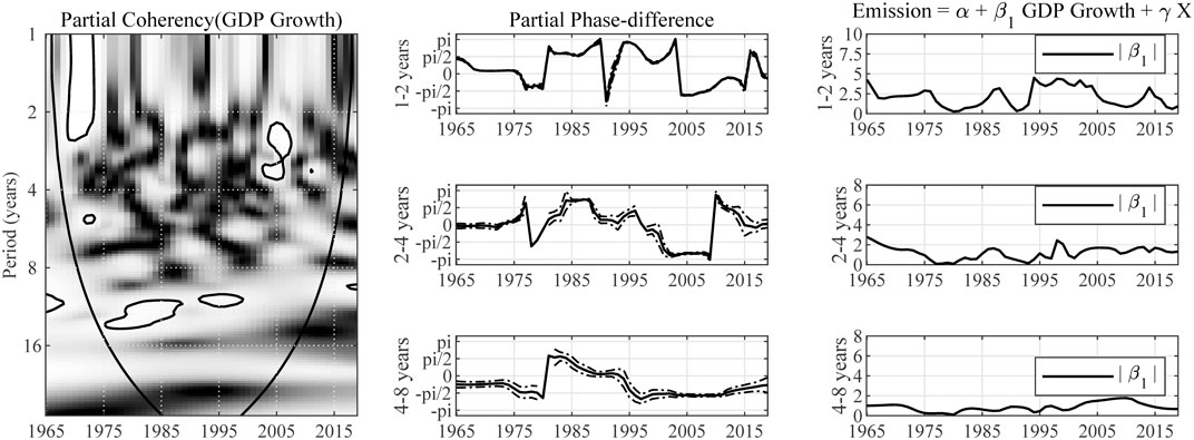
FIGURE 3. Impact of GDP growth on carbon emission in China. Note: The expression “Partial Coherency (GDP Growth)” denotes the partial coherency between GDP growth and carbon emission, controlled for the influence from energy structure and trade openness. The areas below the symmetric black convex curve that appears in the figure of coherency are called the “Cone of Influence (COI),” in which the edge effects are profound. Inside the COI, the results tend to be unreliable. The contours in the coherency diagrams indicate 5% significance level, bootstrapped for 10,000 replications. And, the brighter colors correspond to higher significance level, and darker colors correspond to lower significance level. The dotted lines accompanying the partial phase-difference indicate the 95% confidence intervals.

In the short term (with a period of 1–2 years), relationship between emission and growth is fluid. In the period of 1975–1980, the partial phase-difference is estimated to be between $-\pi /2$ and 0, which indicates that the increase in emission rate leads to GDP growth. In this period, China’s GDP growth depends on heavy industry. The extensive growth mode implies expansion in energy-consuming industries, along with emission surge, will result in higher growth rate. As for 1980–2004, the partial phase-difference is estimated to be between $\pi /2$ and $\pi$ with occasional large deviations around the years around 1991. It indicates negative correlation and causality from emission to GDP growth in general, which suggests that the increasing carbon emission restrains the growth of economy. The reason behind this is that after the rapidly growing phase of the economy development, carbon emission starts to inhibit economic growth to a certain degree; at the same time, the dramatic increase in emission pushes the government to balance the goal of economic expanding and the environment. In the period of 2004–2010, the partial phase-difference is estimated to be between $-\pi$ and $-\pi /2$, which indicates that reduced carbon emission leads to increased GDP growth rate during this period. It is largely the result of the transition of economic growth mode and the enhanced awareness of environmental protection. For the time after 2010, the results are quite mixed, reflecting impact of cross currents in the economy after the shock of the financial crisis.

In the medium-term (with a period of 2–4 years), it can be observed that the pattern of variation in partial phase-difference and wavelet gain is very similar to that in the short-term. So, more attention is paid to the results from the perspective of long-term.

In the long run (with a period of 4–8 years), the partial wavelet gain of carbon emission over GDP growth is around 1. It is smaller than that in the short- and medium-term due to the fact that influences from temporary factors fade out eventually. During the period of 1970–1979, the partial phase-difference is estimated to be between $-\pi /2$ and 0, which indicates that the increase in emission rate poses positive impact on GDP growth rate. From 1980 to 1994, the partial phase-difference is estimated to be between 0 and $\pi /2$, suggesting that increase in GDP growth rate causes higher carbon emission. During this period, China was experiencing an unprecedented rapid economic growth, and the environmental consideration did not feature prominently in the government's policy goals yet. The partial phase-difference lies in the interval $\left(-\pi ,-\pi /2\right)$ from 1995 to 2013, which means with the increasing of GDP growth, the growth rate of carbon emissions decreased. The significant decoupling of emission from economic growth attributes to the effective environmental protection measures and the promoting usage of renewable energy in China.

The partial wavelet coherency between energy structure and carbon emission in China indicates that there is a significant correlation between proportion of renewable energy consumption and carbon emissions (see Figure 4). And the partial wavelet gain results show a decreasing trend of marginal impact of energy structure on carbon emission throughout the sample period, regardless of the perspectives of time-spans.

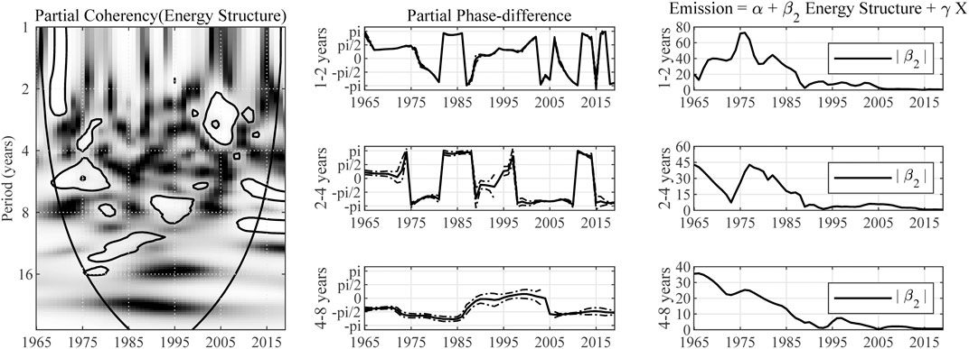
FIGURE 4. Impact of energy structure on carbon emission in China. Note: The expression “Partial Coherency (Energy Structure)” denotes the partial coherency between energy structure and carbon emission, controlled for the influence from economic growth and trade openness. The areas below the symmetric black convex curve that appears in the figure of coherency are called the “Cone of Influence (COI),” in which the edge effects are profound. Inside the COI, the results tend to be unreliable. The contours in the coherency diagrams indicate 5% significance level, bootstrapped for 10,000 replications. And, the brighter colors correspond to higher significance level, and darker colors correspond to lower significance level. The dotted lines accompanying the partial phase-difference indicate the 95% confidence intervals.

In the short-term and medium-term, the partial phase-difference falls into the range of $\left(0,\pi /2\right)$ from 1967 to 1975, indicating that the increase in renewable energy share is accompanied by higher level of carbon emission. The main reason behind this unusual result is that China was hungered for energy from all sources to support its economic development during this period. In the following period of 1975 to 1980, the partial phase-difference falls into the interval of $\left(-\pi ,-\pi /2\right)$, showing that the increasing proportion of renewable energy leads to lowering the growth rate of emission. From 1981 to 1986, the partial phase-difference falls into the range of $\left(\pi /2,\pi \right)$. This means that the increasing emission is a cause of higher proportion of renewable energy consumption, which implies that economic growth has once again become the country’s top priority. In the following sample period, the partial phase-difference fluctuates across all four quadrants frequently, reflecting ambiguous causality relationship.

The results from the perspective of medium-term are similar to those in the short-term, except for the sharp dive of partial phase-difference in 1996. This sudden drop may reflect the impact of changes in national policy which emphasizes the importance of development of new and renewable energy⁶.

In the long-term, the partial phase-difference is estimated to fall into the range of $\left(-\pi ,-\pi /2\right)$ from 1970 to 1987, suggesting an emission reduction effect of increasing share of renewable energy consumption. From 1990 to 2004, the partial phase-difference falls into the interval of $\left(0,\pi /2\right)$. After the reform and opening up, China’s economic growth was largely driven by the introduction of energy-inefficient technologies, which had depressed the carbon reduction effect of renewable energy consumption. From 2005 to 2013, the partial phase-difference falls into the range of $\left(-\pi ,-\pi /2\right)$, indicating that production energy efficiency has begun to improve and a greater proportion of renewable energy has been a significant cause of the decline in the growth rate of carbon emissions.

According to the wavelet coherency estimates in Figure 5, there exists significant and consistent correlation between emission and trade openness. In the short-term, the partial phase-difference lies in $\left(-\pi /\mathrm{2,0}\right)$ from 1967 to 1994 and the period of 2004–2015, indicating positive impact of carbon emission on trade openness. That is because China was a major producer of industrial semifinished products in the period from 1967 to 1994. The export of these products has resulted in a significant increase in China’s trade volume, such that China’s increasing carbon emission rate was followed by higher proportion of trade to GDP. And this effect was evident again after China’s entry into the World Trade Organization. The result for the period from 1994 to 2004 shows the positive impact of trade openness on the emission rate. In the long run, the partial phase-difference lies in $\left(-\pi /\mathrm{2,0}\right)$ and $\left(0,\pi /2\right)$ respectively during the periods 1972–1994 and 1994–2013. The relationship between trade openness and carbon emission is quite consistent with the results in the short-term.

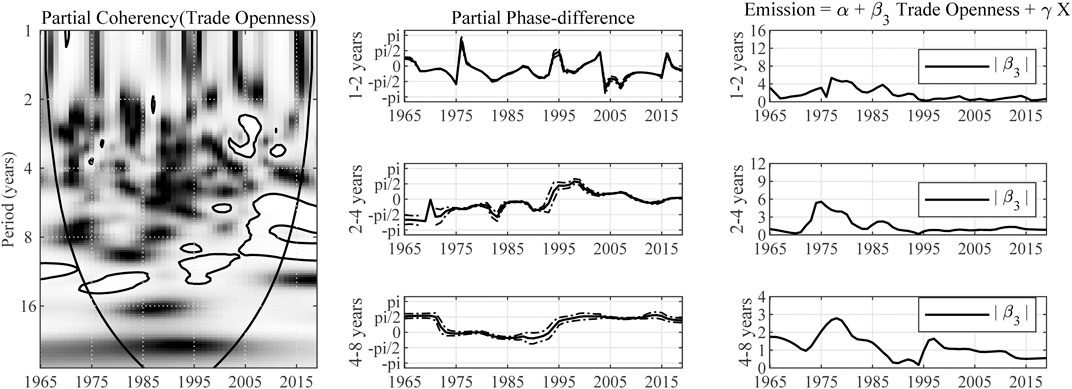
FIGURE 5. Impact of trade openness on carbon emission in China. Note: The expression “Partial Coherency (Trade Openness)” denotes the partial coherency between trade openness and carbon emission, controlled for the influence from energy structure and economic growth. The areas below the symmetric black convex curve that appears in the figure of coherency are called the “Cone of Influence (COI),” in which the edge effects are profound. Inside the COI, the results tend to be unreliable. The contours in the coherency diagrams indicate 5% significance level, bootstrapped for 10,000 replications. And, the brighter colors correspond to higher significance level, and darker colors correspond to lower significance level. The dotted lines accompanying the partial phase-difference indicate the 95% confidence intervals.

The results of multivariate wavelet analysis for Russian are presented in Figure 6. According to partial coherency between GDP growth and emission, the correlation is much more significant in the short-term. This result implies a temporary relationship between these two variables. The estimated partial wavelet gain of emission over GDP growth is approximately 0.5, which is quite constant across different frequencies.

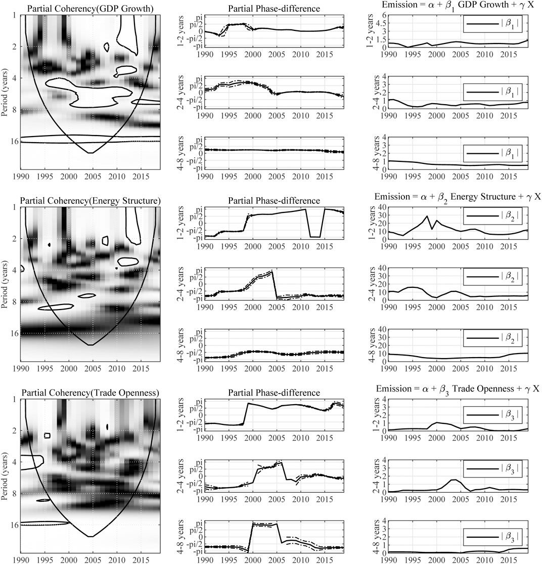
FIGURE 6. Multivariate wavelet analysis results for Russia. Note: The expression “Partial Coherency (Z)” denotes the partial coherency between variable Z and carbon emission, controlled for the influence from other factors. The areas below the symmetric black convex curve that appears in the figure of coherency are called the “Cone of Influence (COI),” in which the edge effects are profound. Inside the COI, the results tend to be unreliable. The contours in the coherency diagrams indicate 5% significance level, bootstrapped for 10,000 replications. And, the brighter colors correspond to higher significance level, and darker colors correspond to lower significance level. The dotted lines accompanying the partial phase-difference indicate the 95% confidence intervals.

In the short-term, the partial phase-difference lies in $\left(-\pi /\mathrm{2,0}\right)$ from 1992 to 1994, indicating that the increasing of emission rate causes higher rate of GDP growth. From 1994 to 2018, the partial phase-difference is greater than 0 and less than $\pi /2$ all along. As a typical industrial economy, the Russian production system is dominated by heavy industries, resulting in the causality from GDP growth to higher level of carbon emission. In the long run, the partial phase-difference falls into the range of $\left(0,\pi /2\right)$ throughout the whole sample period. This result reveals the dependence of Russia's economic growth on high-emission heavy industry in the long-term and the persistent impact of growth on emission.

As for other factors, the partial phase-difference between emission and energy structure is estimated to be between $-\pi$ and $-\pi /2$ in the long-term. And the partial wavelet gain is estimated to be approximately 10. These results indicate that the rising proportion of renewable energy has effectively restrained the growth of carbon emission rate since the 1990s. The partial wavelet gain of emission over trade openness is approximately 0.2 in the long-term, implying a much weaker impact on carbon emission other than energy structure. And the partial coherency also provides evidence of insignificant correlation between trade openness and carbon emission.

In Figure 7 we observe a significant correlation between Brazil’s economic growth and carbon emission. The partial wavelet gain of emission over GDP growth is approximately 1. In both short-term and long-term, the partial phase-difference roughly falls into the range of $\left(-\pi ,-\pi /2\right)$ from 1996 to 2004, reflecting the inhibitory effect of the increase of GDP growth rate on the growth rate of carbon emissions. Brazil currently possesses one of the most sustainable energy structures among the emerging economies. There is 44.1% of energy supply coming from renewable sources, and approximately 81.7% of all electricity supply coming from hydropower (Hsiao-Tien and Hsin-Chia, 2013).

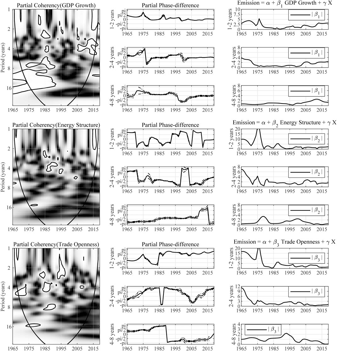
FIGURE 7. Multivariate wavelet analysis results for Brazil. Note: The expression “Partial Coherency (Z)” denotes the partial coherency between variable Z and carbon emission, controlled for the influence from other factors. The areas below the symmetric black convex curve that appears in the figure of coherency are called the “Cone of Influence (COI),” in which the edge effects are profound. Inside the COI, the results tend to be unreliable. The contours in the coherency diagrams indicate 5% significance level, bootstrapped for 10,000 replications. And, the brighter colors correspond to higher significance level, and darker colors correspond to lower significance level. The dotted lines accompanying the partial phase-difference indicate the 95% confidence intervals.

As for other factors, the partial coherency between energy structure and carbon emission seems insignificant in most areas. And the long-term partial phase-difference between emission and trade openness falls into the range of $\left(\pi /2,\pi \right)$ from 1972 to 1989, and into the range of $\left(-\pi ,-\pi /2\right)$ from 1990 to 2015. When the correlation remains negative, the leading variable has changed from carbon emissions to trade openness after 1990, indicating a reversion in the direction of causality. The relationship between the two variables has shifted from that carbon emission restricts scale of international trade to that increased trade openness mitigating the growth of carbon emission.

A careful look at India's NDC reveals that India’s climate commitment is grounded on various macroeconomic indicators such as GDP growth, emission intensity, mix of energy sources, and changing structure of the economy, which are also drivers of carbon emission (Nandini and Joyashree, 2020). As presented in Figure 8, the partial wavelet gain of emission over GDP growth is approximately 1 and the partial coherency indicates a significant correlation between the two variables only in a small area. Compared with countries previously discussed, the correlation between India’s economic growth and carbon emissions is relatively weak. The long-run partial phase-difference falls into the range of $\left(-\pi /2,\pi /2\right)$ from 1965 to 2015, and implies a positive correlation between the two variables in the long-term. But, the low significant level of partial coherency makes it meaningless for the correlation and causality inference. As for the energy structure and trade openness, estimated partial coherency suggests low significant level of correlation and causality.

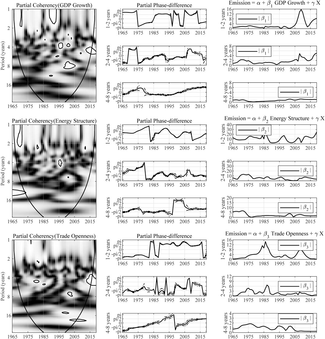
FIGURE 8. Multivariate wavelet analysis results for India. Note: The expression “Partial Coherency (Z)” denotes the partial coherency between variable Z and carbon emission, controlled for the influence from other factors. The areas below the symmetric black convex curve that appears in the figure of coherency are called the “Cone of Influence (COI),” in which the edge effects are profound. Inside the COI, the results tend to be unreliable. The contours in the coherency diagrams indicate 5% significance level, bootstrapped for 10,000 replications. And, the brighter colors correspond to higher significance level, and darker colors correspond to lower significance level. The dotted lines accompanying the partial phase-difference indicate the 95% confidence intervals.

South Africa is one of the world’s most carbon-intensive economies (Marcel, 2013). As presented in Figure 9, partial phase-difference is estimated to be between $-\pi /2$ and $\pi /2$ during 1976–2015. It is easy to observe that there is a strong positive correlation between the emission and GDP growth in the long run. Given that most of South Africa's energy needs are met by fossil fuels, and considering its status as a non-oil producer, a strong link between energy structure and CO2 emissions is to be expected. The partial phase-difference is estimated to be between $\pi /2$ and $\pi$ and between $-\pi$ and $-\pi /2$ in the most time, indicating a strong negative correlation in the long run. The result also suggests causality from increase in GDP growth to slower adoption of renewable energy, before 1990. And the improving energy structure starts to mitigate incremental carbon emission ever since 1996.

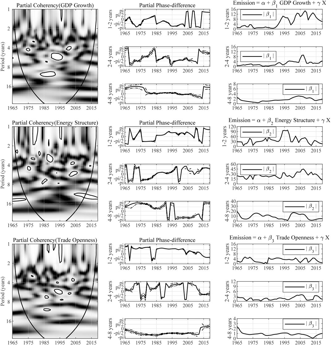
FIGURE 9. Multivariate wavelet analysis results for South Africa. Note: The expression “Partial Coherency (Z)” denotes the partial coherency between variable Z and carbon emission, controlled for the influence from other factors. The areas below the symmetric black convex curve that appears in the figure of coherency are called the “Cone of Influence (COI),” in which the edge effects are profound. Inside the COI, the results tend to be unreliable. The contours in the coherency diagrams indicate 5% significance level, bootstrapped for 10,000 replications. And, the brighter colors correspond to higher significance level, and darker colors correspond to lower significance level. The dotted lines accompanying the partial phase-difference indicate the 95% confidence intervals.

Robustness

There is little consensus on that the causality relationship has been reached in the field of the energy consumption–economic growth nexus due to the omitted variable bias. So, we have reasons to concern that our empirical results also suffer from the omitted variable problem. We follow the approach from prior researches to examine whether the empirical results suffer from this problem (see Lean and Smyth, 2010; Apergis and Payne, 2010a; Apergis and Payne, 2010b; Apergis and Payne, 2011a; Apergis and Payne, 2011b). The physical inputs and a proxy of economic development are introduced and the multivariate wavelet analysis is conducted as a robustness check. The multivariate wavelet analysis results with these additional control variables are presented in Figure 10.

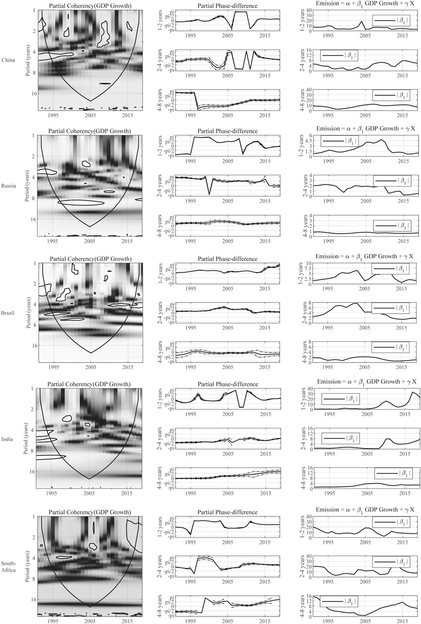
FIGURE 10. Multivariate wavelet analysis results controlled for additional factors. Note: The expression “Partial Coherency (Z)” denotes the partial coherency between variable Z and carbon emission, controlled for the influence from other factors. The areas below the symmetric black convex curve that appears in the figure of coherency are called the “Cone of Influence (COI),” in which the edge effects are profound. Inside the COI, the results tend to be unreliable. The contours in the coherency diagrams indicate 5% significance level, bootstrapped for 10,000 replications. And, the brighter colors correspond to higher significance level, and darker colors correspond to lower significance level. The dotted lines accompanying the partial phase-difference indicate the 95% confidence intervals.

As Figure 10 demonstrates, the results are consistent with those reported in previous sections, with certain difference in statistic values. The reason may be the shortened sample period due to the inclusion of more variables. We believe the adoption of wavelet analysis not only makes it possible to extract more abundant information from the perspective of time and frequency, but also alleviates the interference caused by omitted variable problem to a certain extent.

Conclusion

The decoupling relationship between economic growth and carbon emissions has received extensive academic discussion. But the dynamic time-varying impact of growth on carbon emission has not received enough attention. Besides the decoupling analysis, this paper further introduces the wavelet analysis method that estimates the dynamic relationship in time-frequency space to fill this gap.

The results of the decoupling analysis show that only China exhibits an obvious decoupling trend among the BRICS countries. This result indicates aggressive efforts in the field of energy conservation and emission reduction made by China. The decoupling indies of other four emerging economies are relatively mixed, and part of them are more of an irregular list of decoupling states at different time points.

The wavelet analysis provides more extensive results, fully considering the influence of covariates and the time-varying characteristics of the relationship between variables. Among the BRICS countries, coherency analysis indicates a significant impact of economic growth on carbon emission only in China, Russia, and Brazil.

In the early stage of China’s economic development, the near-zero partial phase-difference indicates a non-causality relationship between the economic growth and carbon emission. When the expansion of heavy industries gets started, the accompanying emission leads to rise in the growth rate. And after the country enters a path of rapid growth, the increase in growth rate continues to push up carbon emission. Until 1995, the economic growth starts to suppress carbon emission growth. This is largely the result of transition of economic growth mode, change in energy structure, and enhanced awareness of environmental protection. Trade openness generally has a positive impact on emission, due to China’s long-standing trade surplus.

Results from wavelet analysis reveal the dependence of Russia's economic growth on high-emission heavy industry in the long-term and the persistent positive causality from economic growth to carbon emission. Meanwhile, the improvement of energy structure helps in effectively restraining the growing carbon emission ever since the 1990s. And there is no obvious evidence that trade openness has a certain effect on carbon emission.

Estimation based on data from Brazil implies a significant inhibitory effect of the increase of GDP growth rate on the rise of carbon emissions. It attributes to the abundant renewable energy resources such that improvement in energy structure does not play a significant role in reducing emission. And increased openness helps in mitigating the growth of carbon emissions in Brazil since 1990.

In conclusion, different resource endowments and growth patterns lead to different impacts of economic growth on carbon emissions and the time-varying characteristics of the causality relationship between them. In addition to economic growth, changes in a country's energy structure and trade openness can also significantly affect carbon emissions. When the government formulates relevant carbon emission targets and emission reduction policies, it is necessary to pay full attention to the dynamic impact of economic growth, energy structure, and trade openness to carbon emission.

Data Availability Statement

The original contributions presented in the study are included in the article/Supplementary Material, further inquiries can be directed to the corresponding author.

Author Contributions

LX: software, validation, resources, data curation, writing original draft. XC: writing—review and editing, and visualization. SS: conceptualization, methodology, formal analysis, investigation. ZY: writing—review and editing, supervision, project administration, and funding acquisition. All authors: contributed to the article and approved the submitted version.

Conflict of Interest

The authors declare that the research was conducted in the absence of any commercial or financial relationships that could be construed as a potential conflict of interest.

Publisher’s Note

All claims expressed in this article are solely those of the authors and do not necessarily represent those of their affiliated organizations, or those of the publisher, the editors and the reviewers. Any product that may be evaluated in this article, or claim that may be made by its manufacturer, is not guaranteed or endorsed by the publisher.

Acknowledgments

We show our gratitude to participants at the Taishan Financial Forum for their helpful comments. We acknowledge the financial support from Shandong Provincial Natural Science Foundation (Grant Number: ZR2020QG032), Shandong Provincial Social Science Planning Office (Grant Numbers: 21DGLJ12; 21DJJJ02), Taishan Scholars Program of Shandong Province, China (Grant Numbers: ts201712059; tsqn201909135) and Youth Innovative Talent Technology Program of Shandong Province, China (Grant Number: 2019RWE004). All errors remain our own.

Footnotes

¹https://www.iea.org/cetp/.

²Clean Energy Transitions Program (CETP) Annual Report 2018.

³World Development Indicators (WDI) database from World Bank, available at: http://wdi.worldbank.org.

⁴Global Carbon Project. (2020). Supplemental data of Global Carbon Budget 2020 (Version 1.0) (Data set). Available at: https://doi.org/10.18160/gcp-2020.

⁵BP Statistical Review of World Energy. Available at: http://www.bp.com/statisticalreview.

⁶New and renewable energy development plan: 1996–2010, issued in 1995.

References

Adedoyin, F. F., Gumede, M. I., and Bekun, F. V. (2020). Modelling Coal Rent, Economic Growth and CO2 Emissions: Does Regulatory Quality Matter in BRICS Economies?. Sci. Total Environ. 710, 136284. doi:10.1016/j.scitotenv.2019.136284
Aguiar-Conraria, L., Martins, M. M. F., and Joana Soares, M. (2018). Estimating the Taylor Rule in the Time-Frequency Domain. J. Macroeconomics 57, 122–137. doi:10.1016/j.jmacro.2018.05.008
Antweiler, W., Copeland, R. B., and Taylor, M. S. (2001). Is Free Trade Good for the Environment?. Am. Econ. Rev. 80, 15–27. doi:10.1257/aer.91.4.87
Apergis, N., Christou, C., and Gupta, R. (2017). Are There Environmental Kuznets Curves for US State Level CO2 Emissions?. Renew. Sustain. Energ. Rev. 69, 551–558. doi:10.1016/j.rser.2016.11.219
Apergis, N. (2016). Environmental Kuznets Curves: New Evidence on Both Panel and Country-Level CO2 Emissions. Energ. Econ. 54, 263–271. doi:10.1016/j.eneco.2015.12.007
Apergis, N., Payne, J. E., Menyah, K., and Wolde-Rufael, Y. (2010). On the Causal Dynamics between Emissions, Nuclear Energy, Renewable Energy, and Economic Growth. Ecol. Econ. 69 (11), 2255–2260. doi:10.1016/j.ecolecon.2010.06.014
Apergis, N., and Payne, J. E. (2011a). Renewable and Non-renewable Electricity Consumption Growth Nexus: Evidence from Emerging Market Economies. Appl. Energ. 88 (12), 5226–5230. doi:10.1016/j.apenergy.2011.06.041
Apergis, N., and Payne, J. E. (2012). Renewable and Non-renewable Energy Consumption-Growth Nexus: Evidence from a Panel Error Correction Model. Energ. Econ. 34 (3), 733–738. doi:10.1016/j.eneco.2011.04.007
Apergis, N., and Payne, J. E. (2010a). Renewable Energy Consumption and Growth in Eurasia. Energy Economics 32 (6), 1392–1397. doi:10.1016/j.eneco.2010.06.001
Apergis, N., and Payne, J. E. (2011b). The Renewable Energy Consumption–Growth Nexus in Central America. Appl. Energ. 88 (1), 343–347. doi:10.1016/j.apenergy.2010.07.013
Apergis, N., and Payne, J. E. (2010b). The Emissions, Energy Consumption, and Growth Nexus: Evidence from the Commonwealth of Independent States. Energy Policy 38 (1), 650–655. doi:10.1016/j.enpol.2009.08.029
Apergis, N., and Tang, C. F. (2013). Is the Energy-Led Growth Hypothesis Valid? New Evidence from a Sample of 85 Countries. Energ. Econ. 38, 24–31. doi:10.1016/j.eneco.2013.02.007
Baek, J., Cho, Y., and Koo, W. W. (2009). The Environmental Consequences of Globalization: a Country-specific Time-Series Analysis. Ecol. Econ. 68, 2255–2264. doi:10.1016/j.ecolecon.2009.02.021
Banerjee, S., and Murshed, M. (2020). Do emissions Implied in Net export Validate the Pollution haven Conjecture? Analysis of G7 and BRICS Countries. Int. J. Sustain. Economy. 12, 297. doi:10.1504/IJSE.2020.111539
Bloomfield, D., McAteer, R., Lites, B., Judge, P., Mathioudakis, M., and Keena, F. (2004). Wavelet Phase Coherence Analysis: Application to a Quiet-Sun Magnetic Element. Astrophysical J. 617, 623–632. Available at: https://iopscience.iop.org/article/10.1086/425300. doi:10.1086/425300
Climent, F., and Pardo, A. (2007). Decoupling Factors on the Energy-Output Linkage: the Spanish Case. Energy Pol 35, 522–528. doi:10.1016/j.enpol.2005.12.022
Cole, M. A., and Elliott, R. J. (2003). Determining the Trade–Environment Composition Effect: the Role of Capital, Labor and Environmental Regulations. J. Environ. Econ. Manage. 46 (3), 363–383. doi:10.1016/S0095-0696(03)00021-4
Copeland, B., and Taylor, M. S. (2003). Trade and the Environment: Theory and Evidence. Princeton, NJ: Princeton University Press. Available at: http://refhub.elsevier.com/S0140-9883(20)30306-6/rf0110.
Csereklyei, Z., and Stern, D. I. (2015). Global Energy Use: Decoupling or Convergence?. Energ. Econ. 51, 633–641. doi:10.1016/j.eneco.2015.08.029
Dai, S., Zhang, M., and Huang, W. (2016). Decomposing the Decoupling of CO2 Emission from Economic Growth in BRICS Countries. Nat. Hazards 84 (2), 1055–1073. doi:10.1007/s11069-016-2472-0
Dauda, L., Xingle, L., Mensah, C. N., Salman, M., Boamah, K. B., Ampon-Wireko, S., et al. (2021). Innovation, Trade Openness and CO2 Emissions in Selected Countries in Africa. J. Clean. Prod. 281, 125143. doi:10.1016/j.jclepro.2020.125143
Dong, B., Zhang, M., Mu, H. L., and Su, X. M. (2016). Study on Decoupling Analysis between Energy Consumption and Economic Growth in Liaoning Province. Energ. Pol 97, 414–420. doi:10.1016/j.enpol.2016.07.054
Dong, B., Ma, X., Zhang, Z., Zhang, H., Chen, R., Song, Y., et al. (2020). Carbon Emissions, the Industrial Structure and Economic Growth: Evidence from Heterogeneous Industries in China. Environ. Pollut. 262, 114322. doi:10.1016/j.envpol.2020.114322
Dottori, F., Szewczyk, W., Ciscar, J.-C., Zhao, F., Alfieri, L., Hirabayashi, Y., et al. (2018). Increased Human and Economic Losses from River Flooding with Anthropogenic Warming. Nat. Clim. Change 8 (9), 781–786. doi:10.1038/s41558-018-0257-z
Enevoldsen, M. K., Ryelund, A. V., and Andersen, M. S. (2007). Decoupling of Industrial Energy Consumption and CO2-emissions in Energy-Intensive Industries in Scandinavia. Energy Econ 29, 665–692. doi:10.1016/j.eneco.2007.01.016
Fragkos, P., Laura van Soest, H., Schaeffer, R., Reedman, L., Koberle, A. C., Macaluso, N., et al. (2021). Energy System Transitions and Low-Carbon Pathways in Australia, Brazil, Canada, China, EU-28, India, Indonesia, Japan, Republic of Korea, Russia and the United States. Energy 216, 119385. doi:10.1016/j.energy.2020.119385
Frankel, J., and Rose, A. (2005). Is Trade Good or Bad for the Environment? Sorting Out the Causality. Rev. Econ. Stat. 87 (1), 85–91. doi:10.1162/0034653053327577
Freitas, L. C., and Kaneko, S. (2011). Decomposing the Decoupling of CO2 Emissions and Economic Growth in Brazil. Ecol. Econ. 70, 1459–1469. doi:10.1016/j.ecolecon.2011.02.011
Galeotti, M., Manera, M., and Lanza, A. (2009). On the Robustness of Robustness Checks of the Environmental Kuznets Curve Hypothesis. Environ. Resource Econ. 42 (4), 551–574. doi:10.1007/s10640-008-9224-x
Gan, P. Y., and Li, Z. D. (2008). An Econometric Study on Long-Term Energy Outlook and the Implications of Renewable Energy Utilization in Malaysia. Energy Policy 2, 890–899. doi:10.1016/j.enpol.2007.11.003
Gao, D., Zhou, H., Wang, J., Miao, S., Yang, F., Wang, G., et al. (2015). Size-Dependent Electrocatalytic Reduction of CO2 over Pd Nanoparticles. J. Am. Chem. Soc. 137 (13), 4288–4291. doi:10.1021/jacs.5b00046
Grinsted, A., Moore, J. C., and Jevrejeva, S. (2004). Application of the Cross Wavelet Transform and Wavelet Coherence to Geophysical Time Series. Nonlinear Process. Geophys. 11, 561–566. doi:10.5194/npg-11-561-2004
Grossman, G., and Krueger, A. (1991). Environmental Impacts of the North American Free Trade Agreement. NBER Working Paper. 3914. doi:10.3386/w3914
Guan, D., Meng, J., Reiner, D. M., Zhang, N., Shan, Y., Mi, Z., et al. (2018). Structural Decline in China’s CO2 Emissions through Transitions in Industry and Energy Systems. Nat. Geosci. 11, 551–555. doi:10.1038/s41561-018-0161-1
Hsiao-Tien, P., and Hsin-Chia, F. (2013). Renewable Energy, Non-renewable Energy and Economic Growth in Brazil. Renew. Sustain. Energ. Rev. 25, 381–392. doi:10.1016/j.rser.2013.05.004
Hu, H., Xie, N., Fang, D., and Zhang, X. (2018). The Role of Renewable Energy Consumption and Commercial Services Trade in Carbon Dioxide Reduction: Evidence from 25 Developing Countries. Appl. Energ. 211, 1229–2124. doi:10.1016/j.apenergy.2017.12.019
Hu, M., Li, R., You, W., Liu, Y., and Lee, C. (2020). Spatiotemporal Evolution of Decoupling and Driving Forces of CO2 Emissions on Economic Growth along the Belt and Road. J. Clean. Prod. 277, 123272. doi:10.1016/j.jclepro.2020.123272
Kan, S., Chen, B., and Chen, G. (2019). Worldwide Energy Use across Global Supply Chains: Decoupled from Economic Growth?. Appl. Energ. 250, 1235–1245. doi:10.1016/j.apenergy.2019.05.104
Kovanda, J., and Hak, T. (2007). What Are the Possibilities for Graphical Presentation of Decoupling? an Example of Economy-wide Material Flow Indicators in the Czech Republic. Ecol. Indicators 7, 123–132. doi:10.1016/j.ecolind.2005.11.002
Lean, H. H., and Smyth, R. (2010). CO2 Emissions, Electricity Consumption and Output in ASEAN. Appl. Energ. 87 (6), 1858–1864. doi:10.1016/j.apenergy.2010.02.003
Liu, X., Zhang, S., and Bae, J. (2017). The Nexus of Renewable Energy-Agriculture-Environment in BRICS. Appl. Energ. 204, 489–496. doi:10.1016/j.apenergy.2017.07.077
Loh, L. (2013). Co-movement of Asia–Pacific with European and US Stock Market Returns: a Cross-Time-Frequency Analysis. Res. Int. Business Finance 29, 1–13. doi:10.1016/j.ribaf.2013.01.001
Loo, B. P. Y., and Banister, D. (2016). Decoupling Transport from Economic Growth: Extending the Debate to Include Environmental and Social Externalities. J. Transport Geogr. 57, 134–144. doi:10.1016/j.jtrangeo.2016.10.006
Ma, Q., Murshed, M., and Khan, Z. (2021). The Nexuses between Energy Investments, Technological Innovations, Emission Taxes, and Carbon Emissions in China. Energy Policy 155, 112345. doi:10.1016/j.enpol.2021.112345
Ma, X., Ye, Y., Shi, X., and Zou, L. (2016). Decoupling Economic Growth from CO2 Emissions: a Decomposition Analysis of China’s Household Energy Consumption. Adv. Clim. Change Res. 7, 192–200. doi:10.1016/j.accre.2016.09.004
Managi, S., Hibiki, A., and Tsurumi, T. (2008). Does Trade Liberalization Reduce Pollution Emissions. Discussion papers, 8013. Available at: https://EconPapers.repec.org/RePEc:eti:dpaper:08013 (Accessed May 17, 2021).
Mandler, M., and Scharnagl, M. (2014). Money Growth and Consumer price Inflation in the Euro Area: A Wavelet Analysis. No 33/2014. Berlin: Deutsche Bundesbank. Available at: http://www.bundesbank.de (Accessed May 17, 2021).
Marcel, K. (2013). CO2 Emissions, Energy Consumption, Income and Foreign Trade: A South African Perspective. Energy Policy 63, 1042–1050. doi:10.1016/j.enpol.2013.09.022
Mielnik, O., and Goldemberg, J. (2002). Foreign Direct Investment and Decoupling between Energy and Gross Domestic Product in Developing Countries. Energ. Pol 30, 87–89. doi:10.1016/S0301-4215(01)00080-5
Murshed, M., Alam, R., and Ansarin, A. (2021a). The Environmental Kuznets Curve Hypothesis for Bangladesh: the Importance of Natural Gas, Liquefied Petroleum Gas, and Hydropower Consumption. Environ. Sci. Pollut. Res. 28, 17208–17227. doi:10.1007/s11356-020-11976-6
Murshed, M., Ali, S. R., and Banerjee, S. (2021b). Consumption of Liquefied Petroleum Gas and the EKC Hypothesis in South Asia: Evidence from Cross-Sectionally Dependent Heterogeneous Panel Data with Structural Breaks. Energ. Ecol. Environ. 6, 353. doi:10.1007/s40974-020-00185-z
Murshed, M. (2020). An Empirical Analysis of the Non-linear Impacts of ICTTrade Openness on Renewable Energy Transition, Energy Efficiency, Clean Cooking Fuel Access and Environmental Sustainability in South Asia. Environ. Sci. Pollut. Res. 27, 36254. doi:10.1007/s11356-020-09497-3
Nandini, D., and Joyashree, R. (2020). India Can Increase its Mitigation Ambition: An Analysis Based on Historical Evidence of Decoupling between Emission and Economic Growth. Energ. Sustain. Develop. 57, 189–199. doi:10.1016/j.esd.2020.06.003
Narayan, P. K., and Smyth, R. (2007). A Panel Cointegration Analysis of the Demand for Oil in the Middle East. Energy Policy 35, 6258–6265. doi:10.1016/j.enpol.2007.07.011
Narayan, P. K., Smyth, R., and Prasad, A. (2007). Electricity Consumption in G7 Countries: A Panel Cointegrating Analysis of Residential Demand Elasticities. Energy Policy 35, 4485–4494. doi:10.1016/j.enpol.2007.03.018
Narayan, S. (2016). Predictability within the Energy Consumption-Economic Growth Nexus: Some Evidence from Income and Regional Groups. Econ. Model. 54, 515–521. doi:10.1016/j.econmod.2015.12.037
Obama, B. (2017). The Irreversible Momentum of Clean Energy. Science 355 (6321), 126. doi:10.1126/science.aam6284
Pinsky, M. L., Eikeset, A. M., McCauley, D. J., Payne, J. L., and Sunday, J. M. (2019). Greater Vulnerability to Warming of marine versus Terrestrial Ectotherms. Nature 569 (7754), 108e111. doi:10.5281/zenodo.257619710.1038/s41586-019-1132-4
Rehman, A., Ulucak, R., Murshed, M., Ma, H., and Işık, C. (2021). Carbonization and Atmospheric Pollution in China: The Asymmetric Impacts of Forests, Livestock Production, and Economic Progress on CO2 Emissions. J. Environ. Manage. 294, 113059. doi:10.1016/j.jenvman.2021.113059
Roman-Collado, R., Cansino, J. M., and Botia, C. (2018). How Far Is Colombia from Decoupling? Two-Level Decomposition Analysis of Energy Consumption Changes. Energy 148, 687–700. doi:10.1016/j.energy.2018.01.141
Saboori, B., Sulaiman, J., and Mohd, S. (2012). Economic Growth and CO2 Emissions in Malaysia: a Cointegration Analysis of the Environmental Kuznets Curve. Energy Policy 51, 184–191. doi:10.1016/j.enpol.2012.08.065
Salman, M., Long, X., Dauda, L., Mensah, C. N., and Muhammad, S. (2019). Different Impacts of export and Import on Carbon Emissions across 7 ASEAN Countries: A Panel Quantile Regression Approach. Sci. Total Environ. 686, 1019–1029. doi:10.1016/j.scitotenv.2019.06.019
Selden, T. M., and Song, D. (1994). Environmental Quality and Development: Is There a Kuznets Curve for Air Pollution Emissions?. J. Environ. Econ. Manage. 27 (2), 147–162. doi:10.1006/jeem.1994.1031
Sorrell, S., Lehtonen, M., Stapleton, L., Pujol, J., and Champion, T. (2012). Decoupling of Road Freight Energy Use from Economic Growth in the United Kingdom. Energ. Pol 41, 84–97. doi:10.1016/j.enpol.2010.07.007
Tapio, P. (2005). Towards a Theory of Decoupling: Degrees of Decoupling in the Eu and the Case of Road Traffic in Finland between 1970 and 2001. Transport Pol. 12, 137–151. doi:10.1016/j.tranpol.2005.01.001
Tiba, S., and Frikha, M. (2018). Income, Trade Openness and Energy Interactions: Evidence from Simultaneous Equation Modeling. Energy 147, 799–811. doi:10.1016/j.energy.2018.01.013
Tiba, S., Omri, A., and Frikha, M. (2015). The Four-Way Linkages between Renewable Energy, Environmental Quality, Trade and Economic Growth: a Comparative Analysis between High and Middle-Income Countries. Energy Syst 7, 103–144. Available at: http://refhub.elsevier.com/S0140-9883(20) 30306-6/rf0425. doi:10.1007/s12667-015-0171-7
Torrence, C., and Compo, G. (1998). A Practical Guide to Wavelet Analysis. Bull. Am. Meteorol. Soc. 79 (61-78), 605–618. doi:10.1175/1520-0477(1998)079<0061:apgtwa>2.0.co;2
Torrence, C., and Webster, P. (1999). Interdecadal Changes in the Esnom on Soon System. J. Clim. 12, 2679–2690. Available at: http://refhub.elsevier.com/S0264-9993(13)00419-7/rf1010. doi:10.1175/1520-0442(1999)012<2679:icitem>2.0.co;2
Wang, Q., and Su, M. (2020). Drivers of decoupling economic growth from carbon emission e an empirical analysis of 192 countries using decoupling model and decomposition method. Environ. Impact Assess. Rev. 81, 106356. doi:10.1016/j.eiar.2019.106356
Wang, Q., and Wang, S. (2020). Is Energy Transition Promoting the Decoupling Economic Growth from Emission Growth? Evidence from the 186 Countries. J. Clean. Prod. 260, 120768. doi:10.1016/j.jclepro.2020.120768
Wang, Q., and Zhang, F. (2020). Does Increasing Investment in Research and Development Promote Economic Growth Decoupling from Carbon Emission Growth? an Empirical Analysis of BRICS Countries. J. Clean. Prod. 252, 119853. doi:10.1016/j.jclepro.2019.119853
Wang, Q., and Zhang, F. (2021). The Effects of Trade Openness on Decoupling Carbon Emissions from Economic Growth - Evidence from 182 Countries. J. Clean. Prod. 279, 123838. doi:10.1016/j.jclepro.2020.123838
Yu, Y., Chen, D., Zhu, B., and Hu, S. (2013). Eco-efficiency Trends in China, 1978–2010: Decoupling Environmental Pressure from Economic Growth. Ecol. Indicators. 24, 177–184. doi:10.1016/j.ecolind.2012.06.007
Zhang, J., Fan, Z., Chen, Y., Gao, J., and Liu, W. (2020). Decomposition and Decoupling Analysis of Carbon Dioxide Emissions from Economic Growth in the Context of China and the ASEAN Countries. Sci. Total Environ. 714, 136649. doi:10.1016/j.scitotenv.2020.136649
Zhang, J. K., and Zhang, Y. (2020). Chinese Tourism Economic Change under Carbon Tax Scenarios. Curr. Issues Tourism 23 (7), 836–851. doi:10.1080/13683500.2018.1551339
Zhang, M., Song, Y., Su, B., and Sun, X. M. (2015). Decomposing the Decoupling Indicator between the Economic Growth and Energy Consumption in China. Energ Effic 8, 1231–1239. Available at: https://link.springer.com/article/10.1007/s12053-015-9348-0. doi:10.1007/s12053-015-9348-0
Zhang, Y. (2011). Interpreting the Dynamic Nexus between Energy Consumption and Economic Growth: Empirical Evidence from Russia. Energy Policy 39, 2265–2272. Available at: https://10.1016/j.enpol.2011.01.024. doi:10.1016/j.enpol.2011.01.024
Keywords: economic growth, carbon emission, time-varying effect, wavelet analysis, decoupling
Citation: Xiang L, Chen X, Su S and Yin Z (2021) Time-Varying Impact of Economic Growth on Carbon Emission in BRICS Countries: New Evidence From Wavelet Analysis. Front. Environ. Sci. 9:715149. doi: 10.3389/fenvs.2021.715149
Received: 26 May 2021; Accepted: 07 July 2021;
Published: 06 August 2021.
Edited by:
Yanfei Li, Hunan University of Technology and Business, ChinaReviewed by:
Partha Gangopadhyay, Western Sydney University, AustraliaMuntasir Murshed, North South University, Bangladesh
Copyright © 2021 Xiang, Chen, Su and Yin. This is an open-access article distributed under the terms of the Creative Commons Attribution License (CC BY). The use, distribution or reproduction in other forums is permitted, provided the original author(s) and the copyright owner(s) are credited and that the original publication in this journal is cited, in accordance with accepted academic practice. No use, distribution or reproduction is permitted which does not comply with these terms.
*Correspondence: Lijin Xiang, xianglijin@sdufe.edu.cn