


1 Introduction
High Mountain Asia (HMA) contains >70 000 km2 of glacial ice (Barnett and others, Reference Barnett, Adam and Lettenmaier2005; Li and others, Reference Li2008), which is both an important water resource and major natural hazard. Glaciers in HMA are experiencing considerable mass loss that has accelerated in recent decades (Maurer and others, Reference Maurer, Schaefer, Rupper and Corley2019; Shean and others, Reference Shean2020) and is projected to increase in the future (Rounce and others, Reference Rounce, Hock and Shean2020). This has led to increasing concern over water resources, with an estimated 221 ± 59 million people dependent on glacial meltwater runoff during the dry season (Huss and Hock, Reference Huss and Hock2018; Pritchard, Reference Pritchard2019; Nie and others, Reference Nie2021). This rapid ice loss has also led to the development and expansion of glacial lakes, where glacial lakes in Southeast Asia (representing Nepal, Northern India, Bhutan and Southwest China) have experienced a 45% increase in area in recent decades (Shugar and others, Reference Shugar2020). Within this region, Bhutan has some of the highest rates of mass loss (King and others, Reference King, Bhattacharya, Bhambri and Bolch2019; Shugar and others, Reference Shugar2020) and consequently the number and size of glacial lakes has increased substantially. Bhutan's population, agriculture and administrative sites are generally located along major river valleys, and as a nation is highly dependent on hydroelectric power (e.g. Dorji and others, Reference Dorji, Olesen, Bøcher and Seidenkrantz2016). As such Bhutan is one of the most vulnerable countries to glacier outburst floods (Carrivick and Tweed, Reference Carrivick and Tweed2016). Thus, quantifying changes in water storage associated with Himalayan glaciers is vital for enabling resource forecasting and identification of hazards in a region that is heavily reliant on, and vulnerable to, glaciers.
Glacier response to climate change across HMA is complicated by the presence of supraglacial debris (e.g. Benn and others, Reference Benn2012; Kraaijenbrink and others, Reference Kraaijenbrink, Shea, Pellicciotti, De Jong and Immerzeel2016). Thin or scattered debris enhances ablation rates compared to clean ice, whereas a thick layer reduces ablation rates (Östrem, Reference Östrem1959). At the glacier scale, thick debris near the terminus suppresses melt and thinner debris at higher elevations enhances it, thus creating an inverse mass-balance gradient, which reduces the driving stresses at the glacier tongue causing the glacier to stagnate and potentially develop supraglacial ponds and moraine-dammed glacial lakes (e.g. Reynolds, Reference Reynolds2000; Bolch and others, Reference Bolch, Pieczonka and Benn2011).
Supraglacial ponds and ice cliffs act as hotspots for ablation and can locally enhance ablation rates by a factor of three to 13 compared to the surrounding debris-covered ice (Buri and others, Reference Buri2016a; Brun and others, Reference Brun2018). Ponds and ice cliffs tend to form in similar areas of the glacier, and ponds with bordering ice cliffs generally expand more rapidly (Watson and others, Reference Watson, Quincey, Carrivick and Smith2016); however, the short-term dynamics of supraglacial ponds and ice cliffs are still poorly understood (Miles and others, Reference Miles, Willis, Arnold, Steiner and Pellicciotti2016; Watson and others, Reference Watson, Quincey, Carrivick and Smith2016, Herreid and Pellicciotti, Reference Herreid and Pellicciotti2018). Thus, despite representing a small percentage of a glacier's area, their spatial and temporal variabilities are important to quantify to understand their impact on glacier ablation rates and glacier outburst flood hazard.
Here, we use Planet Labs satellite imagery (3 m resolution) from January 2016 to December 2018 to quantify the spatio-temporal variations of supraglacial ponds and ice cliffs for three debris-covered glaciers south of the Bhutan–Tibet border at seasonal scales. We first assess the spatial and temporal patterns of supraglacial pond characteristics (area, number and location). We then manually map glacier ice cliff characteristics (length, number and location) and investigate the relationship between ice cliffs and ponds. Finally, we assess the impact of glacier surface velocities on the spatial distribution and characteristics of supraglacial ponds and ice cliffs. Our results advance the process-based understanding of the impact of supraglacial features on glacier ablation and highlight the need for short-term studies in order to capture the full extent of dynamic surface changes.
2 Methods
2.1 Study site
Our study focuses on three debris-covered glaciers in Northern Bhutan, where observations of supraglacial ponds and ice cliffs have been sparse (Fig. 1). These three glaciers were chosen due to their differences in elevation, presence of tributaries, variations in length and area and the presence of large supraglacial ponds. Mool and others (Reference Mool2001) referred to these glaciers as Mangd_gr 116, Mangd_gr 117 and Cham_gr 25, i.e. numbers based on their sub-basins (Mangde Chu and Chhamkhar Chu, respectively). The Randolph Glacier Inventory 6.0 (RGI Consortium, 2017) refers to these as only two glaciers (RGI60-15.02231 and RGI60-15.02637, respectively). In this study, we treated the tributary glacier of RGI60-15.02231 separately. For simplicity, we refer to them as Glacier 1 (G1), Glacier 2 (G2) and Glacier 3 (G3). G1 is the longest of the three glaciers (9.9 km), followed by G2 (8.2 km) and G3 (7.7 km). The glaciers flow predominantly south, have high altitude accumulation areas (mean elevations above 5000 m a.s.l.) and extensive debris-covered tongues. The debris-covered area was manually delineated and only ponds in the debris-covered areas were included in the analysis. Mool and others (Reference Mool2001) previously mapped supraglacial ponds on G3 and a field visit was conducted in 1999 (Karma and Taman, Reference Karma and Taman1999). G3 has a large supraglacial pond at its terminus (referred to here as G3-A), which is discussed separately, since its large area would skew results and mask any trends in the area of the other ponds. For reference, in December 2018 the total area of pond G3-A was more than double that of the area of all 63 supraglacial ponds present on G3 (220 135 m2 comparative to 102 711 m2 respectively).
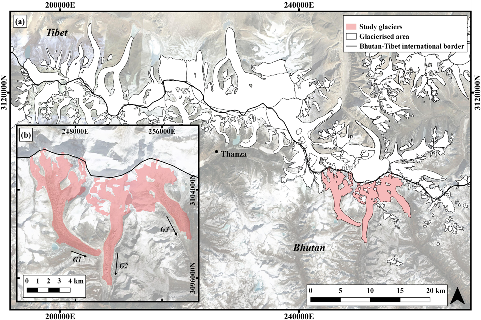
Fig. 1. (a) Glacierised area within the study region along the Bhutan–Tibet border, showing the glaciers (red). The inset (b) shows the three selected debris-covered glaciers (from left to right; G1, G2 and G3). Background: Planet Labs image from 24 January 2018.
2.2 Data sources
We used 49 images derived from level 3B tiles collected by the PlanetScope One Satellite constellation (3 m resolution) between January 2016 and December 2018 (Table S1, Fig. 2; https://www.planet.com/). Due to data availability, we supplement these data with eight scenes derived from RapidEye Ortho-tiles (5 m resolution) from January 2016, February 2016 and January 2017. These images constituted all the clear-sky (<5% cloud coverage over the glacier area) images over the three glaciers. To assess the seasonal pattern of pond formation and drainage, images were selected from each season according to Steiner and others (Reference Steiner, Buri, Miles, Ragettli and Pellicciotti2019): winter (1 December to 28 February), pre-monsoon (1 March to 15 June), monsoon (16 June to 15 September) and post-monsoon (16 September to 30 November). Due to the limited data availability, the number of images per season, per year and per glacier vary. For winter, we have images for every month and year, so we have high confidence in the associated patterns. Coverage for post-monsoon was near-complete, missing one data point from September 2016 for all three glaciers. Pre-monsoon and monsoon were far more sporadic, which is a common problem with optical remote-sensing studies in monsoonal regions where dense cloud-cover and snow cover limits observations (Miles and others, Reference Miles2017). G3 had one pre-monsoon season image and one monsoon season each year, whereas G1 and G2 were only imaged in 2017 and 2018. Given pre-monsoon was represented by one month on one glacier only (G3) we have excluded pre-monsoon from our analysis. We acknowledge this sporadic temporal coverage potentially causes bias issues in the monsoon season and discuss this within the text.
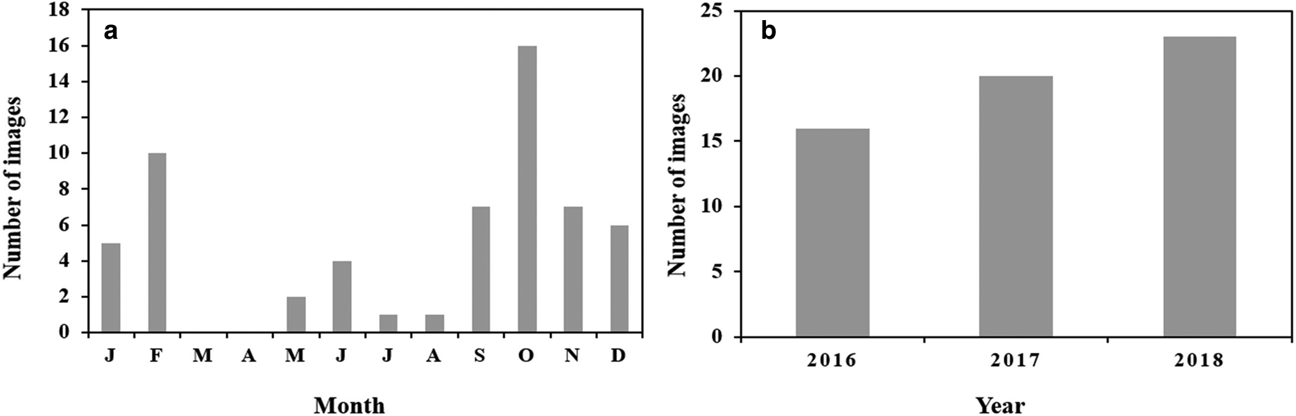
Fig. 2. Temporal distribution of scenes processed in the study, with the number of images per month: (a) and per year and (b) (n = 56).
2.3 Supraglacial ponds
The normalised difference water index (NDWI) (McFeeters, Reference McFeeters1996) uses the ratio between the near-infrared and green bands to separate areas of water and non-water, and has been successfully used to delineate supraglacial ponds in the Langtang and Everest regions of Nepal (e.g. Bolch and others, Reference Bolch, Buchroithner, Peters, Baessler and Bajracharya2008; Bolch and others, Reference Bolch, Pieczonka and Benn2011; Kraaijenbrink and others, Reference Kraaijenbrink, Shea, Pellicciotti, De Jong and Immerzeel2016). We use Otsu's adaptive histogram-based method to select an optimised NDWI threshold for each scene (Otsu, Reference Otsu1979; Cooley and others, Reference Cooley, Smith, Stepan and Mascaro2017). This method iterates through all the possible threshold values, calculates a measure of spread for the pixels on each side of the threshold and selects the threshold value where the spread of pixels in the foreground and background is at its minimum. The resulting threshold was then used to reclassify the study imagery into a binary image of ponds (1) and anything else (0) (Fig. 3). Threshold values between 0.3 and 0.4 produced the most accurate identification of supraglacial ponds, with minimal omissions. The resultant binary image was converted to polygons, with each polygon representing an individual supraglacial pond (Fig. 3c). Polygons produced via the NDWI threshold were manually adjusted where required, e.g. where ponds were frozen, partially frozen and/or had a high sediment content (Fig. 3d). Each mapped pond was given an ID, enabling ponds that drained to be matched despite the change in location due to glacier velocity.
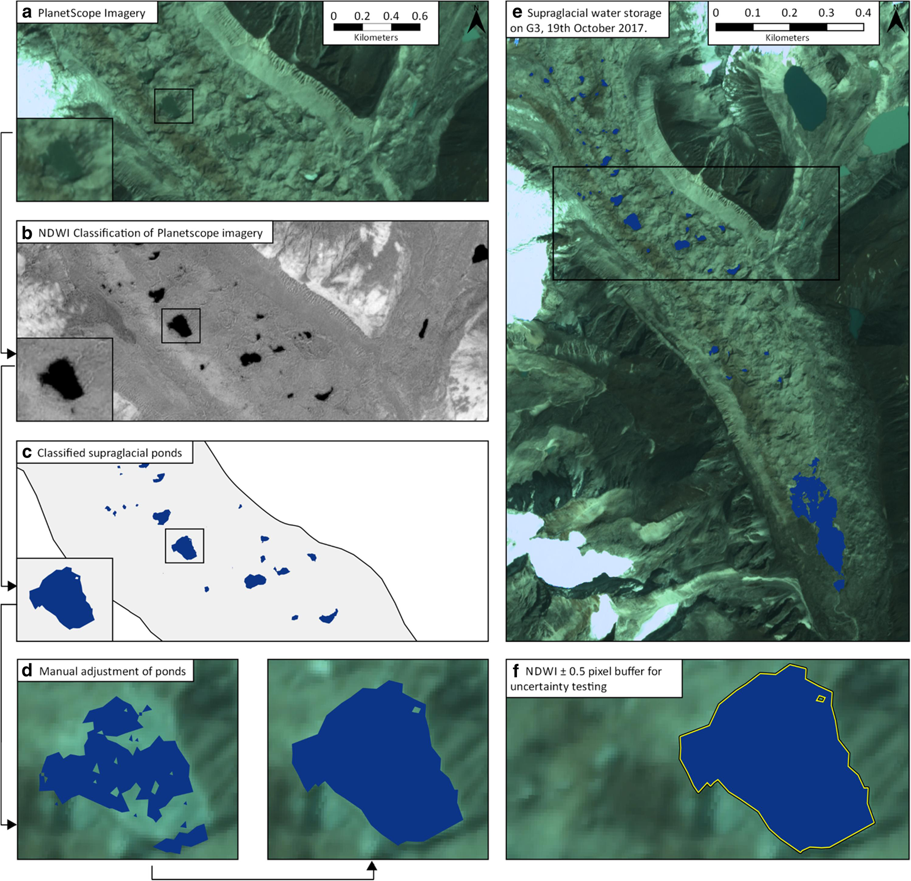
Fig. 3. Workflow of pond classification using the NDWI method on PlanetScope. (a) Original PlanetScope mosaic, (b) NDWI to delineate surface water, (c) classified supraglacial pond polygons, (d) manual adjustment of pond polygons due to floating ice/sediment content/boundary conditions, (e) final identified supraglacial ponds on G3 (19th October 2017) and (f) half pixel uncertainty assessment. Background image: Planet Labs, 19/10/2017.
To identify any differences in the ponds mapped on both RapidEye and Planet Labs images, we compared our NDWI classification for two images from the same date and found the area of supraglacial ponds agreed well; on average ponds mapped on RapidEye images had an area 4.8% greater than the same ponds mapped on Planet Labs images. Hence, the use of RapidEye images has minimal impact on our lake area statistics (Fig. S1). We estimate total uncertainty for the automatically identified ponds using a ±0.5 pixel boundary (e.g. Salerno and others, Reference Salerno2012; Wang and others, Reference Wang, Siegert, Zhou and Franke2013), which estimates the average error to be 28%. We checked the accuracy of this assumed ±0.5 pixel boundary by manually delineating a subset of 58 supraglacial ponds of different sizes. The area of all 58 manually digitised and automatically identified ponds agreed well (Fig. S2b). The average error, expressed as a percentage of total area, was 7.0%. This indicates that we conservatively estimate uncertainty using the pixel boundary approach.
2.4 Ice cliffs
Ice cliffs were manually delineated using the same satellite imagery as for the ponds. Here, we define ice cliffs as any exposed, sloping ice, whether that be clean ice or ‘dirty’ ice (i.e. a thin layer of debris may cover all or part of the cliff). The top-edge of ice cliffs on each of the glacier surfaces was manually digitised in a left to right direction with the cliff facing outwards. We delineated the top-edge of the ice cliffs to determine their length and orientation but did not estimate area since this requires a high-resolution digital elevation model (Watson and others, Reference Watson, Quincey, Carrivick and Smith2017a). Previous study suggests that ponds with bordering ice cliffs experience higher rates of expansion (e.g. Watson and others, Reference Watson, Quincey, Carrivick and Smith2016); however, since cliffs are near vertical, it is difficult to determine whether a pond intersects with a cliff using only the top-edge of the ice cliff. Therefore, we used a 30 m directional buffer from the top-edge of each cliff to determine if the ice cliff was in contact with a pond (Fig. S3). Direction was assumed from the side facing or in contact with the pond itself, and any pond within this buffer was said to have an adjacent cliff. Ice cliffs can only persist where you have clean ice or ice with a very thin debris veneer. Therefore, cliffs have to be at or above the angle of repose to form. Thus, the 30 m buffer is derived from the average debris angle of repose of 30° (e.g. Sakai and others, Reference Sakai, Nakawo and Fujita1998), and using an approximated upper bound for a steeply sloping cliff face of 15 m (Benn and others, Reference Benn, Wiseman and Hands2001; Thompson and others, Reference Thompson, Benn, Mertes and Luckman2016).
Uncertainty in ice cliff length is determined by the resolution of the images used for digitisation, operator misidentification of cliffs and operator digitisation of the cliffs (Watson and others, Reference Watson, Quincey, Carrivick and Smith2017a). Given that high-resolution imagery was used, and one operator undertook all the analysis, the manual digitisation is likely the largest source of error. To quantify these errors, 50 of the total 2088 cliffs were randomly selected and re-digitised (Fig. S2a). The original and repeat cliff lengths showed good agreement; lengths of repeat-digitised cliffs were on average no more than 3.0% different to that of the original cliffs. The difference between the two had a low std dev. (4.3 m) indicating that the manual digitising error was low.
2.5 Controls on pond formation
We assessed how glacier surface velocities affect supraglacial pond formation and growth. Glacier surface velocities (120 m resolution) were provided by the NASA MEaSUREs ITS_LIVE project (Gardner and others, Reference Gardner, Fahnestock and Scambos2019), generated using the auto-RIFT feature tracking processing chain described in Gardner and others (Reference Gardner2018). For each glacier, velocity profiles were extracted along the glacier's centreline in 500 m horizontal bins from the terminus up-glacier. These binned velocities were used to compare pond locations and surface velocities for the three glaciers. Considerations of debris thickness and surface slope are also included in the discussion however not analysed in detail here. Thickness estimates were provided by Rounce and others (Reference Rouncein review) and slope determined using the HMA 8 m DEM (Shean, Reference Shean2017).
3 Results
3.1 Supraglacial pond changes
3.1.1 Spatial and temporal pond variations between glaciers
Average pond area in the study region was 1206 m2, with ponds on G3 on average the largest (1645 m2) and ponds on G2 the smallest (805 m2). The total ponded area for our three glaciers between January 2016 and December 2018 varied considerably spatially and seasonally (Table 1; Fig. 4). G1 had the highest average ponded area of 175 855 m2, which was 3.5 times more than that of G2 (49 329 m2) and 1.5 times more than that of G3 (116 969 m2). Similarly, the average number of ponds on G1 (156) was 2.5 times more than those on G2 (62) and two times more than those on G3 (78). G2 consistently had the lowest ponded area and pond number. During the study period, all three glaciers demonstrated marked temporal variations in ponded area, with G3 having the largest range at almost 200 000 m2. G1 had the largest range with respect to numbers of ponds (100). There was an overall decrease in the percentage ponded area on G1 and G2 between January 2016 and December 2018.
Table 1. Supraglacial pond changes during 2016–18 for the three glaciers
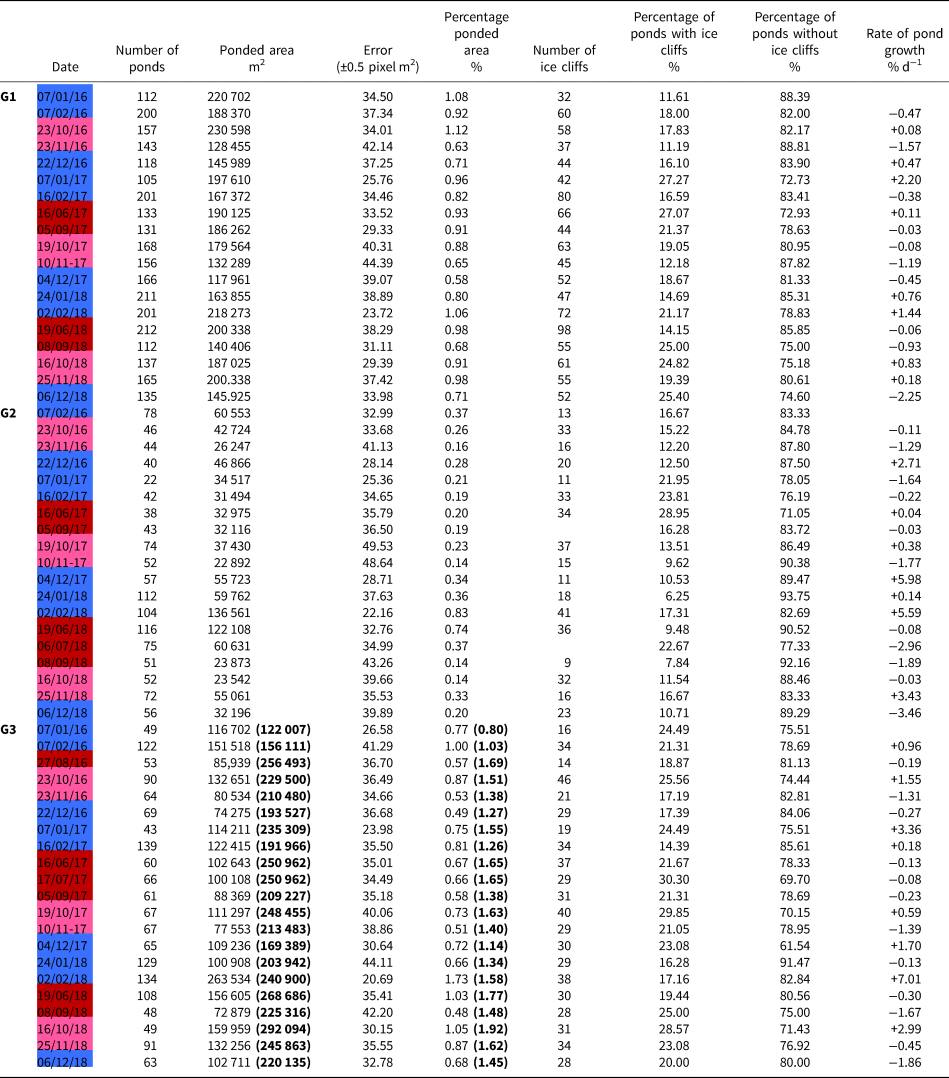
Dates are coloured by season; blue (winter), red (monsoon) and pink (post-monsoon). Values in brackets for Glacier 3 represent the area of pond G3-A.
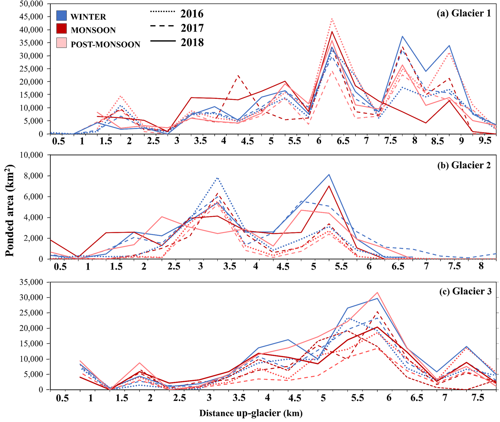
Fig. 4. Spatial and temporal changes during 2016–18 for the three glaciers showing ponded area change with distance up-glacier from the terminus for glaciers (a) G1, (b) G2 and (c) G3. Profiles are derived from ponded area per 500 m distance bins. Note that ponded area tends to increase with distance up-glacier, but with high degree of variation between seasons.
Seasonal variations on G2 and G3 showed that the ponded area was higher during the winter season (Fig. 4). Specifically, the average ponded area was 5.0 and 21.3% higher in the winter than in the monsoon season average, and 39.28 and 9.89% higher than the post-monsoon average, respectively. In contrast, the average ponded area on G1 during the monsoon season (179 280 m2) was 3.0% higher than that in winter season (174 006 m2) and 1.6% higher than that in post-monsoon season (176 340 m2; Fig. 4). These spatio-temporal variations clearly show glacier to glacier variation in ponded area, number and seasonality, despite their close proximity.
The percentage ponded area (defined as percentage of the total debris-covered glacierised area occupied by supraglacial ponds) also varied over the study period for all three glaciers (Table 1). G2 had the lowest percentage ponded area, ranging from a minimum of 0.3% in November 2017 to a maximum of 1.7% in February 2018. The largest range in percentage ponded area was found on G3, which varied from 1.0% in September 2018 to 3.5% in February 2018. The highest percentage ponded area was recorded on G2 and G3 in February 2018, which experienced an increase between January 2018 and February 2018 of 0.7 to 1.7% on G2 and 1.4 to 3.5% on G3. The rate of pond growth on each glacier changed over the study period; however, no significant overall trends can be observed due to the sporadic temporal coverage (Fig. S4 and Table 1).
3.1.2 Spatial patterns of ponding across glaciers
Generally, the spatial patterns of supraglacial ponding remained similar throughout the study period for all three glaciers, subject to seasonal variations (Fig. 4). On G2 and G3, pond number and ponded area were generally higher of 4 and 6 km up-glacier, with fewer ponds found near the glacier termini or at higher elevations (Fig. 7). However, on G3, during the winter, ponded area increased further up-glacier (above 6 km), while during the monsoon season ponding increased on the lower glacier (below 4 km from the terminus). A similar trend was observed on G2, with a shift from mid-glacier ponding during the winter season to lower-glacier ponding during the monsoon season (Fig. 4b). The spatial pattern of ponding on G1 differs from the other glaciers, with two distinctive zones of higher ponded area and number (zone 1: km up-glacier; zone 2: above 7.5 km up-glacier) separated by a zone with lower ponded area and number of ponds (note: while not physically separated we have distinguished the two ‘zones’ based on the different observed spatial distribution of surface ponds as separating them aids interpretation). This divide is evident throughout the study period (2016–18) with notably fewer ponds between 7.0 and 7.5 km up-glacier (Fig. 4a). Similar to G2 and G3, ponded area and number increased on the lower glacier on G1 during the monsoon season. Persistence and coalescence of ponds through the study period means G1 is developing a chain of connected ponds on its eastern margins at 0.5–2.5 km up-glacier.
3.1.3 Pond drainage
Our data provide evidence for both pond drainage and persistence. Here, we define drainage as the disappearance and reappearance of a pond in the same location between imaging periods, i.e. one complete drainage and refill. Most ponds persisted between seasons and years (98.2% of the total ponds detected during the study period persisted), while a total of 103 (1.8%) ponds drained and refilled (Fig. 5). The most drainage and refill events occurred on G1 (34) and the least on G2 (14). Of these 103 drainage and refill events, 52 occurred once, 21 twice and only three ponds underwent three complete drainage and refill cycles during the study period (two on G1 and one on G3). We find no limit to the size of ponds that drain. Although these drain-and-fill events occurred across each glacier, they were generally located on the middle to upper portion of G1 and G3 (i.e. above 5 and 4 km up-glacier, respectively). Only four ponds drained in the first 5 km on G1, whereas all 28 drainage events on G3 occurred above 3.6 km up-glacier. In comparison, all 14 drainage events on G2 occurred in the middle or lower portion of the glacier, below 5.6 km up-glacier. On average, the most frequent season for ponds to drain was the monsoon, with 51 recorded events (equivalent of eight per month during the monsoon months) with the other two seasons experiencing the same frequency (three per month) (Fig. 5). Given the sporadic data coverage during monsoonal periods, there is uncertainty here.

Fig. 5. (a) Location of ponds experiencing drainage and refill on the three glaciers during 2016–18. Ponds were found to drain once (blue), twice (pink) or three times (yellow). Note drainage generally occurs mid-to-high glacier on all three glaciers. (b) and (c) Total number and number per month of drainage and refill events according to seasonal distribution. The monsoon season is the only period in which we see a marked increase in drainage frequency over the study period as a whole, however the lower number of observations during this period means there is uncertainty in this finding. Background image: Planet Labs, 19/10/2017.
3.1.4 Pond G3-A
Pond G3-A, a large supraglacial pond on the lower terminus of G3 was assessed separately from the other supraglacial ponds due to its large size. G3-A underwent a net gain of 98 120 m2 (87.6% increase) over the study period, varying 122 010 m2 in January 2016 to 220 130 m2 in December 2018 (Table 1). Ponded area also varied seasonally with the area generally smaller in the monsoon and post-monsoon and larger in the winter. No drainage events were observed for G3-A during the study period.
3.2 Ice cliff changes
3.2.1 Spatial and temporal ice cliff variations between glaciers
The number and spatial distribution of ice cliffs varied markedly between seasons, years and glaciers (Fig. 6). The highest number of ice cliffs were found on G1, ranging from 32 in January 2016 to 98 cliffs in June 2018. The lowest number were found on G2, ranging from nine in September 2018 to 41 in February 2018 (Fig. 6; Table 1). Most ice cliffs were located between the middle of the glacier and the terminus on all three glaciers. However, a large cluster of ice cliffs occurred at higher elevations on G1. The number of ice cliffs on G3 was the most consistent during the study period, with a std dev. of 7.5 (compared to 15.7 and 10.8 for G1 and G2 respectively; Table 1). For all three glaciers, ice cliffs generally persisted from year to year, with increases in number resulting from the formation of new cliffs, and decreases in number the result of the joining, of existing ice cliffs, rather than decay.
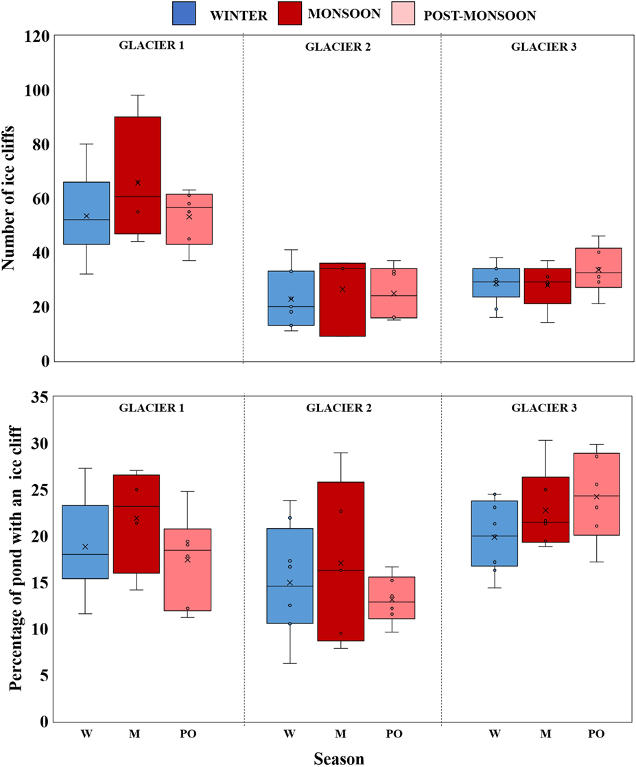
Fig. 6. (Top) Variation in the number of ice cliffs and (bottom) percentage of ponds with an ice cliff found on all three glaciers during 2016–18 for winter (blue), (red) and post-monsoon (pink). Note the box ranges highlights the lack of significant differences between seasons.
The average number of ice cliffs per glacier showed only a slight temporal pattern, with the average being higher during the monsoon season than in the post-monsoon and winter season on both G1 and G2. G1 averaged 66 during the monsoon and 53 during both post-monsoon and winter, whereas G2 averaged 26 in the monsoon and 25 and 23 post-monsoon and winter, respectively (Fig. 6; Table 1). In contrast, on G3, there were more cliffs on average post-monsoon (36 cliffs) than during winter and monsoon (28 cliffs each; Fig. 6). Note this difference could be due to temporal bias in observation periods, rather than an indication of seasonality. The orientation of ice cliffs was not analysed in detail for this study and thus has not been included. However, throughout all seasons cliffs generally favoured a north or northwest direction. The frequency of south, southeast and east facing cliffs was few to none, but increased marginally during monsoon season.
3.2.2 Pond–cliff coincidence
There were far more supraglacial ponds without a corresponding ice cliff than with. On average, only 19.0% of supraglacial ponds had a coincident cliff during the study period. The highest pond–cliff coincidence was found on G3, ranging from a minimum of 14.0% in February 2017 to a maximum of 29.0% in October 2017, and the lowest on G2, averaging 15.0% over the period January 2016 to December 2018. During the study period, the percentage of ice cliffs associated with a supraglacial pond increased on G1 by +14.0% and decreased on G2 by 6.0% and on G3 by 4.0% (Table 1). Seasonal changes in percentage of ponds with an adjacent ice cliff varied by <3.0%, suggesting limited influence here.
3.3 Glacier surface velocities
Glacier surface velocity on all three glaciers generally decreased towards the terminus (Fig. 7). Velocities were substantially higher on G1 in 2018, compared to previous years, and slightly higher at certain locations along the profiles of G2 and G3. With one exception, all drainage and refill events on G1 and G2 occurred in locations where glacier surface velocities were above 8.0 m a−1. In contrast, 14 (60.0%) of the drainage events on G3 occurred in areas with surface velocities between 4.0 and 8.0 m a−1 and three events were in areas flowing at <4.0 m a−1. There was no apparent difference in ice velocities for ponds that drained once versus twice, but ponds that experienced three complete drainage and refill cycles were all located in areas of where glacier surface velocities were >10.0 m a−1.
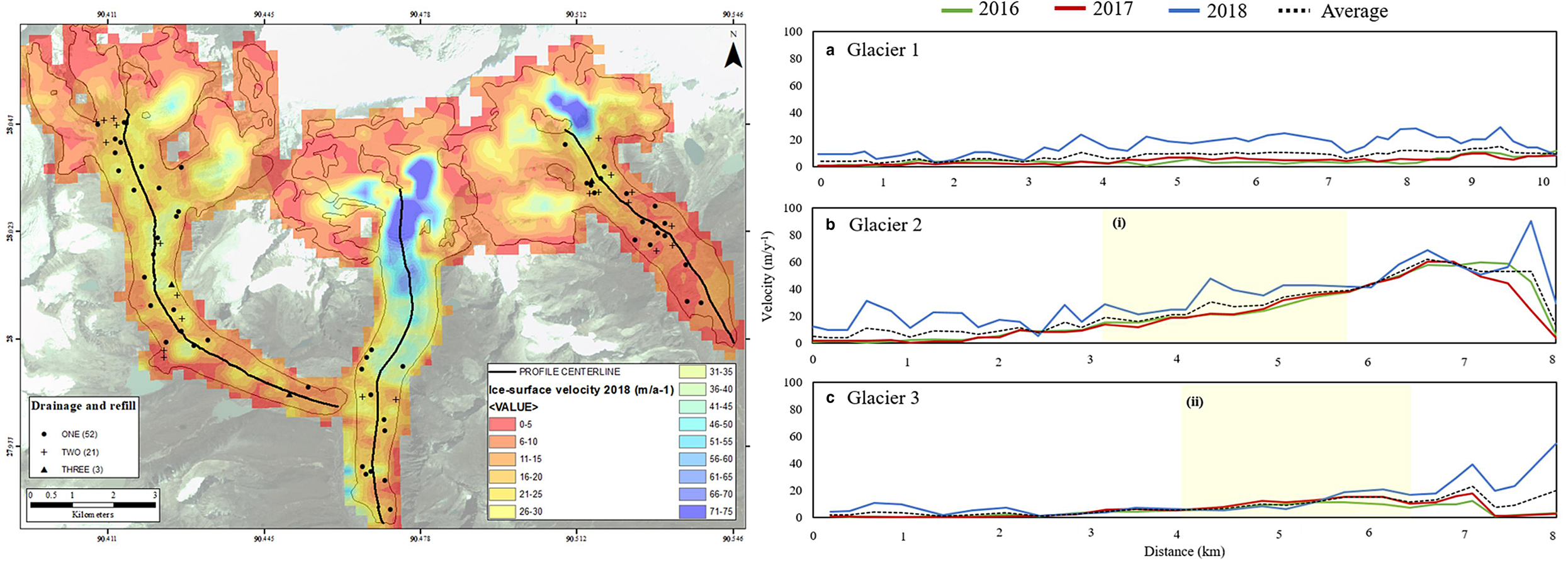
Fig. 7. (a) Location of pond drainage and refill events with ice surface velocities for 2018. Although most ponds are found in areas where velocity is <8 m a−1 the majority of pond drainage events occurred where velocities are above 8 m a−1. A few drainage events on G3 are exception to this rule, occurring where velocity is <8 m a−1. (b, c) Glacier ice surface velocities for 2016, 2017, 2018 and average for the study period from the terminus (0 km) up-glacier (8/10 km). Profiles were derived from the centreline of each glacier. Yellow sections (i) and (ii) highlight locations of higher frequency ponding, mentioned in text (Section 3.1.2).
4 Discussion
4.1 Seasonal variation in supraglacial pond development
4.1.1 Temporal variation
Over the study period, ponded area varied between months and years, as well as in location across the glacier surface, with ponded area on G1 behaving differently than ponded area on G2 and G3 (Fig. 4). Specifically, ponded area on G1 increased during the summer months, whereas it increased in winter on G2 and G3. This is unexpected, given their proximity and therefore similar climate forcing. We attribute ponded area expansion on G1 during summer to a combination of precipitation inputs from the Indian Summer Monsoon and increased meltwater generation during the summer ablation season (e.g. Irvine-Fynn and others, Reference Irvine-Fynn2017; Miles and others, Reference Miles2017). Similar summer expansion has observed in previous studies, on the Langtang Glacier, Nepal (Miles and others, Reference Miles, Willis, Arnold, Steiner and Pellicciotti2016), in the Tien Shan (Narama and others, Reference Narama2017) and in the Khumbu region, Nepal (Watson and others, Reference Watson2017b). Most of the observed drainage events occurred on G1 (45.0%) and were during the summer season (Fig. 5). We suggest this is due to an increase in available meltwater and/or rainfall, causing ponds to form on the glacier surface. These ponds then represent areas of high hydraulic potential that can more readily exploit englacial conduits to areas of lower hydraulic potential and drain into the glacier (Benn and others, Reference Benn2017; Miles and others, Reference Miles2017). Upon drainage, thermal energy stored within the pond water is transferred to the glacier interior and can thus enhance mass loss due to englacial ablation (e.g. Sakai and others, Reference Sakai, Takeuchi, Fujita and Nakawo2000; Miles and others, Reference Miles, Willis, Arnold, Steiner and Pellicciotti2016; Watson and others, Reference Watson2017b).
Pond area at G2 and G3 increased during the winter months (Fig. 4), which is unusual given the enhanced precipitation, pond ablation, meltwater generation and increased pond connectivity with the englacial drainage system that is usually observed during the summer months on eastern Himalayan glaciers (e.g. Sakai and others, Reference Sakai, Takeuchi, Fujita and Nakawo2000; Wang and others, Reference Wang, Liu, Han, Wang and Liu2012; Miles and others, Reference Miles, Willis, Arnold, Steiner and Pellicciotti2016; Watson and others, Reference Watson, Quincey, Carrivick and Smith2016, Reference Watson2017b). Additionally, precipitation is usually limited in winter and temperatures remain low (Mool and others, Reference Mool2001; Hoy and others, Reference Hoy, Katel, Thapa, Dendup and Matschullat2016). Both G2 and G3 have braided networks of streams on the glacier surface during the monsoon season (Figs 8c, e) that are no longer active by the following winter (Figs 8d, f). Compared to the terminus of G1, the surface hydrology connectivity is much less established during the summer (Fig. 8a). Therefore, we suggest the established outlet channels on G2 and G3 may be efficient in removing the excess seasonal meltwater from the surface during the summer. As meltwater supply reduces and ponds begin to freeze over during winter, the outlet channels become less efficient, leading to higher ponded area during the winter months compared to the summer period. In comparison, the poorly connected supraglacial hydrological system on the terminus of G1 may be promoting surface storage. The steeper profiles and generally higher velocities of G2 and G3 compared to G1 would facilitate this effective surface transport. Our findings therefore suggest that the efficiency of the supraglacial hydrological system at all three glaciers evolves between summer and winter, but in different ways. Under a warming climate, we might expect efficient surface drainage to persist at G2 and G3 and thus ponded areas to remain small, whereas on G1, we might expect ponded area to increase with warming. It is worth noting that recent studies have revealed that thermal energy is stored within ponds overwinter, trapped in by an insulating layer of snow-covered ice (e.g. Watson and others, Reference Watson, King, Miles and Quincey2018). Thus, further analysis of pond thermal regime would be needed to determine drivers. Additionally, the lack of pre-monsoon and sporadic monsoon data may be masking some changes during the summer months.

Fig. 8. Outlet stream networks on the glacier termini: (a) G1 monsoon, (b) G1 winter, (c) G2 monsoon, (d) G2 winter, (e) G3 monsoon and (f) G3 winter. Note the outlet streams are more developed during the monsoon season than the winter season. Background images are binary PlanetScope images after application of NDWI; monsoon; 05/09/17 and winter; 02/02/18.
4.1.2 Spatial variation between glaciers
On our glaciers, ponds clustered in the mid-ablation zone (Fig. 4), which we attribute to the impact of debris cover on glacier dynamics. Debris cover is generally thinner (<0.25 m) further up-glacier on all three glaciers (Fig. S5), and therefore the underlying ice experiences more melt compared to clean-ice at higher elevations or ice insulated by thicker debris close to the terminus or glacier margins As such, the mid-ablation zone generally experiences the highest melt rates (Watson and others, Reference Watson2017b), which can reduce glacier surface gradients, promote glacier stagnation (e.g. Quincey and others, Reference Quincey, Richardson, Luckman, Lucas, Reynolds, Hambrey and Glasser2007; Miles and others, Reference Miles2017; Steiner and others, Reference Steiner, Buri, Miles, Ragettli and Pellicciotti2019) and initiate ponding. In areas where debris cover is thicker (>0.5; Fig. S5), ponding is less frequent. This is further supported by our velocity data, which show that the mid-ablation zone glacier velocities on G1 and G2 were below 10.0 m a−1 and below 15.0 m a−1 on G3 suggesting a reduction in glacier flow. Although the local surface slope is generally below 20° in this mid-ablation zone, there is substantial variation observed across all three glacier surfaces (Fig. S6). As such, the role of surface slope in supraglacial pond and ice cliff formation here remains unclear.
The number of ponds and ponded area were consistently higher on G1 than on the other two glaciers (Table 1). This may be due to G1's lower surface velocities (Fig. 7), where between 2016 and 2018 average surface velocities remained below 10.0 m a−1 across G1's tongue; compared to G2 and G3, where velocity did not fall below 10.0 m a−1 until the mid-ablation area (5.6 km up-glacier on G2, and 6.2 km up-glacier on G3). Ponds usually begin to form where velocities are <10.0 m a−1 (e.g. Quincey and others, Reference Quincey, Richardson, Luckman, Lucas, Reynolds, Hambrey and Glasser2007; Miles and others, Reference Miles2017), meaning that the area in which ponds are able to form on G1 is greater, leading to the overall higher number of ponds and ponded area. However, G2 and G3 have low ice-surface velocities within ~3.0 and 5.0 km of their termini, respectively (Fig. 7), which may help to explain why we see higher winter ponded areas on G2 and G3, i.e. low glacier velocities may produce an inefficient englacial drainage system, which would inhibit drainage and promote supraglacial ponding (e.g. Jordan and Stark, Reference Jordan and Stark2001; Benn and others, Reference Benn2012, Reference Benn2017). Future research looking at this relationship with higher resolution velocity data would be useful here. If ponds persist through seasons rather than draining and refilling, surface melting may increase, as ponds will absorb atmospheric energy for longer (Mertes and others, Reference Mertes, Thompson, Booth, Gulley and Benn2016; Miles and others, Reference Miles2017). The transition from supraglacial ponds into proglacial lakes has been observed since the 1950s in the Lunana region of Bhutan, where three of the country's largest proglacial lakes are located (Luggye Tsho, Thorthormi Tsho and Raphstreng Tsho). Should the supraglacial ponds found in this study begin to coalesce, as has been observed elsewhere (e.g. Richardson and Reynolds, Reference Richardson and Reynolds2000; Quincey and others, Reference Quincey, Richardson, Luckman, Lucas, Reynolds, Hambrey and Glasser2007; Thompson and others, Reference Thompson, Benn, Dennis and Luckman2012; Mertes and others, Reference Mertes, Thompson, Booth, Gulley and Benn2016; Watson and others, Reference Watson, Quincey, Carrivick and Smith2016) the risk of proglacial lake development at the terminus of these glaciers, and thus potential for glacial lake outburst floods will increase.
4.1.3 Spatial variation on individual glaciers
We observed a shift in the spatial pattern of ponding from the mid-ablation zone to lower altitudes during the monsoon season, whereas ponded area increased at higher altitudes during the winter season (Fig. 4). This spatial shift down-glacier contrasts with the Everest region of Nepal, where the location of ponds shifted up-glacier during the summer months, while pond frequency in the lower ablation zone remained low (Watson and others, Reference Watson, Quincey, Carrivick and Smith2016). Watson and others (Reference Watson, Quincey, Carrivick and Smith2016) suggest this shift was due to the presence of well-connected surface hydrological systems that allow meltwater to be efficiently conveyed to the outlet during the summer months. The most pronounced spatial shift in our study was on G1, which supports our suggestion that G1 has less connected supraglacial hydrological systems in its lower ablation area. Hence, seasonal meltwater is not efficiently transported to the outlet and instead collects in topographic inversions, resulting in higher frequency ponding in the lower-ablation area.
The spatial pattern of ponds on G1 is similar overall to the other two glaciers, but also had a zone of lower ponded area/number of ponds 7.0–7.5 km up-glacier (Fig. 4). There are no notable changes in glacier-surface velocity at this point (Fig. 7), there is no real change in the colour or composition of the surface debris cover (Fig. 1), nor debris thickness (Fig. S5). We therefore suggest this area of limited ponding may be due to the surrounding topography. Here, a smaller source tributary from the northeast joins the trunk from the north, and the surrounding topography becomes steeper (Fig. S7). This may alter the amount of shortwave radiation reaching the glacier surface due to increased shadowing (e.g. Steiner and others, Reference Steiner2015), thereby reducing ablation, and thus ponding. Below this area, where the topography is less steep, shadowing is reduced and thus higher rates of ablation are experienced as more shortwave radiation is directly transmitted to the glacier surface, and for longer. Studies have suggested that surrounding topography can also expose glacial ice to more longwave- and reflected shortwave-radiation (e.g. Steiner and others, Reference Steiner2015). Thus, it is possible that other factors are inhibiting pond formation in this area, such as a change in wind direction (altering waterline advection and therefore impacting marginal melt) or the presence of efficient drainage networks, which warrant further investigation.
4.1.4 Pond drainage
Glaciers in Bhutan are summer accumulation type glaciers, i.e. they receive precipitation inputs during the ablation season, which corresponds with the middle of the Indian Summer Monsoon (Bookhagen and Burbank, Reference Bookhagen and Burbank2010; Wagnon and others, Reference Wagnon2013). Thus, glaciers are both gaining and losing mass simultaneously, which leads to increased meltwater generation that can either be retained in ponds or drained via supraglacial meltwater channels and/or englacial conduits. On all three glaciers, the most drainage events (51 events) occurred during the monsoon season, with an average of eight events per month during the monsoon season compared to just three per month in the remaining seasons (Fig. 5). This coincides with when increased meltwater supply opens conduits, thereby making englacial drainage more efficient (Miles and others, Reference Miles, Willis, Arnold, Steiner and Pellicciotti2016; Irvine-Fynn and others, Reference Irvine-Fynn2017). Due to the limited data coverage during the monsoon season, and data gap from the pre-monsoon season we cannot determine if this difference is significant. More confidence can be placed on trends seen for post-monsoon and winter periods given the near-continuous data coverage during these periods.
G1 experienced more drainage events (34) than the other two glaciers (14 on G2 and 28 on G3) (Fig. 5), but the percentage of the number of ponds that drained was higher on G2 (23.0%) and G3 (35.0%) than on G1 (22.0%). Supraglacial ponds that repeatedly drain convey energy to the glacier interior, which can enhance englacial melt rates and lead to conduit roof collapse and the nucleation of further supraglacial ponds in the resulting depressions (e.g. Sakai and others, Reference Sakai, Takeuchi, Fujita and Nakawo2000; Mertes and others, Reference Mertes, Thompson, Booth, Gulley and Benn2016; Miles and others, Reference Miles, Willis, Arnold, Steiner and Pellicciotti2016, Reference Miles2017). Thus, these drainage events may be contributing to the overall higher ponded area and number of ponds seen on G1 as there are more topographic depressions for meltwater to accumulate. G2 and G3 experienced fewer drainage events than G1, supporting the idea that both glaciers have established supraglacial hydrological systems that deliver ponded water to the proglacial environment, rather than draining via englacial conduits. In contrast, the inefficient surface hydrological system on G1 (Fig. 8) may allow ponded area to increase, which increases the chances of englacial drainage, as ponds expand via horizontal and lateral melting (e.g. Benn and others, Reference Benn, Wiseman and Hands2001).
On debris-covered glaciers, widespread downwasting of glacier surfaces results in reduced driving stresses and thus reduced glacier surface velocities (Benn and others, Reference Benn2012). In locations where velocities are low, inefficient englacial drainage pathways exist, promoting the development of supraglacial ponds (Jordan and Stark, Reference Jordan and Stark2001; Benn and others, Reference Benn2012, Reference Benn2017); hence, glacier surface velocities drive patterns of pond drainage or persistence and determine pond size (e.g. Miles and others, Reference Miles2017). We therefore expect a higher number of ponds and larger ponded area where surface velocities are lower (e.g. Thompson and others, Reference Thompson, Benn, Mertes and Luckman2016; Miles and others, Reference Miles2017; Watson and others, Reference Watson2017b). Our results support this, with a higher ponded area and number of ponds found in areas where surface velocities <10.0 m a−1, and drainage and refill events generally occurring where surface velocities were >8.0 m a−1 (Fig. 7). Furthermore, comparatively higher surface velocities on G1 in 2018 (Fig. 7) corresponds with a decline in both the number and area of supraglacial ponds across the whole glacier (Table 1, Fig. 4), suggesting velocity may play a key role in pond formation and decay here. Ponds with multiple drainage events were associated with substantially higher ice velocities, which would facilitate englacial conduit opening. As such, surface velocities appear to be an important control on pond drainage and persistence on our glaciers, with drainage generally occurring in areas with velocities above 8.0 m a−1.
4.1.5 Pond G3-A
Pond G3-A behaved differently than the other supraglacial ponds on G3 as the ponded area was higher during the monsoon season than in any other season. This contrasts with our other observations, where ponded area generally decreased during the monsoon season. We observed no drainage events at pond G3-A during the study period, with the only drainage occurring via an established outlet channel that connects to the proglacial environment. The lack of observed drainage events and continuous filling indicates that pond G3-A has no efficient connection to the englacial system and/or is at or below hydrological base level, allowing for continued expansion (e.g. Quincey and others, Reference Quincey, Richardson, Luckman, Lucas, Reynolds, Hambrey and Glasser2007; Benn and others, Reference Benn2012; Mertes and others, Reference Mertes, Thompson, Booth, Gulley and Benn2016; Thompson and others, Reference Thompson, Benn, Mertes and Luckman2016). There is a possibility based on the consistent expansion observed here that G3 may develop into a proglacial lake in the future (Richardson and Reynolds, Reference Richardson and Reynolds2000; Bolch and others, Reference Bolch, Buchroithner, Peters, Baessler and Bajracharya2008). However, we refrain from speculating here as it may lead to misinformation. Instead, we recommend the pond be closely monitored to forecast future risks to downstream populations, including area and hydrological changes of the pond itself, as well as structural changes at the glacier terminus moraines.
4.2 Ice cliffs
4.2.1 Ice cliff distribution
The majority of cliffs were located between the glacier termini and the mid-ablation area, as with the supraglacial ponds (Fig. S8). This spatial distribution mirrors that in the Everest region (e.g. Watson and others, Reference Watson, Quincey, Carrivick and Smith2017a; Steiner and others, Reference Steiner, Buri, Miles, Ragettli and Pellicciotti2019), and remains similar throughout the year, suggesting that seasonal-scale controls have less impact on ice cliffs than they do on ponds. Ice cliffs form due to the slope steepening past the angle of repose or through englacial roof collapse (e.g. Kirkbride, Reference Kirkbride1993; Sakai and others, Reference Sakai, Takeuchi, Fujita and Nakawo2000; Reid and Brock, Reference Reid and Brock2014). We might therefore expect to find cliffs in both faster-flowing ice, due to crevassing and thus slope steepening, and slower-flowing ice, due to pond expansion and subsequent englacial collapse. However, we found no clear association between ice cliffs and surface velocities, with cliffs existing at a range of glacier surface velocities (Fig. 7 and Fig. S8). Notably, in slow-flowing zones (<4.0 m a−1) ice cliffs continued to form and decay, potentially through conduit collapse. This suggests that surface velocities have a limited influence on the location of ice cliffs on our glaciers, in contrast to their influence on pond locations.
4.2.2 Spatial coincidence of ice cliffs and supraglacial ponds
Recent studies indicate that ice cliffs and supraglacial ponds tend to form in the same locations and due to the same controlling factors (e.g. Watson and others, Reference Watson, Quincey, Carrivick and Smith2017a; Steiner and others, Reference Steiner, Buri, Miles, Ragettli and Pellicciotti2019). However, our data show that of the total number of supraglacial ponds, only 19.0% coincided with an ice cliff which is markedly lower than other regions of the Himalaya, with estimates for the Everest region ranging between 49.0 and 74.0% of the total pond number (Thompson and others, Reference Thompson, Benn, Mertes and Luckman2016; Watson and others, Reference Watson, Quincey, Carrivick and Smith2017a). One potential explanation may be the rapid rates of pond expansion and high frequency of drainage events observed in our study, which could indicate that ponds associated with ice cliffs can grow and drain so quickly that our roughly monthly resolution misses these filling events. Alternatively, ice cliffs with no neighbouring pond may have been exposed as a result of surface debris redistribution, and therefore formed without the influence of any supraglacial ponding (Sakai and others, Reference Sakai, Nakawo and Fujita1998; Watson and others, Reference Watson, Quincey, Carrivick and Smith2017a). To differentiate between these two mechanisms, very high temporal and spatial resolution data would be required. The percentage of ice cliffs with coincident ponds was consistently higher during the monsoon period than in any other period, as previously noted in the Langtang region (Steiner and others, Reference Steiner, Buri, Miles, Ragettli and Pellicciotti2019). A likely explanation for this is that the number of supraglacial ponds typically increases during the summer melt season as meltwater supply increases and topographic hollows are ‘activated’ (e.g. Watson and others, Reference Watson, Quincey, Carrivick and Smith2016), making it more likely that ponds will intersect with ice cliffs.
5 Conclusions
This paper presented the first high-resolution, remotely sensed assessment of supraglacial ponds and ice cliffs for three debris-covered glaciers in Bhutan. Our results showed substantial spatial and temporal variations in the number and area of ponds, and highlighted differences on individual glaciers and between glaciers. Maximum ponded area occurred in the monsoon season, likely due to increased meltwater and precipitation. Increases in ponded area on G2 and G3 during the winter season may indicate efficient removal of surplus meltwater approaching winter, before ponds become ‘inactive’. Pond drainage occurred throughout the year, but was most frequent during the monsoon season, which we attribute to increasing englacial efficiency during the summer and increased meltwater facilitating conduit collapse and pond drainage. Sporadic drainage events outside of the monsoon season may indicate that the englacial hydrological system remains active throughout the year, irrespective of season. The lack of drainage events on the lower ablation zone of both G1 and G3, coupled with the increased ponded area and lower glacier velocities, may indicate ponds on both glaciers could coalesce in the lower ablation areas, and should be monitored closely. Furthermore, we observed an increase of 88% in the area of pond G3-A and no drainage events. This may suggest pond G3-A is at the base level and thus is likely to continue to expand.
Ice velocities appear to control pond locations, with ponding being prevalent in areas <8 m a −1. However, the spatial pattern of ponding on G1 also highlights the role of local topography in governing pond dynamics and hence patterns of ice loss. While a key control for pond development, we found no clear association between surface velocities and ice cliff development. Only a small percentage of the total number of ponds had an adjacent ice cliff (19.0%) which is considerably lower than that in the Khumbu (~49.0%) and Langtang (~58–69%) regions (Miles and others, Reference Miles, Willis, Arnold, Steiner and Pellicciotti2016; Watson and others, Reference Watson, Quincey, Carrivick and Smith2017a, Reference Watsonb). We suggest this reflects the high frequency of drainage events, which leave ice cliffs without an associated pond. A higher temporal resolution may thus be required in order to capture the full extent of drainage and refill events. The high number of drainage events outside of the monsoon season, coupled with pond persistence throughout the year indicates that supraglacial ponds may continue to drain, fill and coalesce. Thus, continued monitoring of these glaciers, along with others in the region, is vital for future hazard assessments.
Supplementary material
The supplementary material for this article can be found at https://doi.org/10.1017/jog.2021.76.
Acknowledgements
We acknowledge two freely available datasets used in this study; Planet Labs from which the satellite imagery was obtained, and the Randolph Glacier Inventory (GLIMS Glacier Database) for the glacier shapefiles. We are also grateful to Amaury Dehecq for supplying us with the velocity data.
Conflict of interest
The authors declare that the research was conducted in the absence of any commercial or financial relationships that could be construed as a potential conflict of interest.


 Open access