

1. Introduction
Galaxy clusters represent ideal laboratories for investigating large-scale structure formation. As the largest virialised systems in the Universe, galaxy clusters are located at the nodes of the Cosmic Web and are assembled through hierarchical structure formation (Peebles, Reference Peebles1980); accretion of matter from filaments and mergers between clusters releases energy into the intra-cluster medium (ICM) to be transferred into various non-thermal processes (see e.g. Sarazin, Reference Sarazin2002; Keshet et al., Reference Keshet, Waxman and Loeb2004; Brunetti & Jones, Reference Brunetti and Jones2014). Resultant shocks and turbulence in the ICM are thought to energise electrons to emit synchrotron radio emission over large scales with steep power law spectra ( $\alpha \lesssim -1$Footnote a; see e.g. Brunetti et al., Reference Brunetti2008; Brunetti & Jones, Reference Brunetti and Jones2014; van Weeren et al., Reference van Weeren, de Gasperin, Akamatsu, Brüggen, Feretti, Kang, Stroe and Zandanel2019) in the micro-Gauss level magnetic fields permeating the clusters (see e.g. Clarke et al., Reference Clarke, Kronberg and Böhringer2001; Brüggen et al., Reference Brüggen, Bykov, Ryu and Röttgering2012, and Donnert et al., Reference Donnert, Vazza and Brüggen2018 for a recent review).
The observed radio emission from ICM-based turbulence and shocks can be broken down into four main categories, with somewhat blurred lines between definitions (see e.g. Kempner et al., Reference Kempner, Blanton, Clarke, Enÿlin, Johnston-Hollitt and Rudnick2004; van Weeren et al., Reference van Weeren, de Gasperin, Akamatsu, Brüggen, Feretti, Kang, Stroe and Zandanel2019, for taxonomic discussion). Mega-parsec scale radio relics Footnote b are found in the low-density environments of cluster outskirts (e.g. in Abell 3667, Johnston-Hollitt, Reference Johnston-Hollitt2003; CIZA J2242.8 $+$5301, van Weeren et al., Reference van Weeren, Röttgering, Brüggen and Hoeft2010; PSZ1 G096.89
 $+$24.17 de Gasperin et al., Reference de Gasperin, van Weeren, Brüggen, Vazza, Bonafede and Intema2014; SPT-CL J2032 –5627, Duchesne et al., Reference Duchesne, Johnston-Hollitt, Bartalucci, Hodgson and Pratt2021a)—shocks in the ICM are thought to energise electrons via diffusive-shock acceleration (DSA and related processes, e.g. Blandford & Eichler, Reference Blandford and Eichler1987), and relics have been observed to align with shocks detected via X-ray temperature and surface brightness discontinuities (e.g. Mazzotta et al., Reference Mazzotta, Bourdin, Giacintucci, Markevitch and Venturi2011; Akamatsu et al., Reference Akamatsu2015; Eckert et al., Reference Eckert, Jauzac, Vazza, Owers, Kneib, Tchernin, Intema and Knowles2016). Smaller-scale (
 $\lesssim\!400$ kpc) relic sources called phoenices are thought to be the revived corpses of ancient, lobed radio galaxies, with the radio plasma re-energised by adiabatic compression via small-scale ICM turbulence and shocks (Enßlin & Gopal-Krishna 2001, furthermore, see Slee et al., Reference Slee, Roy, Murgia, Andernach and Ehle2001; de Gasperin et al., Reference de Gasperin, Ogrean, van Weeren, Dawson, Brüggen, Bonafede and Simionescu2015 for examples) or gentle re-energisation of radio plasma from single (de Gasperin et al., Reference de Gasperin2017) or multiple electron populations (Hodgson et al., Reference Hodgson, Bartalucci, Johnston-Hollitt, McKinley, Vazza and Wittor2021). Phoenices are typically located closer to the cluster centre and feature steeper spectra, with steepening beyond
  $\sim\! 1$ GHz. Mini-halos are smaller (
 $\lesssim\! 400$ kpc), centrally located, steep-spectrum patches of diffuse emission often found surrounding a radio-loud active galactic nucleus (AGN) associated with the brightest cluster galaxy (BCG). These sources are predominantly found in relaxed cool-core clusters, thought to form through the inner sloshing of the ICM gas, with seed electrons fuelled by the embedded AGN (see e.g. Giacintucci et al., Reference Giacintucci, Markevitch, Cassano, Venturi, Clarke and Brunetti2017; Giacintucci et al., Reference Giacintucci, Markevitch, Cassano, Venturi, Clarke, Kale and Cuciti2019). Finally, giant radio halos (
 $\gtrsim 1$ Mpc) are found in the centres of massive, merging clusters and are thought to also form through ICM turbulence generated by the merger process (e.g. in Abell 2255, Harris et al., Reference Harris, Kapahi and Ekers1980; 1E 0657 –56, Liang et al., Reference Liang, Hunstead, Birkinshaw and Andreani2000; Abell 2163, Feretti et al., Reference Feretti, Fusco-Femiano, Giovannini and Govoni2001; Abell 523, Giovannini et al., Reference Giovannini, Feretti, Girardi, Govoni, Murgia, Vacca and Bagchi2011). It has been suggested that mini-halos may transition into giant radio halos during mergers: the emitting cosmic ray electrons of mini-halos being transported throughout the cluster volume and re-accelerated via ICM turbulence (Brunetti & Jones, Reference Brunetti and Jones2014). Observations suggest that radio halos are transient phenomena—Donnert et al. (Reference Donnert, Dolag, Brunetti and Cassano2013) showed that the range of spectral and morphological shapes seen in observed halos can, in part, be attributed to when they occur during a merger.
Historically, radio halo detections have been uncommon in clusters, and the number of sources has, until recently, remained low. This was due in part to observational biases and limitations; many historic surveys were performed at 1.4 GHz, missing steep-spectrum emission only visible at lower frequencies. With the current generation of radio telescopes, telescope upgrades, increases in sensitivity, and low-frequency operation are helping to reveal a new population of radio halos (e.g. Duchesne et al., Reference Duchesne, Johnston-Hollitt, Offringa, Pratt, Zheng and Dehghan2021b; Cassano et al., Reference Cassano2019; HyeongHan et al., Reference HyeongHan2020; Wilber et al., Reference Wilber, Johnston-Hollitt, Duchesne, Tasse, Akamatsu, Intema and Hodgson2020; Di Gennaro et al., Reference Di Gennaro2020; Hoeft et al., Reference Hoeft2020; van Weeren et al., Reference van Weeren2020; Knowles et al., Reference Knowles2021; Hodgson et al., Reference Hodgson, Bartalucci, Johnston-Hollitt, McKinley, Vazza and Wittor2021) and to clarify the nature of previously detected systems (e.g. Botteon et al., Reference Botteon2020c; Bonafede et al., Reference Bonafede2020).
In this paper, we present new observations of two clusters with candidate radio halo emission, originally detected in Murchison Widefield Array (MWA) data, now followed-up with the Australia Telescope Compact Array (ATCA; Frater et al., Reference Frater, Brooks and Whiteoak1992), the Australian Square Kilometre Array Pathfinder (ASKAP; Hotan et al., Reference Hotan2021), and the recently upgraded Murchison Widefield Array (Tingay et al., Reference Tingay2013) in its new ‘phase 2’ extended baseline configuration (Wayth et al., Reference Wayth2018, hereafter ‘MWA-2’). In this work, we assume a flat  $\Lambda$ cold dark matter cosmology with
  $H_0 = 70$ km s-1 Mpc-1,
  $\Omega_{\text{M}} = 0.3$, and
  $\Omega_\Lambda = 1-\Omega_{\text{M}}$.
1.1. Abell 141
During a search for diffuse, non-thermal emission in a selection of galaxy clusters within a large MWA image at 168 MHz covering the Epoch of Reionization 0-h field (EoR0; Offringa et al., Reference Offringa2016), Duchesne et al. (Reference Duchesne, Johnston-Hollitt, Offringa, Pratt, Zheng and Dehghan2021b) reported the detection of a giant radio halo in the massive, merging galaxy cluster Abell 141 (Abell, Reference Abell1958; Abell et al. 1989). Using the Giant Metrewave Radio Telescope (GMRT), Venturi et al. (Reference Venturi, Giacintucci, Brunetti, Cassano, Bardelli, Dallacasa and Setti2007) reported the non-detection of a radio halo in Abell 141 at 610 MHz. Using the low-resolution MWA data and the GMRT limit, Duchesne et al. (Reference Duchesne, Johnston-Hollitt, Offringa, Pratt, Zheng and Dehghan2021b) reported a spectral index limit of 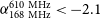 $\alpha_{168\ \text{MHz}}^{610\ \text{MHz}} < -2.1$, making it one of the steepest-spectrum radio halo detected to date, tied with the radio halo in Abell 521 (
 $\alpha_{240\ \text{MHz}}^{610\ \text{MHz}} \approx -2.1$; Brunetti et al., Reference Brunetti2008). Caglar (Reference Caglar2018) investigated the X-ray properties of the cluster, which show both a bi-modal X-ray distribution and a bi-modal optical distribution (Dahle et al., Reference Dahle, Kaiser, Irgens, Lilje and Maddox2002). The cluster is also detected in Planck Sunyaev–Zel’dovich (PSZ) surveys as PSZ2 G175.69 –85.98 (Planck Collaboration et al. 2016a) and is reported to have an SZ-derived mass of
  $5.67^{+0.36}_{-0.40}\times 10^{14}$ M
 $_\odot$. The cluster is reported to have a redshift of
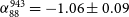
  $0.23$ (Struble & Rood, Reference Struble and Rood1999) where 1 arcmin corresponds to 221 kpc in scale. We show an updated composite image of Abell 141 in Figure 1 with data described in Sections 2.3 and 2.4.

Figure 1. Composite image of Abell 141. Background optical data are from the Pan-STARRS survey, data release 1 (bands r, i, z; Kaiser et al., Reference Kaiser2010; Tonry et al., Reference Tonry2012) with Chandra (blue, Section 2.4) and source-subtracted ASKAP (red, Section 2.3) maps overlaid. The linear scale is at the redshift of the cluster.
1.2. Abell 3404
Abell 3404 was found to host unclassified extended emission permeating the cluster in GaLactic and Extragalactic All-sky MWA (GLEAM; Wayth et al., Reference Wayth2015; Hurley-Walker et al., Reference Hurley-Walker2017) data at 200 MHz from a search for diffuse cluster emission within clusters from the Meta-Catalogue of X-ray detected galaxy Clusters (MCXC; Piffaretti et al., Reference Piffaretti, Arnaud, Pratt, Pointecouteau and Melin2011). Although the emission is elongated, typical of the morphologies of radio relics, its location at the centre of the cluster suggested a halo-type source. The low resolution of the GLEAM data resulted in significant blending of the extended emission with nearby point sources and made it impossible to confirm its nature. Shakouri et al. (Reference Shakouri, Johnston-Hollitt and Pratt2016) investigated the cluster using the Australia Telescope Compact Array (ATCA; Frater et al., Reference Frater, Brooks and Whiteoak1992) as part of the ATCA REXCESSFootnote c Diffuse Emission Survey (ARDES), though they found no evidence of a radio halo or other diffuse radio source. In advance of this publication, Brüggen et al. (Reference Brüggen2021) noted the detection of diffuse emission in Abell 3404 on the edge of a widefield observation of the cluster system Abell 3391-95 but leave the detailed characterisation to this work. The cluster has an SZ-derived mass of  $7.96^{+0.23}_{-0.21}\times 10^{14}$ M
 $_\odot$ and redshift
  $z=0.1644$ (Planck Collaboration et al. 2016a). At the cluster redshift, 1 arcmin corresponds to 170 kpc in scale. A composite image of Abell 3404 is shown in Figure 2.
2. Data & methods
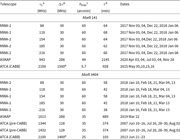
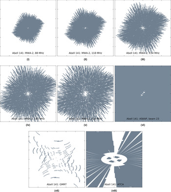
New data presented in this work are described in the following sections. A summary of observations used in this work and described in this section is presented in Table 1. We also provide representative plots of the u–v coverage for all data sets in Appendix, A.
Table 1. Details of the radio observations of Abell 141 and Abell 3404.

a Central observing frequency.
b Observation bandwidth.
c Maximum angular scale observation is sensitive to at the respective central frequency with a u–v limit employed during imaging.
d Total observing time.
e Originally a 2049 MHz band, significant RFI flagging reduces the usable bandwidth.
2.1. MWA-2
2.1.1. Data processing
Both Abell 141 and Abell 3404 were observed with the MWA-2 as part of a follow-up of candidate radio halos and relics detected with the GLEAM survey. The observations covered five frequency bands (of 30-MHz bandwidth): 88, 118, 154, 185, and 216-MHz. Observation details are presented in Table 1. The MWA data are processed following Duchesne et al. (Reference Duchesne, Johnston-Hollitt, Zhu, Wayth and Line2020). Briefly, MWA data are observed in a 2-min snapshot observing mode, with each 2-min snapshot calibrated and imaged independently and stacked in the image plane at the end.
Figure 2. Composite image of Abell 3404. Background optical data are from the SuperCOSMOS Sky Survey (Hambly et al., Reference Hambly2001a b,c). Radio and X-ray data overlaid as in Figure 1. The linear scale is at the redshift of the cluster.
Figure 3. Abell 141 radio maps. (i) ASKAP, 943-MHz image at robust  $=+0.25$. The overlaid contours are as follows: MWA-2, 118-MHz robust
  $=+2.0$ image, single white contour at
  $3\sigma_{\text{rms}}$ (4.7 mJy beam-1); ASKAP, 943-MHz source-subtracted image, solid magenta contours starting from
  $3\sigma_{\text{rms}}$ (
 $\sigma_{\text{rms}} = 0.105$ mJy beam-1), increasing with increments of 2 with a single dotted magenta contour at
  $2\sigma_{\text{rms}}$. Sources subtracted after SED modelling are labelled. (ii) ASKAP, 943-MHz source-subtracted image with contours as follows: MWA-2, 216-MHz robust
  $=0.0$, black contours starting at
  $3\sigma_{\text{rms}}$ (11.4 mJy beam-1); ATCA full-band image at robust
  $=0.0$, magenta contours starting at
  $3\sigma_{\text{rms}}$ (
 $\sigma_{\text{rms}} = 27$
  $\mu$Jy beam-1). For both figures, the resolution of each image is shown in the bottom right corner, with the grey ellipse corresponding to the background map. The linear scale in the top right is at the redshift of the cluster.
We use in-field calibration on a global sky model generated from the GLEAM, NVSS, and SUMSS catalogues (where survey coverage is available) using the Mitchcal algorithm (see Offringa et al., Reference Offringa2016). The calibrated data are then imaged using WSClean (Offringa et al., Reference Offringa2014; Offringa & Smirnov, Reference Offringa and Smirnov2017) to perform amplitude and phase self-calibration before imaging again to a lower threshold (i.e. CLEANing more deeply). After initial primary beam correction using the most recent Full-Embedded Element model (Sokolowski et al., Reference Sokolowski2017), these CLEANed images are then corrected for ionosphere-related astrometric shifts using fits_warp.pyFootnote d (Hurley-Walker & Hancock, Reference Hurley-Walker and Hancock2018) and finally corrected for residual primary beam errors and flux scale errors with flux_warpFootnote e (Duchesne et al., Reference Duchesne, Johnston-Hollitt, Zhu, Wayth and Line2020) to ensure a common flux scaling across snapshots. The snapshots are then co-added, weighted by the square of the primary beam response and local noise.
We make a number of image sets for multiple purposes: (a) using an image weighting with a ‘Briggs’ robustness parameter of 0.0 for a maximum resolution image, (b) robust  $=+2.0$, and (c) robust
  $=+1.0$ with an additional 120 arcsec Gaussian taper applied to produce a more common sensitivity between the five frequencies and to enhance the low surface-brightness emission in individual snapshots further. We find that because of the slight difference in inner u–v sampling between the five frequencies (see Appendix, A, Figures 11(i)–(v) and 12(i)–(v)), the 88- and 118-MHz images do not require additional tapering, though for Abell 3404 we find we can use the robust
  $=+2.0$ images for flux density measurement without additional confusion.
Figure 3(i) and 3(ii) shows the  $3\sigma_{\text{rms}}$ contours of the robust
  $=+2.0$, 118-MHz image and the robust
  $=0.0$, 216-MHz image of Abell 141, respectively. Similarly, Figure 4(i) shows the
  $3\sigma_{\text{rms}}$ contour of the robust
  $=+2.0$, 118-MHz image of Abell 3404, and Figure 4(ii) shows the
  $3\sigma_{\text{rms}}$ contour of the robust
  $=0.0$, 216-MHz image.
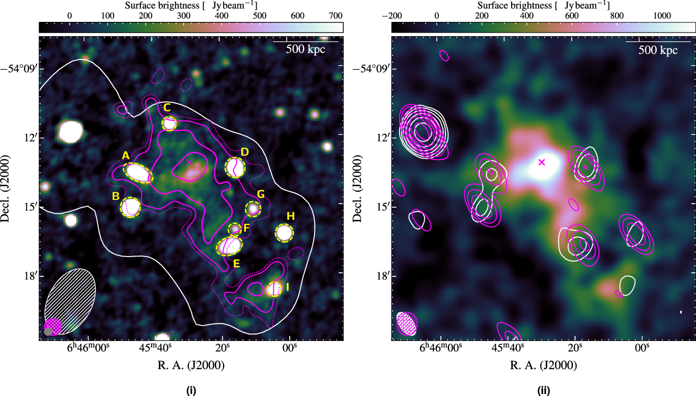
Figure 4. Abell 3404 radio maps. (i) ASKAP, 1013-MHz image at robust  $=+0.5$. The overlaid contours are as follows: MWA-2, 118-MHz robust
  $=+2.0$, single white contour at
  $3\sigma_{\text{rms}}$ (6.1 mJy beam-1); ASKAP, 1013-MHz tapered source-subtracted image, solid magenta contours starting from
  $3\sigma_{\text{rms}}$ (
 $\sigma_{\text{rms}} = 0.84$ mJy beam-1), increasing with increments of 2 with a single dotted magenta contour at
  $2\sigma_{\text{rms}}$. Sources subtracted after SED modelling are labelled. (ii) ASKAP source-subtracted, tapered, with contours as follows: MWA-2, 216-MHz robust
  $=0.0$ image, white contours starting at
  $3\sigma_{\text{rms}}$ (
 $\sigma_{\text{rms}} = 6.6$ mJy beam-1); ATCA, 2.4-GHz robust
  $=0.0$ image, magenta contours starting at
  $3\sigma_{\text{rms}}$ (
 $\sigma_{\text{rms}} = 0.24$ mJy beam-1). The ellipses in the the lower left are as in Figure 3, and the linear scale is at the redshift of the cluster.
2.1.2. Measuring dirty flux density
Snapshot imaging results in residual dirty flux (i.e. emission that has not been deconvolved by the CLEAN algorithm) that becomes significant in final stacked images as the CLEANing depth is set in the individual snapshot images. Using multiscale CLEAN can mitigate this somewhat as the root-mean-square (rms) noise on larger scales allows CLEANing of large structures below the point-source CLEAN depth. The result is measurement of residual dirty flux, which 1) has a point spread function (PSF) that differs from the restoring beam and 2) the dirty flux may be reduced or increased compared to the equivalent CLEAN flux due to complex PSF sidelobe interactions. We assume that the PSF difference is small—i.e. the fitted restoring beam is an accurate representation of the PSF. To test the difference in measured dirty to CLEAN flux density, we simulate 2-D circular Gaussian sources in all snapshots with an arbitrary  $S = 1$ Jy with varying full-width at half maximum (FWHM) sizes, ranging from 5 arcsec to 575 arcsec in 30 arcsec intervals and measure the integrated flux density in the dirty and CLEANed maps. We find that the ratios of measured
  $S_{\text{p,dirty}}/S_{\text{p,CLEAN}}$ (peak) and
  $S_{\text{dirty}}/S_{\text{CLEAN}}$ (integrated) decrease down to
  $\sim$0.5–0.6 for structures up to 10 arcmin for the Abell 3404 data, but increase by only a few per cent for Abell 141. We show the robust
  $=+2.0$ results in Figure 5.
To correct for this, we create separate CLEAN component model and residual stacked images to match the restored stacked image. When measuring S for real sources, we use the restored image to guide the integration region, but sum the CLEAN model and add the integrated residuals with a correction factor applied to the residual flux density determined by the size of the emission region. The correction factor is determined by the convolved source size and estimated from the nearest simulated ratio of  $S_{\text{dirty}}/S_{\text{CLEAN}}$.
2.2. ATCA
Abell 3404 was observed with both the Compact Array Broadband Backend (CABB; Wilson et al., Reference Wilson2011) and the ATCA correlator prior to the CABB installation (hereafter ‘pre-CABB’, Project Codes C1683 and C2837; Johnston-Hollitt et al., Reference Johnston-Hollitt, Finoguenov, Böhringer, Pratt and Croston2007,, Reference Johnston-Hollitt, Basu, Nord, Hindson and Shakouri2013). The observation details are listed in Table 1, though note for both the CABB and pre-CABB observations Abell 3404 was observed in a ‘u–v cuts’ mode at a range of hour-angles, but not filling in the u–v plane significantly. The pre-CABB and CABB data have different phase centres, and the lower end of the CABB data is flagged due to RFI so the two data sets are imaged independently. Abell 141 was observed with the CABB (Project Code C2915; Shimwel et al., Reference Shimwel, Stroe and Hoang2015), though two configurations were used: 1.5C and 6A, with maximum/minimum baselines of 4500/77 and 5939/337 m, respectively.
Calibration for all ATCA data follows standard data reduction procedures using miriad (Sault et al., Reference Sault, Teuben, Wright, Shaw, Payne and Hayes1995). Bandpass and absolute flux calibration is performed using the standard ATCA centremetre calibrator, PKS B1934-638, and appropriate secondary calibrators bracket the source observations, used for complex gain and phase calibration. We perform two rounds of self-calibration on each data set, using WSClean to create initial CLEAN component models and the Common Astronomy Software Applications (CASA; McMullin et al., Reference McMullin, Waters, Schiebel, Young, Golap, Shaw, Hill and Bell2007) task, gaincal, to solve for phase-only gain solutions on successively shorter intervals (i.e. 120 and 30 s). Additionally, final imaging for the Abell 3404 data removes the longest baselines formed with antenna 6 to achieve a more well-behaved point spread function. Imaging for all data sets is otherwise similar, utilising a ‘Briggs’ robustness parameter of 0.0, and splitting the full CABB bands into smaller subbands. Note that significant RFI flagging occurs in the 16-cm band for the ATCA data, and the final usable band for CABB observations is  $\sim\! 1.5$ GHz and is split into subbands of
  $\Delta\nu = 300$ MHz for discrete source measurements.
Figure 3(ii) shows the robust  $=0.0$ full-band 2.2-GHz ATCA map for Abell 141 convolved to 18 arcsec. Figure 3 shows the similar 2.4-GHz full-band map for Abell 3404.
2.3. ASKAP
ASKAP operates between 700 and 1800 MHz and features a Phased Array Feed (PAF; DeBoer et al., Reference DeBoer2009; Hotan et al., Reference Hotan2014; McConnell et al., Reference McConnell2016) allowing the creation of 36 independent primary beams which can be arranged in a number of different footprints to create large  $7^\circ \times 7^\circ$ mosaics in ‘6 by 6’ primary beam footprints. ASKAP has recently been used to complete some observations for early science and survey projects (e.g. the Evolutionary Map of the Universe, EMU; Norris et al., Reference Norris2011). Abell 3404 and Abell 141 feature in early science observations; however, both Abell 141 and Abell 3404 sit towards the edges of primary beams. The ASKAP data are publicly available and are retrieved from the CSIROFootnote f ASKAP Science Data Archive (CASDA; Chapman et al., Reference Chapman, Dempsey, Miller, Heywood, Pritchard, Sangster, Whiting and Dart2017). Prior to being made available through CASDA, the ASKAPsoftFootnote g pipeline uses daily observations of PKS B1934-638 for bandpass calibration, with each of the 36 beams being calibrated independently. Additionally, the data are averaged to 1 MHz/10 s spectral/temporal resolution. The full bandwidth for each observation is 288 MHz. We summarise additional observation details in Table 1.
2.3.1. ASKAP—Abell 3404
The ASKAP Scheduling Block (SB)8275 (Harvey-Smith et al., Reference Harvey-Smith2018) has two overlapping beams containing Abell 3404 (beam 17 and 23) with a central observing frequency of  $\nu_{\text{c}} = 1013.5$ MHz. We follow a similar self-calibration process to the ATCA data described in Section 2.2, though this calibration does not reduce the well-known, but not currently understood artefacts that appear around bright sources at a
  $\sim1\%$ level. For the two beams containing Abell 3404, these artefacts are negligible and do not interfere with the cluster. Imaging is performed using WSClean, and we image by splitting the data into 4 subbands of
  $\Delta\nu = 72$ MHz, jointly CLEANing in the fullband multi-frequency synthesis (MFS) image. Imaging for these data is done by first masking the diffuse emission within the cluster region, ensuring all discrete sources are included in the CLEAN process. The initial image weighting is robust
  $=+0.5$, which we found to be most accurate for modelling the discrete cluster sources. The second image set we produce is the re-imaged residuals convolved with a 25 arcsec beam to highlight diffuse cluster emission. Finally, we re-image the residuals with an additional 35 arcsec taper in 3 subbands of
  $\Delta\nu = 96$ MHz.
For each image set, we linearly mosaic beams 17 and 23, applying a correction for primary beam attenuation assuming a 2-dimensional Gaussian model that scales with  $1.09\lambda/D$ (A. Hotan, priv. comms.) with
  $D=12$ m the diameter of the ASKAP dishes. For quality assurance, we compare the spectral energy distribution (SED) of a nearby, bright test source measured by the MWA-2, ATCA, and additional survey data and find that the ASKAP data follow the expected flux density. Additionally, we find an astrometric offset of
  $\Delta\delta_{\text{J2000}} \sim -0.0055$, which we correct in the image World Coordinate System (WCS) metadata. Figure 4(i) shows the ASKAP full-band robust
  $=+0.5$ image with the source-subtracted 35 arcsec tapered image as contours.
2.3.2. ASKAP–Abell 141
Abell 141 is present on the edge of a beam (23) in a number of ASKAP observationsFootnote h. After an initial round of imaging with all available observations, we find most of the observations contain significant radial artefacts crossing the cluster from a nearby bright source which is unable to be removed via direction-independent calibration. We find the SB12704, SB15191, and SB18925 observations do not show significant artefacts and combine those observations for further joint imaging. We opted to self-calibrate the data, generating a combined, jointly deconvolved model image of the three data sets then self-calibrating each data set individually based on the combined model. Initial imaging was carried out similarly to the Abell 3404 data, masking the cluster diffuse emission. The difference in this imaging process is we use a robust  $=+0.25$ weighting scheme, which for these observations provided a better model of the cluster discrete sources. Additionally, we find that since the diffuse emission is much fainter than in Abell 3404, and because the cluster lies further from the primary beam centre, we only consider the full-band re-imaged residual visibilities rather than the subbands produced while CLEANing. As there is only a single primary beam, mosaicking is not required; however, a primary beam correction is applied. Because the source lies to the edge of the beam, we compare the ASKAP flux densities of sources across the image to extrapolated flux densities derived from the ATCA subband images and the catalogue used for MWA-2 flux scaling (independently, see Duchesne et al., Reference Duchesne, Johnston-Hollitt, Zhu, Wayth and Line2020 for details of the calibration catalogue). For comparison with the MWA catalogue, the data are first convolved to a common resolution. We find the flux densities of sources do not deviate beyond
  $\sim 10$%. We find no discernible astrometric offset for these data.
The full-band, robust  $=+0.25$ image is shown in Figure 3(i) with the source-subtracted, 45 arcsec robust
  $=+0.25$ image as contours in Figure 3(i) and the background in Figure 3(ii).

Figure 5. Comparison of dirty and CLEANed flux densities in the robust  $+2.0$ MWA-2 images as a function of source FWHM for simulated Gaussian sources. Note that individual snapshot
  $S_{\text{dirty}}/S_{\text{CLEAN}}$ ratios are shown as transparent grey lines with the mean value plotted as a solid red line, and a shaded region corresponding to the standard deviation between snapshots.
2.4. Chandra
Both clusters have been observed with the Advanced CDD Imaging Spectrometer (ACIS-I) on the Chandra X-ray observatory. We obtain both data sets (Abell 141: Obs. ID 9410, PI: Smith, 19.91 ks; Abell 3404: Obs. ID 15301, PI: Murray, 9.96 ks) from the Chandra data archive and use the CIAO software suite (v4.12, with CALDBFootnote i v4.9.1; Fruscione et al., Reference Fruscione2006) to process the data following standard Chandra data reduction procedures, using the task chandra_repro to generate the level-2 event file. From this, we generate count and exposure-corrected flux images using the task fluximage applying 1 arcsec binning for the full energy band ([0.5–7] keV). We use wavdetect to identify point-like sources in the images and remove them, finally creating images in the [0.5–2] kev band. For Abell 141, as there is an AGN at the centre of the northern sub-cluster that is subtracted, we fill in the removed component using the task dmfilth. Additional smoothing with a  $\sigma = 6$ arcsec, 2-dimensional Gaussian kernel is applied to the exposure-corrected image, using the task aconvolve. The [0.5–2] kev exposure-corrected, smoothed, and source-subtracted Chandra images are shown in Figure 5 for each cluster.
3. Results and discussion
3.1. Morphology
The ASKAP and MWA-2 data show clear evidence of central diffuse emission and additional extended peripheral structures in Abell 141 and Abell 3404 (see Figures 3(i), 4(i), 6(i), and 6(ii)), not necessarily associated with any particular radio galaxy, though it is unclear if these components are associated with the central diffuse sources. No diffuse radio emission is detected in the ATCA data for either clusters (Figures 3(ii) and 4(ii)). We show the exposure-corrected, smoothed X-ray maps in Figure 6 to highlight the morphology of the clusters and the co-location of the radio emission.

Figure 6. Exposure-corrected, smoothed, point source-subtracted [0.5–2] kev Chandra maps with source-subtracted ASKAP contours overlaid. (i) Abell 141: ASKAP contours as in Figure 3(i), but without the  $2\sigma_{\text{rms}}$ contour. (ii) Abell 3404: ASKAP contours are the source-subtracted without tapering, but convolved with a 25 arcsec beam (hence, slightly higher resolution than the tapered, source-subtracted map). In (i) the yellow, dashed box indicates the peripheral diffuse source. In (ii) we show the regions within which we extract radio and X-ray surface brightness profiles (yellow sectors) and indicate extended radio components in those profiles (yellow, dashed rectangles) that may indicate radio shocks discussed in Section 3.4.3. The magenta lines indicate the edge of the ACIS-I field-of-view.
3.1.1. Abell 141
The central, diffuse radio emission in Abell 141 has a slightly elongated morphology as seen in the source-subtracted ASKAP data, with an extension towards the southeast becoming a distinct peripheral component (yellow, dashed box in Figure 6(i)). The radio emission fills the volume between two X-ray sub-clusters and extends into the northern sub-cluster. Excluding the peripheral source, we measure the size of the central diffuse emission in Abell 141 from N–S and E–W within  $2\sigma_{\text{rms}}$ contours finding deconvolved dimensions of
  $4.2$ and
  $3.7$ arcmin, respectively, corresponding to a linear size of 910 and 790 kpc. We will consider the mean linear extent to be 850 kpc. Additionally, the SE peripheral component has a maximum projected extent of
  $2.6$ arcmin, corresponding to 550 kpc.
3.1.2. Abell 3404
The central diffuse emission in Abell 3404 is also elongated, and we similarly see peripheral extended components that may not be associated with the central diffuse source—these are most prominent in the 25 arcsec source-subtracted ASKAP image (contours in Figure 6(ii), indicated by yellow, dashed rectangles). The peak of the central radio emission is co-located with the X-ray peak, and the radio emission generally fills the X-ray-emitting area. The size of the central diffuse source is measured in the ASKAP source-subtracted, 35 arcsec tapered image within  $2\sigma_{\text{rms}}$ contours as above, finding angular sizes in the N–S and E–W directions of
  $5.3$ arcmin and
  $3.9$ arcmin, respectively, corresponding to linear sizes of 900 and 660 kpc. We note that the the N–S direction is influenced by additional peripheral components, though it is not clear if these are part of the central emission or not (further discussed in Section 3.4.3). For the estimate of the size, the SE component—which is more distinct—is not included. We again will consider the mean linear extent of 770 kpc in the following sections. The NE peripheral component is found to have a maximum projected size of 1.7 arcmin (270 kpc), and the SW component is found to be 1.5 arcmin (230 kpc) in extent.
3.2. Radio spectral properties
3.2.1. Flux densities
Figures 3(i) and 4(i) also show relevant discrete sources that are projected onto the clusters within the MWA-2 emission. For the ASKAP data, these were subtracted in the visibilities using CLEAN component models (Section 2.3), but in the MWA data, their contribution is subtracted from the integrated flux density measurement after extrapolation from their measured SEDs. The central diffuse emission in Abell 3404 from 185 to 216 MHz is only barely detected above a  $3\sigma_{\text{rms}}$ significance in the MWA-2 data, with generally poorer image qualities and lack of detection in individual snapshots. As we cannot guarantee significant enough flux is recovered in these images, we opt not to provide measurements for Abell 3404 in the 185- and 216-MHz MWA-2 images. We instead measure the source using the 200-MHz GLEAM image. For Abell 141, we use all MWA-2 bands and re-measure the source in the 169-MHz EoR-0 image (Offringa et al., Reference Offringa2016) and the 200-MHz GLEAM image. We find the 169-MHz measurement is lower than that reported by Duchesne et al. (Reference Duchesne, Johnston-Hollitt, Offringa, Pratt, Zheng and Dehghan2021b) largely due to additional discrete source-subtraction.
Table 2. Discrete source SED properties for both clusters.

a Frequency range over which source is modelled.
b Fit with a curved power law model.
c Inverted spectrum.
d Source could not be modelled, but is not distinguishable from ‘E’ in MWA data.
e No uncertainty is given as the SED is only over the ASKAP subbands, and we do not quantify the internal flux scale uncertainty across the band.
Table 2 shows the fitted power law properties of the discrete sources in each cluster. We measure the flux density of the peripheral diffuse sources in Abell 141 and Abell 3404 in the full-band, 25 arcsec ASKAP image, though are unable to provide a spectral index estimate. Individual flux density measurements of the diffuse sources are provided in Table 3, indicating the contributions from discrete sources that are subtracted from the total integrated flux density in the process. The peripheral components in each cluster contribute to the diffuse source measurements as we cannot subtract them from the MWA data and we only provide measurements of the perierphal sources in the full-band ASKAP images. Relevant details of images used for flux density measurements are also provided in Table 3.
3.2.2 Diffuse source spectral indices
The central diffuse radio sources can be described by a simple power law between 88 and 943 MHz for Abell 141 and 88 and 1 110 MHz for Abell 3404. Figure 7 plots the measured data as well as the best-fit power law models. The spectral index for the central diffuse source in Abell 3404 ( $\alpha_{88}^{1\,013} = -1.66 \pm 0.07$) pushes it into the ‘ultra-steep spectrum radio halo’ category (defined by
  $\alpha < -1.5$, USSRH; Cassano et al., Reference Cassano2013). We find that the central emission in Abell 141 has a flatter spectrum than reported by Duchesne et al. (Reference Duchesne, Johnston-Hollitt, Offringa, Pratt, Zheng and Dehghan2021b), though this is in part due to the subtraction of three discrete sources with steep spectra. We report all derived source properties in Table 4, including source linear size, spectral index, and extrapolated monochromatic power at 1.4 and 0.15 GHz.
3.2.3. Limits on high-frequency non-detections
To investigate the non-detections in ATCA data, we obtain upper limits by injecting simulated radio halos into the visibility data. We assume an azimuthally averaged brightness distribution described by (Orrú et al., Reference Orrú, Murgia, Feretti, Govoni, Brunetti, Giovannini, Girardi and Setti2007, but see also Murgia et al., Reference Murgia, Govoni, Markevitch, Feretti, Giovannini, Taylor and Carretti2009; Bonafede et al., Reference Bonafede2017), of the form
 \begin{equation} I(r) = I_0 e^{-r/r_e} \quad [\text{Jy}\,\text{arcsec}^{-2}] ,\end{equation}
with  $I_0$ the peak brightness, the e-folding radius
  $r_e = f/R_{\text{H}}$, and
  $R_{\text{H}}$ the radio halo radius. A median value of f is found to be 2.6 by (Bonafede et al., Reference Bonafede2017, based on radio halo samples described by Cassano et al., Reference Cassano, Brunetti, Setti, Govoni and Dolag2007; Murgia et al., Reference Murgia, Govoni, Markevitch, Feretti, Giovannini, Taylor and Carretti2009). For the purpose of determining limits, we use the calibrated GMRT data presented by Venturi et al. (Reference Venturi, Giacintucci, Brunetti, Cassano, Bardelli, Dallacasa and Setti2007); Venturi et al. (Reference Venturi, Giacintucci, Dallacasa, Cassano, Brunetti, Bardelli and Setti2008) of Abell 141, recalculating the limit for consistency with the current method.
Table 3. Flux density measurements and limits of the diffuse sources.

a Average rms noise within the measured source region.
b Confusing source flux that is subtracted from initial measurement based on SEDs reported in Table 1.
c EoR-0 field image (Offringa et al., Reference Offringa2016) as used by Duchesne et al. (Reference Duchesne, Johnston-Hollitt, Offringa, Pratt, Zheng and Dehghan2021b), re-measured with present integration region and source subtraction, including brightness scaling of 0.69.
d Data originally presented by Venturi et al. (Reference Venturi, Giacintucci, Brunetti, Cassano, Bardelli, Dallacasa and Setti2007).
e Limit from mock radio halos as described in Section 3.2.3.
To determine the initial halo brightness and spectrum, we use the brightness from the ASKAP data and spectral index reported in Section 3.2.2. Additionally, we find values of f (Equation (1)) to be 2.0 and 1.9 that recover adequate model flux for the Abell 141 and Abell 3404 radio halos, respectively. We use WSClean to inject the simulated halo as a function of frequency into the relevant data sets. During imaging of the mock radio halo, we increase brightness by factors of  $\sqrt{2}$ until a detection is made. Imaging is done as a two-part process: first, the model data are imaged alone and then imaged with the true calibrated data. The imaging of the model alone allows us to investigate the percentage of flux lost due to the u–v sampling. For Abell 141, we image both the ATCA and GMRT data with a 30 arcsec Gaussian taper applied to the visibilities to maximise the likelihood of detection. We find that the ATCA observation of Abell 141 only recovers
  $\sim\! 20$% of the model radio halo flux due to the lack of inner spacings limiting sensitivity on larger scales, with the GMRT observation recovering
  $\sim\! 60$%. For Abell 3404, the flux recovered is
  $\sim 70$% and
  $\sim 90$% for the pre-CABB and CABB data, respectively. We use the same detection criterion as Bonafede et al. (Reference Bonafede2017):
  $D_{2\sigma_{\text{rms}}}^{\text{mock}} \geq R_{\text{H}}$, where
  $D_{2\sigma_{\text{rms}}}^{\text{mock}}$ is the diameter of the mock radio halo within
  $2\sigma_{\text{rms}}$ contours. As per Bonafede et al. (Reference Bonafede2017), we opt to consider the model radio halo flux density for the limit, as this is the flux density that would be required to make the detection. The resultant limits, along with new limits obtained for the GMRT data (Venturi et al., Reference Venturi, Giacintucci, Brunetti, Cassano, Bardelli, Dallacasa and Setti2007; Venturi et al., Reference Venturi, Giacintucci, Dallacasa, Cassano, Brunetti, Bardelli and Setti2008), are provided in Table 3, though are not used in fitting in Section 3.2.2.
We note that the limit found for the GMRT data of Abell 141 is higher than what is reported by Venturi et al. (Reference Venturi, Giacintucci, Brunetti, Cassano, Bardelli, Dallacasa and Setti2007); Venturi et al. (Reference Venturi, Giacintucci, Dallacasa, Cassano, Brunetti, Bardelli and Setti2008):  $\sim 7$ mJyFootnote j. This discrepancy is a result of, in part, the
  $\sim 60$% of flux lost to u–v sampling, and the difference in the modelled brightness profile, where Venturi et al. use optically thin concentric spheres (see also Brunetti et al., Reference Brunetti, Venturi, Dallacasa, Cassano, Dolag, Giacintucci and Setti2007). The remaining difference may be contributed from a different model geometry and spectrum and a bias that occurs when measuring the integrated flux density of low-SNR extended sources (Stroe et al., Reference Stroe2016, but see also Helfer et al., Reference Helfer, Thornley, Regan, Wong, Sheth, Vogel, Blitz and Bock2003).
Cuciti et al. (Reference Cuciti, Brunetti, van Weeren, Bonafede, Dallacasa, Cassano, Venturi and Kale2018) perform a similar mock halo analysis for GMRT and Karl G. Jansky Very Large Array (JVLA) data to test flux recovery of incomplete u–v sampling. An important note they make is that the recovered flux density fraction decreases as the mock halo brightness decreases. We note that the flux recovery fraction for our mock halos is based on the limits. Appendix, A shows representative u–v coverage plots for the observations used in this work (MWA-2, ASKAP, ATCA, and GMRT). These plots highlight that inner u–v sampling for the GMRT and ATCA (Abell 141) observations is lacking, whereas the MWA-2, ASKAP, and even the pre-CABB and CABB data for Abell 3404 have much more densely sampled inner u–v data. We note, however, that the smaller  $\lambda$ values become less populated towards the higher end of the MWA-2 band. We opt not to provide limits on the MWA-2 data between 185 and 216 MHz for Abell 3404 due to partial detection of the radio halo combined with significant confusion with discrete sources.
3.3. Radio–X-ray correlation
Radio halo brightness ( $I_{\text{R}}$) is often observed to correlate with the X-ray surface brightness (
 $I_{\text{X}}$) of the ICM (
 $I_{\text{R}} \propto {I_{\text{X}}}^k$; Govoni et al., Reference Govoni, Enÿlin, Feretti and Giovannini2001). Radio halos are typically observed with a sub-linear slope (e.g. Giacintucci et al., Reference Giacintucci2005; Rajpurohit et al., Reference Rajpurohit2018; Hoang et al., Reference Hoang2019a; Botteon et al., Reference Botteon2020c; Rajpurohit et al., Reference Rajpurohit2021; Bruno et al., Reference Bruno2021); conversely, mini-halos have been found to have super-linear slopes (Ignesti et al., Reference Ignesti, Brunetti, Gitti and Giacintucci2020). We use the exposure-corrected, source-subtracted, smoothed [0.5–2] kev Chandra data along with the low-resolution, source-subtracted ASKAP images to perform a similar analysis for Abell 141 and Abell 3404.

Figure 7. SEDs of the diffuse emission in Abell 141 and Abell 3404. The lines are power law fits, with 95% confidence intervals represented by the shaded regions. Upper limits are represented by arrows. The fits are extrapolated to ATCA frequencies for ease of comparing to ATCA limits.
Table 4. Derived radio halo properties.

Following a procedure described by Ignesti et al. (Reference Ignesti, Brunetti, Gitti and Giacintucci2020), we construct grids across the diffuse emission with cell sizes corresponding to the ASKAP beam major axis. For Abell 141, this is 49′′, corresponding to 178 kpc and for Abell 3404 this is 44′′, corresponding to 124 kpc. We fit the data as  $\text{log}_{10}(I_{\text{R}}) = k \text{log}_{10}(I_{\text{X}}) + C$ using the BCES methodFootnote k with an orthogonal regression. Figure 8 shows the results for (i) Abell 141 and (ii) Abell 3404. For both, we separate out the contribution from the peripheral components, with each grid shown on the inset for each figure. Abell 3404 shows strong correlation (with Spearman rank-order correlation coefficient,
  $\rho = 0.89$), and we find a sub-linear trend with
  $k = 0.53\pm0.04$. While many halos have been found with
  $k \gtrsim 0.6$ (e.g. Govoni et al., Reference Govoni, Enÿlin, Feretti and Giovannini2001; Botteon et al., Reference Botteon2020c; Rajpurohit et al., Reference Rajpurohit2021), we note the steep-spectrum radio halo in MACS J1149.5
 $+$2223 is found to have
  $k \lesssim 0.6$ (Bruno et al., Reference Bruno2021). The SW peripheral component (blue points, Figure (ii)) appears unassociated, whereas the NE component follows the correlation tightly. For the fit, the NE component is included. For Abell 141, we find no significant correlation (
 $\rho = 0.31$). This may indicate a mixture of emission components, though Shimwell et al. (Reference Shimwell, Brown, Feain, Feretti, Gaensler and Lage2014) notes, in reference to the Bullet Cluster radio halo showing a similar lack of correlation, this may be due to the halo occurring during a specific stage of a complex merger.
3.4. Cluster dynamics and source classification
3.4.1. Abell 141—pre-merger?
The dynamic nature of Abell 141 has been studied extensively by (Dahle et al., Reference Dahle, Kaiser, Irgens, Lilje and Maddox2002, in optical) and (Caglar, Reference Caglar2018, hereafter C18, in X-ray). Dahle et al. (Reference Dahle, Kaiser, Irgens, Lilje and Maddox2002) and C18 find that the bi-modal distribution (as seen in the X-ray in Figure 6(i)) represents two subclusters (labelled A141N and A141S by C18) which have not completed a core-crossing—i.e., the cluster is likely in a pre-merging state. C18 reports that X-ray-emitting gas between the two subclusters features a hotspot, which may imply the presence of a shock or shocks. We note that the central diffuse radio emission coincides more with the A141N subcluster but extends into the region between the subclusters. Most radio halos have been detected in clusters that are in a merging or dynamic state (see e.g. Cassano et al., Reference Cassano2013), with three examples in the literature of likely pre-merger subclusters: Abell 399–401 (Murgia et al., Reference Murgia, Govoni, Feretti and Giovannini2010), MACS J0416.1 –2403 (Ogrean et al., Reference Ogrean2015), and Abell 1758N–S (Botteon et al., Reference Botteon2018). We note in the cases of Abell 399–401 and Abell 1758N–S, each subcluster in the corresponding mergers clearly host their own radio halos, whereas we do not detect two distinct radio halos in the A141N and A141S subclusters. The emission may represent a bridge between the subclusters rather than a traditional giant radio halo (see Govoni et al., Reference Govoni2019; Botteon et al., Reference Botteon2020a; Hoeft et al., Reference Hoeft2020; Bonafede et al., Reference Bonafede2021), though due to the resolution of our data, we cannot confirm bridge emission distinct from the radio emission that permeates A141N.

Figure 8. Radio–X-ray point-to-point correlation for (i) Abell 141 and (ii) Abell 3404. Upper limits correspond to cells where  $I_{\text{R}} < 2\sigma_{\text{rms}}$. The black, dashed line is the best-fitting line with a 95% confidence interval shaded in cyan. The insets show the Chandra X-ray maps with the source-subtracted ASKAP image overlaid as contours as in Figures 6(i) and 4(i) for Abell 141 and Abell 3404, respectively. The cyan boxes on the insets show the cells within which surface brightesses are calculated, and the red and blue cells indicate the locations of the peripheral components.
A radio relic? Some radio relics have been found to be co-located with shocks detected via X-ray emission (e.g. Bourdin et al., Reference Bourdin, Mazzotta, Markevitch, Giacintucci and Brunetti2013; Akamatsu et al., Reference Akamatsu2015; Eckert et al., Reference Eckert, Jauzac, Vazza, Owers, Kneib, Tchernin, Intema and Knowles2016; Di Gennaro et al., Reference Di Gennaro2019). Assuming the central region temperature jump in the X-ray corresponds to a shock, C18 derives a Mach number of  $\mathcal{M}_{\text{X}} = 1.69^{+0.41}_{-0.37}$. If we consider that a radio shock traces the same shock structure and that DSA on a pool of thermal electrons triggers the emission (see e.g. Blandford & Eichler, Reference Blandford and Eichler1987), a corresponding radio Mach number can be calculated from
 \begin{equation} \mathcal{M}_{\text{R}} = \sqrt{\dfrac{2\alpha_{\text{inj}} - 3}{2\alpha_{\text{inj}} + 1}} \, ,\end{equation}
assuming that  $\alpha = \alpha_{\text{inj}} - 0.5$, with
  $\alpha_{\text{inj}}$ the synchrotron injection spectrum index. We find
  $\mathcal{M}_{\text{R}} = 5.9 \pm 0.9$, inconsistent with the X-ray-derived Mach number. This does not necessarily rule out the possibility of the source being a radio shock, as discussed by van Weeren et al. (Reference van Weeren2016); van Weeren et al. (Reference van Weeren2017) (but see also Hoang et al., Reference Hoang2019b; Lee et al., Reference Lee, Jee, Kang, Ryu, Kimm and Brüggen2020), a discrepancy in Mach numbers may indicate that the thermal pool electrons are not seed electrons for the emission—i.e., pre-accelerated fossil electrons may be accelerated by the DSA process. In this case, the injection spectrum may resemble the observed emission spectrum (van Weeren et al., Reference van Weeren2016) with
  $\alpha = \alpha_{\text{inj}}$ and
  $\mathcal{M}_{\text{R}} = 2.1 \pm 0.2$, in agreement with
  $\mathcal{M}_{\text{X}}$. Assuming seed electrons for radio relics originates as fossil electrons rather than thermal pool electrons also alleviates the acceleration efficiency problem for some relics with X-ray-detected shocks (see Botteon et al., Reference Botteon, Brunetti, Ryu and Roh2020b, and references therein). Additionally, simulations show radio galaxies in cluster environments can supply fossil electrons for re-acceleration (Vazza et al., Reference Vazza, Wittor, Brunetti and Brüggen2021). A difference in Mach number may also arise from the X-ray and radio emission preferentially tracing different shocks along a line of sight (see e.g. van Weeren et al., Reference van Weeren2016; Rajpurohit et al., Reference Rajpurohit2020, and references therein) or may arise due to turbulence near the shock front (Domínguez-Fernández et al., Reference Domínguez-Fernández, Bruggen, Vazza, Banda-Barragan, Rajpurohit, Mignone, Mukherjee and Vaidya2021).
The present data (including lack of polarimetry) do not allow us to rule out a radio relic or radio bridge interpretation, or a combination thereof. We consider the source a radio halo because the observed physical characteristics—including its morphology, location, and SED—are consistent with a radio halo classification.

Figure 9. Radio and background-subtracted X-ray surface brightness profile for sectors shown in Figure 6(ii) for Abell 3404. The radio ordinate clips at  $2\sigma_{\text{rms}}$. The dashed-red vertical line is at location of the discontinuity in the northern profile.
3.4.2. Abell 3404—dynamics
Figure 6(ii) shows the exposure-corrected, smoothed, and point-source subtracted [0.5–2] kev Chandra map for Abell 3404, where the X-ray emission is slightly elongated. We note that using XMM-Newton data, Pratt et al. (Reference Pratt, Croston, Arnaud and Böhringer2009) consider the cluster as non-cool core but also not morphologically disturbed based on its centroid shift, w (Poole et al., Reference Poole, Fardal, Babul, McCarthy, Quinn and Wadsley2006, but see also Mohr et al., Reference Mohr, Fabricant and Geller1993), which gives an indication of the dynamic state of the cluster. We repeat the calculation for the present Chandra data, using proffitFootnote l (Eckert et al., Reference Eckert, Molendi and Paltani2011), subtracting a fitted background of  $I_{\text{B}} = (1.41 \pm 0.05) \times 10^{-5}$ ph cm-2 s-1 arcmin-2, finding
  $w = 0.039$ within
  $R_{500} = 1\,280$ kpc (Pratt et al., Reference Pratt, Croston, Arnaud and Böhringer2009), smaller than the expected
  $w > 0.075$ for a disturbed system of this radius. We note that the radio halo detected in Abell S1063 (Xie et al., Reference Xie2020) is similarly detected in a cluster that is considered morphologically relaxed based on this definition.
We also calculate the concentration parameter,  $c_{100/500}$ (and
  $c_{40/400}$; Santos et al., Reference Santos, Rosati, Tozzi, Böhringer, Ettori and Bignamini2008), defined via
 \begin{equation} c_{r_1/r_2} = \dfrac{I_{\text{X}}\left( r < r_1\ \text{kpc}\right)}{I_{\text{X}}\left( r < r_2\ \text{kpc}\right)} \, ,\end{equation}
with  $I_{\text{X}}$ the X-ray surface brightness. We find
  $c_{100/500} = 0.24$ which, in combination with the centroid shift within 500 kpc (
 $w_{500\ \text{kpc}} = 0.039$), places the cluster just outside of the halo-hosting quadrant of the
  $c_{100/500}$–
 $w_{500\ \text{kpc}}$ plane shown by Cassano et al. (Reference Cassano, Ettori, Giacintucci, Brunetti, Markevitch, Venturi and Gitti2010)—no halos appear in clusters with
  $c_{100/500} > 0.2$. We also find
  $c_{40/400} = 0.062$, consistent with non-cool–core clusters (Santos et al., Reference Santos, Rosati, Tozzi, Böhringer, Ettori and Bignamini2008). The ambiguity of the X-ray morphological parameters points towards a low-energy/weak merger or a late stage in the merger. For example, a merger between low velocity subclusters or a high mass-ratio between subclusters may result in low-energy mergers. Given the cluster’s SZ-derived mass of
  $7.96_{-0.21}^{+0.23}\times 10^{14}\ \text{M}_\odot$ (Planck Collaboration et al. 2016b), we can infer the presence of a massive subcluster prior to the merger. Such scenarios are expected to generate USSRHs (Brunetti et al., Reference Brunetti2008) as observed here.
3.4.3. Abell 3404—radio and X-ray shocks?
Figure 6(ii) shows two extended diffuse emission regions (indicated with dashed, yellow rectangles) either side of the cluster center. We do not have sufficient fidelity in the ASKAP subband data to investigate the spectral properties or to remove the northern component from the radio halo measurement, though for the purpose of this section, we consider the possibility that the two extended structures represent radio shocks.
We investigate that possibility by extracting X-ray and radio surface brightness (SB) profiles along the directions of the relic-like sources (extracted regions shown as yellow sectors in Figure 6(ii)). For the X-ray data, we use proffit, masking the point sources indicated in Figure 6(ii) with yellow circles. The X-ray SB profiles are binned ensuring each bin is  $\geq 10\sigma$ and
  $\geq 7\sigma$ for the north and south profiles, respectively. The radio SB profile is extracted using in-house python code fluxtools.pyFootnote m. The extracted profiles in each direction are shown in Figure 8. We find candidate discontinuities in the X-ray SB profile. We fit standard broken power law models, representing an electron density discontinuity either side of a putative shock (see e.g. Owers et al., Reference Owers, Nulsen, Couch, Markevitch and Poole2009; Eckert et al., Reference Eckert, Jauzac, Vazza, Owers, Kneib, Tchernin, Intema and Knowles2016):
 \begin{equation}\rho(r) =\begin{cases}Cr^{-\Gamma_{\text{in}}} , & \text{if } r<r_{\text{break}} \\[3pt] C\dfrac{n_{\text{out}}}{n_{\text{in}}} r^{-\Gamma_{\text{out}}} , & \text{otherwise}\end{cases} ,\end{equation}
with  $\Gamma$ the power law indices either side of the discontinuity,
  $j=n_{\text{out}}/n_{\text{in}}$ the density jump, and C a normalisation factor, and the SB profile is
  $\rho(r)$ integrated along the line of sight. For the southern profile, we find
  $j_{\text{south}} \sim 1$, indicating no evidence for a discontinuity. For the northern profile, we obtain
  $j_{\text{north}} = 1.11^{+0.09}_{-0.10}$. The radio source occurs
  $\sim1$ arcmin (
 $\sim170$ kpc) from the X-ray discontinuity; in the case of a relic associated with a shock, the observed discontinuity in the X-ray profile occurs directly after the relic source (and a hard edge may be seen in the radio map); therefore, the northern peripheral radio source is unlikely to be a relic associated with a shock.
3.5.
Radio halo  $\textbf{\textit{P}}_{\boldsymbol\nu}$–$\textbf{\textit{M}}_{\textbf{500}}$ scaling relations


Despite a somewhat atypical X-ray morphology of each cluster, based on the available data, we classify both central diffuse radio sources as giant radio halos (for Abell 141, consistent with the classification from Duchesne et al., Reference Duchesne, Johnston-Hollitt, Offringa, Pratt, Zheng and Dehghan2021b). Both Abell 141 and Abell 3404 have similar masses, and their constituent radio halos have similar sizes and brightness at  $\sim\! 1$ GHz; however, due to the difference in their SEDs, their 1.4- and 0.15-GHz monochromatic luminosities differ by around a factor of two.
Scaling relationships between radio halo power and various (related) cluster properties have been found (see e.g. Liang et al., Reference Liang, Hunstead, Birkinshaw and Andreani2000; Brunetti et al., Reference Brunetti, Venturi, Dallacasa, Cassano, Dolag, Giacintucci and Setti2007; Basu, Reference Basu2012), somewhat explained physically by turbulent (re-)acceleration models for halo formation (Cassano et al., Reference Cassano2013, hereafter C13). A key finding by (Brunetti et al., Reference Brunetti, Cassano, Dolag and Setti2009, but see also Cassano et al., Reference Cassano, Ettori, Giacintucci, Brunetti, Markevitch, Venturi and Gitti2010; Cassano et al., Reference Cassano2013) is the bi-modality to the sample of halo-hosting clusters, where morphologically disturbed (i.e., likely merging) clusters host radio halos, and most relaxed, X-ray–luminous, and massive clusters without halos have upper limits to radio halo power well below the empirical scaling relations.
Recent updates to the power–mass ( $P_\nu$–
 $M_{500}$) relation (Cassano et al., Reference Cassano2013; Martinez Aviles et al., Reference Martinez Aviles2016; Duchesne et al., Reference Duchesne, Johnston-Hollitt, Offringa, Pratt, Zheng and Dehghan2021b; van Weeren et al., Reference van Weeren2020; Cuciti et al., Reference Cuciti2021) find results largely consistent within reported uncertainties. We update this relation at
  $\nu=1.4$ GHz and
  $\nu=0.15$ GHz following (van Weeren et al., Reference van Weeren2020, hereafter vW20). For this work, we incorporate the compiled literature sample of halos reported by C13 and Martinez Aviles et al. (Reference Martinez Aviles2016), halos in Abell S1121 and Abell 2811 reported by Duchesne et al. (Reference Duchesne, Johnston-Hollitt, Offringa, Pratt, Zheng and Dehghan2021b), and new halos reported in the literature from 2017 (Parekh et al., Reference Parekh, Dwarakanath, Kale and Intema2017; Wilber et al., Reference Wilber2018; Cassano et al., Reference Cassano2019; Brzan et al. 2019; Xie et al., Reference Xie2020; HyeongHan et al., Reference HyeongHan2020; Giovannini et al., Reference Giovannini2020; Wilber et al., Reference Wilber, Johnston-Hollitt, Duchesne, Tasse, Akamatsu, Intema and Hodgson2020; Hoeft et al., Reference Hoeft2020; Hoang et al., Reference Hoang2021; Di Gennaro et al., Reference Di Gennaro2020; van Weeren et al., Reference van Weeren2020; Raja et al., Reference Raja2020; Knowles et al., Reference Knowles2021; Raja et al., Reference Raja, Rahaman, Datta, van Weeren, Intema and Paul2021), with the exception of the halo in ACT-CL J0528.8 –3927 reported by Knowles et al. (Reference Knowles2021) as its small size and coincidence with a radio-bright BCG suggests a mini-halo. For consistency, cluster masses are obtained from PSZ measurements where available (Planck Collaboration et al. 2016c, with some masses obtained from the South Pole Telescope; Song et al., Reference Song2012; Reichardt et al., Reference Reichardt2013), and only clusters with an SZ-derived mass are used. Note all radio halos are scaled to 1.4 and 0.15 GHz with either a measured spectral index or using the full sample mean,
  $\langle\alpha\rangle = {-1.4\pm0.2}$, following
 \begin{equation} P_{\nu_1} = \dfrac{4 \pi D_{\text{L}}(z)^2}{\left( 1+z\right)^{1+\alpha}} S_{\nu_{\text{obs}}} \left(\dfrac{\nu_1}{\nu_{\text{obs}}}\right)^\alpha \quad [\text{W}\,\text{Hz}^{-1}] \, ,\end{equation}
where  $\nu_{\text{obs}}$ is the closest observed frequency,
  $\nu_1 \in \{0.15, 1.4\}$, and
  $D_{\text{L}}$ is the luminosity distance of the cluster. We do not distinguish between normal giant radio halos and ultra-steep spectrum radio halos defined by
  $\alpha < -1.5$ (USSRH) (e.g. Brunetti et al., Reference Brunetti2008; C13). We note that integrated flux densities measured by vW20 are integrated from a fitted exponential profile (Equation 1) rather than measured directly from the maps and may be generally larger than those measured via integration directly from the pixel sum, especially for low-SNR halos.
We fit the radio halo sample assuming a scaling relation at  $\nu=1.4$ GHz and
  $\nu=0.15$ GHz with a function of the form
  $\log_{\text{10}}(P_{\nu}) = B\times \log_{\text{10}}(M_{500}) + A$ using the BCES method with an orthogonal regression. For comparison with C13 and vW20, we shift their fitted relations to the relevant frequencies via
 \begin{equation} \log_{10}(P_{\nu_1}) = B\log_{10}(M_{500}) + A - \langle \alpha \rangle \log_{10}\left(\dfrac{\nu_2}{\nu_1}\right) \, ,\end{equation}
where  $\nu_2$ is the frequency at which the original scaling relation is fit and with
  $P_{\nu_1} = P_{\nu_2}(\nu_1 / \nu_2)^{\langle \alpha \rangle}$. Figure 10 shows the
  $P_{1.4}$–
 $M_{500}$ (10(i)) and
  $P_{0.15}$–
 $M_{500}$ (10(ii)) planes with the relevant fits and aforementioned data. Best-fit values for the scaling relation for various methods are shown in Table 5 for comparison with other works.

Figure 10. Radio halo  $P_{\text{1.4}}$–
 $M_{\text{500}}$ relation (i) and
  $P_{\text{0.15}}$–
 $M_{\text{500}}$ relation (ii) with best-fitting orthogonal relations from (a) Cassano et al. (Reference Cassano2013) (solid, black), (b) van Weeren et al. (Reference van Weeren2020) (dashed, black), and (c) this work (dotted, black). Halos are taken from the literature (as discussed in Section 3.5) with the addition of the halo in Abell 3404 (blue, upright triangle) and the updated values for Abell 141 (red, downward triangle), for a total of 86 halos. The shaded regions are 99.7% confidence intervals for fits from this work.
Table 5. Fitted values for the  $P_\nu$–
 $M_{500}$ scaling relations for various methods.

The updated position of the radio halo in Abell 141 on both the  $P_{1.4}$–
 $M_{500}$ and
  $P_{0.15}$–
 $M_{500}$ planes is in agreement with the fitted relations, and the halo in Abell 3404 lies below the
  $P_{1.4}$–
 $M_{500}$ relation consistent with the general population of USSRHs (Cassano et al., Reference Cassano2013; Cuciti et al., Reference Cuciti2021) but is closer to the fitted
  $P_{0.15}$–
 $M_{500}$ relation. We note also that if the halo in Abell 141 was only associated with the A141N subclusterFootnote n the halo’s position on both
  $P_\nu$–
 $M_{500}$ relations would be significantly above the best-fitting lines. With a sample size of 86, we find (orthogonal) scaling relations consistent with C13 and vW20 at both frequencies within respective uncertainties but note some deviation from the fit reported by vW20 at 0.15 GHz. Naturally, scaling radio halo powers to frequencies beyond which they are measured introduces additional uncertainties. We also find that the
  $P_\nu | M_{500}$ fittingFootnote o is the most consistent method (albeit shallower than for orthogonal), with results from vW20 (
 $B = 3.84 \pm 0.69$) and Cuciti et al. (Reference Cuciti2021) (
 $B = 3.26 \pm 0.74$ for their ‘statistical’ sample with USSRHs) with both vW20 and Cuciti et al. (Reference Cuciti2021) employing smaller, specific samples.
C13 finds that inclusion of USSRHs steepens the scaling relation at 1.4 GHz, and vW20 finds generally steeper relations at 0.15 GHz for radio halos detected around 0.15 GHz (and presumably generally steeper in spectrum). In Equation 6, we re-scale the scaling relation with an assumed mean  $\langle\alpha\rangle$, where real observations at lower of higher frequencies may bias the sample selection towards steeper or flatter spectrum sources, respectively, finding opposed slopes to the
  $P_\nu$–
 $M_{500}$ relation. Uncertainties are still too significant to confirm this as discussed by vW20.
The concordance between these results and those in the recent literature demonstrates that we are now reaching sufficient sample sizes to have confidence in the scaling relation values. While it has recently been suggested there is little evolution of magnetic field strength as a function of redshift in galaxy clusters and hence a redshift dependence in the power-mass scaling relations are not expected (Di Gennaro et al., Reference Di Gennaro2020), an outstanding question remains regarding if there is a difference in the relations for halos and USSRHs which may be expected from differences in their underlying physics. Yet larger samples of halos, expected in the near future, will allow this to be probed.
4. Summary
We have confirmed the detection of centrally located diffuse, steep-spectrum cluster radio emission in Abell 141, and ultra-steep spectrum emission in Abell 3404. We have presented new observations from the MWA-2, ASKAP, and ATCA of the clusters, with the central diffuse sources detected with the MWA-2 and ASKAP. We conclude that these central diffuse radio sources can be described as giant radio halos with linear extents of  $\sim 850$ and
  $\sim 770$ kpc, for Abell 141 and Abell 3404, respectively. We find that each source has an SED that can be fitted with a normal power law model, with spectral indices of
  $\alpha_{88}^{943} = -1.06 \pm 0.09$ and
  $\alpha_{88}^{1110} = -1.66 \pm 0.07$ for Abell 141 and Abell 3404, respectively, making the radio halo in Abell 3404 the first reported USSRH detected with ASKAP. We find no evidence of these sources in pre-CABB and CABB ATCA data, though find the u–v coverage for the observations preclude detection of the radio halos assuming an exponential brightness profile described by the derived spectral index and the measured size and peak brightness in the ASKAP images. Additional peripheral components are detected along with the main central halos, though only for the SW peripheral source in Abell 3404 do we confirm this is not associated with the central halo. No shocks are detected at the locations of the peripheral components in Abell 3404, and they are unlikely to be relics. These peripheral components may be background/foreground radio galaxies, phoenices, or other extended sources, and we do not classify them here.
We discuss the morphological properties of the two clusters based on their X-ray emission using Chandra data, noting that Abell 141 has previously been found to likely be in a pre-merging state, prior to core passage of the subclusters. Conversely, we find that the dynamic status of Abell 3404 is likely to be in more relaxed state, either in the late stage of a merger or a low-energy merger. The radio–X-ray surface brightness correlation is explored for each cluster, finding strong correlation for Abell 3404 but no significant correlation for Abell 141. Some of these properties make them atypical for most radio-halo-hosting clusters, though we find that the radio halos are located in the expected places on the P–M scaling relations at both 1.4 and 0.15 GHz, given their respective spectral properties and cluster masses (considering Abell 141 a single cluster system). We fit the  $P_{1.4}$–
 $M_{500}$ and
  $P_{0.15}$–
 $M_{500}$ scaling relations with the current sample of radio halos, finding results consistent with the literature suggesting that we are now converging with a high precision on these relations.
Acknowledgements
We thank T. Venturi for providing the calibrated GMRT data set of Abell 141. We also thank the anonymous referee for providing valuable feedback and their suggestion to explore the radio–X-ray surface brightness correlation. SWD acknowledges an Australian Government Research Training Program scholarship administered through Curtin University. The Australian SKA Pathfinder is part of the Australia Telescope National Facility which is managed by CSIRO. Operation of ASKAP is funded by the Australian Government with support from the National Collaborative Research Infrastructure Strategy. ASKAP uses the resources of the Pawsey Supercomputing Centre. Establishment of ASKAP, the Murchison Radio-astronomy Observatory, and the Pawsey Supercomputing Centre are initiatives of the Australian Government, with support from the Government of Western Australia and the Science and Industry Endowment Fund. Support for the operation of the MWA is provided by the Australian Government (NCRIS), under a contract to Curtin University administered by Astronomy Australia Limited. We acknowledge the Pawsey Supercomputing Centre which is supported by the Western Australian and Australian Governments. This paper includes archived data obtained through the Australia Telescope Online Archive (http://atoa.atnf.csiro.au/). This research has made use of data obtained from the Chandra Data Archive and the Chandra Source Catalog, and software provided by the Chandra X-ray Center (CXC) in the application package CIAO. This research has made use of the NASA/IPAC Extragalactic Database (NED), which is operated by the Jet Propulsion Laboratory, California Institute of Technology, under contract with the National Aeronautics and Space Administration. This research made use of a number of python packages not explicitly mentioned in the main text: aplpy (Robitaille & Bressert, Reference Robitaille and Bressert2012), astropy (Astropy Collaboration et al. 2013; Price-Whelan et al., Reference Price-Whelan2018), matplotlib (Hunter, Reference Hunter2007), numpy (van der Walt et al., Reference van der Walt, Colbert and Varoquaux2011), and scipy (Jones et al., Reference Jones, Oliphant and Peterson2001).
Appendix A u–v coverage plots
Figure 11(i)–11(viii) shows u–v coverage (in  $\lambda$, from
  $-3000\lambda$–
 $3000\lambda$) for the Abell 141 data used in this work, excluding MWA-1 data. Similarly, Figure 12(i)–12(ix) shows the u–v coverage for observations of Abell 3404. We include these plots to highlight the coverage offered by both the MWA and ASKAP in comparison to ATCA and GMRT.

Figure 11. u–v coverage plots for Abell 141 data. Axes are centered on zero and range from  $-3000\lambda$ to
  $3000\lambda$. Note that the MWA-2 data are of single 2-min snapshots, representative of the snapshot observations. The true u–v coverage is slightly more filled in. The observation used for the ASKAP example is SB15191.

Figure 12. u–v coverage plots for Abell 3404 data. Axes are centered on zero and range from  $-3000\lambda$ to
  $3000\lambda$.