Simulating Subject Communities in Case Law Citation Networks
 Jerrold Soh Tsin Howe
- Yong Pung How School of Law, Singapore Management University, Singapore, Singapore
We propose and evaluate generative models for case law citation networks that account for legal authority, subject relevance, and time decay. Since Common Law systems rely heavily on citations to precedent, case law citation networks present a special type of citation graph which existing models do not adequately reproduce. We describe a general framework for simulating node and edge generation processes in such networks, including a procedure for simulating case subjects, and experiment with four methods of modelling subject relevance: using subject similarity as linear features, as fitness coefficients, constraining the citable graph by subject, and computing subject-sensitive PageRank scores. Model properties are studied by simulation and compared against existing baselines. Promising approaches are then benchmarked against empirical networks from the United States and Singapore Supreme Courts. Our models better approximate the structural properties of both benchmarks, particularly in terms of subject structure. We show that differences in the approach for modelling subject relevance, as well as for normalizing attachment probabilities, produce significantly different network structures. Overall, using subject similarities as fitness coefficients in a sum-normalized attachment model provides the best approximation to both benchmarks. Our results shed light on the mechanics of legal citations as well as the community structure of case law citation networks. Researchers may use our models to simulate case law networks for other inquiries in legal network science.
1 Introduction
Citations between cases form the bedrock of Common Law reasoning, organizing the law into directed graphs ripe for network analysis. A growing number of complexity theorists and legal scholars have sought to exploit legal networks to uncover insights about complex systems in general and legal systems in particular. Clough et al. [1] show that transitive reduction produces different effects on a citation network of judgments from the United States Supreme Court (“USSC”) as compared to academic paper and patent networks. Fowler et al. [2, 3] pioneered using centrality analysis to quantify the authority of USSC precedent. This inquiry has been since been extended and applied to other courts [4] such as the Court of Justice of the European Union [5], the European Court of Human Rights [6], and the Singapore Court of Appeal (“SGCA”) [7]. Examining case law citation networks (“CLCN”s) from the Supreme Courts of the United States, Canada, and India, Whalen et al. [8] find that cases whose citations have low average ages, but high variance within those ages are significantly more likely to later become highly influential. Beyond case law networks, Bommarito, Katz, and colleagues [9–11] have exploited the network structure of US and German legislation to study the growth of legal systems as well as the law’s influence on society.
The community structure of CLCNs has received significantly less attention. This, however, is a rich area of research that retraces to seminal works in network science [12, 13]. Understanding communities broadly as connected subgraphs with denser within-set connectivity than without [14] allows us to automatically uncover network communities by iteratively removing links between otherwise dense subgraphs [13] or stochastically modelling link probabilities [15, 16]. A wide range of community detection techniques [17–21] as well as measures for evaluating community quality [22–24] have been studied. To our knowledge, two prior works have examined community structures in case law. Bommarito et al. [25] develop a distance measure for citation networks which they exploit to uncover communities in USSC judgments. Mirshahvalad and colleagues [26] use a network of European Court of Justice judgments to empirically benchmark a proposed method for identifying the significance of detected communities through random link perturbation.
Studying community structures in CLCNs can reveal deeper insights for both legal studies and network science. For legal studies, how far communities in CLCNs mirror legal doctrinal areas (e.g., torts and contracts) is telling of judicial (citation) practices. A judge who cites solely on doctrinal considerations should generate likewise doctrinal communities; one who cites for other (legal or political) reasons would transmit noisier signals. Community detection algorithms could also further the task of legal topic classification. Thus far, this has primarily been studied from a text-classification approach [27, 28].
For network science, CLCNs present a special case of the citation networks that have been studied extensively by the field. Studies mapping scientific papers as complex networks have demonstrated that they exhibit classic scale-free degree distributions [29] (but cf [30]). This has been attributed to preferential attachment, in that papers which have been cited more will be cited more. Other factors shaping paper citations include age [31] and text similarity [32]. These variables’ interacting influences on citation formation yield rich structural dynamics in citation networks. For instance, over time, some papers come to be entrenched as central graph nodes while others fade into obsolescence, showing that age alone does not determine centrality [33]. Numerous generative models, discussed further in Part 2.2, have thus been proposed for citation networks, including for web hyperlinks [33–35].
As [1]’s findings suggest, however, the structure of CLCNs may differ from those of these traditional citation networks. In law, judges must consider the authority and relevance of precedent, amongst other things, when citing cases in their judgments. The doctrine of precedent further requires them to prefer certain citations to others. It is thus worth studying how CLCNs relate to traditional citation networks.
To this end, we examine how far generative models proposed for traditional citation networks can successfully replicate CLCNs. After a brief review of existing models (Section 2.2), we propose and evaluate a CLCN-tailored model that attempts to account for the unique mechanics of legal citations. The model is premised on an attachment function that attempts to capture aspects of legal authority, subject relevance, and time decay (Section 2.3). As measures for legal authority and decay are well-established, we focus on how subject relevance may be modelled. We devise a method for simulating node-level subjects and experiment with alternative attachment functions that incorporate these vectors in four different ways: using subject cosine similarity as a standalone linear feature in the attachment model; using the same as fitness coefficients [36]; constraining nodes to citing within subject-conditional “local worlds” [37]; using subjects to generate subject-sensitive PageRank scores [38] (Section 2.3.3). We then study by simulation the topological and community properties of networks produced by these alternative models (Section 3.1) and benchmark promising models (and baselines) against two empirical CLCNs: early decisions of the United States Supreme Court and of the Singapore Court of Appeal (Section 3.2).1
We find that using subject similarity scores as fitness coefficients within a sum-normalized probability function best approximates these actual networks. However, key differences remain between the simulated and actual networks, suggesting that other factors influencing legal citations are remain unaccounted for. Nonetheless, our work represents a first step towards better capturing and studying the mechanics of case law citation networks.
2 Materials and Methods
Section 2.1 sets the legal theory and context behind case law citation formation. Section 2.2 explores how far these are captured by existing models. Section 2.3 explains our proposed models. Section 2.4 describes the simulation protocol. Section 2.5 explains the graph metrics used to evaluate the simulations. Section 2.6 details the benchmark datasets.
2.1 Legal Context
We define a CLCN as a graph
Like all citation networks, CLCNs are time-directed and acyclic.3 CLCNs are unique, however, because the probability that a new node
1. Acknowledge priority or influence of prior art
2. Provide bibliographic or substantive information
3. Focus disagreements
4. Appeal to authority
5. Reinforce the prestige of one’s own or another’s work
Reason (4) is particularly pertinent to case citations in Common Law systems characterized by the doctrine of binding precedent. The doctrine, in brief, means propositions of law central to a court’s essential holding are taken as binding law for future purposes. Lower courts are bound to follow these holdings. While courts at the same level of hierarchy are not technically bound the same way, great deference is generally accorded to past cases nonetheless.
Recent studies have thus sought to measure legal authority with network centrality measures calibrated for the legal domain [2, 3]. Beyond citation counts, a judgment’s authority is further shaped by its subject areas and time context [40]. Lawyers do not think of judgments as simply authoritative in the abstract, but within a given doctrinal subject area (i.e., torts or contracts) and at a given time. Precedential value waxes and wanes as a judgment gets entrenched by subsequent citations, ages into obsolescence over time, and as other complementary or substitute judgments emerge [7, 39]. Relevance, authority, and age are thus key, interconnected drivers of CLCN link formation [8].
2.2 Existing Models
How far are these legal mechanics captured by existing network models? In this section, we review existing citation network generative models and consider how they may be used to simulate CLCNs. Note that this paper is not a comprehensive review and will only highlight illustrative examples.
2.2.1 Degree-based Models
Classic Barabasi-Albert (“BA”) [41] preferential attachment sets
The “copying” model [34] offers a partial workaround. Links are determined by first randomly choosing one node from N as a “prototype”, denoted
Another alternative proposed by Bommarito et al. (“BEA”) [43] is a generalizable attachment function which considers in- and out-degree separately. More precisely,
where
Because the softmax has a vector smoothing effect, using it over conventional sum normalization ensures that non-zero citation probabilities are assigned to all nodes, even for nodes where
The BA and BEA models may be seen as instances of what Pham et al. [44] call the General Temporal (“GT”) model. GT generalizes k into an arbitrary function of node degree
2.2.2 Aging Models
More generally, degree-based models generally ignore the well-documented influence of node age on citation formation [31, 42, 45]. By contrast, “aging” models [31, 45] propose introducing a decay vector
The specific aging model proposed by Wang et al. [31] uses node in-degree and exponential decay such that
One extension of the aging model which incorporates intuitions from copying models are Singh et al.’s “relay” models [33]. Like copying models, relay models first choose a prototype
The exponential decay which parameterizes the first coin toss means aged papers are less likely to be cited themselves than they are to relay citations to younger papers citing them. At the same time, since prototypes are chosen initially by preferential attachment and subsequently re-chosen by D, relay models incorporate aspects of degree-based, scale-free models [33]. show that relay models better fit empirically-observed distributions of paper citation age gaps (i.e. the age difference between citing and cited papers) than the classic aging model. Relay models thus provide a more sophisticated method to account for both degree and age simultaneously. What remains missing, however, is a way to incorporate subject relevance as well. We thus turn to examine “fitness” models.
2.2.3 Fitness Models
Fitness models [47] attempt to account for each node’s innate ability to compete for citations. This is generally achieved by introducing a vector of node fitness coefficients
Likewise, if we conceptualize η,
One workaround is to calculate
Using text similarity measures to capture content overlap is intuitively logical and allows us to exploit the growing literature on text embeddings [49] (which find increasing representation in legal studies as well [7, 50]). The main drawback is that because text is difficult to simulate, we are limited to simulating edges between actual, existing nodes. To illustrate, for CLCNs, we can compute text similarity between empirically-observed case judgments and simulate citations between them. This would, of course, reveal important insights about CLCNs. However, generating the case judgments themselves would be difficult. We would not be able to deviate from empirically-observed node attributes.
To summarise, existing literature provides a wealth of citation network generation models. Each have their own strengths and weaknesses when theoretically applied to CLCNs. At the same time, we are not aware of any study that attempts to do this. Building on this literature, the next Section proposes a model tailored for CLCNs.
2.3 Modelling Case Law Citation Networks
Following [43], we start at time
2.3.1 Authority
In place of
2.3.2 Time
Following the aging model, we use a standard exponential decay where
2.3.3 Subject Relevance
To derive relevance, we first need to simulate subjects for each node. Drawing inspiration from Latent Dirichlet Allocation (“LDA”) [53], we assign each node a vector of m subjects
One drawback of the Dirichlet is that non-zero probabilities may occur across many subjects. This is inconsistent with how legal cases generally discuss only a few subjects. Thus, we set a minimum cut-off of 0.1 below which subject values are floored to 0. The vector is then normalized to sum back to 1. Should this cutoff result in an entirely zero vector, one randomly-chosen subject is assigned weight 1. Because LDA treats documents as finite mixtures over m latent overlapping ‘topics’ that are in turn multinomial distributions across words, such a cut-off is intuitively similar to assuming that any subject generating less than 10% of the words in a judgment is not a subject that should be ascribed to it.
These subject vectors are analogous to overlapping community belonging coefficients [24], though it is always possible to partition nodes into discrete subjects by taking, for instance,
Given ϕ, subject relevance can be modelled in at least four ways:
As Linear Features: First, we can derive subject similarity scores
As Fitness Coefficients: Including
As Locality Constraints: Another more direct to enforce this is to limited nodes to citing within subject-conditional “local words” [37]. Within each locality, nodes can be selected by any subject-conditional probability distribution [37].’s original paper used the uniform distribution. To account for legal authority and time effects, we continue to choose nodes using HITS scores and exponential decay. To approximate the idea of nodes being authoritative within subjects, HITS scores are re-computed within the subgraph of nodes sharing at least one subject with the citer. More precisely then,
For Subject-Sensitive PageRank: Another way to interact subject overlap with degree-based authority is to use ϕ to compute so-called topic-sensitive PageRank (“TSPR”) scores [38] that may be used in place of HITS scores. While conventional PageRank [55] produces one global ranking that disregards node topic, TSPR first calculates m (the total number of topics) different rankings by setting non-uniform personalization vectors for each topic given by
where
The subject models above are, of course, based on the literature reviewed in Section 2.2. The best approach for modelling subject relevance is not obvious. Neither are the approaches mutually exclusive. For instance, after constraining the citable node set by subject, we may still include ρ as a linear feature while also using TSPR scores to model authority. Other combinations are also theoretically possible. But doing so may lead to contradictions. For example, calculating TSPR within a subject-constrained subgraph will return the simple PageRank score of that subgraph. It may also overplay the importance of subject relevance. For now, we study the properties of the networks produced by each approach independently.
To summarise, the proposed subject models begin with one root node and, at each time step t, adds
2.4 Model Simulations
To study the properties of our proposed models, we simulate 50 iterations of
For baseline comparison, we also simulated the BA, BEA, aging, copying, and relay models. We ran BA with degree-based preferential attachment (not in-degree), following the original model. Likewise, BEA was simulated with α and β both equal to 1. The aging baseline follows [31]’s specification, using only in-degree and an exponential decay with
Including 5 baselines, subject models, and alternative normalizations, a total of 16 different models are run for 50 iterations each.5 To promote comparisons across models, we fix a few key parameters in our simulations. First,
A few implementation details are worth noting. First, because
Finally, we use NetworkX’s [56] Python package to compute HITS scores. Since convergence is not guaranteed, we allow the algorithm to run for a maximum of 300 power iterations, three times the package default. We modify the package slightly to return prevailing scores if convergence is not achieved by then. To facilitate convergence (and save computational resources), we exploit the intuition that HITS scores for step
2.5 Model Properties
An important preliminary question is whether the subject models yield scale-free degree distributions even as they seek to model time and relevance effects. As our simulation protocol fixes out-degree distributions, so comparing out-degree or total degree distribution is less meaningful. Thus, we begin by examining each model’s realised in-degree distributions. To compute the average distribution across 50 iterations of the same model, we stack distributions on each other to produce a
To further examine how the baseline and subject models differ in subject structure, we also derive subject signatures for each network. These are broadly inspired by [33]’s temporal bucket signatures. More precisely, denote the subject edge histogram of a graph G whose nodes fall within m subjects as a size
The global-sum-normalized matrix
Finally, we compute a range of network density and community quality metrics for selected models. These include intra/inter-community edge ratios [57] and link modularity, being [18]’s modularity scores extended to the case of overlapping, directed communities [22]. We compute these metrics against (1) the simulated ϕs themselves (as ground truth subject labels) and (2) communities recovered by k-clique percolation. k-Clique percolation is a useful baseline because it is an established method for overlapping community detection [14]. Briefly, it recovers communities by percolating k-sized cliques to adjacent k-cliques (i.e., those sharing k-1 nodes). Its time-efficiency also means running the algorithm on all simulated networks is more practical than other equally established but less efficient algorithms, such as Girvan-Newman edge-betweenness [13]. We fix k at 3, the smallest meaningful input, to allow more, smaller communities to be returned. Though a directed k-clique algorithm exists [58], we could not find any open-source implementation. As an accessible baseline was desired, we relied on NetworkX’s undirected implementation instead. Code for k-clique percolation and all community quality metrics are from CDLIB [59].
2.6 Empirical Benchmarks
Studying the structural properties and subject signatures of the simulations identifies certain more promising approaches for modelling CLCNs. As a final step, we benchmark selected approaches against two empirical CLCNs. The first is the internal network of USSC judgments that is well-studied in legal network science. To obtain legal subjects, we join Fowler et al.’s [3] edgelist with metadata from the Spaeth database [60], particularly the “issue areas” identified for each case. The second is an internal network of SGCA judgments that has also been studied in prior work [7]. The dataset covers citations between all reported decisions of the SGCA from 1965 (the year Singapore gained independence) to 2017. Judgments are assigned to subjects using catchwords provided by the Singapore Law Reports, the authoritative reporter of SGCA judgments. Following [28], we map these subject labels to 31 unique subject areas (including the “Others” category). Note that in both datasets subjects are overlapping in that the same case may belong to more than one subject.
These networks represent different CLCN archetypes. Although both the United States and Singapore inherited English law, the legal, social, and time contexts in which each system originated and developed is vastly different. Further, while the USSC primarily (and selectively) reviews cases of federal and constitutional significance, the SGCA, as its name suggests, routinely considers appeals on matters of substantive (including private) law. The datasets are also practically usefully because both provide human-labelled legal subjects. To be sure, this also implies that comparisons between the two networks must be made with caution. On top of their different legal contexts, the legal subjects provided by each database also differ. The Spaeth database uses broad issue areas such as “Civil Rights” and “Due Process”. The Singapore dataset uses specific doctrinal areas such as torts and contracts. Below we refrain from drawing comparisons between the two networks except on broad properties such as degree distributions.
As we are primarily interested in network generation, we focus on the first 2001 nodes of the USSC network and the first 1001 of the SGCA network (making allowance for one root node). More USSC nodes were used because the early USSC graph was sparser. The resultant USSC and SGCA benchmark graphs had 777 and 779 edges each. The USSC benchmark spans from the year 1791 (the first node) to 1852 (the 2001th node), while the SGCA benchmark spans from 1970 to 1999. More detailed properties of both graphs are discussed in Section 3.2.
To set up the comparison, we first calibrated the model with the empirical properties of each network. Specifically, USSC simulations used an average edge rate per case of
All benchmark simulations are run and assessed using the same protocols and metrics described in Section 2.4. The implementation details noted there apply. Additionally, we exploit the subject signatures to compute vector distances between the simulated and empirical graphs. In particular, we take the distance between
Amongst the wide range of graph distance measures available (see [61] for a review) we use the L1 distance because of its simple, intuitive interpretation as the sum of absolute differences.9 More precisely,
Importantly, note that subject indexes must be aligned before computing most vector distances, including the L1, as entry order affects results. In our context, this is akin to ensuring that subject i of
3 Results
3.1 Model Simulations
As shown in Figure 1, most subject models successfully generate scale-free in-degree distributions similar to baselines. We also observe that Aging (sum) produces an average in-degree distribution with one node monopolizing most edges. Because aging models consider only in-degree, sum-normalization leads exactly to the problem, discussed in Section 2.2, where new nodes are never cited. This is partially addressed in by softmax normalization, but the Aging (softmax) model still manifests a visibly more imbalanced in-degree distribution than others. The same is also true for the BEA model. This is because even though the softmax function generally assigns non-zero probabilities, small-valued input elements are quickly assigned vanishingly small values. Consider for example that
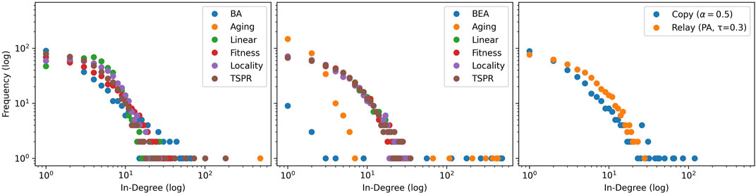
FIGURE 1. Mode-averaged in-degree distributions for simulated sum-normalized (left), softmax-normalized(centre), and other baseline models (right). 50 iterations of 500 node steps are run per model. Models in the same iteration number use identical, pre-drawn out-degree counts from
The models are further differentiated by subject signatures. Figure 2 shows that the baseline models do not reproduce intra-subject citations. Instead, citation densities are evenly spread across all subjects. As expected, this also applies to the softmax-normalized subject models (except Locality). The softmax function’s smoothing effect is particularly significant here because we use features — such as authority score and cosine similarities — that range within
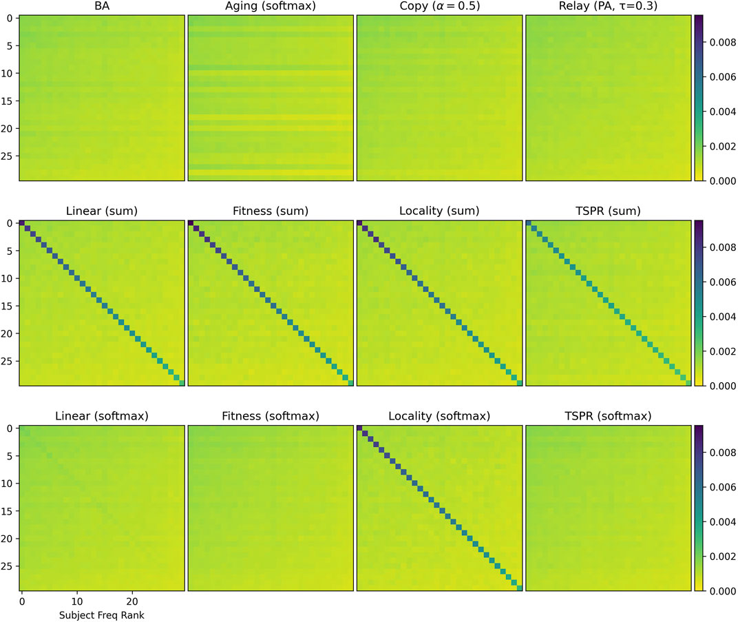
FIGURE 2.
The remaining subject models have largely similar subject signatures. To further distinguish them, we examine specific graph properties presented in Tables 1 and 2. While our subject models are similar to baselines in some respects like connectivity, they have clear structural differences, particularly in terms of subject communities.
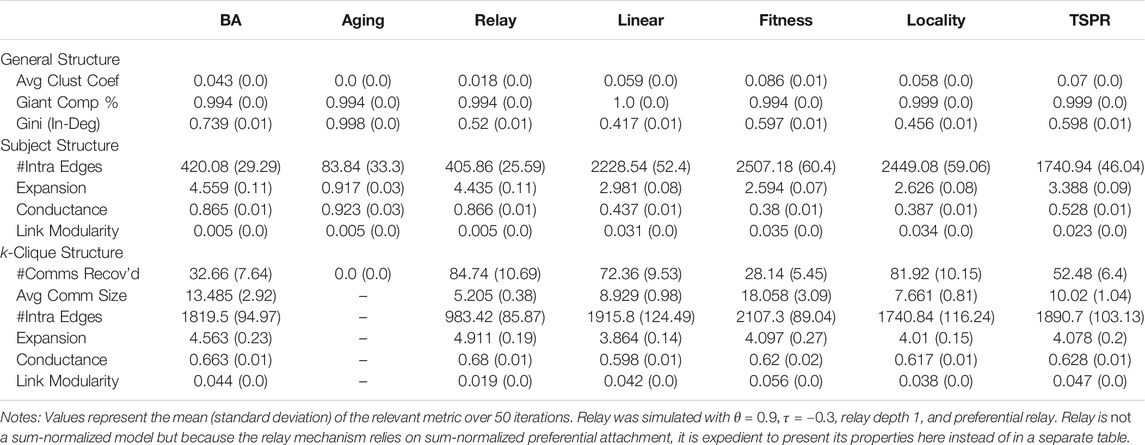
TABLE 1. Simulated properties for sum-normalized and relay models.
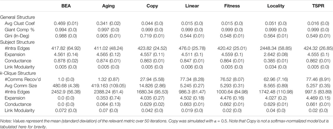
TABLE 2. Simulated properties for softmax-normalized and copying models.
General Properties: Clustering coefficients were generally low (save in the BEA and Aging (softmax) models). All models produced giant components encompassing most (around 99.9%) of the graph. However, in-degree distributions in baselines are generally more imbalanced than in the subject models. Gini coefficients for the baselines ranged between 0.52 (relay) to 0.998 (Aging (sum)) whereas those for the subject models ranged between 0.417 (Linear (sum)) to 0.598 (TSPR (sum)).
Subject Structure: Relative to all others, sum-normalized subject models yielded more intra-subject edges, lower expansion and conductance scores for communities defined by the gold labels, as well as higher link modularities. These networks therefore exhibit stronger within-subject clustering (an attribute which, to recall, should in theory characterize CLCNs). Conversely, the softmaxed subject models differed only slightly from the baselines. To be sure, stronger conformity with subject labels is not necessarily better, since legal citations are influenced by more than subject relevance alone. Depending on the extent of subject clustering desired, therefore, TSPR approaches may offer a middle-ground.
k-Clique Structure: The k-clique metrics paint a less coherent picture. There is no clear correlation between how well the models retrace gold label subjects and the average number, size, and quality of the communities recovered by k-clique percolation. The average number (size) of communities uncovered amongst sum-normalized subject models varies from around 28 to 82 (7–18) whereas the softmaxed subject models tend to yield around 70 k-clique communities of 5–8 nodes. Insofar as our models approximate the legal citation process, these results suggest that k-clique percolation may be less useful for clustering (and classifying) case law by legal subjects. Communities recovered by the algorithm do not appear to reflect actual legal areas, suggesting that legal subject clustering does not follow the assumptions of k-clique percolation. Nonetheless, the observed k-clique communities may be the result of other clustering mechanics inherent in legal citation networks. To this extent, they offer an independent basis for assessing the structural similarity of different simulated models. For instance, it is clear from Table 2 that the BEA model, which always results in exactly 1 large k-clique community that encapsulates the whole network, is structurally distinct from the rest. The sum-normalized Fitness and TSPR models also stand out from the other sum-normalized subject models as they tend to produce fewer but larger k-clique communities (see Table 1).
In sum, preliminary simulations demonstrate that the specific approach used to incorporate subject relevance induces significantly different network structures. While using subject cosine similarities as fitness values in a sum-normalized model may be theoretically similar to setting subject constraints on citable localities, the resulting networks differ in key aspects such as in-degree distribution and k-clique structure. The normalization function used also makes a key difference. This in turn underscores the importance of carefully selecting the subject model. Here we do not declare any one model as correct or best. To the extent that an ideal model exists, its parameterization likely turns on the specific type of CLCN we are trying to simulate. The legal and institutional context underlying the network would be relevant. Citation practices in one court at a given time may fall closer to the Fitness model, whereas another court may cite more in line with the TSPR model.
That said, it is also clear that certain subject models, especially those using softmax normalization, are unlikely to successfully capture the nuances of legal citations for the reasons given above. For benchmarking purposes, therefore, we focus on approaches that appear more promising, being Linear (sum), Fitness (sum), Locality (softmax), and TSPR (sum). For brevity, we only present results for more promising baselines as well (being BA, Copying, and Relay).10
3.2 Empirical Benchmarks
Figures 3 and 4 compare in-degree distributions produced by the calibrated baseline and subject models against actual distributions from the USSC and SGCA benchmarks respectively. Both benchmark distributions are broadly reproduced by all models (including baselines), though BA and Fitness (sum) produce slightly gentler-sloping distributions in both cases. At the same time, Figures 5 and 6 show that only the subject models successfully reproduce empirical subject signatures. To see this, first notice that since subject distributions for both the USSC and SGCA are imbalanced, citation densities are naturally concentrated within the top left quarter (which indexes the most frequent subjects). Second, observe that main diagonals for both benchmarks are also denser than their off-diagonals, showing that subject overlap materially influences actual legal citations. Although the general top-left concentration is reproduced by all models (recall that simulated subjects are drawn from a Dirichlet parameterized by actual subject frequencies), only subject models exhibit the benchmarks’ distinctive signature.

FIGURE 3. Mode-averaged in-degree distributions for USSC-calibrated baselines (left) and subject models (right) relative to the actual. Mirroring the actual network, 50 iterations of 2000 node steps are run per model. Models in the same iteration use identical, pre-drawn out-degree counts from
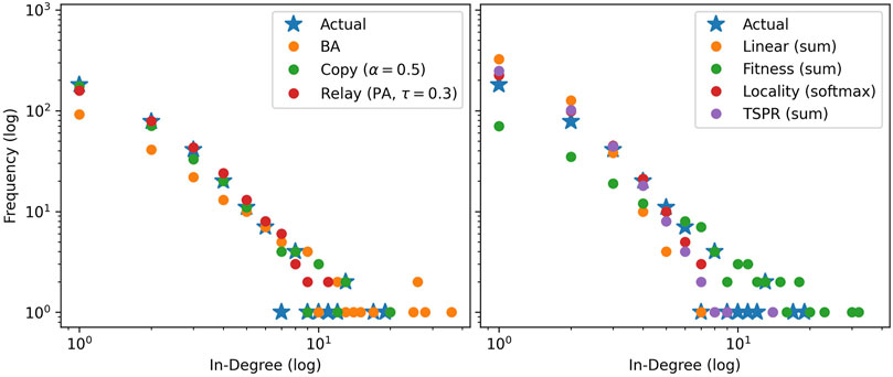
FIGURE 4. Mode-averaged in-degree distributions for SGCA-calibrated baselines (left) and subject models (right) relative to the actual. Mirroring the actual network, 50 iterations of 1000 node steps are run per model. Models in the same iteration use identical, pre-drawn out-degree counts from
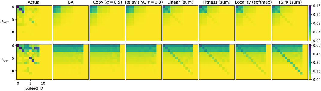
FIGURE 5.
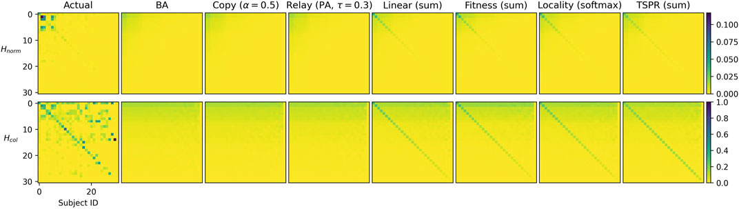
FIGURE 6.
These observations apply to both
Downward density gradients for the benchmarks’ signatures are noticeably less smooth than for the simulations. This is clearest for the SGCA benchmark, where (within the top 15 subjects) some less frequent subjects are more likely to be cited than the most frequent. This is suggestive of specific correlations between legal subjects. For example, subject 15 may be legally very relevant to and therefore often cited by subject 5 even though the former rarely occurs. Our models do not currently account for such subject covariance and future work could explore this further.
Figure 7 tabulates L1 distances between the benchmark and simulated networks and provides further confirmation that the subject models offer a closer approximation of CLCNs than baselines. Total, diagonal, off-diagonal, and column-wise distances are consistently smaller for the subject models than for the baselines. Note that results are similar if we include other (previously discussed) baselines, including alternative paramaterizations of Copying and Relay, and also if we use Kullbeck-Leibler divergence instead of L1 distance.11 Surprisingly, none of the subject models are clearly superior to the others. All clock in comparable numbers for every metric.
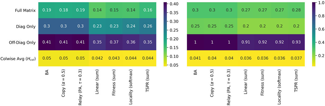
FIGURE 7. L1 distances for USSC-calibrated (left) and SGCA-calibrated models (right) relative to their respective benchmarks. Distances in the top three rows are computed from
Therefore, to determine which models produce better empirical fit, we look into detailed network properties for each benchmark as presented in Tables 3 and 4. Results here are consistent with the preliminary simulations. Clustering coefficients and giant component percentages for all models are broadly similar, but in-degree distributions vary across models.
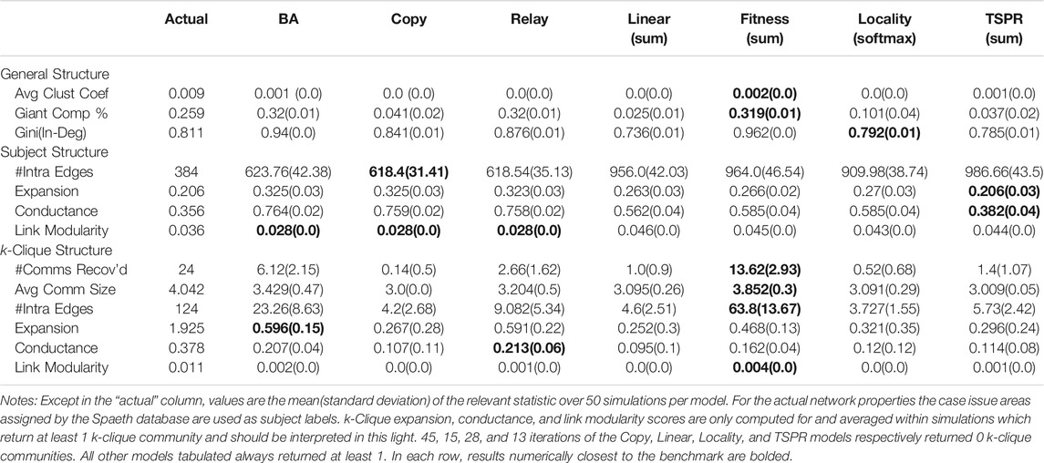
TABLE 3. Actual versus simulated properties for the USSC network.
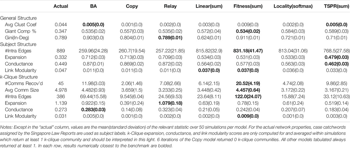
TABLE 4. Actual versus simulated properties for the SGCA network.
As expected, subject models yield networks with stronger subject communities than all baselines. The subject models fit the SGCA benchmark well, each producing around 800 intra-subject edges compared to the benchmark’s 889. They also yield expansion, conductance, and link modularity scores indicating better subject community quality. However, the community quality metrics for the benchmark’s network are even better, suggesting that our models can place even more weight on subject overlap.
Fit for the USSC benchmark is less clear. The USSC network has relatively few intra-subject edges. Resultantly, the baselines fall closer to the benchmark on this metric. However, community quality for the subject models are significantly closer to the actual. Re-creating the USSC network may therefore require model paramaterizations which create smaller but even more distinctive communities.
In terms of k-clique structure, the model closest to both benchmarks is Fitness (sum). The model produces on average 13.62 communities of 3.85 nodes (compared to 24 and 4.042) and 20.52 communities of size 4.452 (compared to 45 and 4.978) for the actual SGCA network). All other models yield significantly fewer k-clique communities. Indeed, 15 iterations of Linear (sum), 28 iterations of Locality (softmax), and 13 iterations of TSPR produced 0 k-clique communities. Conversely, Fitness (sum) always returns at least one k-clique community (including when calibrated with the SGCA network).
4 Discussion
The mechanics of case law citations involve complex interactions between the legal authority of a case, its relevance to the citer’s subjects, as well as the case’s age. We may represent the case law citation function in abstract as a probability distribution
In this light, this paper studied by simulation the expected properties of networks generated by the four approaches above and compared them against established network models. We then compared more promising models against two actual CLCNs from the USSC and SGCA respectively. Our findings underscore the importance of a legally-informed model of link generation process. The properties of all proposed subject models were substantially different from those of the baseline models, (provided that sum-normalization was used), and closer to empirical benchmarks in terms of both graph properties and subject signature.
Amongst the range of approaches studied, we found softmax normalization generally unsuited for the task because it smoothens away distinguishing differences in case attributes. We also see that model properties vary substantially when alternative means of modelling subject relevance were tested. All subject models performed comparably in terms of subject signature distance from both benchmarks. However, while three of the four subject models studied yielded average in-degree distributions very close to both benchmarks, the Fitness (sum) model yielded a noticeably gentler degree-rank slope. Nonetheless, Fitness (sum) best fits the k-clique structure of both benchmarks.
The emergent picture is that all subject models provide plausible (and superior to baseline) approaches for modelling CLCNs. For our two benchmarks, however, Fitness (sum) slightly edges out the other approaches as the most promising method for modelling CLCNs. To recall, this model takes the cosine similarity between the subject belonging vectors of two cases as a fitness coefficient that modifies the weight computed from each case’s authority and age. Notice that this model is similar to the General Temporal model in many respects, and may be seen as an extension of that model tailored to the legal citation context. An important caveat here is that although Fitness (sum) is relatively better when compared to alternative models, it is not in absolute terms a perfect approximation of either benchmark. Key differences remain between the actual and fitness-simulated networks. Further, alternative models may be better suited for CLCNs from other courts.
Our findings hint at possible universality in terms of the way courts think about subject relevance when deciding which cases to cite, though we hasten to add that the two benchmarks ran do not offer sufficient evidence. Universal or otherwise, the alternative models proposed may be useful for examining how courts and possibly individual judges differ when selecting cases to cite. If court/judge A’s citation network is better approximated by model X while court/judge B’s network is better approximated by model Y. Our models are also helpful for generating better simulated data that may be used to research other questions in legal network science. For instance, researchers could benchmark centrality algorithms against networks simulated with these models to study how far these algorithms recover legally-significant nodes. This, to recall Section 1, is a rich area of legal networks research. Since the data is simulated, it becomes possible to specifically dictate which nodes are legally-significant.
5 Limitations and Future Work
This paper is the first to study how the unique mechanics of case law citations may be simulated and studied using network models. As a first step, it necessarily leaves a number of important questions unexplored.
First, although we have identified promising approaches for modelling CLCNs, alternative models for legal authority, subject relevance, and time decay remain to be studied. We have focused on comparing different methods for modelling subject relevance because this is the least explored question. Nonetheless, the effect of varying authority and time-decay models are worth studying further. Varying time-decay models in particular may yield insights on how quickly the value of precedent depreciates (a question often raised by legal scholars [8, 39]), as well as how much deference different courts accord to antiquated precedent.
Second, future work can explore a larger space of model parameterizations. An immediate extension would be using time-variant network growth rates. That is, both λ and μ may vary across time. Further, the feature weights α, β, and γ may be adjusted to generate and also reflect different judicial attitudes towards assessing authority and relevance. It may be possible to learn these weights from empirical data, whether using exponential random graph models or machine learning techniques. This would provide a means of quantitatively measuring which factors most influence legal citation decisions, providing a common metric for comparing how these differ (or remain the same) across judges, time, and space.
Third, this study was limited by data availability. Despite growing literature in case law citations analysis, few publicly available edgelists can be linked to case-level (subject) metadata. For now, we have benchmarked our models against two empirical networks produced by apex Common Law courts. Future work can consider how closely these models approximate the citation mechanics of courts in other jurisdictions, particularly those of Civil Law jurisdictions where the doctrine of precedent theoretically holds less sway.
Fourth, while we have focused primarily on network structure, the microscopic properties of our proposed networks remain largely unexplored. Future work could use node-level metrics such as centrality and accessibility to study what kinds of cases and subjects are most likely to become entrenched in the core of such networks (e.g. [64]). Additionally, the task of replicating and studying CLCNs would also benefit from also exploiting the textual content of case judgments, as was done in [35]. Methods that exploit both network structure and node attributes for community detection (e.g. [65]) could be explored. This would connect our work to the growing literature on legal language processing (e.g. [66, 67]).
Data Availability Statement
The original contributions presented in the study are included in the article/Supplementary Material, further inquiries can be directed to the corresponding author.
Author Contributions
JS was in charge of all coding, data analysis, and writing.
Conflict of Interest
The author declares that the research was conducted in the absence of any commercial or financial relationships that could be construed as a potential conflict of interest.
Acknowledgments
We thank Daniel Katz, Michael Bommarito, Ryan Whalen, and Kenny Chng for insightful discussions on the topic, participants of the Physics of Law conference for valuable input, the editors of the special collection on the Physics of Law for inspiring this research, and three reviewers for constructive input. We thank also our loved ones for supporting our research unconditionally.
Supplementary Material
The Supplementary Material for this article can be found online at: https://www.frontiersin.org/articles/10.3389/fphy.2021.665563/full#supplementary-material
Footnotes
1All models and simulation methods are implemented in Python and will subsequently be made available in a GitHub repository.
2Though judgments often cite to other forms of law such as statutes. We leave these such hybrid networks aside for now.
3Judgments published close in time could cite one another. This occurs, albeit rarely, in the Singapore dataset below.
4Notice that this effectively models link probabilities with a multi-class logistic model.
5Other parameterizations for the copying (
6This includes the root node plus 500 node-time steps.
7Mean and median are not suitable here since they yield decimal values that would render frequency counts problematic. Where more than one mode exists we take the smallest value.
8To illustrate, if a node with subjects 1 and 2 cites a node with subjects 3 and 4, entries(3,1), (4,1), (3,2) and (4,2) are all incremented.
9We also experimented with Kullbeck-Leibler divergence and obtained similar results, though that measure often returns infinity.
10Results for the other baselines and varying paramaterizations of Copying and Relay(on file) do not affect our conclusions.
11Though Kullbeck-Leibler returns infinity on some graphs.
References
1. Clough JR, Gollings J, Loach TV, Evans TS. Transitive Reduction of Citation Networks. J Complex Networks (2015) 3:189–203. doi:10.1093/comnet/cnu039
2. Fowler JH, Johnson TR, Spriggs JF, Jeon S, Wahlbeck PJ. Network Analysis and the Law: Measuring the Legal Importance of Precedents at the U.S. Supreme Court. Polit Anal (2007) 15:324–46. doi:10.1093/pan/mpm011
3. Fowler JH, Jeon S. The Authority of Supreme Court Precedent. Soc. Networks (2008) 30:16–30. doi:10.1016/j.socnet.2007.05.001
4. Leibon G, Livermore M, Harder R, Riddell A, Rockmore D. Bending the Law: Geometric Tools for Quantifying Influence in the Multinetwork of Legal Opinions. Artif Intell L (2018) 26:145–67. doi:10.1007/s10506-018-9224-2
5. Derlén M, Lindholm J. Characteristics of Precedent: The Case Law of the European Court of Justice in Three Dimensions. Ger Law J (2015) 16:1073–98. doi:10.1017/S2071832200021040
6. Lupu Y, Voeten E. Precedent in International Courts: A Network Analysis of Case Citations by the European Court of Human Rights. Br J. Polit. Sci. (2012) 42:413–39. doi:10.1017/S0007123411000433
7. Soh J. A Network Analysis of the Singapore Court of Appeal's Citations to Precedent. SSRN J (2019) 31:246–84. doi:10.2139/ssrn.3346422
8. Whalen R, Uzzi B, Mukherjee S. Common Law Evolution and Judicial Impact in the Age of Information. Elon L Rev (2017) 9:115–70.
9. Bommarito MJ, Katz DM. Properties of the United States Code Citation Network (2010). Available from: https://https://arxiv.org/abs/0911.1751 (Accessed 09 July, 2021).
10. Katz DM, Coupette C, Beckedorf J, Hartung D. Complex Societies and the Growth of the Law. Sci Rep (2020) 10:18737. ArXiv: 2005.07646. doi:10.1038/s41598-020-73623-x |
11. Coupette C, Beckedorf J, Hartung D, Bommarito M, Katz DM. Measuring Law over Time: A Network Analytical Framework with an Application to Statutes and Regulations in the United States and Germany. Front Physics (2021) 9:269. doi:10.3389/fphy.2021.658463
12. Watts D, Strogatz S. Collective Dynamics of 'Small-World' Networks. Nature (1998) 393:3. doi:10.1038/30918 |
13. Girvan M, Newman MEJ. Community Structure in Social and Biological Networks. Proc Natl Acad Sci (2002) 99:7821–6. Institution: National Academy of Sciences Publisher: National Academy of Sciences Section: Physical Sciences. doi:10.1073/pnas.122653799 |
14. Porter MA, Onnela JP, Mucha PJ. Communities in Networks. Notices Am Math Soc (2009) 56:1082–166.
15. Holland PW, Laskey KB, Leinhardt S. Stochastic Blockmodels: First Steps. Soc Networks (1983) 5:109–37. doi:10.1016/0378-8733(83)90021-7
16. Karrer B, Newman MEJ. Stochastic Blockmodels and Community Structure in Networks. Phys Rev E (2011) 83:016107. doi:10.1103/PhysRevE.83.016107 |
17. Newman MEJ. Fast Algorithm for Detecting Community Structure in Networks. Phys Rev E (2004) 69:066133. doi:10.1103/PhysRevE.69.066133 |
18. Newman MEJ, Girvan M. Finding and Evaluating Community Structure in Networks. Phys Rev E (2004) 69:026113. doi:10.1103/PhysRevE.69.026113 |
19. Clauset A, Newman MEJ, Moore C. Finding Community Structure in Very Large Networks. Phys Rev E (2004) 70:066111. doi:10.1103/PhysRevE.70.066111 |
20. Derényi I, Palla G, Vicsek T. Clique Percolation in Random Networks. Phys Rev Lett (2005) 94:160202. doi:10.1103/PhysRevLett.94.160202 |
21. Newman MEJ. Finding Community Structure in Networks Using the Eigenvectors of Matrices. Phys Rev E (2006) 74:036104. doi:10.1103/PhysRevE.74.036104 |
22. Nicosia V, Mangioni G, Carchiolo V, Malgeri M. Extending the Definition of Modularity to Directed Graphs with Overlapping Communities. J Stat Mech (2009) 2009:P03024. doi:10.1088/1742-5468/2009/03/P03024
23. Mucha PJ, Richardson T, Macon K, Porter MA, Onnela J-P. Community Structure in Time-dependent, Multiscale, and Multiplex Networks. Science (2010) 328:876–8. doi:10.1126/science.1184819 |
24. Chen M, Szymanski BK. Fuzzy Overlapping Community Quality Metrics. Soc Netw Anal Min (2015) 5:40. doi:10.1007/s13278-015-0279-8
25. Bommarito MJ, Katz DM, Zelner JL, Fowler JH. Distance Measures for Dynamic Citation Networks. Physica A: Stat Mech its Appl (2010) 389:4201–8. doi:10.1016/j.physa.2010.06.003
26. Mirshahvalad A, Lindholm J, Derlén M, Rosvall M. Significant Communities in Large Sparse Networks. PLoS One (2012) 7:e33721. Public Library of Science. doi:10.1371/journal.pone.0033721 |
27. Sulea OM, Zampieri M, Malmasi S, Vela M, Dinu LP, van Genabith J. Exploring the Use of Text Classification in the Legal Domain (2017) Minneapolis, Minnesota, 2-7 June 2019 CoRR abs/1710.09306.
28. Soh J, Lim HK, Chai IE. Legal Area Classification: A Comparative Study of Text Classifiers on Singapore Supreme Court Judgments. In: Proceedings of the Natural Legal Language Processing Workshop 2019. Minneapolis, Minnesota: Association for Computational Linguistics (2019). 67–77. doi:10.18653/v1/W19-2208
29. de Solla Price DJ. Networks of Scientific Papers. Science (1965) 149:510–5. Institution: American Association for the Advancement of Science Section: Articles. doi:10.1126/science.149.3683.510 |
30. Broido AD, Clauset A. Scale-free Networks Are Rare. Nat Commun (2019) 10(1):1017. Institution: Nature Publishing Group. doi:10.1038/s41467-019-08746-5 |
31. Wang M, Yu G, Yu D. Effect of the Age of Papers on the Preferential Attachment in Citation Networks. Physica A: Stat Mech its Appl (2009) 388:4273–6. doi:10.1016/j.physa.2009.05.008
32. Menczer F. Evolution of Document Networks. Proc Natl Acad Sci (2004) 101:5261–5. doi:10.1073/pnas.0307554100 |
33. Singh M, Sarkar R, Goyal P, Mukherjee A, Chakrabarti S. Relay-Linking Models for Prominence and Obsolescence in Evolving Networks. In: Proceedings of the 23rd ACM SIGKDD International Conference on Knowledge Discovery and Data Mining, Halifax, Nova Scotia, 13-17 August 2017 (2017). 1077–86. ArXiv: 1609.08371. doi:10.1145/3097983.3098146
34. Kumar R, Raghavan P, Rajagopalan S, Sivakumar D, Tomkins A, Upfal E. Stochastic Models for the Web Graph. In: Proceedings 41st Annual Symposium on Foundations of Computer Science. 12-14 November 2000, Redondo Beach, CA: IEEE Comput. Soc (2000). 57–65. doi:10.1109/SFCS.2000.892065
35. Amancio DR, Oliveira ON, da Fontoura Costa L. Three-feature Model to Reproduce the Topology of Citation Networks and the Effects from Authors' Visibility on Their H-index. J Informetrics (2012) 6:427–34. doi:10.1016/j.joi.2012.02.005
36. Bianconi G, Barabási A-L. Competition and Multiscaling in Evolving Networks. Europhys Lett (2001) 54:436–42. doi:10.1209/epl/i2001-00260-6
37. Li X, Chen G. A Local-World Evolving Network Model. Physica A: Stat Mech its Appl (2003) 328:274–86. doi:10.1016/S0378-4371(03)00604-6
38. Haveliwala TH. Topic-sensitive Pagerank. In: Proceedings of the 11th International Conference on World Wide Web, 7-11 May 2002, New York, NY, USA: Association for Computing Machinery (2002). 517–526. doi:10.1145/511446.511513
39. Posner R. An Economic Analysis of the Use of Citations in the Law. Am L Econ Rev (2000) 2:381–406. doi:10.1093/aler/2.2.381
40. Carmichael I, Wudel J, Kim M, Jushchuk J. Examining the Evolution of Legal Precedent Through Citation Network Analysis. N. C. Law Rev. (2017) 96:44. https://scholarship.law.unc.edu/nclr/vol96/iss1/6/
41. Barabasi AL, Albert R. Emergence of Scaling in Random Networks. Science (1999) 286:4. doi:10.1126/science.286.5439.509 |
42. Medo M, Cimini G, Gualdi S. Temporal Effects in the Growth of Networks. Phys Rev Lett (2011) 107:238701. doi:10.1103/PhysRevLett.107.238701 |
43. Ii MJB, Katz DM, Zelner JL. On the Stability of Community Detection Algorithms on Longitudinal Citation Data. Proced - Soc Behav Sci (2010) 4:26–37. doi:10.1016/j.sbspro.2010.07.480
44. Pham T, Sheridan P, Shimodaira H. PAFit: A Statistical Method for Measuring Preferential Attachment in Temporal Complex Networks. PLoS One (2015) 10:e0137796. doi:10.1371/journal.pone.0137796 |
45. Hajra KB, Sen P. Aging in Citation Networks. Physica A: Stat Mech its Appl (2005) 346:44–8. doi:10.1016/j.physa.2004.08.048
46. Cormode G, Shkapenyuk V, Srivastava D, Xu B. Forward Decay: A Practical Time Decay Model for Streaming Systems. In: 2009 IEEE 25th International Conference on Data Engineering, 29 March-2 April 2009, Shanghai, China: IEEE (2009). 138–49. doi:10.1109/ICDE.2009.65
47. Caldarelli G, Capocci A, De Los Rios P, Muñoz MA. Scale-Free Networks from Varying Vertex Intrinsic Fitness. Phys Rev Lett (2002) 89:258702. doi:10.1103/PhysRevLett.89.258702 |
48. Sun J, Staab S, Karimi F. Decay of Relevance in Exponentially Growing Networks. In: Proceedings of the 10th ACM Conference on Web Science, 30 June-3 July 2019, Boston, MA (2018) 343–51. doi:10.1145/3201064.3201084
49. Mikolov T, Sutskever I, Chen K, Corrado GS, Dean J. Distributed Representations of Words and Phrases and Their Compositionality. In: CJC Burges, L Bottou, M Welling, Z Ghahramani, and KQ Weinberger, editors. Advances in Neural Information Processing Systems 26. Curran Associates, Inc.) (2013). 3111–9.
50. Chen DL, Ash E, Livermore MA. Case Vectors: Spatial Representations of the Law Using Document Embeddings. In: DN Rockmore, editor. Law as Data: Computation, Text, & the Future of Legal Analysis. Santa Fe: SFI Press (2019). HOLLIS number: 99153793511303941
51. Kleinberg JM. Authoritative Sources in a Hyperlinked Environment. J ACM (1999) 46:604–32. doi:10.1145/324133.324140
52. Cross FB, Spriggs JFI. The Most Important(And Best) Supreme Court Opinions and Justices. Emory Law J. (2010) 60:407–502. https://scholarlycommons.law.emory.edu/elj/vol60/iss2/5/
53. Blei DM, Ng AY, Jordan MI. Latent Dirichlet Allocation. J Machine Learn Res (2003) 3:993–1022. doi:10.5555/944919.944937
54. Bhattacharya P, Ghosh K, Pal A, Ghosh S. Methods for Computing Legal Document Similarity: A Comparative Study . Madrid, Spain: 5th Workshop on Legal Data Analysis (2019).
55. Brin S, Page L. The PageRank Citation Ranking: Bringing Order to the Web (1998). Available from: http://ilpubs.stanford.edu:8090/422/1/1999-66.pdf (Accessed 09 July, 2021).
56. Hagberg AA, Schult DA, Swart PJ. Exploring Network Structure, Dynamics, and Function Using Networkx. In: G Varoquaux, T Vaught, and J Millman, editors. Proceedings of the 7th Python in Science Conference. Pasadena, CA: (2008). 11–5.
57. Radicchi F, Castellano C, Cecconi F, Loreto V, Parisi D. Defining and Identifying Communities in Networks. Proc Natl Acad Sci 101. Institution: National Academy of Sciences Section: Physical Sciences (2004). 2658–63. doi:10.1073/pnas.0400054101 |
58. Palla G, Farkas IJ, Pollner P, Derényi I, Vicsek T. Directed Network Modules. New J Phys (2007) 9:186. doi:10.1088/1367-2630/9/6/186
59. Rossetti G, Milli L, Cazabet R. CDLIB: a python Library to Extract, Compare and Evaluate Communities from Complex Networks. Appl Netw Sci (2019) 4(1):1–26. Institution: Springer. doi:10.1007/s41109-019-0165-9
60. Spaeth HJ, Epstein L, Martin AD, Segal JA, Ruger TJ, Benesh SC. The Supreme Court Database. Version 2017 Release 1. St Louis, Missouri: Publication Title: The Supreme Court Database (2017).
61. Donnat C, Holmes S. Tracking Network Dynamics: A Survey Using Graph Distances. Ann Appl Stat (2018) 12:971–1012. doi:10.1214/18-AOAS1176
62. Hammond DK, Gur Y, Johnson CR. Graph Diffusion Distance: A Difference Measure for Weighted Graphs Based on the Graph Laplacian Exponential Kernel. in: 2013 IEEE Global Conference on Signal and Information Processing, 3-5 December 2013, Austin, TX (2013). 419–22. doi:10.1109/GlobalSIP.2013.6736904
63. Xu Y, Salapaka SM, Beck CL. A Distance Metric between Directed Weighted Graphs. In: 52nd IEEE Conference on Decision and Control, 10-13 December 2013, Firenze: IEEE (2013). p. 6359–64. doi:10.1109/CDC.2013.6760895
64. Amancio DR, Nunes MGV, Oliveira ON, Costa Ld. F. Extractive Summarization Using Complex Networks and Syntactic Dependency. Physica A: Stat Mech its Appl (2012) 391:1855–64. doi:10.1016/j.physa.2011.10.015
65. Yang J, McAuley J, Leskovec J. Community Detection in Networks with Node Attributes. In: 2013 IEEE 13th International Conference on Data Mining, 7-10 December 2013, Dallas, TX (2013). 1151–6. doi:10.1109/ICDM.2013.167
66. Aletras N, Tsarapatsanis D, Preoţiuc-Pietro D, Lampos V. Predicting Judicial Decisions of the European Court of Human Rights: A Natural Language Processing Perspective. PeerJ Comput Sci (2016) 2:e93. doi:10.7717/peerj-cs.93
Keywords: case law citation networks, legal network science, physics of law, network modelling, community detection
Citation: Soh Tsin Howe J (2021) Simulating Subject Communities in Case Law Citation Networks. Front. Phys. 9:665563. doi: 10.3389/fphy.2021.665563
Received: 08 February 2021; Accepted: 02 July 2021;
Published: 16 July 2021.
Edited by:
J.B. Ruhl, Vanderbilt University, United StatesReviewed by:
Animesh Mukherjee, Indian Institute of Technology Kharagpur, IndiaDiego R Amancio, University of São Paulo, Brazil
Arthur Dyevre, KU Leuven, Belgium
Copyright © 2021 Soh Tsin Howe. This is an open-access article distributed under the terms of the Creative Commons Attribution License (CC BY). The use, distribution or reproduction in other forums is permitted, provided the original author(s) and the copyright owner(s) are credited and that the original publication in this journal is cited, in accordance with accepted academic practice. No use, distribution or reproduction is permitted which does not comply with these terms.
*Correspondence: Jerrold Soh Tsin Howe, jerroldsoh@smu.edu.sg