End point gradient estimates for quasilinear parabolic equations with variable exponent growth on nonsmooth domains

Abstract

In this paper, we study quasilinear parabolic equations with the nonlinearity structure modeled after the p(x, t)-Laplacian on nonsmooth domains. The main goal is to obtain end point Calderón-Zygmund type estimates in the variable exponent setting. In a recent work [1], the estimates obtained were strictly above the natural exponent p(x, t) and hence there was a gap between the natural energy estimates and the estimates above p(x, t) (see (1.3) and (1.2)). Here, we bridge this gap to obtain the end point case of the estimates obtained in [1]. To this end, we make use of the parabolic Lipschitz truncation developed in [2] and obtain significantly improved a priori estimates below the natural exponent with stability of the constants. An important feature of the techniques used here is that we make use of the unified intrinsic scaling introduced in [3], which enables us to handle both the singular and degenerate cases simultaneously.

Appendices

The method of Lipschitz truncation–first difference estimate

In this appendix, following the techniques developed in [3] which were originally pioneered in [2], we will develop a modified version of Lipschitz truncation suited to our needs. Recall that u is a weak solution of (1.1) and w is a weak solution of (6.17). For this section, we only need to assume the following restrictions on the size of the region $K_{4\rho }^{\alpha }(\mathfrak {z})$: In particular, we will take $\tilde{\rho }_3$ small such that (R6) and (R4) are applicable.

To simplify the notation, we will define

$$\begin{aligned} s:{=} \alpha ^{-1+d} (4\rho )^2. \end{aligned}$$

(A.1)

Let us now collect some well known results that will be needed in the course of the proof. The first lemma is a time localised version of the parabolic Poincaré inequality (see [34, Lemma 4.2] for the proof):

Lemma A.1

Let $f \in L^{\vartheta } (-T,T; W^{1,\vartheta }(\Omega ))$ with $\vartheta \in (1,\infty )$ and suppose that $\mathcal {B}_{r} \Subset \Omega$ be compactly contained ball of radius $r>0$. Let $I \subset (-T,T)$ be a time interval and $\rho (x,t) \in L^1(\mathcal {B}_r \times I)$ be any positive function such that

$$\begin{aligned} \Vert \rho \Vert _{L^{\infty }(\mathcal {B}_r\times I)} \lesssim _{(n)} \frac{|\mathcal {B}_r\times I|}{\Vert \rho \Vert _{L^1(\mathcal {B}_r\times I)}} \end{aligned}$$

and $\mu (x) \in C_c^{\infty }(\mathcal {B}_r)$ be such that $\int _{\mathcal {B}_r} \mu (x) \ dx = 1$ with $|\mu | \le \frac{C_{(n)}}{r^n}$ and $|\nabla \mu | \le \frac{C_{(n)}}{r^{n+1}}$, then there holds:

where , and $J \Subset (-\infty ,\infty )$ is some fixed time-interval.

Lemma A.2

For any $h \in (0,2s)$ and let $\phi (x) \in C_c^{\infty }({\Omega _{4\rho }^{\alpha }(\mathfrak {x})})$ and $\varphi (t) \in C^{\infty }(\mathfrak {t}-s,\infty )$ with $\varphi (\mathfrak {t}-s) = 0$ be a non-negative function and $[u]_h,[w]_h$ be the Steklov average as defined in (3.2). Then the following estimate holds for any time interval $(t_1,t_2) \subset [\mathfrak {t}-s,\mathfrak {t}+s]$:

1.1 Construction of test function

Let us denote the following functions:

$$\begin{aligned} v(z) :{=} u(z) - w(z) \qquad \text {and} \qquad v_h(z) :{=} [u-w]_h(z), \end{aligned}$$

where $[u-w]_h(z)$ denotes the usual Steklov average. It is easy to see that $v_h\xrightarrow {h \searrow 0} v$. We also note that $v(z) = 0$ for $z \in \partial _p K_{4\rho }^{\alpha }(\mathfrak {z})$. For some fixed $\mathfrak {q}$ such that $1<\mathfrak {q}< \frac{p^-}{p^+-1}$, with $\mathcal {M}$ as given in (5.2), let us now define

(A.2)

For a fixed $\lambda \ge 1$, let us define the good set by

(A.3)

For the rest of this section, we will always assume that the following bound holds:

Lemma A.3

With $\rho \le \tilde{\rho }_3$, there holds

Proof

Since $p(\cdot )\in p^{\pm }_{\log }$, we have from Remark 2.4,

Since $\rho \le 1$, we only need to bound $\rho ^{-(p^+_{K_{4\rho }^{\alpha }(\mathfrak {z})}-p^-_{K_{4\rho }^{\alpha }(\mathfrak {z})})}$, which we do as follows:

This completes the proof of the lemma.

Following the ideas from [3, Lemma 5.10], we can obtain a Vitali-type covering lemma.

Lemma A.4

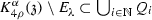
Let $\lambda \ge 1$ be such that (A.3) is given, then for every , consider the parabolic cylinders of the form

$$\begin{aligned} Q_{\rho _z}^{\lambda }(z) :{=} B_{\lambda ^{-\frac{1}{p(z)}+\frac{d}{2}}\rho _z}(x) \times (t - \lambda ^{-1+d}\rho _z^2,t + \lambda ^{-1+d}\rho _z^2) \end{aligned}$$

where Let $\mathfrak {k} \in (0,1]$ be a given constant and consider the open covering of given by

Then there exists a universal constant $\mathfrak {X}= \mathfrak {X}(p^{\pm }_{\log },n)\ge 9$ and a countable disjoint subcollection $\mathcal {G}:{=} \{Q_{\rho _i}^{\lambda }(z_i)\}_{i \in \mathbb {N}}\subset \mathcal {F}$ such that there holds

$$\begin{aligned} \bigcup _{\mathcal {F}}Q_{\mathfrak {k}\rho _z}^{\lambda }(z) \subset \bigcup _{\mathcal {G}} Q_{\mathfrak {X}\rho _{z_i}}^{\lambda } (z_i). \end{aligned}$$

We now have the following Whitney type covering whose proof is very similar to [3, Lemma 5.11].

Lemma A.5

There exists a universal constant $\delta \in (0,1/4)$ such that for $\mathcal {F}$, a given covering of given by the cylinders: where $\mathfrak {X}$ is the constant from Lemma A.4, there exists a countable subcollection $\mathcal {G}= \left\{ Q_{\delta \rho _{z_i}}^{\lambda }(z_i)\right\} _{i \in \mathbb {N}} = \{ Q_{r_i}^{\lambda }(z_i)\}_{i \in \mathbb {N}}$ subordinate to the covering $\mathcal {F}$ such that the following holds:

(W1):

.

(W2):

Each point belongs to utmost $C_{(n,p^{\pm }_{\log })}$ cylinders of the form $2Q_i$.

(W3):

There exists a constant $C=C_{(n,p^{\pm }_{\log })}$ such that for any two cylinders $Q_i$ and $Q_j$ with $2Q_i \cap 2Q_j \ne \emptyset$, there holds

$$\begin{aligned} |B_i| \le C |B_j| \le C |B_i| \qquad \text {and} \qquad |I_i| \le C |I_j| \le C |I_i|. \end{aligned}$$

In particular, there holds $|Q_i| \approx _{(p^{\pm }_{\log },n)} |Q_j|$.

(W4):

There exists a constant $\hat{c} = \hat{c}_{(n,p^{\pm }_{\log })}\ge 9$ such that for all $i \in \mathbb {N}$, there holds:

(W5):

For the constant $\hat{c}$ from above, there holds $2Q_i \cap 2Q_j \ne \emptyset$ implies $2Q_i \subset \hat{c}Q_j$.

Once we have obtained the Whitney type covering lemma, we can now obtain the following standard partition of unity lemma:

Lemma A.6

Subordinate to the covering $\mathcal {G}$ obtained in Lemma A.5 , we obtain a partition of unity that satisfies the following properties:

• $\sum _{i=1}^{\infty } \psi _i(z) = 1$ for all .

• $\psi _i \in C_c^{\infty }(2Q_i)$.

• $\Vert \psi _i\Vert _{\infty } + \lambda ^{-\frac{1}{p(z_i)}+\frac{d}{2}} r_i \Vert \nabla \psi _i\Vert _{\infty } + \lambda ^{-1+d} r_i^2 \Vert \partial _t \psi _i\Vert _{\infty } \le C_{(p^{\pm }_{\log },n)}$ where we have used the notation $r_i :{=} \delta \rho _{z_i}$ which is the parabolic radius of $Q_i$ with respect to the metric $d_{z_i}^{\lambda }$ (see Lemma A.5 for the notation).

• $\psi _i \ge C_{(p^{\pm }_{\log },n)}$ on $Q_i$.

Before we end this subsection, let us recall the following useful bound that will be used throughout this section. For a proof, see the proof of [3, Lemma 5.10, (5.23)].

$$\begin{aligned} \lambda ^{p^+_{2Q_i} - p^-_{2Q_i}} \le C_{(p^{\pm }_{\log },n)}. \end{aligned}$$

(A.4)

1.2 Construction of Lipschitz truncation function

Let us first clarify some of the notation that will subsequently be used in the rest of this section: for $\hat{c}$ from (W4), we denote

$$\begin{aligned} \hat{Q}_i :{=} \hat{c}Q_i = Q_{\hat{r}_i}^{\lambda }(z_i), \qquad \text {where} \qquad \hat{r}_i :{=} \hat{c} r_i. \end{aligned}$$

We shall also use the notation

$$\begin{aligned} \mathcal {I}(i) :{=} \{ j \in \mathbb {N}: {{\,\mathrm{spt}\,}}(\psi _i) \cap {{\,\mathrm{spt}\,}}(\psi _j) \ne \emptyset \} \qquad \text {and} \qquad \mathcal {I}_z :{=} \{ j \in \mathbb {N}: z \in {{\,\mathrm{spt}\,}}(\psi _j) \}. \end{aligned}$$

We are now ready to construct the Lipschitz truncation function:

(A.5)

where we have defined

(A.6)

From construction in (A.5) and (A.6), we see that

We see that has the right support for the test function and hence the rest of this section will be devoted to proving the Lipschitz regularity of on $K_{4\rho }^{\alpha }(\mathfrak {x})$ as well as some useful estimates.

1.3 Some estimates on the test function

In this subsection, we will collect some useful estimates on the test function. The proofs of these estimates follow similarly to those in [3] and hence we will only provide an outline of the proofs.

Lemma A.7

Let , then from (W1), we have that $\mathfrak {z}\in 2Q_i$ for some $i \in \mathcal {I}_{\mathfrak {z}}$. For any $1 \le \theta \le \frac{p^-}{\mathfrak {q}}$, there holds

(A.7)

(A.8)

Proof

Proof of (A.7): We prove this estimate as follows:

Proof of (A.8): From (A.3), we see that

Corollary A.8

For any , we have $z \in 2Q_i$ for some $i \in \mathcal {I}_{z}$, then there holds

$$\begin{aligned} |v_h(z)| \lesssim _{(n,p^{\pm }_{\log },\Lambda _0,\Lambda _1)}(\alpha ^{-\frac{1}{p(\mathfrak {z})}+\frac{d}{2}}\rho ) \lambda ^{\frac{1}{p(z_i)}}, \end{aligned}$$

where $z_i$ is the centre of $Q_i$.

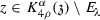
Lemma A.9

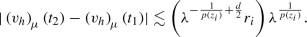
Let $2Q_i$ be a parabolic Whitney type cylinder, then for any $1 \le \theta \le \frac{p^-}{\mathfrak {q}}$, there holds

Proof

Let us consider the following two cases:

• Case $\alpha ^{-\frac{1}{p(\mathfrak {z})}+\frac{d}{2}}\rho \le \lambda ^{-\frac{1}{p(z_i)}+\frac{d}{2}}r_i$: In this case, we can use triangle inequality along with (A.7) to get

  

  (A.9)

• Case $\alpha ^{-\frac{1}{p(\mathfrak {z})}+\frac{d}{2}}\rho \ge \lambda ^{-\frac{1}{p(z_i)}+\frac{d}{2}}r_i$: Applying Lemma A.2 with $\mu \in C_c^{\infty }(2B_i)$ such that $|\mu (x)| \lesssim \frac{1}{\left(\lambda ^{-\frac{1}{p(z_i)}+\frac{d}{2}} r_i\right)^n}$ and $|\nabla \mu (x)| \lesssim \frac{1}{\left(\lambda ^{-\frac{1}{p(z_i)}+\frac{d}{2}} r_i\right)^{n+1}}$, we get

  

  (A.10)

  The first term on the right of (A.10) can be estimated using (A.8) to get

  

  (A.11)

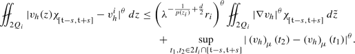
  To estimate the second term on the right of (A.10), we make use of Lemma A.2 with $\phi (x) = \mu (x)$ and $\varphi (t) \equiv 1$, we get

  

  (A.12)

  Now making use of (A.4) along with the fact that $\lambda \ge 1$ and $p^-_{2Q_i} \le p(z_i)$, we get

  $$\begin{aligned} \lambda ^{-1+ \frac{1}{p(z_i)} + \frac{p^+_{2Q_i}}{p^-_{2Q_i}} - \frac{1}{p^-_{2Q_i}}} = \lambda ^{\frac{p^+_{2Q_i}-p^-_{2Q_i}}{p^-_{2Q_i}}} \lambda ^{\frac{p^-_{2Q_i}-p(z_i)}{p(z_i)p^-_{2Q_i}}} \le \lambda ^{\frac{p^+_{2Q_i}-p^-_{2Q_i}}{p^-_{2Q_i}}} \overset{(A.4)}{\lesssim } C_{(p^{\pm }_{\log },n)}. \end{aligned}$$

  (A.13)

  Substituting (A.13) into (A.12), we get

  

  (A.14)

  Thus combining (A.11) and (A.14) into (A.10), we get

  

  which proves the lemma.

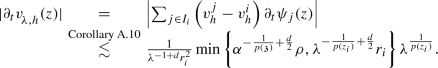
Corollary A.10

For any $i \in \mathbb {N}$ and any $j \in \mathcal {I}_i$, there holds

$$\begin{aligned} |v_h^i - v_h^j| \lesssim _{(p^{\pm }_{\log },\Lambda _0,\Lambda _1,n)} \min \left\{ \alpha ^{-\frac{1}{p(\mathfrak {z})}+\frac{d}{2}}\rho , \lambda ^{-\frac{1}{p(z_i)}+\frac{d}{2}}r_i\right\} \lambda ^{\frac{1}{p(z_i)}}. \end{aligned}$$

1.4 Bounds on and

Lemma A.11

Let $Q_i$ be a parabolic Whitney type cylinder. Then for any $z \in 2Q_i$, we have the following bound:

(A.15)

Corollary A.12

Let , then $z \in 2Q_i$ for some $i \in \mathbb {N}$. Then there holds for any $\delta \in (0,1]$, the estimates

(A.16)

(A.17)

Lemma A.13

Let , then $z \in 2Q_i$ for some $i \in \mathbb {N}$. Then there holds for any $\delta \in (0,1]$, the estimates

(A.18)

1.5 Estimates on the time derivative of

Lemma A.14

Let $z \in {K_{4\rho }^{\alpha }(\mathfrak {z})}$, then $z \in 2Q_i$ for some $i \in \mathbb {N}$. We then have the following estimates for the time derivative of :

(A.19)

We also have the improved estimate

(A.20)

Proof

Let us prove each of the assertions as follows:

• Estimate (A.19): In this case, we proceed as follows

  

• Estimate (A.20): From the fact that $\sum _{j \in I_i} \psi _j(z) = 1$, we see that $\sum _{j \in I_i} \partial _t \psi _j(z) = 0$ which along with Lemma A.6 gives the following sequence of estimates

  

1.6 Some important estimates for the test function

Lemma A.15

Let $Q_i$ be a Whitney-type parabolic cylinder for some $i \in \mathbb {N}$. Then for any $\vartheta \in [1,2]$, there holds

Lemma A.16

Let $Q_i$ be a Whitney-type parabolic cylinder for some $i \in \mathbb {N}$, then there holds

Lemma A.17

Let $Q_i$ be a Whitney-type parabolic cylinder for some $i \in \mathbb {N}$, then there holds

Proof

From (W2), we see that , thus for a given $i \in \mathbb {N}$, let use define the following

Making use of (A.20), we get

Summing over all $i \in \mathbb {N}$, we get the desired inequality.

1.7 Lipschitz continuity estimates

We will now show that the function constructed in (A.5) is Lipschitz continuous on $B_{4\rho }^{\alpha }(\mathfrak {x}) \times (\mathfrak {t}-s,\mathfrak {t}+s)$ where s is as defined in (A.1). To do this, we shall use the integral characterization of Lipschitz continuous functions obtained in [35, Theorem 3.1] which says the following:

Lemma A.18

(Lipschitz characterization) Let $\tilde{z}\in B_{4\rho }^{\alpha }(\mathfrak {x}) \times (\mathfrak {t}-s,\mathfrak {t}+s)$ and $r >0$ be given. Define the parabolic cylinder $Q_r(\tilde{z}) :{=} B_r(\tilde{x}) \times (\tilde{t}- r^2, \tilde{t}+r^2)$, i.e., $Q_r(\tilde{z}) :{=} \{ z \in \mathbb {R}^{n+1}: d_p(z,\tilde{z}) \le r\}$ where $d_p$ is as defined in Definition 2.1. Furthermore suppose that the following expression is bounded independent of $\tilde{z}\in B_{4\rho }^{\alpha }(\mathfrak {x}) \times (\mathfrak {t}-s,\mathfrak {t}+s)$ and $r>0$

then .

Remark A.19

From (2.7) and the fact that $\alpha \ge 1$, for any $\tilde{z}_1,\tilde{z}_2 \in \mathbb {R}^{n+1}$ and any $\tilde{z}\in \mathbb {R}^{n+1}$, we get

$$\begin{aligned} \begin{array}{rcl} d_p(\tilde{z}_1,\tilde{z}_2) &{} \overset{\text {Definition} 2.1}{:{=}} &{} \max \left\rbrace |x_1-x_2|, \sqrt{|t_1-t_2|} \right\lbrace \\ &{} \le &{} \max \left\{ \alpha ^{\frac{1}{p(z)}-\frac{d}{2}}|x_1-x_2|, \sqrt{\alpha ^{1-d} |t_1-t_2|} \right\} \overset{\text {Definition} 2.2}{ =:} d_{\tilde{z}}(\tilde{z}_1,\tilde{z}_2)\\ &{} \le &{} \alpha ^{{\frac{1}{p^-}-\frac{d}{2}}}\alpha ^{\frac{3}{2}-\frac{d}{2}}\max \left\{ |x_1-x_2|, \sqrt{|t_1-t_2|} \right\} \le C_{(\alpha ,p^-,d)} d_p(\tilde{z}_1,\tilde{z}_2). \end{array} \end{aligned}$$

(A.21)

This shows that for any $\tilde{z}\in \mathbb {R}^{n+1}$, we have $d_p \approx _{(\alpha ,p^-,d)} d_{\tilde{z}}$.

In this subsection, we want to apply Lemma A.18, hence we only need to ensure the constants involved are independent of $r>0$ and $\tilde{z}$ only. Only for this subsection, we will use the notation o(1) to denote a constant which can depend on $\alpha ,\alpha _0,p^{\pm }_{\log },\Lambda _0,\Lambda _1,n,\Vert uh\Vert _{L^1}, \Vert u\Vert _{L^1}$ but NOT on $r>0$ and the point $\tilde{z}$.

Lemma A.20

Let $\alpha \ge 1$, then for any $\tilde{z}\in K_{4\rho }^{\alpha }(\mathfrak {z})$ and $r>0$, there exists a constant $C>0$ independent of $\tilde{z}$ and r such that

In particular, this implies for any $\tilde{z}_1, \tilde{z}_2 \in B_{4\rho }^{\alpha }(\mathfrak {x}) \times (\mathfrak {t}-s,\mathfrak {t}+s)$, there exists a constant $K>0$ such that

Proof

Let $r>0$ and $\tilde{z}\in K_{4\rho }^{\alpha }(\mathfrak {z})$ and denote the cylinder $Q_r(\tilde{z}) = Q$. We will now proceed as follows: [Case :] From (A.5), it is easy to see that . Thus, we can apply the mean value theorem to get

(A.22)

Since , we can use (A.17) with $\delta =1$ and (A.20) to bound (A.22) as follows:

$$\begin{aligned} I_r(\tilde{z}) \lesssim \sup _{z \in Q \cap \left(\mathbb {R}^n \times {[\mathfrak {t}-s,\mathfrak {t}+s]}\right)} \left(\lambda ^{\frac{1}{p(z)}} + r \frac{\lambda ^{\frac{d}{2}r_i}}{\lambda ^{-1+d} r_i^2} \right). \end{aligned}$$

(A.23)

Here we recall that $z \in 2Q_i$ for some $i \in \mathbb {N}$ and $r_i$ is the radius of the cylinder $Q_i$.

Since , we also have that $z \in 2Q_i$ for some $i \in \mathbb {N}$. Let $z_i$ be the centre of $Q_i$, then we have

(A.24)

Substituting (A.24) into (A.23), we get

$$\begin{aligned} I_r(\tilde{z}) \lesssim \lambda ^{\frac{1}{p^-}} + (1+ \hat{c}) \lambda ^{1- \frac{d}{2}} = o(1). \end{aligned}$$

[Case :] In this case, we split the proof into three subcases as follows: [Subcase $2Q \subset \mathbb {R}^n \times {(-\infty ,s]}$ or $2Q \subset \mathbb {R}^n \times {[-s,\infty )}$:] In this situation, it is easy to see that the following holds:

$$\begin{aligned} \left| Q \cap \left(\mathbb {R}^n \times [\mathfrak {t}-s,\mathfrak {t}+s]\right)\right| \gtrsim |Q|. \end{aligned}$$

(A.25)

We apply triangle inequality and estimate $I_r(\tilde{z})$ by

$$\begin{aligned} \begin{array}{rcl} I_r(\tilde{z})\le & {} 2J_1 + J_2, \end{array} \end{aligned}$$

where we have set

(A.26)

We now estimate each of the terms of (A.26) as follows: Estimate for $J_1$: From (A.5), we get

(A.27)

Let us fix an $i \in \mathbb {N}$ and take two points $z_1 \in Q \cap 2Q_i$ and . Making use of (W5) along with the trivial bound $d_p (z_1, z_2) \le 4r$ and $d_p (z_i, z_1) \le 2r_i$, we get

(A.28)

where $z_i$ denotes the centre of $Q_i$ as in (W2) and $\hat{c}$ is from (W4).

Note that (A.25) holds and thus summing over all $i \in \mathbb {N}$ such that $Q \cap \left(\mathbb {R}^n \times {[\mathfrak {t}-s,\mathfrak {t}+s]}\right)\cap 2Q_i \ne \emptyset$ in (A.27) and making use of (A.28), we get

Using Lemma A.9, we get

$$\begin{aligned} J_1 \lesssim o(1). \end{aligned}$$

Estimate for $J_2$: To estimate this term, we proceed as follows: Note that $Q \cap \left(\mathbb {R}^n \times {[\mathfrak {t}-s,\mathfrak {t}+s]}\right)$ is another cylinder. If $Q \subset B_{4\rho }^{\alpha }(\mathfrak {x}) \times \mathbb {R}$, then choose a cut-off function $\mu \in C_c^{\infty }(B)$ with $|\nabla \mu | \le \frac{C_{(n)}}{r^{n+1}}$ to get

Recall that we are in the case and . Further applying Lemma A.2 and proceeding similarly to (A.12), we see that

$$\begin{aligned} J_2 \lesssim o(1). \end{aligned}$$

On the other hand, if $Q \nsubseteq B_{4\rho }^{\alpha }(\mathfrak {x}) \times \mathbb {R}$, then we can apply Poincaré’s inequality directly to get

Recall that we are in the case and . Using (A.25), we thus get

$$\begin{aligned} J_2 \lesssim o(1). \end{aligned}$$

(A.29)

[Subcase $2Q \cap \mathbb {R}^n \times (-\infty , s) \ne \emptyset$ and $2Q \cap \mathbb {R}^n \times (-s,\infty )\ne \emptyset$ AND $r^2 \le s$:] In this case, we see that

$$\begin{aligned} |Q \cap \left(\mathbb {R}^n \times [\mathfrak {t}-s,\mathfrak {t}+s]\right)| = |B| \times s. \end{aligned}$$

We apply triangle inequality and estimate $I_r(z)$ by

$$\begin{aligned} \begin{array}{ll} I_r(z)&\le 2J_1 + J_2, \end{array} \end{aligned}$$

where we have set

Proceeding as before, we get

To obtain the last inequality, we made use of the bound $r^2 \le s$.

The estimate for $J_2$ is exactly as in (A.29) to get

$$\begin{aligned} J_2 \lesssim o(1). \end{aligned}$$

Subcase $2Q \cap \mathbb {R}^n \times (-\infty , s) \ne \emptyset$ and $2Q \cap \mathbb {R}^n \times (-s,\infty )\ne \emptyset$ AND $r^2 \ge s$: In this case, we proceed as follows. Using triangle inequality and the bound $|Q \cap \left(\mathbb {R}^n \times [\mathfrak {t}-s,\mathfrak {t}+s]\right)| = |B| \times s$ where s is from (A.1), we get

By construction of in (A.5), we have on . On , we can apply Corollary A.8 to obtain the following bound:

This completes the proof of the Lipschitz continuity.

1.8 Crucial estimates for the test function

In this subsection, we shall prove three crucial estimates that will be needed.

Lemma A.21

Let $\lambda \ge 1$, then for any $i \in \mathbb {N}$, $\delta \in (0,1]$ and a.e. $t \in (\mathfrak {t}-s,\mathfrak {t}+s)$, there exists a constant $C = C_{(p^{\pm }_{\log },\Lambda _0,\Lambda _1,n)}$ such that there holds

(A.30)

Proof

Let us fix any $t \in (-s,s]$, $i \in \mathbb {N}$ and take as a test function in (1.1) and (6.17). Further integrating the resulting expression over $\left( t_i - \lambda ^{-1+d}4r_i^2 , t\right)$ along with making use of the fact that $\psi _i(y,t_i - \lambda ^{-1+d} 4r_i^2) = 0$, we get for any $a\in \mathbb {R}$, the equality

(A.31)

We can estimate using the chain rule and Lemma A.6, to get

(A.32)

Similarly, we can estimate using the chain rule, to get

Let us now prove each of the assertions of the lemma.

Proof of (A.30): Let us take $a=v_h^i$ in the (A.31) followed by letting $h \searrow 0$ and making use of (A.32), (2.2) and (6.23), we get

where we have set

Let us now estimate each of the terms as follows: Bound for $J_1$: We split the estimate into two cases, the first is when $\alpha ^{-\frac{1}{p(\mathfrak {z})}+\frac{d}{2}}\rho \le \lambda ^{-\frac{1}{p(z_i)}+\frac{d}{2}} r_i$. In this case, we make use of (A.15) along with (A.3) to get

To obtain the last inequality, we have used $\lambda ^{\frac{1}{p(z_i)} + \frac{p^+_{2Q_i}}{p^-_{2Q_i}}-\frac{1}{p^-_{2Q_i}}-1} \le C_{(p^{\pm }_{\log },n)}$.

In the case $\alpha ^{-\frac{1}{p(\mathfrak {z})}+\frac{d}{2}} \rho \ge \lambda ^{-\frac{1}{p(z_i)}+\frac{d}{2}} r_i$, we get for any $\delta \in (0,1]$ using (A.18)

To obtain the last inequality, we again made use of $\lambda ^{\frac{1}{p(z_i)} + \frac{p^+_{2Q_i}}{p^-_{2Q_i}}-\frac{1}{p^-_{2Q_i}}-1} \le C_{(p^{\pm }_{\log },n)}$.

Bound for $J_2$: In this case, we can directly use (A.17) to get for any $\delta \in (0,1]$, the bound

To obtain the last inequality, we again made use of $\lambda ^{\frac{1}{p(z_i)} + \frac{p^+_{2Q_i}}{p^-_{2Q_i}}-\frac{1}{p^-_{2Q_i}}-1} \le C_{(p^{\pm }_{\log },n)}$. Bound for $J_3$: Recall that $\hat{r}_i = \hat{c} r_i$ where $\hat{c}$ is from (W4). In this case, we make use of (A.16) and (A.20) to get

(A.33)

Now making use of Lemma A.9, we see that

(A.34)

Combining (A.33) and (A.34), we get

This completes the proof of the lemma.

Lemma A.22

Let $\lambda \ge 1$, then for a.e. $t \in [\mathfrak {t}-s,\mathfrak {t}+s]$, there exists a constant $C = C_{(p^{\pm }_{\log },\Lambda _0,\Lambda _1,n)}$ such that there holds

(A.35)

Proof

Let us fix any $t\in [\mathfrak {t}-s,\mathfrak {t}+s]$ and any point . Now define

If $i \ne {\Upsilon }$, then on ${{\,\mathrm{spt}\,}}(\psi _i) \cap \Omega _{4\rho }^{\alpha }(\mathfrak {x}) \times \{t\}$, which implies

Hence we only need to consider $i \in {\Upsilon }$. Noting that $\sum _{i \in {\Upsilon }} \psi _i(\cdot ,t) \equiv 1$ on , we can rewrite the left-hand side of (A.35) as

(A.36)

where we have set

We shall now estimate each of the terms as follows: Estimate of $J_1$: Using (A.30), we get

$$\begin{aligned} J_1 \gtrsim \sum _{i \in {\Upsilon }} \int _{{\Omega _{4\rho }^{\alpha }(\mathfrak {x})}} \omega _i(z) |v^i|^2 \ dz - \delta \sum _{i \in {\Upsilon }} |\hat{B}_i| |v^i|^2 - \sum _{i \in {\Upsilon }} \frac{\lambda }{\delta } |\hat{Q}_i|. \end{aligned}$$

(A.37)

From (A.6), we have $v^i = 0$ whenever ${{\,\mathrm{spt}\,}}(\psi _i) \nsubseteq \Omega _{4\rho }^{\alpha }(\mathfrak {x}) \times [-s,\infty )$. Hence we only have to sum over all those $i \in {\Upsilon }_1$ for which ${{\,\mathrm{spt}\,}}(\psi _i) \subset \Omega _{4\rho }^{\alpha }(\mathfrak {x}) \times [-s,\infty )$. In this case, we make use of a suitable choice for $\delta \in (0,1]$, and use (W4) to estimate (A.37) from below. We get

(A.38)

Estimate of $J_2$: For any , we have from Lemma A.6 that $\sum _{j} \psi _j(x,t) = 1$, which gives

(A.39)

To obtain (a) above, we made use of Corollary A.10 along with (W3). Substituting (A.39) into the expression for $J_2$, we get

(A.40)

Substituting (A.38) and (A.40) into (A.36), the proof of the lemma follows.

The method of Lipschitz truncation - second difference estimate

In Appendix A, we constructed a suitable test function which was used to obtain a difference estimate between the weak solutions of (1.1) and (6.17). In this appendix, we will obtain an analogous Lipschitz truncation method that will be used as a test function to obtain difference estimate between the weak solutions of (6.17) and (6.24). Most of the estimates follow exactly as in Appendix A and hence we will only highlight the modifications needed.

Let us first note that the Lipschitz truncation is now constructed over the constant exponent $p(\mathfrak {z})$ which actually simplifies a lot of the estimates from Appendix A. Let us denote

$$\begin{aligned} s:= \alpha ^{-1+d} (3\rho )^2. \end{aligned}$$

(B.1)

Firstly, let us recall the modified Lemma A.2:

Lemma A.23

For any $h \in (0,2s)$ and let $\phi (x) \in C_c^{\infty }({\Omega _{3\rho }^{\alpha }(\mathfrak {x})})$ and $\varphi (t) \in C^{\infty }(\mathfrak {t}-s,\infty )$ with $\varphi (\mathfrak {t}-s) = 0$ be a non-negative function and $[w]_h,[v]_h$ be the Steklov average as defined in (3.2). Then the following estimate holds for any time interval $(t_1,t_2) \subset [\mathfrak {t}-s,\mathfrak {t}+s]$:

(B.2)

1.1 Construction of test function

Let us denote the following functions:

$$\begin{aligned} \tilde{v}(z) := w(z) - v(z) \qquad \text {and} \qquad v_h(z) := [w-v]_h(z) . \end{aligned}$$

where $[w-v]_h(z)$ denotes the usual Steklov average. It is easy to see that $v_h\xrightarrow {h \searrow 0} v$. We also note that $v(z) = 0$ for $z \in \partial _p K_{3\rho }^{\alpha }(\mathfrak {z})$. For some fixed $\mathfrak {q}$ such that $1<\mathfrak {q}< \frac{p^-}{p^+-1}$, with $\mathcal {M}$ as defined in (5.2), let us now define

(B.3)

For a fixed $\lambda \ge 1$, let us define the good set by

(B.4)

Since we are dealing with constant exponent $p(\mathfrak {z})$, we have the following Whitney-type covering lemma (see [36, Chapter 3] or [37, Lemma 3.1] for the proof):

Lemma A.24

There exists a Whitney covering $\{Q_i(z_i)\}$ of in the following sense:

(W6):

$Q_j(z_j) = B_j(x_j) \times I_j(t_j)$ where $B_j(x_j) = B_{\lambda ^{-\frac{1}{p(\mathfrak {z})}+\frac{d}{2}}r_j}(x_j)$ and $I_j(t_j) = (t_j - \lambda ^{-1+d} r_j^2, t_j + \lambda ^{-1+d} r_j^2)$.

(W7):

.

(W8):

for all $j \in \mathbb {N}$, we have and .

(W9):

if $Q_j \cap Q_k \ne \emptyset$, then $\frac{1}{c} r_k \le r_j \le c r_k$.

(W10):

for all .

Subordinate to this Whitney covering, we have an associated partition of unity denoted by $\{ \psi _j\} \in C_c^{\infty }(\mathbb {R}^{n+1})$ such that the following holds:

(W11):

.

(W12):

$\Vert \psi _j\Vert _{\infty } + \lambda ^{-\frac{1}{p(\mathfrak {z})}+\frac{d}{2}}r_j \Vert \nabla \psi _j\Vert _{\infty } + \lambda ^{-1+d}r_j^2 \Vert \partial _t \psi _j\Vert _{\infty } \le C$.

For a fixed $k \in \mathbb {N}$, let us define

$$\begin{aligned}A_k := \left\{ j \in \mathbb {N}: \frac{3}{4}Q_k \cap \frac{3}{4}Q_j \ne \emptyset \right\} ,\end{aligned}$$

then we have

(W13):

Let $i \in \mathbb {N}$ be given, then $\sum _{j \in A_i} \psi _j(z) = 1$ for all $z \in 2Q_i$.

(W14):

Let $i \in \mathbb {N}$ be given and let $j \in A_i$, then $\max \{ |Q_j|, |Q_i|\} \le C_{(n)} |Q_j \cap Q_i|.$

(W15):

Let $i \in \mathbb {N}$ be given and let $j \in A_i$, then $\max \{ |Q_j|, |Q_i|\} \le \left| 2Q_j \cap 2Q_i\right| .$

(W16):

For any $i \in \mathbb {N}$, we have $\# A_i \le c(n)$.

(W17):

Let $i \in \mathbb {N}$ be given, then for any $j \in A_i$, we have $2Q_j \subset 8Q_i$.

1.2 Construction of Lipschitz truncation function

We shall also use the notation

$$\begin{aligned} \mathcal {I}(i) := \{ j \in \mathbb {N}: {{\,\mathrm{spt}\,}}(\psi _i) \cap {{\,\mathrm{spt}\,}}(\psi _j) \ne \emptyset \} \qquad \text {and} \qquad \mathcal {I}_z := \{ j \in \mathbb {N}: z \in {{\,\mathrm{spt}\,}}(\psi _j) \}. \end{aligned}$$

We are now ready to construct the Lipschitz truncation function:

(B.5)

where we have defined

From construction in (A.5) and (A.6), we see that

We see that has the right support for the test function and hence the rest of this section will be devoted to proving the Lipschitz regularity of on $K_{3\rho }^{\alpha }(\mathfrak {x})$ as well as some useful estimates.

1.3 Some estimates on the test function

In this subsection, we will collect some useful estimates on the test function. The proofs of these estimates are very similar to the corresponding ones from Appendix A (in fact simpler because we are dealing with the constant exponent $p(\mathfrak {z})$) and will be omitted. Let us first derive a useful estimate:

$$\begin{aligned} \begin{array}{rcl} |\overline{\mathcal {B}}(t,\nabla v) - \mathcal {A}(z,\nabla w)| &{} = &{} |\overline{\mathcal {B}}(t,\nabla v) - \mathcal {B}(z,\nabla w)| + |\mathcal {B}(z,\nabla w) - \mathcal {A}(z,\nabla w)|\\ &{} \overset{(6.23)}{\lesssim } &{} \left(\mu ^2 + |\nabla v|^2 \right)^{\frac{p(\mathfrak {z}) -1}{2}} + \left(\mu ^2 + |\nabla w|^2 \right)^{\frac{p(\mathfrak {z}) -1}{2}} + |\mathcal {B}(z,\nabla w) - \mathcal {A}(z,\nabla w)|\\ &{} \overset{(6.22)}{\lesssim } &{} \left(\mu ^2 + |\nabla v|^2 \right)^{\frac{p(\mathfrak {z}) -1}{2}} + \left(\mu ^2 + |\nabla w|^2 \right)^{\frac{p(\mathfrak {z}) -1}{2}} + |\mathcal {A}(z,\nabla w)| \left(\mu ^2 + |\nabla w|^2 \right)^{\frac{p(\mathfrak {z}) -p(z)}{2}}\\ &{} \overset{(2.2)}{\lesssim } &{} \left(\mu ^2 + |\nabla v|^2 \right)^{\frac{p(\mathfrak {z}) -1}{2}} + \left(\mu ^2 + |\nabla w|^2 \right)^{\frac{p(\mathfrak {z}) -1}{2}} + \left(\mu ^2 + |\nabla w|^2 \right)^{\frac{p(\mathfrak {z}) -p(z)}{2}+ \frac{p(z) -1}{2}}\\ &{} \lesssim &{} \left(\mu ^2 + |\nabla v|^2 \right)^{\frac{p(\mathfrak {z}) -1}{2}} + \left(\mu ^2 + |\nabla w|^2 \right)^{\frac{p(\mathfrak {z}) -1}{2}}. \end{array} \end{aligned}$$

(B.6)

The primary use of (B.6) would be needed to estimate the first term on the right hand side of (B.2).

Lemma A.25

Let , then from (W1), we have that $\mathfrak {z}\in 2Q_i$ for some $i \in \mathcal {I}_{\mathfrak {z}}$. For any $1 \le \theta \le \frac{p^-}{\mathfrak {q}}$, there holds

(B.7)

Corollary A.26

For any , we have $z \in 2Q_i$ for some $i \in \mathcal {I}_{z}$, then there holds

$$\begin{aligned} |v_h(z)| \lesssim _{(n,p^{\pm }_{\log },\Lambda _0,\Lambda _1)}(\alpha ^{-\frac{1}{p(\mathfrak {z})}+\frac{d}{2}}\rho ) \lambda ^{\frac{1}{p(\mathfrak {z})}}. \end{aligned}$$

Lemma A.27

Let $2Q_i$ be a parabolic Whitney type cylinder, then for any $1 \le \theta \le \frac{p^-}{\mathfrak {q}}$, there holds

Proof

Let us consider the following two cases: Case $\alpha ^{-\frac{1}{p(\mathfrak {z})}+\frac{d}{2}}\rho \le \lambda ^{-\frac{1}{p(\mathfrak {z})}+\frac{d}{2}}r_i$: This is very similar to (A.9). Case $\alpha ^{-\frac{1}{p(\mathfrak {z})}+\frac{d}{2}}\rho \ge \lambda ^{-\frac{1}{p(\mathfrak {z})}+\frac{d}{2}}r_i$: Applying Lemma A.2 with $\mu \in C_c^{\infty }(2B_i)$ such that $|\mu (x)| \lesssim \frac{1}{\left(\lambda ^{-\frac{1}{p(\mathfrak {z})}+\frac{d}{2}} r_i\right)^n}$ and $|\nabla \mu (x)| \lesssim \frac{1}{\left(\lambda ^{-\frac{1}{p(\mathfrak {z})}+\frac{d}{2}} r_i\right)^{n+1}}$, we get

(B.8)

The first term on the right of (B.8) can be estimated using (B.7) to get

To estimate the second term on the right of (B.8), we make use of Lemma A.23 with $\phi (x) = \mu (x)$ and $\varphi (t) \equiv 1$, we get

Thus combining (A.11) and (A.14) into (A.10), we get

This proves the lemma.

Corollary A.28

For any $i \in \mathbb {N}$ and any $j \in \mathcal {I}_i$, there holds

$$\begin{aligned} |v_h^i - v_h^j| \lesssim _{(p^{\pm }_{\log },\Lambda _0,\Lambda _1,n)} \min \left\{ \alpha ^{-\frac{1}{p(\mathfrak {z})}+\frac{d}{2}}\rho , \lambda ^{-\frac{1}{p(\mathfrak {z})}+\frac{d}{2}}r_i\right\} \lambda ^{\frac{1}{p(\mathfrak {z})}}. \end{aligned}$$

1.4 Bounds on and

Lemma A.29

Let $Q_i$ be a parabolic Whitney type cylinder. Then for any $z \in 2Q_i$, we have the following bound:

Corollary A.30

Let , then $z \in 2Q_i$ for some $i \in \mathbb {N}$. Then there holds for any $\delta \in (0,1]$, the estimates

Lemma A.31

Let , then $z \in 2Q_i$ for some $i \in \mathbb {N}$. Then there holds for any $\delta \in (0,1]$, the estimates

1.5 Estimates on the time derivative of

Lemma A.32

Let $z \in {K_{3\rho }^{\alpha }(\mathfrak {z})}$, then $z \in 2Q_i$ for some $i \in \mathbb {N}$. We then have the following estimates for the time derivative of :

We also have the improved estimate

1.6 Some important estimates for the test function

Lemma A.33

Let $Q_i$ be a Whitney-type parabolic cylinder for some $i \in \mathbb {N}$. Then for any $\vartheta \in [1,2]$, there holds

Lemma A.34

Let $Q_i$ be a Whitney-type parabolic cylinder for some $i \in \mathbb {N}$, then there holds

Lemma A.35

Let $Q_i$ be a Whitney-type parabolic cylinder for some $i \in \mathbb {N}$, then there holds

1.7 Lipschitz continuity

Lemma A.36

Let $\lambda \ge 1$, then for any $\tilde{z}\in \Omega _{3\rho }^{\alpha }(\mathfrak {x}) \times [\mathfrak {t}-s,\mathfrak {t}+s]$ and $r>$, there exists a constant $C>0$ independent of $\tilde{z}$ and r such that

In particular, this implies for any $z_1, z_2 \in \Omega _{3\rho }^{\alpha }(\mathfrak {x}) \times [\mathfrak {t}-s,\mathfrak {t}+s]$, there exists a constant $K>0$ such that

1.8 Crucial estimates for the test function

In this subsection, we shall prove three crucial estimates that will be needed. Note that by the time these estimates are applied, we would have taken $h \searrow 0$ in the Steklov average.

Lemma A.37

Let $\lambda \ge 1$, then for any $i \in \mathbb {N}$, $\delta \in (0,1]$ and a.e. $t \in (\mathfrak {t}-s,\mathfrak {t}+s)$, there exists a constant $C = C_{(p^{\pm }_{\log },\Lambda _0,\Lambda _1,n)}$ such that there holds

Lemma A.38

Let $\lambda \ge 1$, then for a.e. $t \in [\mathfrak {t}-s,\mathfrak {t}+s]$, there exists a constant $C = C_{(p^{\pm }_{\log },\Lambda _0,\Lambda _1,n)}$ such that there holds

References

Byun, S.S., Ok, J.: Nonlinear parabolic equations with variable exponent growth in nonsmooth domains. SIAM J. Math. Anal. 48(5), 3148–3190 (2016)
Kinnunen, J., Lewis, J.L.: Very weak solutions of parabolic systems of \(p\)-Laplacian type. Arkiv för Matematik 40(1), 105–132 (2002)
Karthik, A., Sun-Sig, B., Jehan, O.: Interior and boundary higher integrability of very weak solutions for quasilinear parabolic equations with variable exponents. Nonlinear Anal. Theory Methods Appl. 194, 111370 (2020)
Calderón, A.P., Zygmund, A.: On the existence of certain singular integrals. Acta Math. 88(1), 85–139 (1952)
Adimurthi, K., Byun, S.-S., Park, J.-T.: Sharp gradient estimates for quasilinear elliptic equations with \(p(x)\) growth on nonsmooth domains. J. Funct. Anal. 274(12), 3411–3469 (2018)
Acerbi, E., Mingione, G.: Gradient estimates for a class of parabolic systems. Duke Math. J. 136(2), 285–320 (2007)
Bögelein, V.: Global Calderón-Zygmund theory for nonlinear parabolic systems. Calc. Var. Partial. Differ. Equ. 51(3–4), 555–596 (2014)
Byun, S.S., Ok, J., Ryu, S.: Global gradient estimates for general nonlinear parabolic equations in nonsmooth domains. J. Differ. Equ. 254(11), 4290–4326 (2013)
Antontsev, S.N., Shmarev, S.I.: A model porous medium equation with variable exponent of nonlinearity: existence, uniqueness and localization properties of solutions. Nonlinear Anal. Theory Methods Appl. 60(3), 515–545 (2005)
Chen, Y., Levine, S., Rao, M.: Variable exponent, linear growth functionals in image restoration. SIAM J. Appl. Math. 66(4), 1383–1406 (2006)
Henriques, E., Urbano, J.M.: Intrinsic scaling for PDE’s with an exponential nonlinearity. Indiana Univ. Math. J. 55(5), 1701–1721 (2006)
Rajagopal, K.R., Růžička, M.: Mathematical modeling of electrorheological materials. Continuum Mech. Thermodyn. 13(1), 59–78 (2001)
Michael, R. Electrorheological fluids: modeling and mathematical theory. Springer Science & Business Media (2000)
Zhikov, V.V.: Averaging of functionals of the calculus of variations and elasticity theory. Izvestiya Rossiiskoi Akademii Nauk. Seriya Matematicheskaya 50(4), 675–710 (1986)
Baroni, P., Bögelein, V.: Calderón-Zygmund estimates for parabolic \( p (x, t) \)-Laplacian systems. Revista Matemática Iberoamericana 30(4), 1355–1386 (2014)
Karthik Adimurthi and Nguyen Cong Phuc: An end-point global gradient weighted estimate for quasilinear equations in non-smooth domains. Manuscripta Math. 150(1–2), 111–135 (2016)
Byun, S.S., Ok, J.: On \(W^{1, q(\cdot )}\)-estimates for elliptic equations of \(p(x)\)-Laplacian type. J. de Mathématiques Pures et Appliquées 106(3), 512–545 (2016)
Byun, S.S., Ok, J., Ryu, S.: Global gradient estimates for elliptic equations of \(p(x)\)-Laplacian type with BMO nonlinearity. Journal für die reine und angewandte Mathematik (Crelles Journal) 2016(715), 1–38 (2016)
Byun, S.S., Wang, L.: Elliptic equations with BMO coefficients in Reifenberg domains. Commun. Pure Appl. Math. 57(10), 1283–1310 (2004)
Thinh Duong, X.: Global Lorentz estimates for nonlinear parabolic equations on nonsmooth domains. Cal. Var. Partial Differ. Equ. 56(6), 177 (2017)
Byun, S.S., Ok, J., Palagachev, D.K., Softova, L.G.: Parabolic systems with measurable coefficients in weighted Orlicz spaces. Commun. Contemp. Math. 18(2), 1550018 (2016)
Palagachev, D.K., Softova, L.G.: Quasilinear divergence form parabolic equations in Reifenberg flat domains. Discrete Contin. Dyn. Syst. 31(4), 1397–1410 (2011)
Diening, L., Harjulehto, P., Peter, R.: Lebesgue and Sobolev spaces with variable exponents. Springer, Michael (2011)
DiBenedetto, E.: Degenerate Parabolic Equations. Universitext, Springer, New York (1993)
Bögelein, V., Duzaar, F.: Higher integrability for parabolic systems with non-standard growth and degenerate diffusions. Publicacions Matemàtiques 55(1), 201–250 (2011)
André H.E.: Existence and Gradient Estimates in Parabolic Obstacle Problems with Nonstandard Growth. Dissertationsschrift. Universität Erlangen (2013)
Diening, L., Nägele, P., Růžička, M.: Monotone operator theory for unsteady problems in variable exponent spaces. Complex Var. Elliptic Equ. 57(11), 1209–1231 (2012)
Qing, H., Fanghua, L.: Elliptic partial differential equations, volume 1 of Courant Lecture Notes in Mathematics. Courant Institute of Mathematical Sciences, New York; American Mathematical Society, Providence, RI, second edition (2011)
Acerbi, E., Mingione, G.: Gradient estimates for the \(p (x)\)-Laplacean system. Journal für die reine und angewandte Mathematik 2005(584), 117–148 (2005)
Gary, M. L.: Second order parabolic differential equations. World scientific, Singapore (1996)
Antontsev, S.N., Zhikov, V.V.: Higher integrability for parabolic equations of \(p(x, t)\)-Laplacian type. Adv. Differ. Equ. 10(9), 1053–1080 (2005)
Li, Q.: Very weak solutions of subquadratic parabolic systems with non-standard \(p (x, t)\)-growth. Nonlinear Anal. Theory Methods Appl. 156, 17–41 (2017)
Bögelein, V., Li, Q.: Very weak solutions of degenerate parabolic systems with non-standard \(p (x, t)\)-growth. Nonlinear Anal. Theory Methods Appl. 98, 190–225 (2014)
Adimurthi, K., Byun, S.-S.: Gradient weighted estimates at the natural exponent for quasilinear parabolic equations. Adv. Math. 348, 456–511 (2019)
Da Prato, G.: \(\cal{L}^{(p,\theta )}(\omega,\delta )\) e loro proprietá. Annali di Matematica Pura ed Applicata 69(1), 383–392 (1965)
Verena, B., Frank, D., Giuseppe, M.: The Regularity of General Parabolic Systems with Degenerate Diffusion, vol. 221. American Mathematical Society, Providence (2013)
Lars, D., Michael, R., Jörg, W.: Existence of weak solutions for unsteady motions of generalized Newtonian fluids. Ann. Sc. Norm. Super. Pisa Cl. Sci. 9(1), 1–46 (2010)
Acknowledgements
The authors thank the anonymous referee for many helpful suggestions that improved the readability of the paper.
Author information
Authors and Affiliations
Corresponding author
Additional information
Communicated by A.Malchiodi.
Publisher's Note
Springer Nature remains neutral with regard to jurisdictional claims in published maps and institutional affiliations.
K. Adimurthi: Supported by the Department of Atomic Energy, Government of India, under project no.12-R&D-TFR-5.01-0520 and SERB grant SRG/2020/000081.
S.-S. Byun: Supported by the National Research Foundation of Korea Grant NRF-2017R1A2B2003877.
J.-T. Park: Supported by the National Research Foundation of Korea Grant NRF-2017R1C1B1010966 and NRF-2019R1C1C1003844.