
Abstract
In this simulation study we analyze the benefit of ground-space optical two-way links (OTWL) for Galileo precise orbit determination (POD). OTWL is a concept based on continuous wave laser ranging and time transfer with modulated signals from and to ground stations. The measurements are in addition to Global Navigation Satellite System (GNSS) observations. We simulate the measurements with regard to 16 Galileo Sensor Stations. In the simulation study we assume that the whole Galileo satellite constellation is equipped with terminals for OTWL. Using OTWL together with Galileo L-band, in comparison with an orbit solution calculated with L-band-only, demonstrates the advantage of combining two ranging techniques with different influences of systematic errors. The two-way link allows a station and satellite clock synchronization. Furthermore, we compare the ground-space concept with the satellite-to-satellite counterpart known as optical two-way inter-satellite links (OISL). The advantage of OTWL is the connection between the satellite system and the solid Earth as well as the possibility to synchronize the satellite clocks and the ground station clocks. The full network, using all three observation types in combination is simulated as well. The possibility to estimate additional solar radiation pressure (SRP) parameters within these combinations is a clear benefit of these additional links. We paid great attention to simulate systematic effects of all observation techniques as realistically as possible. For L-band these are measurement noise, tropospheric delays, phase center variation of receiver and transmitter antennas, constant and variable biases as well as multipath. For optical links we simulated colored and distance-dependent noise, offsets due to the link repeatability and offsets related to the equipment calibration quality. In addition, we added a troposphere error for the OTWL measurements. We discuss the influence on the formal orbit uncertainties and the effects of the systematic errors. Restrictions due to weather conditions are addressed as well. OTWL is synergetic with the other measurement techniques like OISL and can be used for data transfer and communication, respectively.
1 Introduction
Since the invention of the laser, optical communication links have been considered for space applications. In the last decades, laser technology in space experienced growing importance for future satellite missions. Optical links are perfect for point-to-point connection and can be used for communication, data transfer, clock synchronization and ranging, or synergetically for all applications. Due to a shorter wavelength compared to microwaves, a higher modulation rate is possible, which leads to a higher data rate for communication or higher precision in ranging applications. However, the operation of optical links from ground to a satellite with the same precision as microwave links or better was a difficult task in the past years. Due to the turbulence in the troposphere the development of adaptive optics was necessary (Weyrauch and Vorontsov 2004). An overview of the development and operation of optical communication links in space is given in Hemmati (2020). Giorgi et al. (2019) reviews possible optical communication and timing technologies for space-based clock synchronization.
The GRACE-FO (Gravity Recovery And Climate Experiment—Follow On) mission (Abich et al. 2019) and LISA Pathfinder (McNamara et al. 2008) are examples of inter-satellite optical frequency ranging applications. The European Data Relay Satellites (EDRS) operate optical data transfer from the Sentinel satellites in low Earth orbits to geostationary satellites with a data rate of up to 1.8 Gbit/s (Zech et al 2015; Calzolaio et al. 2020). Many authors put a lot of effort into the inter-satellite link (ISL) concept for Global Navigation Satellite System (GNSS) (Gill 1999; Fernández et al. 2010; Fernández et al. 2010; Shargorodsky et al. 2013; Michalak et al. 2021; Zhang et al. 2021). In this context, Giorgi et al. (2019) and Schlicht et al. (2020) discuss optical inter-satellite links (OISL) in particular. The satellite orbit precision and handling of systematic errors will benefit from such OISL and a highly accurate satellite clock synchronization is possible as well. Inter-satellite links determine the relative positions of the satellites, but the constellation can be freely rotated around the geocenter (Schlicht et al. 2020). A high-precision optical link with the connection to the Earth surface would reduce this rotational freedom.
For this reason, authors discuss optical ranging and time transfer from the ground (Prochazka et al. 2011; Meng et al. 2013; Zhang et al. 2019). In the T2L2 (Time Transfer by Laser Link; Samain et al. 2014) project an optical ground-to-space time transfer link was tested. Exertier et al. (2019) describe the performance of state-of-the-art time and laser ranging as well as analyze the sources of limitation. In the upcoming ESA (European Space Agency) mission ACES (Atomic Clock Ensemble in Space; Cacciapuoti and Salomon 2009; Cacciapuoti et al. 2020) advanced ground-to-space time transfer links will be operated. The first link is a two-way microwave link (MWL) in the Ku-band (Delva et al. 2012). This acts like an asynchronous transponder and uses a phase-modulated signal with a rate of up to 100 MHz (Hess et al. 2011). An additional S-band downlink supports the characterization of ionospheric influences. The second link is the optical European Laser Timing (ELT; Schreiber et al. 2010) experiment. The laser link uses short pulses with a repetition rate of up to 2 kHz.
Furthermore, many authors discuss the combination of Satellite Laser Ranging (SLR) and GNSS measurements (Urschl et al. 2007; Thaller et al. 2011; Sośnica et al. 2015; Bury et al. 2021). The difficulty of this observation techniques combination is the treatment of the systematic errors of both systems. As SLR is not a standardized system, it has a complex error budget due to systematic biases of the different tracking stations (Schreiber and Kodet 2018; Luceri et al. 2019; Zajdel et al. 2019). For this reason, the potential of GNSS Precise Orbit Determination (POD) using a combination of GNSS and optical two-way ground-space measurements is still limited using SLR.
In this study, we analyze the optical two-way links (OTWL) (Schlicht et al. 2019) concept which is based on the use of modulated optical links between Galileo satellites and ground stations. OTWL encompasses two-way continuous wave laser ranging and time transfer. The signals use phase modulation. The module onboard of the satellites can be seen as an active retroreflector which acts similarly as a synchronous or asynchronous transponder. As an optical link has a shorter wavelength compared to microwaves, the use of higher modulation rates up to 10 GHz is possible. Optical terminals that offer Gbit/s rates over distances of 45000 km are already operative, as for example the TESAT-Spacecom terminal used for EDRS (European Data Relay Satellites) (Zech et al 2015; Calzolaio et al. 2020). An overview of active, tested and planned optical transmitters is given in Pribil and Hemmati (2020). These terminals operate with wavelengths of 1064 nm or 1550 nm.
OTWL (Optical Two-Way Links) is a theoretical concept that assumes the existence of these optical ground links to Galileo Sensor Stations. These L-band Galileo Sensor Stations are established to collect ranging measurements of Galileo navigation signals, to perform orbit determination and time synchronization as well as to monitor the signal in space (Falcone et al. 2017). The final Galileo Sensor Station network is planned to encompass about 40 sites. Fifteen Galileo Sensor Stations were active as of 2018. In June 2020, Wallis and Futuna (GWAL) successfully completed the infrastructure implementation for an additional Galileo Sensor Station. For our study, we use a Galileo Sensor Station network which is built-up of these 16 stations. In this work, the network is assumed—this is not planned up to now—to be fully equipped with laser ranging terminals to perform OTWL measurements. The hardware—the clock and the laser terminal for transmitting and receiving signals—is assumed to be the same at each site. This provides a standardized station network. At each OTWL observation epoch, a ground station can connect to one satellite and switches to another satellite at the next epoch. OTWL thus observes one satellite at a time while GNSS navigation signals connect multiple satellites to one stations. To classify the OTWL concept, a comparison in terms of the technical realization and the accuracies of different ranging techniques introduced above is given in Sect. 2.
The aim of this simulation study is to quantify the benefit of additional OTWL measurements for Galileo POD. We added a variety of systematic errors for all observation techniques and we investigated a possible expansion of the number of estimated empirical solar radiation pressure (SRP) parameters for the POD solution.
This study consists of three key parts: simulation, estimation and evaluation, which are addressed as follows:
-
We simulate Galileo L-band, OTWL (Optical Two-Way Link) and OISL (Optical Inter-Satellite Link) observations for a ground network of 16 Galileo Sensor Stations and the Galileo constellation with 24 satellites.
-
Five different scenarios are considered, accounting for different combinations of observations: L-band-only, L-band+OTWL, L-band+OISL, L-band+OTWL+OISL and OTWL+OISL.
-
Each scenario is analyzed by estimating typical geodetic parameters in order to assess the impact of OTWL and OISL observations.
In this paper, we characterize the error budget with three different consecutive scenarios:
-
The use of true ground station coordinates in the measurements simulation and then for the estimation of the coordinates in the least-squares adjustment—only the coordinates of one station are fixed. This allows the coordinates to absorb link errors. Additionally, this shows the weakness of OISL in a solution with a one-station-fixed geodetic datum.
-
The use of true ground station coordinates for the measurements simulation and then for the fixing of all station coordinates in the least-squares adjustment. This forces the adjustment to distribute the errors into the orbit and the clocks, or in the best case into the residuals.
-
The fixing of all ground stations in the least-squares adjustment to biased coordinates. This shows the impact of errors in the station coordinates on the orbit solution.
These analysis steps allow a conclusion on how different aspects affect the orbit solution and how OTWL and other measurement types drive the estimation process.
The study is structured as follows: In Sect. 2 we compare different ranging techniques to classify OTWL and OISL. In Sect. 3 we first describe the satellite constellation used and the simulation of the measurement types. Second, we explain the estimation procedure and the scenarios using different link combinations. As we took great attention to the modeling of SRP parameters in the estimation process, we give a detailed explanation on this in Sect. 4. This also includes the definition of different orbit types, needed in a simulation procedure, as their generation is highly dependent on different SRP models. The SRP analysis defines further scenarios in terms of the estimation of different empirical SRP parameters in the least-squares adjustment. Section 5 discusses the results of this study following the analysis steps described above. A conclusion and an outlook is given in Sect. 6.
2 Classification of the OTWL and OISL ranging concepts
In the following, we compare the ranging techniques GNSS, MWL (microwave link; Delva et al. 2012), SLR/ELT (European Laser Timing; Schreiber et al. 2010), OTWL (Optical Two-Way Link) and OISL (Optical Inter-Satellite Link) in terms of their technical realization and their accuracies. Table 1 gives an overview.
GNSS is a space-ground oriented one-way ranging technique based on signals in the L-band. GNSS uses a phase-modulated signal with a rate of about 10 MHz. Code and phase can be analyzed. The achieved ranging precision is at about 1.5 mm for the phase.
In comparison with GNSS, the MWL is a two-way link which operates in the Ku-band (Delva et al. 2012) and uses a phase-modulated signal with a rate of up to 100 MHz (Hess et al. 2011). Time transfer is possible as it is a two-way link (Delva et al. 2012). The achieved chipping rate is about ten times higher than for GNSS. The microwave link has a time transfer precision of 300 fs and a ranging precision of 100 µm at 300 s integration time (Cacciapuoti and Salomon 2009), limited by the maser stability. Compared to the up-to-date used optical links, the phase can be evaluated using a MWL. This is not yet possible with an optical link in conditions of large relative movements. This leads to a much higher ranging and time transfer precision than a SLR/ELT link can achieve.
SLR/ELT operates with short laser pulses with a repetition rate of up to 2 kHz. This is a much lower repetition rate than used for the MWL. Using single-photon detectors for ELT onboard of the satellite and on ground allows an accurate signal detection, but 90% of the measurements are lost due to the detection mode. European Laser Timing has an expected time transfer precision of 3 ps at 300 s and a ranging precision of 1 mm (Schreiber et al. 2010). An advantage of an optical link compared to a link using microwaves is the capability of performing a routine calibration. ELT can be calibrated with an accuracy of less than 25 ps for time transfer and about 7.5 mm for ranging, while the MWL can be calibrated to around 3 cm. The advantages of both links can be combined as well, e.g., the optical link can be used to calibrate the microwave link (Leute et al. 2018).
Compared to SLR/ELT, the OISL and OTWL concepts use phase modulation and continuous waves instead of short laser pulses. Therefore, the laser terminals used for OTWL have to provide this tracking technique. The OISL and OTWL ranging technique is generally comparable to MWL. But due to the shorter wavelength of an optical link compared to a microwave link, the use of modulation rates of up to 10 GHz is possible. Such or even higher modulation rates can already be technically realized. Therefore, OISL and OTWL have the potential to achieve an even higher precision than a microwave link.
As mentioned in Sect. 1, the SLR station network is not a standardized system. The Galileo Sensor Station network used for OTWL is assumed to be equipped with the same hardware at each site to reduce systematic errors. In space, SLR/ELT use retroreflectors and single photon detectors, while OISL and OTWL need active transponders onboard of the satellites, similar to those used for the European Data Relay Satellites (EDRS) for example. Furthermore, OTWL and OISL can easily be used for data transfer, which is not yet common with SLR/ELT. On the other hand, SLR/ELT has the advantage that also the ITRF stations can contribute to the tracking and no scheduling onboard of the satellites is required for this type of measurement.
A ground-space oriented optical link is restricted by weather conditions—an optical signal cannot penetrate clouds. Hence, OISL has an advantage over OTWL and SLR/ELT since the troposphere is not involved. A ground-space oriented microwave link does not have these observation restrictions due to clouds as well. However, microwaves are sensitive to the delay caused by the wet part of the troposphere, which cannot always be properly modeled.
The synergetic aspects of both link types addressing different systematic effects, as well as the calibration aspects, are arguments for a combination of microwave-based and laser-based observation techniques, for instance GNSS and OTWL. OTWL is also of great interest when combined with OISL. Furthermore, in an any-to-any—each satellite tracks all other satellites in the constellation within one scheduling period—inter-satellite link scenario a continuous calibration of the space segment is achievable. The inter-satellite link terminals on a satellite have the capability to point to each other for calibration (Koepf et al. 2002).
Having the comparison of the different ranging techniques as a base, we now can classify the precision and accuracy of the OTWL and OISL observations used in this study. For our simulations we require an OTWL link to provide a ranging precision of at least 1 mm at an integration time of 30 seconds. This is a very moderate assumption. We require OTWL to provide a ranging accuracy like SLR/ELT, as we estimate biases with no constraints. Very important for the estimation is a long time stability of the bias, at least 1 mm within one day. The same applies for the OISL measurements in this study. Additionally, it is of utmost importance that the eccentricity of both instruments be known precisely, in space and on ground—on ground with less than about 1 mm in total Three-Dimensional (3D)—Root Mean Square (RMS). We use this fact as we only estimate one-station coordinate, to which all observation types refer to. The local ties and the stability of the connection of a common clock are a prerequisite in combining different links. In this way, the Galileo system equipped with OTWL would represent a good testing ground for a Global Geodetic Observing System (GGOS; Plag and Pearlman 2009) station in space.
3 Simulation setup
For this paper, we evaluate the impact of additional OTWL (Optical Two-Way Link) observations in a typical Galileo orbit solution. Furthermore, we compare the results to the impact of OISL (Optical Inter-Satellite Link) observations. For both, simulation and analysis, we used a modified version of the Bernese GNSS Software (Dach et al. 2015). We processed four time periods, each with ten successive days as 24 hours of observations—the days 043–052, 102–111, 132–143 and 163–172 of the year 2019—to cover a relatively large range of beta angles. The beta angle is defined as the sun elevation angle above the orbital plane. The solar radiation, acting on a satellite, changes with varying beta angle. SRP is the largest non-gravitational force disturbing GNSS satellite orbits (Fliegel et al. 1992; Springer et al. 1999; Montenbruck and Gill 2005). In Sect. 4 we present further analysis results regarding the modeling of SRP parameters.
3.1 Constellation and measurement schedule
The Galileo constellation that we used consisted of 24 satellites, with 21 Full Operational Capability (FOC) satellites—including the satellites E14 and E18 in eccentric orbits—and three IOV (Initial Orbit Validation) satellites (E11, E12, E19). We obtained the orbits from MGEX CODE products of the International GNSS Services (IGS). A Galileo Sensor Station network of 16 ground stations (see Fig. 1) was used in this simulation study for both, the two frequency code- and phase-observations and the OTWL observations. We created a measurement schedule for the OTWL observations for each of the four 10-day time periods. This measurement schedule is yet not optimized for a mission deployment, but serves as a good baseline to determine the potential of OTWL observations. The minimum elevation for observations above horizon is set to 30°. The time between two observation epochs is 60 seconds, with a measurement sampling rate of 30 seconds and 30 seconds for the telescope to move to the next satellite. The schedule builds up as follows:
-
Each satellite is allowed to be connected to just one station per epoch.
-
The first satellite assigned to each ground station is the next free satellite which is descending and closest to the minimum elevation.
-
Then that satellite is assigned to each station which is the closest in azimuth and elevation direction to avoid excessive slewing.
-
In case this satellite is already connected to another station, the next nearest satellite is chosen.
-
For the order of selection, a ground station priority list is generated according to the number of Galileo satellites visible for a station above the minimum elevation. The list is adapted every epoch.
-
An observation period is finished when a station once was connected to all visible satellites in the period time span.
-
In case a station does not have a free satellite left in an observation period, double observations or a suspending of the station for one epoch is allowed, but is avoided as much as possible.
-
When a station finished an observation period, the next observation period starts for this station.
Fig. 1 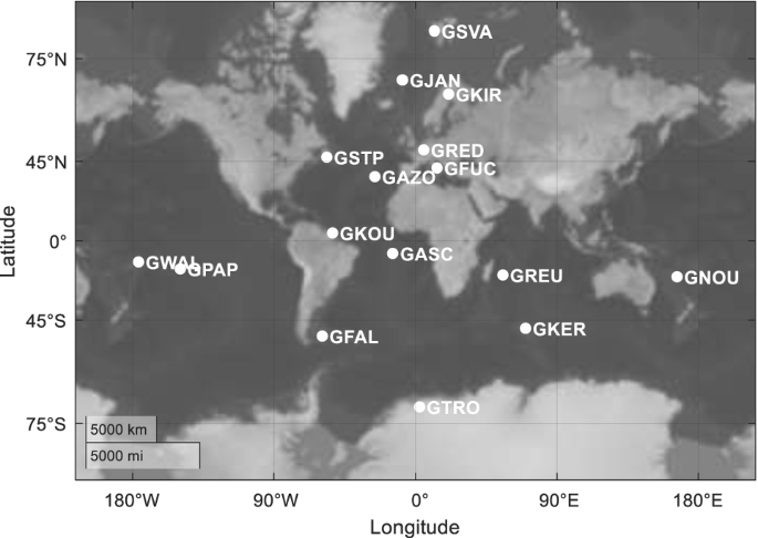
The Galileo Sensor Station network used in this study

3.2 Simulation
The OTWL observations are two-way continuous wave laser ranges as well as clock differences. The measurement errors used to simulate laser observations are given in Table 2. A more detailed description and equations of the errors can be found in Schlicht et al. (2020). To be congruent with the OTWL observations, the sampling rate of the GNSS and OISL observations is 60 seconds as well. The GNSS observations were simulated as dual frequency code and phase measurement for E1 and E5. Effects due to the ionosphere were eliminated to a great extent by forming the ionosphere free linear combination. A summary of the simulated microwave link measurement errors is shown in Table 3. The OISL laser technology is based on EDRS (European Data Relay Satellites) data transfer links. We generated the observation schedule for an any-to-any scenario with bidirectional links between the satellites. Schlicht et al. (2020) show that this scenario offers the best results. The OISL observation schedule was derived from the connectivity scheme by Fernández (2011). We simulated two-way range measurements and clock differences. For the OISL measurements we simulated the errors analogously to the OTWL observations but without troposphere delay errors. This is an advantage for OISL observations as no signal path is disturbed by the troposphere. The measurement errors for OISL are collected in Table 2 as well.
The simulated satellite clocks are hydrogen masers. This leads to a mean satellite clock error of about 24 ns after ten days. Ground station clocks are assumed to be simple quartz oscillators and are simulated based on polynomials of order four with respect to time. The station clock error is smaller than 0.1 µs. Each satellite and each ground station is equipped with one clock, assuming that all observation techniques are connected to the same clock in each satellite and each station. We simulated inter-system biases: a once per revolution variable bias per satellite in case of L-band, emulating a temperature dependency, biases affecting the clock offsets and ranges in case of OISL and biases affecting the clock offsets and ranges in case of OTWL. Hence, each observation technique has its own biases, resulting from different cable lengths and delays on the signal path between the corresponding receiving terminal and the clock. The error free force model in the simulations includes the Earth gravity field up to degree and order 12, ocean and solid Earth tides, influences from third bodies (Sun, Moon, Venus, Mars and Jupiter). For SRP we applied a modeling error (see Sect. 4).
3.3 Estimation
In the solution, we parameterized the satellite orbits with six osculating elements and nine or more empirical SRP parameters (see Sect. 4). Furthermore, we estimated station specific piecewise linear tropospheric zenith delays every two hours (L-band), ground station coordinates per 24 hours (L-band and OTWL), epoch-wise satellite and ground station clocks (L-band, OTWL and OISL) as well as L-band phase ambiguities per pass (float). In addition, we estimated daily range and clock biases for each satellite (OISL and OTWL) as well as each ground station in case of OTWL. We simulated inter-technique biases affecting the clock and the range. However, we estimated only one bias per clock and one per range, representing the bias between L-band and the optical techniques. The estimation of biases per observation technique would be the next step, but is only relevant for the scenarios L-band + OTWL + OISL and OTWL + OISL. Regarding the ground station coordinates, we assumed small coordinate eccentricities errors of about 0.5 mm (3D) between L-band and OTWL. However, we estimate only one reference coordinate per station, to which all observation techniques refer to. An overview of the estimated parameters regarding each observation technique can be found in Table 4. Following the OTWL observation schedule, for 16 ground stations and 24 satellites around 42560 OTWL observations were simulated per day. In comparison, around 403890 GNSS observations in code and phase as well as around 32300 OISL observations were simulated per day.
In the analysis procedure we defined the geodetic datum by fixing the coordinates and the clock of one ground station (GASC) for L-band and OTWL. For comparison, we performed a second procedure fixing another station (GKOU). The analysis shows that fixing another station does not affect the behavior of the results.
Having only 16 ground stations in the estimation, an all-stations-fixed scenario would be chosen in the real world to stabilize the solution since the coordinates are assumed as well known. For this reason, we did another analysis with fixing all 16 ground station coordinates in the estimation (shown at the end of Sect. 5)—still only one ground station clock is fixed. In a first scenario we did not assume station coordinate errors. A second scenario takes station coordinate errors into account. A comparison of both scenarios shows the impact of the coordinate errors on the orbit solution. Defining an all-stations-fixed geodetic datum, the additional constraints added may on the one hand stabilize the solution due to the strong tie to the reference frame, and on the other hand they may distort the solution as systematic errors can no longer be absorbed in the station coordinates. The results in this paper show that a L-band + OISL scenario benefits a lot from an all-stations-fixed geodetic datum, while for a L-band + OTWL scenario the orbits can be adjusted with high accuracy in a system with a one-station-fixed or an all-stations-fixed geodetic datum.
4 Solar radiation pressure modeling
Doing simulations, one faces two typical problems: First, one can only take already known modeling or systematic measurement errors into account. Second, the analysis is future oriented and, hence, it is difficult to specify the utmost precision and accuracy of the measurements. In this study, the main modeling issue in orbit determination of Galileo satellites is SRP. We just focus on this modeling error. Furthermore, we assume a moderate accuracy and precision for the optical ranging techniques. Other non-gravitational forces, like thermal radiation, radiators, thruster leakage and attitude biases, can be taken into account in future work.
Two strategies are possible when modeling SRP:
-
The physical approach is to describe the absorption and reflection properties of the main surfaces of the satellite. For instance, a box-wing model is a physical model that approximates the general shape of the satellite (Bury et al. 2019; Duan et al. 2019).
-
The empirical approach is to estimate periodic accelerations of the satellite in an appropriate coordinate system, described by models like the Empirical CODE Orbit Model 2 (ECOM2) (Arnold et al. 2015).
ECOM2 (see Eq. (1)) is one of the commonly used empirical SRP models in the IGS community for the processing of GNSS solutions. Generally, the SRP parameters are estimated in the Sun-Satellite-Earth frame (SSE): D points from the satellite to the Sun, Y is in the direction along the solar panels and B completes the right-handed orthogonal system. The accelerations in each of the DYB directions encompass a constant term as well as sine and cosine terms with selected frequencies that are integer multiples of once per revolution. ECOM2 covers constant terms in all DYB directions, as well as two and four times per revolution terms in D direction and a once per revolution term in B direction (see Eq. (1) with the argument of latitude with respect to the sun Δu). The per revolution parameters are divided into a sine and cosine parameter. In the further context, we name the parameters related to the direction with the corresponding letter D, Y or B and append the per revolution term by its number. For example, the D2 parameters are related to direction D with a frequency of twice per revolution. A subscript c names the cosine, s the sine parameter and 0 the constant parameters.
Two SRP model types following different modeling strategies is an appropriate starting point for orbit determination simulations:
-
We can define the simulation truth (true orbit) with a physical model.
-
We introduce a slightly wrong physical model representing the a priori modeling error (mismodeled orbit), used as input for the orbit adjustment.
-
Fitting empirical accelerations to realistic measurements with observation errors using a least-squares adjustment results in an adjusted orbit. As the empirical parameters cannot compensate the modeling errors perfectly in total, the adjusted orbit includes a corresponding a posteriori modeling error.
-
Calculating a best possible orbit, we can quantify this a posteriori modeling error (see below).
Hence, this procedure defines four different orbit types that are generally relevant in a simulation study: true, mismodeled, adjusted and best possible orbits. Figure 2 gives a scheme how these orbit types are generated in our study. The following subsections describe the generation of the orbits by guiding through the scheme (Fig. 2), followed by an analysis of the introduced modeling error.

Scheme of the orbit generation procedure of this simulation study
4.1 True orbit
To get as realistic Galileo orbits as possible, we retrieved MGEX CODE orbits of the IGS (Prange et al. 2020) and adjusted them with models. To get the simulation truth for our study, we used the box-wing model by Duan et al. (2019) as a physical model. The box-wing model considers the surfaces of a satellite in ±x, ±y and ±z body-fixed directions (box) and the solar panel area (wings). The physical optical parameters of absorbed α, reflected ρ and diffusely reflected δ photons are modeled for each satellite surface. Integrating the Galileo orbits with a box-wing parameter set assumed as true leads us to the simulation truth, represented by the true orbit that is used to simulate the observations. The FOC and IOV satellites are integrated with slightly different box-wing parameters.
4.2 Mismodeled orbit
To get the mismodeled orbit, the input orbit for the least-squares adjustment, the true orbit was integrated with a modified box-wing parameter set to introduce an orbit with an a priori modeling error. We generated two mismodeled orbits with different SRP modeling errors to analyze the influence of different modeling errors to the solution. The following models are identically used for FOC and IOV satellites, which leads to a slightly higher modeling error for the IOV satellites as the true box-wing parameters have a slightly larger difference.
First, we modified the three optical parameters of absorbed α, reflected ρ and diffusely reflected δ photons in the directions ±x, ±y and ±z by 10–20% (see the equations shown in Table 5). Box surfaces and solar panel sizes remained unchanged. Thus, generated mismodeled orbits are wrong by around 15 cm on average (true—mismodeled orbit). We further call this the mismodeled orbit according to modeling error 1. This mismodeled orbit was mainly used in this simulation study.
Second, we modified the box surface in ±x direction by +4% (Table 6). The solar panel sizes as well as the three optical parameters remained unchanged for all directions for this simulation. We further call this the mismodeled orbit according to modeling error 2.
The satellite producer and ESA do not publish errors for the physical optical parameters, but discussed uncertainties are at a level of about 10%. A study analyzed the error of a box-wing model compared to a CAD (Computer-Aided Design) model and concluded that the satellite surfaces are wrong by 7% for GPS and 2% for Galileo on average for all beta angles (Li and Ziebart 2020). As we analyzed individual errors for the physical optical parameters and the satellite box, our assumed modeling errors fit well to the total acceleration errors due to SRP.
4.3 Adjusted orbit
The resulting orbit from the least-squares adjustment of the measurements is the adjusted orbit. Using the mismodeled orbit as the a priori orbit, the adjusted orbit is based on modeling error 1 or 2, respectively, with additionally adjusted empirical parameters.
4.4 Best possible orbit
The best possible orbit delivers the maximum achievable accuracy from the introduced modeling errors. This orbit is retrieved by adjusting the true orbit positions using an orbit model based on the mismodeled box-wing parameter set and additionally adjusting empirical parameters. The difference of the best possible orbit and the adjusted orbit thus is the fact that the former is adjusted to the true orbit positions while the latter is adjusted to the observations simulated using the true orbit. In comparison with the mismodeled orbit, empirical parameters are estimated for both of them.
4.5 Modeling error analysis
Empirical orbit models like ECOM2 (Eq. (1)) use different per revolution-dependent terms. In a pre-simulation analysis, we investigated the influence of such once per revolution-dependent terms and their multiples, caused by the a priori box-wing model errors. We extracted the computed SRP accelerations from the true and the mismodeled orbit in the SSE frame and computed the differences (true—mismodel). We processed SRP accelerations for the same four 10-day time periods used in the simulation study. The analysis was done for one satellite of each of the four Galileo planes A-D as the beta angle is the same for all satellites in the same orbital plane. The planes A-C refer to the regular Galileo orbital planes. Plane D was defined for the satellites E14 and E18 in eccentric orbits.
Figure 3 shows the Power Spectral Density (PSD) of the acceleration difference true—mismodeled according to modeling error 1 (Table 5) for the days 043–052 from 2019 (19043-052). The following discussion is transferable to the other three simulation time periods as well. In Y direction there is overall no influence. The even per revolution terms are dominant in D direction, while the odd terms are dominant in B direction, as expected. This is less obvious for the satellites E14 and E18 in eccentric orbits for which additional harmonic terms are required because Δu is no longer linear with time. For some beta angles, the three times per revolution term is more dominant than the once per revolution term. Figure 4 shows the PSD of the acceleration difference true—mismodeled according to modeling error 2 (Table 6) for the period 19043-052. The results are again transferable to the other three time periods. In this case, the main terms are up to twice per revolution for all planes. The influence of higher per revolution terms is negligibly small.

PSD of the acceleration difference extracted from the true and mismodeled box-wing model for the time period 19,043–052 with respect to modeling error 1 (Table 5). The results are computed for one satellite of each of the four Galileo planes. Satellite E24 relates to plane A, E12 to B, E04 to C. For the more eccentric satellites like E14 we define the plane D as the fourth plane. The x-axis shows the per revolution terms, the y-axis the amplitude of the acceleration

PSD of the acceleration difference extracted from the true and mismodeled orbit for the time period 19,043–052 with respect to modeling error 2 (Table 6). The x-axis shows the per revolution terms, the y-axis the amplitude of the acceleration. Satellite E24 relates to plane A, E12 to B, E04 to C. For the satellites in eccentric orbits, like E14, we define the plane D as the fourth plane
From this analysis we can conclude that the influence of certain per revolution terms is dependent on different modeling errors and the resulting impact on SRP accelerations. The ECOM2 model was developed by reviewing direct SRP models for GNSS satellites (Arnold et al. 2015). We analyzed the SRP influence by modifying box-wing parameters. In case of a SRP influence with respect to the modeling error 1 (Table 5), we identify in addition to B1, D2 and D4 also a strong influence of B3 parameters, which are not taken into account by the ECOM2 model. In this regard, we would expect an effect on the orbit adjustment with the estimation of additional B3 parameters as well. We mainly use the mismodeled orbit according to modeling error 1 (Table 5) in this simulation study. However, for the discussion of the results in Sect. 5, we compared the adjusted orbits resulting from both mismodeled box-wing models—according to modeling error 1 (Table 5) and modeling error 2 (Table 6)—to show if it is possible to estimate higher per revolution terms to improve the adjusted orbit, independently from the accelerations acting on the satellite.
Furthermore, we analyzed the beta angle dependence of the estimated B as well as the D acceleration parameters for all four analysis periods and all 24 satellites of the constellation. The parameters—sine and cosine of B1, B3 and B5 as well as D2, D4 and D6—which are estimated when generating the best possible orbit, show which of the individual SRP parameters absorb the introduced modeling error 1 (Table 5). Figure 5 shows the absolute value of the obtained empirical accelerations as a function of the beta angle. Generally, in the sine terms no significant beta angle dependence can be found. This is expected as the accelerations from the box-wing model are symmetric with respect to the satellite position along the orbit relative to the Sun. However, in the cosine parameters a clear beta angle dependency is recognizable. The impact on B1 and B3 is relatively large, while for B5 the accelerations are negligibly small for beta angles larger than 40°. Beta angle dependence can be found for D2 and D4 parameters as well. The acceleration related to D6 are, however, relatively small for all beta angles compared to D2, D4 and the B parameters. These results show the varying projection of the accelerations induced by the box-wing modeling error into the SSE coordinate directions as a function of the beta angle.

Dependence of the B1, B3, B5 parameters (top and bottom left graphics) and D2, D4, D6 (top and bottom right graphics) with respect to the beta angle. The analysis was done for the four time periods 19,043–052, 19,012–111, 19,132–141 and 19,163–172 and 24 Galileo satellites. The top graphics show the absolute value of the cosine parameters, the bottom graphics the sine parameters
Furthermore, we had a look at the error of the best possible orbits resulting from the different SRP parameter estimates. When estimating per revolution terms in B and D directions up to order five in the orbit adjustment, a decrease of the mean 3D-RMS orbit error could be determined. When estimating the terms D6, no improvement was recognizable. In a scenario with ECOM2 and estimating terms B3+B5+D6, the best possible mean 3D-RMS error even increased again. For this reason, we investigated in the following only the influence of up to five times per revolution terms. We defined four SRP scenarios for this simulation study: the first scenario relates to the commonly used ECOM2 model given in Eq. (1), in the second we replaced the B1 parameters with B3, see Eq. (2), in the third we extended ECOM2 by B3, Eq. (3), and in the fourth we extended ECOM2 by B3 and B5, Eq. (4).
Figure 6 shows the error of the best possible orbit as a function of the beta angle for the four SRP estimation scenarios. The mean orbit error results in 3.4 mm for scenario (1), 7.0 mm for (2), 1.0 mm for (3) and 0.9 mm for (4). The large mean error for scenario (2) is due to a continuously increasing error for increasing beta angles above 30°. This result is consistent to the result presented in Fig. 5. The course of the polynomial fit of scenario (2) shown in Fig. 6 is similar to the accelerations represented by the cosine B1 in Fig. 5, which is not estimated in scenario (2). The same is recognizable for scenario (1) in Fig. 6 and the accelerations of B3 in Fig. 5. In scenario (3) shown in Fig. 6 both B1 and B3 were estimated, resulting in orbit errors in the range of around 1 mm for all beta angles, showing the importance of estimating these terms. It should be noted that the three IOV satellites (two in plane B and one in C) show slightly larger discrepancies from the mean value, due to the slightly larger simulated SRP modeling error (see Sects. 3.1 and 3.2). However, we have to consider that the overall orbit error is already quite small with maximum values up to around 2.5 mm. The two satellites in eccentric orbits (plane D), however, fit very well with the mean value, although the argument of latitude is not optimal as argument of the harmonic expansion of the SRP accelerations for these satellites. When we compare scenario (4) with (3), a decrease of the orbit errors for small beta angle is recognizable. This behavior coincides with that of the B5 accelerations of Fig. 5. Comparing Fig. 5 and 6, the residuals of the best possible orbit fit show the signature of the not estimated parameter.

Orbit errors of the best possible orbit with respect to the beta angle. The top left figure relates to the SRP modeling according to Eq. (1), the top right to Eq. (2), the bottom left to Eq. (3) and the bottom right to Eq. (4). The black line is a polynomial fit of the data with order five to guide the eyes. The planes A to C are the three regular Galileo satellite planes. Plane D consists of the more eccentric E14 and E18 satellites. The IOV satellites have slightly larger orbit errors regarding the mean value, due to the slightly larger modeling error
5 Results
We now discuss the results of this simulation study. We evaluate the influence of a combined Galileo L-band and OTWL (Optical Two-Way Links) scenario for Galileo POD using 16 Galileo Sensor Stations. The results are compared to an L-band-only scenario. Furthermore, we compare the influence of OTWL in contrast to OISL (Optical Inter-Satellite Link) measurements in addition to Galileo L-band. We evaluate the full network with L-band, OTWL and OISL observations as well as a solution without L-band, making only use of both optical observation techniques. For all observation technique combinations, we additionally show the influence of a B3 SRP parameter estimated in addition to the regular ECOM2 parameter set. Therefore, we compare four scenarios with SRP modeling according to Eqs. (1), (2), (3) and (4). We further also call these the scenarios (1), (2), (3) and (4). The following results were computed using the mismodeled orbit based on modeling error 1 (Table 5). Comparisons to the results generated using mismodeled orbits according to modeling error 2 (Table 6) are added to the discussion.
With two or more different observation techniques in combination, the weighting of the different measurements can significantly affect the results. To find the weights which best represent the real-world observation precision is a critical task. Table 7 collects the weighting (variance factor) for the different analysis scenarios. In this simulation study, we weighted L-band, OTWL and OISL in each combination such that the resulting difference of the true and adjusted orbit is minimized. The result shows that in case of L-band + OTWL and L-band + OISL the L-band phase measurements have to be down-weighted with respect to the more precise OTWL and OISL measurements. In the L-band + OTWL + OISL scenario a different weight leads to negligible differences in the results. Therefore, we weighted L-band, OTWL and OISL equally. For the OTWL + OISL scenario we weighted OISL measurements with respect to the OTWL measurements. In this case, the measurements have to be weighted equally. This is expected since both links have similar systematic errors.
Our analysis encompasses the following four parts:
-
In a first analysis we compare the formal orbit uncertainties. These represent the stochastic measurement errors as well as the observation geometry. We took the information from the covariance matrix of the adjusted orbit parameters propagated in radial, along- and cross-track directions and averaged along the orbit.
-
Second, we analyze the orbit differences between the true and adjusted obits in contrast to the formal orbit uncertainties. The orbit differences include the effects of the systematic modeling errors on the orbits. The analysis of both formal orbit uncertainties and orbit errors was done for solutions based on 16 Galileo Sensor Stations, with coordinates of just one ground station fixed.
-
In a third analysis step, we gradually reduce the number of ground stations for OTWL observations to simulate possible cloudy weather conditions or a Galileo Sensor Station network which is not fully equipped with optical terminals. In this regard, ground stations tracking Galileo L-band signals are not reduced.
-
The fourth analysis step compares the results of solutions with coordinates of just one ground station fixed—for both L-band and OTWL—and with all 16 stations fixed. In doing so, we analyze a first scenario in which no ground station coordinate errors are assumed. In a second scenario, we use wrong coordinates for the simulation of L-band and OTWL observation, with small eccentricity errors between L-band and OTWL. We evaluate the impact of the station coordinate errors on the orbit solutions.
5.1 Formal orbit uncertainty
The formal orbit uncertainty focuses the analysis on the stochastic errors and the geometrical configuration of the measurements. Figure 7 gives the formal orbit uncertainty of all four SRP modeling scenarios for L-band with respect to the beta angle. Shown are the daily mean formal orbit uncertainties per satellite, adjusted by a polynomial of fifth order. No beta angle dependence can be found for the SRP scenarios (1) and (2). However, the scenarios (3) and (4) show a strong increase of the formal orbit uncertainty for beta angles below 15°. Interestingly, for L-band the lowest formal orbit uncertainty of around 27 mm is achievable with SRP scenario (2). This means that this SRP model performs better for our orbit modeling error than the commonly used ECOM2 model with a mean formal orbit uncertainty of around 31 mm. We noticed this behavior already in Schlicht et al. (2020). Estimation of more than nine empirical parameters leads to larger formal orbit errors in an L-band-only solution, compared to the nine parameter models. The mean formal orbit uncertainty is at around 36 mm for scenario (3) and 38 mm for scenario (4). Table 8 collects the simulated scenarios for combined observation technique solutions.

The given formal orbit uncertainty is a 3D mean over the four simulation time periods since no significant beta angle dependence was noticeable for these cases. With L-band + OISL formal uncertainties down to 2.4 mm and with L-band + OTWL down to 0.8 mm are achievable. While for L-band + OISL the best result can be achieved with SRP model (1), model (2) is at the lower end. For L-band + OTWL it is opposite. With a formal orbit uncertainty of around 1.1 mm, the L-band + OTWL + OISL scenario achieves slightly worse results compared to L-band + OTWL. The combination of the optical techniques OTWL + OISL reaches 0.3 mm and represents the best scenario. Overall, the formal orbit uncertainty improvement with respect to the best L-band-only solution is at around 91% for L-band + OISL, around 96 % for L-band + OTWL + OISL, around 97 % for L-band + OTWL and around 99 % for OTWL + OISL. Using the mismodeled orbit according to modeling error 2 (Table 6) gives the same results.
5.2 Orbit error
The analysis of the orbit errors, the difference between the true and adjusted orbits, focuses on the systematic effects in the measurements. In this regard, modeling errors gain importance as well. Figure 8 collects the results for the four SRP models for the L-band-only solution as a function of the beta angle. The results are polynomial adjustments of order five of the daily mean 3D-RMS orbit errors per satellite. The results for the different SRP model solutions resemble the formal orbit uncertainties. Again, with a mean 3D-RMS of around 217 mm, the SRP model (2) gives the best results. In comparison, with ECOM2 a mean orbit error of around 235 mm can be achieved. The main impact of the systematic errors on the POD with L-band is from phase center variations (PCV) errors, which are also intended to cover multipath in our simulations. The error contribution of the PCV is larger than the troposphere delay error, which can be compensated well by estimating station specific piecewise linear tropospheric zenith delays (see Table 4).

Table 9 collects the 3D-RMS orbit errors as a mean of the 40 days of the analysis periods. Figures 9, 10 and 11 give an overview of the 3D-RMS orbit errors as a function of the beta angle for the observation technique combinations. The results regarding SRP modeling according to Eq. (4) are not shown since they are not significantly different from (3).

Orbit errors (3D-RMS) of the solutions related to the different observation technique combinations with respect to the beta angle. The comparison is for SRP modeling according to Eq. (1). The black lines are polynomial adjustments of order five of the daily mean per satellite to guide the eyes

Orbit errors (3D-RMS) of the solutions related to the different observation technique combinations with respect to the beta angle. The comparison is for SRP modeling according to Eq. (2). The black lines are polynomial adjustments of order five of the daily mean per satellite to guide the eyes

Orbit errors (3D-RMS) of the solutions related to the different observation technique combinations with respect to the beta angle. The comparison is for SRP modeling according to Eq. (3). The black lines are polynomial adjustments of order five of the daily mean per satellite to guide the eyes
Figure 9 relates to SRP scenario (1). For the L-band + OTWL scenario a beta angle dependency is recognizable, while the other observation technique combinations do not show a significant beta angle dependence. In analogy to the analysis regarding the best possible orbits (see Fig. 6), the shape of the polynomial adjustment is comparable to the B3 acceleration in Fig. 5 suggesting that it is caused by the not estimated B3 parameters in case (1). The orbit errors for the L-band + OTWL scenario are generally lower than for L-band + OISL, while L-band + OTWL + OISL achieves the best results (see Table 9). The noise in the L-band + OTWL + OISL scenario is extremely small compared to the other combinations. However, still small systematic discrepancies are visible for some satellites at certain times in this case. In the other three scenarios such systematic effects disappear in the noise. The OTWL + OISL scenario overall achieves better results than the L-band + OISL scenario. This means that OTWL can fix the satellite constellation to the solid Earth more effectively than L-band, despite the smaller number of observations per epoch.
For the L-band + OTWL solution with the SRP modeling according to Eq. (2), shown in Fig. 10, an identical behavior is noticeable: the shape of the polynomial adjustment is similar to the B1 accelerations in Fig. 5. In case of scenario (2), the other observation technique combinations show beta angle dependences as well. The L-band + OISL scenario has the weakest beta angle dependency. The influence of not estimated B1 parameters on the results is in total much larger than for not estimated B3 parameters. The achievable orbit quality with L-band + OTWL is again generally superior to L-band + OISL (see Table 9). L-band + OTWL + OISL is still the best scenario, but much closer to the results from L-band + OTWL.
From the analysis to this point it can be concluded that the orbit accuracy related to the OTWL is highly beta angle dependent due to the not estimated SRP parameters B1 or B3. However, when both B1 and B3 parameters are estimated (see Fig. 11), the beta angle dependence disappears. In this case, the other scenarios again do not show this either. This SRP scenario is overall the best for all observation technique combinations. Looking at Table 9, with a mean orbit error of around 3.6 mm, the L-band + OTWL scenario is similar to the L-band + OTWL + OISL scenario (3.4 mm). In this regard, the influence of additional OISL observations would be negligibly small. The orbit error improvement with L-band + OTWL is around 83 % with regard to L-band + OISL and around 98 % with regard to the best L-band-only solution (SRP scenario (2)). The advantage of the ground-space link, in contrast to a satellite-to-satellite link, comes from the possibility to synchronize the ground station clock as well. With OISL, only the satellite clocks are synchronized. Furthermore, the high-precision ground-space oriented OTWL helps with the orbit adjustment in a system with a one-station-fixed geodetic datum (coordinates and clock of just one ground station fixed). As already mentioned, the purely optical scenario OTWL + OISL generally achieves better results than L-band + OISL. However, the good results from the formal orbit uncertainty do not transfer to the orbit error solution. This means that the systematic effects and clock errors cannot be mitigated completely in the OTWL + OISL scenario. The L-band measurements are supportive in this case (see L-band + OTWL + OISL scenario). When we compare these results with the results using the mismodeled orbits according to modeling error 2 (Table 6), the general behavior is the same. These results are summarized in Table 10. The scenario estimating B1 and B3 (SRP scenario (3)) does not negatively affect the results, compared to an estimation with ECOM2 (SRP scenario (1)). Rather, the combinations L-band + OTWL and L-band + OISL show a slight improvement of the 3D-RMS orbit error. This means that all parameters of the SRP scenario (3) with both parameters B1 and B3 could be estimated in an analysis based on these observation technique combinations—independent of the SRP accelerations acting on the satellites.
5.3 Reduced station scenarios for OTWL observations
The reduction in the number of ground stations with OTWL observations simulates possible cloudy weather conditions or a Galileo Sensor Station network which is not fully equipped with optical terminals. However, this analysis also identifies the number of ground stations required to achieve a certain level of orbit improvement with respect to the L-band-only scenario. The number of OTWL ground stations is gradually reduced. Table 11 shows the selected stations for the different scenarios. Figure 12 collects the relative improvement of the orbit error with respect to the L-band-only solution. The shown orbit error improvements are related to the SRP modeling according to Eq. (1), but the behavior is similar for the other SRP modeling scenarios as well. The number of ground stations used for L-band measurements is not reduced in all cases. This means that the result for the L-band + OISL scenario stays unchanged and is just shown for comparison. The L-band + OISL scenario gives a maximum orbit error improvement of around 89% with respect to the L-band-only scenario.

Relative orbit error improvement with respect to the L-band-only scenario in percent. The x-axis displays the number of used OTWL ground stations for each scenario (compare with Table 11). Stations for L-band measurements are unchanged and use the full 16 Galileo Sensor Station network. The results are related to the SRP modeling according to Eq. (1)
Reducing the number of stations in an L-band + OTWL scenario, the orbit error improvement decreases continuously. However, the L-band + OTWL orbit error improvement is superior to the L-band + OISL scenario using more than five OTWL stations. Using three OTWL stations, an orbit error improvement of around 74% is possible and still around 31% with one station, with respect to L-band-only.
It is highly remarkable that the results for the L-band + OTWL + OISL scenario do not significantly change when reducing OTWL observation stations. The orbit error improvement remains constant at around 97.5 % with respect to L-band-only. This means that additional OTWL observations from only a single ground station already give a further orbit error improvement of around 8.5 % with respect to the L-band + OISL scenario. It is very important to note that this one ground station has fixed coordinates and clocks. Signal biases and modeling errors are simulated for the OTWL observations with regard to this fixed station.
In a scenario without L-band, just using OTWL + OISL observations, the orbit error improvement varies slightly with a reduction of the number of ground stations. This is a reminder that the simulation is built on different types of random errors.
5.4 Fixing the ground station coordinates
In a further analysis we compare the results with fixing the coordinates of just one station (GASC) in the estimation, as for the results presented above, and the scenario with fixing the coordinates of all 16 Galileo Sensor Stations for L-band and OTWL. The clocks of the stations, except for one station (GASC), were estimated in any case. Such a scenario also represents a real-world application since the coordinates of grounds stations are generally assumed as well known.
Table 12 shows the results for the scenario with fixed station coordinates for the whole Galileo Sensor Station network of 16 stations. We used no ground station coordinate errors in this scenario. Comparing Table 12 with Table 9, the orbit errors from the L-band-only (1), (3) and (4) scenarios are worse compared to the results of the one-station-fixed scenarios due to station-related modeling errors. As we do not estimate a bias for L-band, all systematic errors are shifted to the station coordinates, clocks or the orbits. When all stations are fixed, we remove some of the freedoms for the least-squares adjustment. Again scenario (2) is the best and, interestingly, is the only scenario which improves compared to the one-station-fixed scenario (see Table 9). A large improvement can be achieved for L-band + OISL for all SRP modeling scenarios. Especially the scenarios with more than 9 SRP parameters estimated ((3) and (4)) profit from the fixing. This improvement for OISL is due to the strong tie of the constellation to the solid Earth in an all-stations-fixed reference frame. With just one fixed station, the satellite constellation has more degrees of freedom in the adjustment to the OISL observations. The fixing of all coordinates, however, ties the orbits to the solid Earth at multiple sites. The L-band + OTWL scenario shows slightly worse results with a fixed station network, comparing the best SRP scenario (3) in Tables 9 and 12. Nevertheless, the 3D-RMS orbit error is still smaller than for the L-band + OISL scenario. Both the L-band + OTWL + OISL and the OTWL + OISL scenarios profit from the all-stations-fixed geodetic datum. In case of the scenarios (3) and (4), L-band + OISL is superior to OTWL + OISL in this all-stations-fixed scenario.
To get the results shown in Table 13 we again fixed all station coordinates in the estimation process, but in this scenario we included station coordinate errors for the measurements simulation, based the coordinate accuracies provided by the ITRF. The 3D station coordinate errors for L-band are 1.1 mm on average. For OTWL observations we assumed small eccentricity errors to L-band up to about 0.5 mm per station in 3D. The resulting 3D station coordinate errors for OTWL are 1.2 mm on average. The analysis shows the impact of errors in the station coordinates on the orbit solutions. In the L-band-only scenario, the wrong station coordinates affect the orbit solution by up to 0.5 mm. Analyzing L-band + OTWL, the scenarios with a SRP modeling error according to Eqs. (1) and (2) are only affected by 0.3 mm, while scenarios with an estimation of more than 9 SRP parameters (scenario (3) and (4)) are affected by up to 0.9 mm. This is almost the full 3D station coordinate error. In contrast, scenarios including OISL measurements are not influenced by using wrong station coordinates instead of the true coordinates in the simulation. The satellites themselves are tied to each other by the OISL observations as well as tied to the solid Earth at multiple sites by fixing the station coordinates. For these reasons, small station coordinate errors average out for scenarios with OISL, similar to the comparatively large systematic errors of L-band.
6 Conclusions and outlook
In this simulation study we have analyzed the impact of ground-space optical two-way links for Galileo precise orbit determination. The optical two-way link (OTWL) observations are in addition to L-band measurements. The L-band and OTWL observations were simulated with regard to 16 Galileo Sensor Stations. We compared the L-band + OTWL solution to a solution with optical inter-satellite links (OISL) (L-band + OISL). We further analyzed the observation technique combinations L-band + OTWL + OISL and the optical-only OTWL + OISL scenario. We performed an analysis regarding the estimation of additional solar radiation parameters in these scenarios. Many systematic effects were taken into account: link biases and their variability, distance-dependent effects, colored noise and a troposphere error for OTWL measurements. We simulated inter-technique clock biases while estimating only one bias for each clock.
We can conclude that the Galileo processing can highly benefit from the use of additional OTWL measurements. The improvements in the orbit solution using L-band + OTWL observations can be attributed to the two main advantages of OTWL compared to L-band measurements. First the higher ranging accuracy and precision. This helps for a better compensation of systematic errors. Second, the two-way link gives the possibility to synchronize the station and satellite clock. We did not study the influence of the clock synchronization on the orbit determination in this paper, but analyzed it in Schlicht et al. (2019). The impact of the clock synchronization is small compared to the impact of the range measurements.
From the results of this work, the following conclusions can be drawn for OTWL:
-
The high-precision ground-space oriented links help with the orbit adjustment of a system with a one-station-fixed geodetic datum. This is due to the tie of the satellite constellation to the terrestrial reference frame through the high-precision ground-space links and the additional synchronization of the ground clocks.
-
OTWL is dependent on the number of available ground stations. In case that less than seven ground stations are available for OTWL observations, while the other stations are restricted, for instance due to cloudy weather conditions, the L-band + OISL solution achieves smaller three-dimensional (3D)—root mean square (RMS) orbit error results than L-band + OTWL.
-
A L-band + OTWL scenario cannot profit from the ground station coordinate fixing (all-stations-fixed geodetic datum) anymore as the L-band systematic errors are already compensated to a great extent by OTWL.
-
Applying in addition station coordinate errors, only scenarios using L-band + OTWL and with estimation of more than nine solar radiation pressure (SRP) parameters have a significant relative increase of the orbit error. The impact on the 3D-RMS orbit error is about 0.9 mm, starting from an a priori 3D station coordinate error of about 1.2 mm on average.
For OISL, the following conclusions can be drawn:
-
In a system with a one-station-fixed geodetic datum, the resulting orbit error from L-band + OISL is six times worse compared to the solution from L-band + OTWL. The reason is that OISL measurements can only constrain the internal geometry of the satellite constellation, while L-band does not provide a strong tying to the solid Earth due to the large systematic errors and the one-way nature of the technique.
-
In a system with an all-stations-fixed geodetic datum, a huge improvement for L-band + OISL can be achieved. This is due to the tying of the satellite constellation to the solid Earth. The orbit error resulting from L-band + OISL is almost at the same level as for L-band + OTWL.
-
Applying in addition station coordinate errors, scenarios including OISL measurements achieved the same results as for the scenario without coordinate errors.
The addition of OISL observations to L-band + OTWL improves the measurement geometry and fixes the internal geometry of the satellite constellation. Generally, this is the best solution, especially in case of less than 16 stations available for OTWL measurements. An optical-only scenario—OTWL + OISL—achieved worse 3D-RMS orbit errors compared to the results from scenarios including L-band and OTWL. This means, L-band is supportive for the OTWL bias estimation.
For the SRP analysis we can conclude that a combination of two or more observation techniques allows the estimation of more than nine orbit modeling parameters. Schlicht et al. (2020) already showed this for an inter-satellite link scenario, we can confirm this for an L-band + OTWL as well as the L-band + OTWL + OISL scenario. For the latter it would have been even possible to estimate 13 empirical parameters—Empirical CODE Orbit Model 2 (ECOM2; Arnold et al. 2015) + B3 + B5. However, there is no further benefit with estimating B5 parameters. Nevertheless, the possibility to estimate more SRP parameters allows a more precise orbit modeling. The overall best results could be achieved for an ECOM2 + B3 parameter model.
With the possibility to get better modeled orbits, the geodetic parameters will not contain signals with a draconitic period. This would be a huge step forward to reach the goals of GGOS (Global Geodetic Observing System; Plag and Pearlman 2009) of a precise terrestrial reference frame with 1 mm accuracy and a stability of 0.1 mm/year as well as improving the precision of the societal and scientific applications of GNSS (Global Navigation Satellite System) (Plag and Pearlman 2009; Johnston et al. 2017).
Furthermore, the combination of different observation techniques is one of the next important steps in improving satellite orbits as well as space geodesy. Especially the combination of OTWL and OISL is of great interest for future application. As previously mentioned, a general advantage of the OTWL concept, in contrast to OISL, is the tight tie to the terrestrial reference frame. Not only the satellite orbits but also both the satellite and ground station clock can be synchronized. From a future aspect, compared to OISL we would expect an improved estimation of Earth Rotation Parameters (ERPs) as well as the possibility to optimize the ITRF (International Terrestrial Reference Frame) with the OTWL measurements due to the tight connection of precise GNSS orbits to the terrestrial frame. Hence, the influence of L-band + OTWL on the ERPs as well as the ITRF is a very interesting question.
We paid considerable attention to the simulation of systematic effects, but of course there are still systematic errors in the orbit determination which were not taken into account in this paper. These errors will be studied in future work, but on the other hand, there is still more potential using a high-precision optical two-way link we did not take into account in our simulations. This is, for example, the calibration of the L-band, which was already shown for T2L2 (Time Transfer by Laser Link; Samain et al. 2014) and GNSS (Leute et al. 2018). The calibration provides great support for the ambiguity resolution with integer ambiguities. Thus, a calibrated L-band can provide support when the optical link cannot operate due to cloudy weather conditions. Furthermore, with the possibility to estimate more parameters in general, a potential for the estimation of other non-gravitational forces, like thruster leakage or radiator properties, can be expected.
The weighting of the different measurement types concerning the L-band measurements in observation technique combinations is a challenging task and may need some more experience: which weights optimally represent the real-world precisions? We weighted the measurement according to the best achievable orbit accuracies as a start. This gives an indication for the potential of the measurement combinations.
In the end it is worth to mention that the synergy to use the same link as a data transfer link is an option that should not be ignored. Such a link can work as a backup or even an alternative to microwave data downlinks. This provides increased security, too, as an optical connection cannot be eavesdropped.
Data availability
All models and assumptions used for the simulation of all observations used in this study are provided in the paper.
References
Abich K, Abramovici A, Amparan B, Baatzsch A, Okihiro BB et al (2019) In-orbit performance of the GRACE follow-on laser ranging interferometer. Phys Rev Lett 123(3):031101. https://doi.org/10.1103/PhysRevLett.123.031101
Arnold D, Meindl M, Beutler G, Dach R, Schaer S, Lutz S, Prange L, Sosnica K, Mervart L, Jäggi A (2015) CODE’s new solar radiation pressure model for GNSS orbit determination. J Geod 89:775–791. https://doi.org/10.1007/s00190-015-0814-4
Boehm J, Werl B, Schuh H (2006a) Troposphere mapping functions for GPS and very long baseline interferometry from European Centre for Medium-Range Weather Forecasts operational analysis data. J Geophys Res 111:B02406. https://doi.org/10.1029/2005JB003629
Boehm J, Niell A, Tregoning P, Schuh H (2006b) Global mapping function (GMF): a new empirical mapping function based on numerical weather model data. Geophys Res Lett 33:L07304. https://doi.org/10.1029/2005GL025546
Boehm J, Heinkelmann R, Schuh H (2007) Short note: a global model of pressure and temperature for geodetic applications. J Geod 81(10):679–683. https://doi.org/10.1007/s00190-007-0135-3
Bury G, Zajdel R, Sośnica K (2019) Accounting for perturbing forces acting on Galileo using a box-wing model. GPS Solut 23:74. https://doi.org/10.1007/s10291-019-0860-0
Bury G, Sośnica K, Zajdel R, Strugarek D, Hugentobler U (2021) Determination of precise Galileo orbits using combined GNSS and SLR observations. GPS Solut 25:11. https://doi.org/10.1007/s10291-020-01045-3
Cacciapuoti L, Salomon Ch (2009) Space clocks and fundamental tests: The ACES experiment. Eur Phys J Spec Top 172(1):57–68. https://doi.org/10.1140/epjst/e2009-01041-7
Cacciapuoti L, Armano M, Much R, Sy O, Helm A, Hess MP, Kehrer J, Koller S, Niedermaier T, Esnault FX, Massonnet D, Goujon D, Pittet J, Rochat P, Liu S, Schaefer W, Schwall T, Prochazka I, Schlicht A, Schreiber U, Delva P, Guerlin C, Laurent P, Le Poncin-Lafitte C, Lilley M, Savalle E, Wolf P, Meynadier F, Salomon C (2020) Testing gravity with cold-atom clocks in space. Eur Phys J D 74:164. https://doi.org/10.1140/epjd/e2020-10167-7
Calzolaio D, Curreli F, Duncan J, Moorhouse A, Perez G, Voegt S (2020) EDRS-C—The second node of the European Data Relay System is in orbit. Acta Astronaut 177:537–544. https://doi.org/10.1016/j.actaastro.2020.07.043
Dach R, Lutz S, Walser P, Fridez P (2015) Bernese GNSS Software Version 5.2. User manual, Astronomical Institute, University of Bern, Bern Open Publishing. ISBN: 978-3-906813-05-9. https://doi.org/10.7892/boris.72297
Delva P, Meynadier F, Wolf P, Le Poncin-Lafitte C, Lauraent P (2012) Time and frequency transfer with a microwave link in the ACES/PHARAO mission. 2012 European Frequency and Time Forum, pp 28–35. https://doi.org/10.1109/EFTF.2012.6502327
Duan B, Hugentobler U, Selmke I (2019) The adjusted optical properties for Galileo/BeiDou-2/QZS-1 satellites and initial results on BeiDou-3e and QZS-2 satellites. Adv Space Res 63(5):1803–1812. https://doi.org/10.1016/j.asr.2018.11.007
Exertier P, Belli A, Samain E, Meng W, Zhang H, Tang K, Schlicht A, Schreiber U, Hugentobler U, Prochazka I, Sun X, McGarry JF, Mao D, Neumann A (2019) Time and laser ranging: a window of opportunity for geodesy, navigation, and metrology. J Geod 93:2389–2404. https://doi.org/10.1007/s00190-018-1173-8
Falcone M, Hahn J, Burger T (2017) Galileo. In: Teunissen PJ, Montenbruck O (eds) Springer handbook of global navigation satellite systems. Springer Handbooks. Springer, Cham. ISBN: 978-3-319-42926-7. https://doi.org/10.1007/978-3-319-42928-1_9
Fernández FA (2011) Inter-satellite ranging and inter-satellite communication links for enhancing GNSS satellite broadcast navigation data. Adv Space Res 47:786–801. https://doi.org/10.1016/j.asr.2010.10.002
Fernández A, Sánchez M, Beck T, Amarillo F (2010) Future satellite navigation system architecture: inter-satellite ranging and orbit determination. In: Proceedings of the 2010 international technical meeting of the institute of navigation, San Diego, CA, pp 872–879
Fliegel HF, Gallini TE, Swift ER (1992) Global positioning system radiation force model for geodetic applications. J Geophys Res 97(B1):559–568. https://doi.org/10.1029/91JB02564
Gill E (1999) Precise GNSS-2 satellite orbit determination based on inter-satellite-links. In: 14th international symposium on space flight mechanics, Iguassu, Brazil
Giorgi G, Schmidt TD, Trainotti C, Mata-Calvo R, Fuchs C, Hoque MM, Berdermann J, Furthner J, Günther C, Schuldt T, Sanjuan J, Gohlke M, Oswald M, Braxmaier C, Balidakis K, Dick G, Flechtner F, Ge M, Glaser S, König R, Michalak G, Murböck M, Semmling M, Schuh H (2019) Advanced technologies for satellite navigation and geodesy. Adv Space Res 64:1256–1273. https://doi.org/10.1016/j.asr.2019.06.010
Hemmati H (2020) Near-Earth laser communications. In: Hemmati H (ed) Near-Earth laser communications, 2nd ed. CRC Press, Boca Raton. ISBN: 978-1-498-77740-7
Hess MP, Stringhetti L, Hummelsberger B, Hausner K, Stalford R, Nasca R, Cacciapuoti L, Much R, Feltham S, Vudali T, Leger B, Picard F, Massonnet D, Rochat P, Goujon D, Schäfer W, Laurent P, Lemonde P, Clairon A, Wolf P, Salomon C, Procházka I, Schreiber U, Montenbruck O (2011) The ACES mission: System development and test status. Acta Astronaut 69:929–938. https://doi.org/10.1016/j.actaastro.2011.07.002
Holmes JK (1990) Coherent spread-spectrum systems. Krieger Publishing Co., FL. ISBN: 978-0-89464-468-9
Johnston G, Riddell A, Hausler G (2017) The international GNSS service. In: Teunissen PJ, Montenbruck O (eds) Springer handbook of global navigation satellite systems. Springer Handbooks. Springer, Cham. ISBN: 978-3-319–42926-7. https://doi.org/10.1007/978-3-319-42928-1_33
Koepf GA, Marshalek RG, Begley DL (2002) Space laser communications: a review of major programs in the United States. Int J Electron Commun 56(4):232–242. https://doi.org/10.1078/1434-8411-54100103
Leute J, Petit G, Exertier P, Samain E, Rovera D, Uhrich P (2018) High accuracy continuous time transfer with GPS IPPP and T2L2. 2018 European Frequency and Time Forum, pp 249–252. https://doi.org/10.1109/EFTF.2018.8409043.
Li Z, Ziebart M (2020) Uncertainty analysis on direct solar radiation pressure modelling for GPS IIR and Galileo FOC satellites. Adv Space Res. https://doi.org/10.1016/j.asr.2020.04.050
Luceri V, Pirri M, Rodríguez J, Appleby G, Pavlis EC, Müller H (2019) Systematic errors in SLR data and their impact on the ILRS products. J Geod 93:2357–2366. https://doi.org/10.1007/s00190-019-01319-w
Marini JW, Murray CW (1973) Correction of laser range tracking data for atmospheric refraction at elevations above 10 degrees. NASA GSFC X-591-73-351.
McNamara P, Vitale S, Danzmann K (on behalf of the LISA Pathfinder Science Working Team 2008) (2008) LISA pathfinder. Class Quant Grav 25(11). https://doi.org/10.1088/0264-9381/25/11/114034.
Mendes VB, Pavlis EC (2004) High-accuracy zenith delay prediction at optical wavelengths. Geophys Res Lett 31:L14602. https://doi.org/10.1029/2004GL020308
Meng W, Zhang H, Huang P, Wang J, Zhang Z, Liao Y, Ye Y, Hu W, Wang Y, Chen W, Yang F, Prochazka I (2013) Design and experiment of onboard laser time transfer in Chinese Beidou navigation satellites. Adv Space Res 51:951–958. https://doi.org/10.1016/j.asr.2012.08.007
Michalak G, Glaser S, Neumayer KH, Koenig R (2021) Precise orbit and Earth parameter determination supported by LEO satellites, inter-satellite links and synchronized clocks of a future GNSS. Adv Space Res. J Pre-proof, Available online 18 March 2021 (in Press). https://doi.org/10.1016/j.asr.2021.03.008.
Montenbruck O, Gill E (2005) Satellite orbits—models, methods, applications. Springer, Berlin, ISBN: 3-540-67280-X.
Plag H-P, Pearlman M (2009) Global geodetic observing system: meeting the requirements of a global society on a changing planet in 2020. Springer, Berlin. https://doi.org/10.1007/978-3-642-02687-4. ISBN: 978-3-642-02686-7.
Prange L, Villiger A, Siderov D, Schaer S, Beutler G, Dach R, Jäggi A (2020) Overview of CODE’s MGEX solution with the focus on Galileo. Adv Space Res 66(12):2786–2798. https://doi.org/10.1016/j.asr.2020.04.038
Pribil K, Hemmati H (2020) Laser transmitters: coherent and direct detection. In: Hemmati H (ed) Near-Earth laser communications, 2nd ed. CRC Press, Boca Raton. ISBN: 978-1-498-77740-7
Prochazka I, Schreiber U, Schäfer W (2011) Laser time transfer and its application in the Galileo programme. Adv Space Res 47(2):239–246. https://doi.org/10.1016/j.asr.2010.02.008
Riley W (2008) Handbook of frequency stability analysis. NIST Special Publications, Boca Raton, p 1065
Samain E, Vrancken P, Guillemot P, Fridelance P, Exertier P (2014) Time transfer by laser link (T2L2): characterization and calibration of the flight instrument. Metrologia 51:503–515. https://doi.org/10.1088/0026-1394/51/5/503
Schlicht A, Hugentobler U, Marz S, Seel S, Biller P (2019) Concept for continuous wave laser ranging and time transfer to Galileo using optical two-way links. In: Proceedings of the 7th international colloquium on scientific and fundamental aspects of GNSS, Zurich
Schlicht A, Marz S, Stetter M, Hugentobler U, Schäfer W (2020) Galileo POD using optical inter-satellite links: a simulation study. Adv Space Res 66(7):1558–1570. https://doi.org/10.1016/j.asr.2020.06.028
Schreiber KU, Kodet, j. (2018) The application of coherent local time for optical time transfer and the quantification of systematic errors in satellite laser ranging. Space Sci Rev 214:22. https://doi.org/10.1007/s11214-017-0457-2
Schreiber KU, Prochazka I, Lauber P, Hugentobler U, Schäfer W, Cacciapuoti L, Nasca R (2010) Ground-based demonstration of the European Laser Timing (ELT) experiment. IEEE Trans Ultrason Ferroelectr Freq Control 57(3):728–737. https://doi.org/10.1109/TUFFC.2010.1471
Shargorodsky VD, Pasynkov VV, Sadovnikov MA, Chubykin AA (2013) Laser glonass: era of extended precision. Glonass Herald J Navig 14:22–26
Sośnica K, Thaller D, Dach R, Steigenberger P, Beutler G, Arnold D, Jäggi A (2015) (2015) Satellite laser ranging to GPS and GLONASS. J Geod 89:725–743. https://doi.org/10.1007/s00190-015-0810-8
Springer TA, Beutler G, Rothacher M (1999) A new solar radiation pressure model for GPS. Adv Space Res 23(4):673–676. https://doi.org/10.1016/S0273-1177(99)00158-1
Thaller D, Dach R, Seitz M, Beutler G, Marayen M, Richter B (2011) Combination of GNSS and SLR observations using satellite co-locations. J Geod 85:257–272. https://doi.org/10.1007/s00190-010-0433-z
Urschl C, Beutler G, Gurtner W, Hugentobler U, Schaer S (2007) Contribution of SLR tracking data to GNSS orbit determination. Adv Space Res 39(10):1515–1523. https://doi.org/10.1016/j.asr.2007.01.038
Weyrauch T, Vorontsov MA (2004) Free-space laser communications with adaptive optics: atmospheric compensation experiments. In: Majumdar AK, Ricklin JC (eds) Free-space laser communications. Optical and fiber communications reports, vol 2. Springer, New York. ISBN: 978-0-387-28652-5. https://doi.org/10.1007/978-0-387-28677-8_5
Zajdel R, Sośnica K, Drożdżewski M, Bury G, Strugarek D (2019) Impact of network constraining on the terrestrial reference frame realization based on SLR observations to LAGEOS. J Geod 93:2293–2313. https://doi.org/10.1007/s00190-019-01307-0
Zech H, Heine F, Tröndle D, Seel S, Motzigemba M, Meyer R, Philipp-May S (2015) LCT for EDRS: LEO to GEO optical communications at 1,8 Gbps between Alphasat and Sentinel 1a. In: Proceedings of SPIE 9647, unmanned/unattended sensors and sensor networks XI; and advanced free-space optical communication techniques and applications, 96470J (29 October 2015). https://doi.org/10.1117/12.2196273.
Zhang H, Cheng Z, Long M, Deng H, Meng W, Wu Z, Zhao G, Zhang Z (2019) Applications of satellite laser ranging and laser time transfer in BeiDou navigation satellite system. Optik 188:251–262. https://doi.org/10.1016/j.ijleo.2019.04.131
Zhang R, Tu R, Zhang P, Fan L, Han J, Lu X (2021) Orbit determination of BDS-3 satellite based on regional ground tracking station and inter-satellite link observations. Adv Space Res Corrected Proof Available online 1 March 2021 (in Press). https://doi.org/10.1016/j.asr.2021.02.027.
Acknowledgements
The German Research Foundation (DFG) is gratefully acknowledged for funding the Project AOBJ:638291.
Funding
Open Access funding enabled and organized by Projekt DEAL.
Author information
Authors and Affiliations
Contributions
SM and AS designed the study. SM performed the data processing, compiled the figures and wrote the paper with the assistance from AS and UH. All authors reviewed the paper.
Corresponding author
Rights and permissions
Open Access This article is licensed under a Creative Commons Attribution 4.0 International License, which permits use, sharing, adaptation, distribution and reproduction in any medium or format, as long as you give appropriate credit to the original author(s) and the source, provide a link to the Creative Commons licence, and indicate if changes were made. The images or other third party material in this article are included in the article's Creative Commons licence, unless indicated otherwise in a credit line to the material. If material is not included in the article's Creative Commons licence and your intended use is not permitted by statutory regulation or exceeds the permitted use, you will need to obtain permission directly from the copyright holder. To view a copy of this licence, visit http://creativecommons.org/licenses/by/4.0/.
About this article

Cite this article
Marz, S., Schlicht, A. & Hugentobler, U. Galileo precise orbit determination with optical two-way links (OTWL): a continuous wave laser ranging and time transfer concept. J Geod 95, 85 (2021). https://doi.org/10.1007/s00190-021-01534-4
Received:
Accepted:
Published:
DOI: https://doi.org/10.1007/s00190-021-01534-4