
Multivariate Analysis of Cryptocurrencies


MEMOTEF Department, Sapienza University of Rome, 00185 Rome, Italy
Econometrics 2021, 9(3), 28; https://doi.org/10.3390/econometrics9030028
Submission received: 17 March 2021
/
Revised: 24 June 2021
/
Accepted: 28 June 2021
/
Published: 1 July 2021
(This article belongs to the Special Issue Topics in Computational Econometrics and Finance: Theory and Applications)
Abstract
:Recently, the world of cryptocurrencies has experienced an undoubted increase in interest. Since the first cryptocurrency appeared in 2009 in the aftermath of the Great Recession, the popularity of digital currencies has, year by year, risen continuously. As of February 2021, there are more than 8525 cryptocurrencies with a market value of approximately USD 1676 billion. These particular assets can be used to diversify the portfolio as well as for speculative actions. For this reason, investigating the daily volatility and co-volatility of cryptocurrencies is crucial for investors and portfolio managers. In this work, the interdependencies among a panel of the most traded digital currencies are explored and evaluated from statistical and economic points of view. Taking advantage of the monthly Google queries (which appear to be the factors driving the price dynamics) on cryptocurrencies, we adopted a mixed-frequency approach within the Dynamic Conditional Correlation (DCC) model. In particular, we introduced the Double Asymmetric GARCH–MIDAS model in the DCC framework.
1. Introduction
During the last few years, interest in the world of cryptocurrencies has exploded, as underlined by the huge rise in Google queries concerning digital currencies. Unlike a standard currency, which is supported by a government or central bank, a digital currency has the feature of allowing online payments linking the giver and the recipient directly, without using a financial institution. The first digital currency, named Bitcoin, dates back to 2008. It was developed in the middle of the Great Recession period based on the paper of Nakamoto (2008). At that time, the stability of the global banking system was highly strained. As pointed out by Weber (2016), Bitcoin took advantage of these circumstances and gained popularity among practitioners, academics, and the financial press. After the European sovereign debt crisis (2010–2013), the confidence in the banking system’s stability sharply reduced. As a consequence, Bitcoin notably rose in value. At present, the diffusion of cryptocurrencies has reached unprecedented levels. The popularity of cryptocurrencies has been underlined by several works. For instance, ElBahrawy et al. (2017) analyzed the statistical properties of the whole cryptocurrency market, Hileman and Rauchs (2017) focused on the cryptocurrency industry and how these digital currencies can be used, and Gandal and Halaburda (2016) investigated the appreciation and depreciation of six different cryptocurrencies.
According to the site https://coinmarketcap.com/ accessed on 30 June 2021, at the time of writing, there were 8525 cryptocurrencies, with a market value of approximately USD 1676 billion. Among all these cryptocurrencies, Bitcoin has the largest market share (around 61%), followed by Ethereum (13%). The reason behind this increasing popularity remains debatable, but probably lies in the heterogeneous nature of digital currencies. In fact, the question of whether cryptocurrencies are a real currency (Yermack 2015), a speculative investment (Baek and Elbeck 2015), a safe haven (Bouri et al. 2017, 2020) or even a general financial asset (Elendner et al. 2018) is still debated. Because of this, investigating the volatility and co-volatility among the cryptocurrencies is crucial and of primary interest for investors and portfolio managers.
Since the seminal paper of Engle (1982), the literature on financial econometrics has focused on volatility modeling and forecasting through the Generalized AutoRegressive Conditional Heteroskedasticity (GARCH) model, surveyed by Teräsvirta (2009). Modeling cryptocurrencies’ volatility using the GARCH specification has become standard among practitioners and scholars. For instance, Chu et al. (2017) analyzed the volatility of seven cryptocurrencies using twelve GARCH specifications; Catania et al. (2018), using GARCH and other models, predicted the volatility of four cryptocurrencies (Bitcoin, Ethereum, Litecoin, and Ripple) and Caporale and Zekokh (2019) used more than one thousand GARCH models for four cryptocurrencies. Taking advantage of the Mixing-Data Sampling (MIDAS) methods (Ghysels et al. 2007), the GARCH–MIDAS (Engle et al. 2013) models have also been used within the cryptocurrency framework. Conrad et al. (2018) investigated Bitcoin’s volatility in detail by including additional macroeconomic and financial variables (observed at a monthly frequency) as potential drivers of the volatility. Walther et al. (2019) used GARCH–MIDAS to forecast the volatility of five cryptocurrencies (Bitcoin, Etherium, Litecoin, Ripple, and Stellar) by including some monthly economic and financial drivers.
Recently, the literature has also been interested in the interdependencies among cryptocurrencies and other financial assets. For instance, Cebrián-Hernández and Jiménez-Rodríguez (2021) used the Dynamic Conditional Correlation (DCC) model of Engle (2002) on a mixed portfolio composed of Bitcoin and ten other assets. Mensi et al. (2020) applied the DCC model to four cryptocurrencies (Bitcoin, Ethereum, Litecoin, and Ripple). Katsiampa et al. (2019) applied the Diagonal BEKK (Engle and Kroner 1995) and its asymmetric version to eight cryptocurrencies. Using a multivariate factor stochastic volatility model in a Bayesian framework, Shi et al. (2020) investigated the dynamic correlations among six cryptocurrencies. García-Medina and Chaudary (2020) studied the interconnections of cryptocurrencies in a network context by estimating the multivariate transfer entropy. Ji et al. (2019) investigated the volatility spillovers among six cryptocurrencies, finding that Bitcoin and Litecoin played a prominent role.
Despite the literature on multivariate analysis of cryptocurrencies is rich, some questions still remain: (i) how to deal with the inclusion of the variables observed at lower frequencies, with a potential separate effect if positive or negative, and influencing daily cryptocurrencies in a multivariate context; (ii) what benefit these variables can give from statistical and economic points of view. The present paper aims to address these points. In particular, the contribution of this work is twofold. First, we analyze the interdependencies among seven cryptocurrencies for the period 2017–2020 by using a set of popular DCC specifications—that is, the corrected DCC (cDCC) of Aielli (2013), the DCC-MIDAS of Colacito et al. (2011), and the Dynamic Equicorrelation (DECO) of Engle and Kelly (2012), as well as a popular non-parametric specification, the RiskMetrics (RM) model, which is also used in Amendola et al. (2020). The DCC class of models is a standard tool for investigating the dynamic interdependencies between financial assets (Hemche et al. 2016). In this paper, the DCC models also include a monthly variable in a context where the dependent variable—that is, the digital currency—is observed daily. The chosen monthly variable is the Google searches of each digital currency. This choice is motivated by Kristoufek (2013), who argued that the Google queries on the digital currencies are the factors determining the cryptocurrencies’ prices. The specification used for including the Google trend data on cryptocurrencies in the univariate specifications is the Double Asymmetric GARCH–MIDAS (DAGM), which was recently proposed by Amendola et al. (2019). The DAGM model is able to take into account the separate effects that positive and negative variations in the low-frequency variable—in this case, the monthly Google searches—may have on the daily (cryptocurrency) volatility. The second contribution of our work is that we evaluate the models from statistical and economic perspectives, as has been done by Amendola and Candila (2017), among others. The statistical evaluation is based on the distance between each predicted conditional covariance matrix and a covariance proxy. The economic evaluation refers to the portfolio Value-at-Risk (VaR) obtained from the global minimum variance (GMV) strategy. As in Elendner et al. (2018), we analyzed a portfolio entirely composed of cryptocurrencies.
The estimation of all the models employed in this work was carried out using the Gaussian distribution. The fat tails and severe skewness are very well-known features of cryptocurrency returns (see, for instance, the works of Bariviera et al. (2017), Zhang et al. (2018), and Näf et al. (2019), among others). The univariate analysis can involve distributions, different from the Normal one, handling efficiently these stylized facts. However, as stated by Pesaran and Pesaran (2010), when the DCC models are estimated using a non-normal distribution, some problems may arise. First of all, there could exist different local maxima. Moreover, the possibility of splitting the estimate stage into two steps is lost. This aspect means that the DCC models’ estimation is problematic, as many parameters have to be optimized jointly. Recently, a viable approach that addresses and solves this issue was proposed in Paolella and Polak (2015) and Paolella et al. (2019). This is accomplished via the use of an expectation–maximization algorithm to jointly estimate all model parameters amid a non-Gaussian distribution. Thus, it is also applicable to high dimensions. We did not pursue this methodology in this paper, leaving it for future work. Instead, we continued to use the Gaussian distribution, because it is the dominant choice in this context (it has been recently used in Canh et al. (2019), Guesmi et al. (2019), and Kumar and Anandarao (2019), for instance).
In terms of results, the inclusion of the monthly Google searches as additional determinants for the daily volatilities of the chosen digital currencies is extremely important. In fact, only the models using Google searches belong to the set of superior models (SSM), identified through the Model Confidence Set (MCS, Hansen et al. 2011) procedure. These results hold both for the statistical and economic evaluations. Moreover, only the models employing the Google trends and the RM model have satisfactory residual diagnostics. Finally, all the estimated time-varying conditional correlations obtained from the models within the SSM are relatively high, approximately ranging between 0.6 and 0.8 in the last part of the sample.
2. Methodology
Let be the vector of n daily log-returns observed at time i of period t. Typically, the frequency of period i is higher than the frequency of t in order to take into account the additional volatility determinants which, in this work, will be observed at a monthly frequency. Globally, there are days within each period t, and there are T low-frequency periods. Then, we assume that:
where is the multivariate normal distribution; is the conditional covariance matrix; is the diagonal matrix, which includes the conditional standard deviations on the main diagonal; and is the correlation matrix, which is formulated as:
In Equation (3), denotes the conditional expectation made at time of the period t. By means of this formulation, are the standardized residuals obtained from the univariate volatility models. Therefore, under the Equations (1)–(4), we have that:
where is the dimensional identity matrix.
The main appeal of DCC models is the possibility of splitting the estimation phase into two steps. In the first step, the univariate models are separately estimated in order to form the matrix . Then, in the second step, the correlation models are estimated. The advantage of such a procedure is that it makes the estimation feasible even for moderately large portfolios of assets. In particular, let and be the parameter spaces of the volatility and correlation models, respectively, with . Hence, following Engle (2002), the global log-likelihood function, labelled as , can be written as:
The univariate specifications used in this work are the GARCH and the DAGM models. In the first case, the volatility dynamics of each asset is:
In the case of the DAGM model, the volatility of each asset is decomposed into two multiplicative components, short-run and long-run terms. The former is labeled as and varies each day i. The long-run component instead, labeled as , varies with the same frequency as the additional variable . Formally, the model for is:
where follows a standard normal distribution. Note that Equation (12) considers the influence of positive and negative realizations separately via and . These two parameters, respectively, give the contribution to of the positive and negative weighted summation of the K lagged realizations. The specifications in Equations (9) and (11) could be further enriched by the inclusion of some asymmetric terms, linked to negative returns, as was implemented by Conrad and Loch (2015), for instance.
The three parametric specifications for the correlations used in this work, belonging to the class of DCC models, are the cDCC, DCC-MIDAS, and DECO models. Another popular specification is the RiskMetrics model, which does not require any estimation. All the functional forms of the models are illustrated in Table 1. It is worth noting that the cDCC, DCC-MIDAS, and DECO models employed in this work use the standardized residuals coming from the univariate GARCH and DAGM models. Therefore, the model universe consists of six parametric models and one non-parametric model.
Once estimating , it would be necessary to test the adequacy of the model used in terms of the remaining presence of conditional heteroscedasticity in the (standardized) residuals. However, as argued by Bauwens et al. (2006), the tests at disposal for this aim are still at a preliminary stage, with respect to those for the univariate case. Among these works, the test proposed by Ling and Li (1997) () has some undoubted advantages. The test uses the squared standardized residuals to test the null of no conditional heteroscedasticity. Formally, the test statistic is:
where N is the total number of days used, obtained as , and represents the residual autocorrelation at lag h—that is:
The test, under the null, is asymptotically distributed as a . Interestingly, the asymptotic distribution of the test statistic does not require the normality assumption of the error term, meaning that the test also appears to be robust in the presence of misspecified distribution.
3. Empirical Analysis
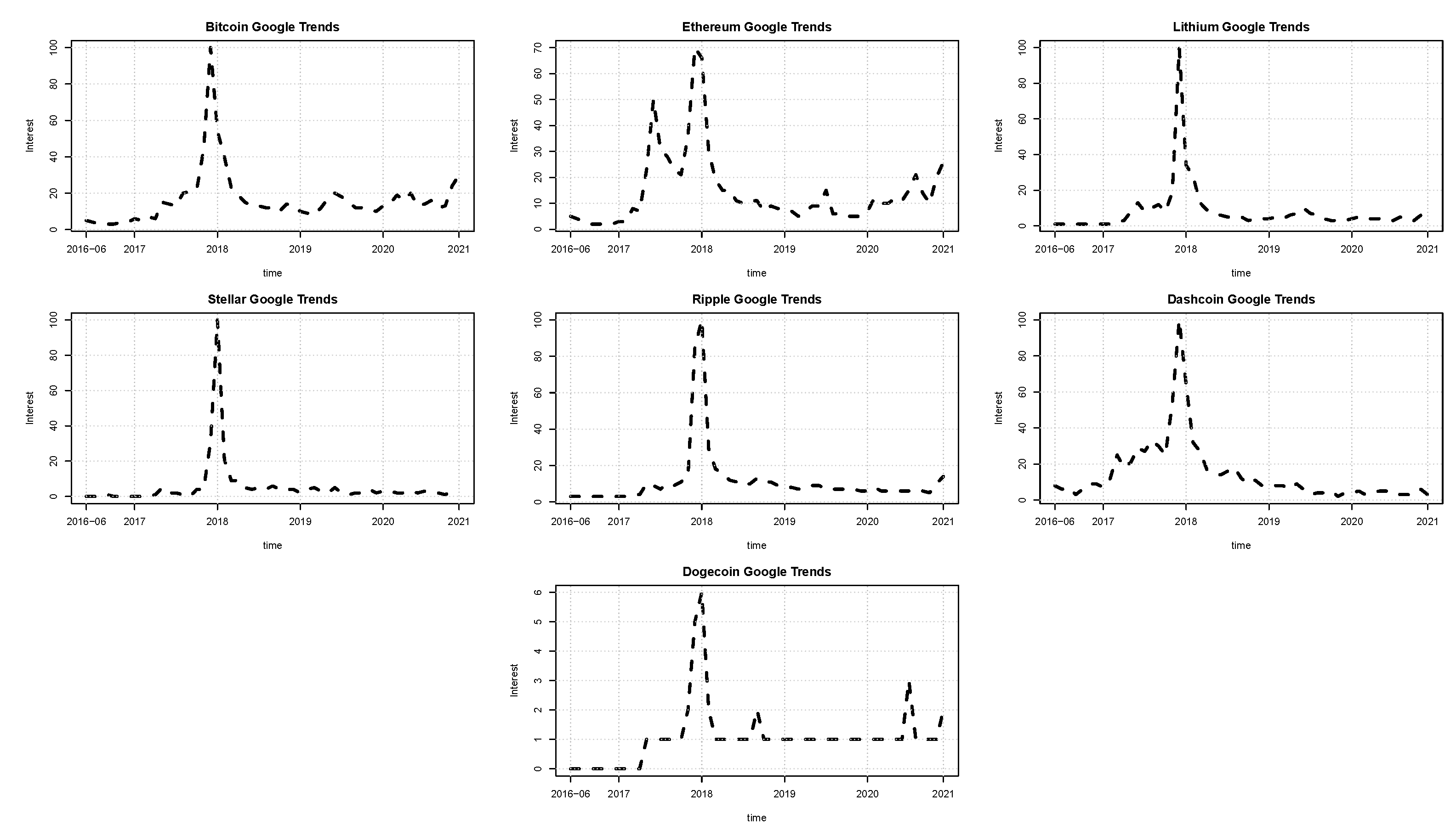
In this work, seven cryptocurrencies were used: Bitcoin, Ethereum, Lithium, Stellar, Ripple, Dashcoin, and Dogecoin. All the quotes for these series were collected from the Yahoo Finance site. The sample period is from June 2016 up to December 2020 for 1671 daily observations. The additional low-frequency volatility determinant is the Google trend series for each cryptocurrency. These Google trend series are reported monthly and enter Equation (12) as the first difference. The patterns of the cryptocurrencies and Google trend prices are illustrated in Figure 1 and Figure 2, respectively. In line with the literature, the connection between online searches and the prices’ movements appears evident. As of January 2018, all the online searches present a peak. Correspondingly, all the prices observed in January 2018 are at their maximum.
The main summary statistics for the close-to-close log-returns are reported in Table 2. All the returns exhibit a high kurtosis, sometimes a very high kurtosis, probably due to some exceptional values. Except for Bitcoin and Ethereum, all the returns are positively skewed. As also discussed in the Introduction, even though alternative approaches dealing with the fat tails and severe skewness are available in the literature, we use the Gaussian distribution for the estimation. Moreover, it has to be remarked that all the standard errors reported are based on Quasi-Maximum Likelihood methods, as was recently done by Guesmi et al. (2019), among others. Moreover, once is achieved, the resulting portfolio VaR will take care of the fat tails of the cryptocurrencies.
All the estimations performed in this work were executed in R using the package dccmidas (Candila 2021). The summary diagram in Figure 3 illustrates the phases of our research.
The results of the first step, concerning the univariate models, are reported in Table 3 and Table 4. The number of lagged realizations of the Google searches entering the long-run equation is . Interestingly, the parameters associated with the Google searches are almost always all significant. This means that such queries effectively help in estimating the volatility of digital currencies.
Once we obtained the standardized residuals, the second step of the estimation concerns the correlation models, whose estimated coefficients are reported in Table 5. The same table presents the averages of three robust (Laurent et al. 2013) loss functions—namely, the Euclidean, Squared Frobenius, and Root Mean Squared Error (RMSE). The losses evaluate the distance of the estimated1 conditional covariance matrix from the covariance proxy, which is represented by the matrix of the cross-products of . Finally, the SSM obtained from the MCS is highlighted in shades of gray. Surprisingly, under two out of three losses (i.e., the Euclidean and the Squared Frobenius), all the models using DAGM in the first step are in the SSM. When the RMSE is used, the DAGM-cDCC specification (that is, the model labeled as M4) is the only model belonging to the SSM. Therefore, it appears evident that including the (monthly) Google searches in the first step through a mixed-frequency approach results in better conditional covariance predictions. This observation is corroborated by the results of the test, which was applied to the standardized residuals obtained after the estimation of the conditional covariance matrix. Remarkably, the null hypothesis of no conditional heteroscedasticity was rejected for models M1, M2, and M3—that is, the parametric models without the Google trend information. Instead, both the parametric models using the MIDAS variable and the RM model do not reject the null hypothesis.
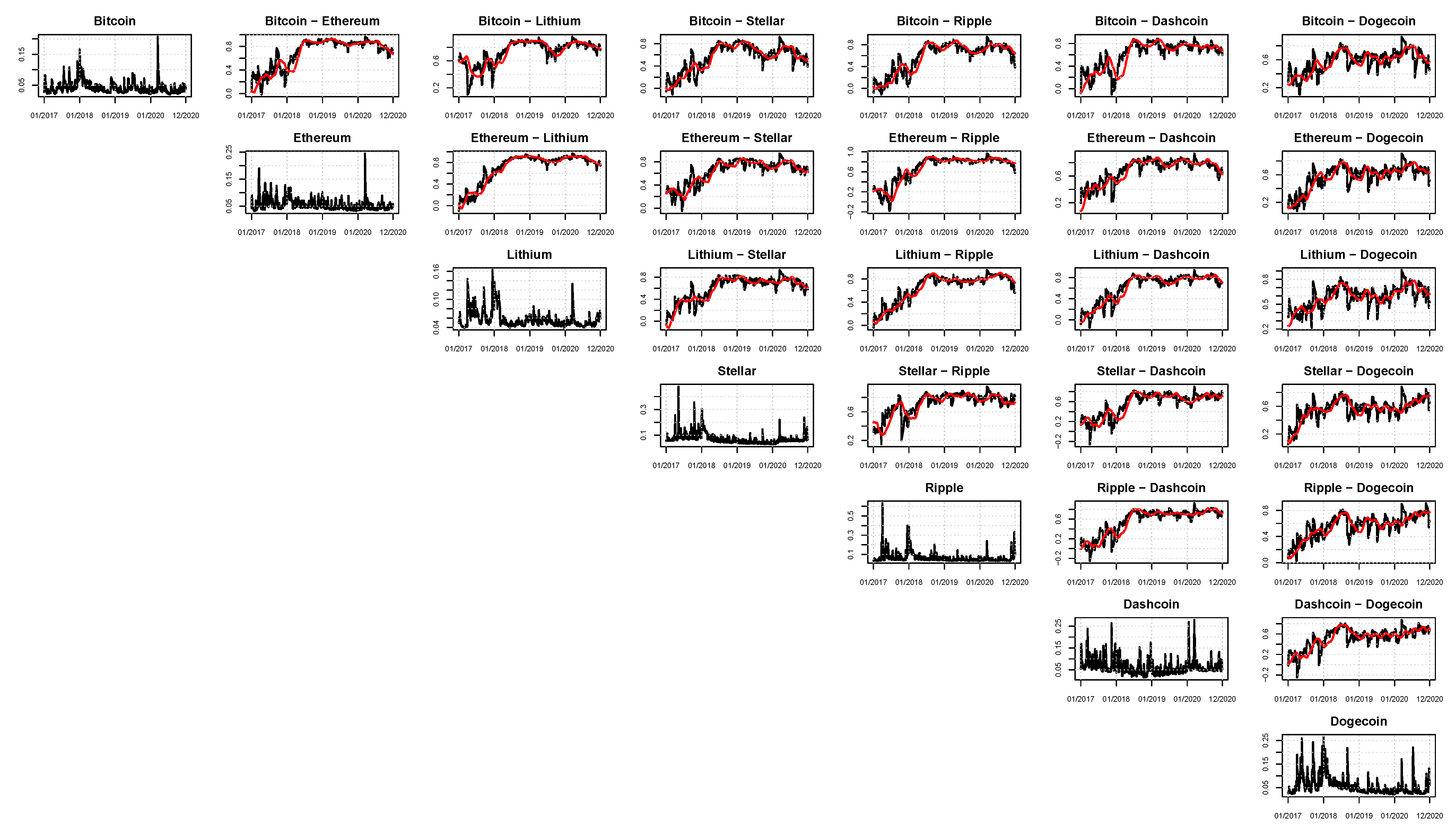
A graphical analysis of the correlation plots of the models belonging to the SSM (according to Euclidean and Squared Frobenius loss functions) is fundamental to visualize the time-varying patterns of the estimated correlations. Figure 4, Figure 5 and Figure 6 are dedicated to these plots, respectively, for models M4 (DAGM + cDCC), M5 (DAGM + DCC-MIDAS), and M6 (DAGM + DECO). Independently of the model adopted for the correlations, all the cryptocurrencies appear to be highly correlated. In particular, if the correlations seem low at the beginning of the considered sample, during the last period the digital currencies exhibit larger and generally very high interdependencies, almost always ranging between 0.6 and 0.8. From a portfolio manager’s perspective, these interconnections are fundamental to deciding the assets in which to invest.
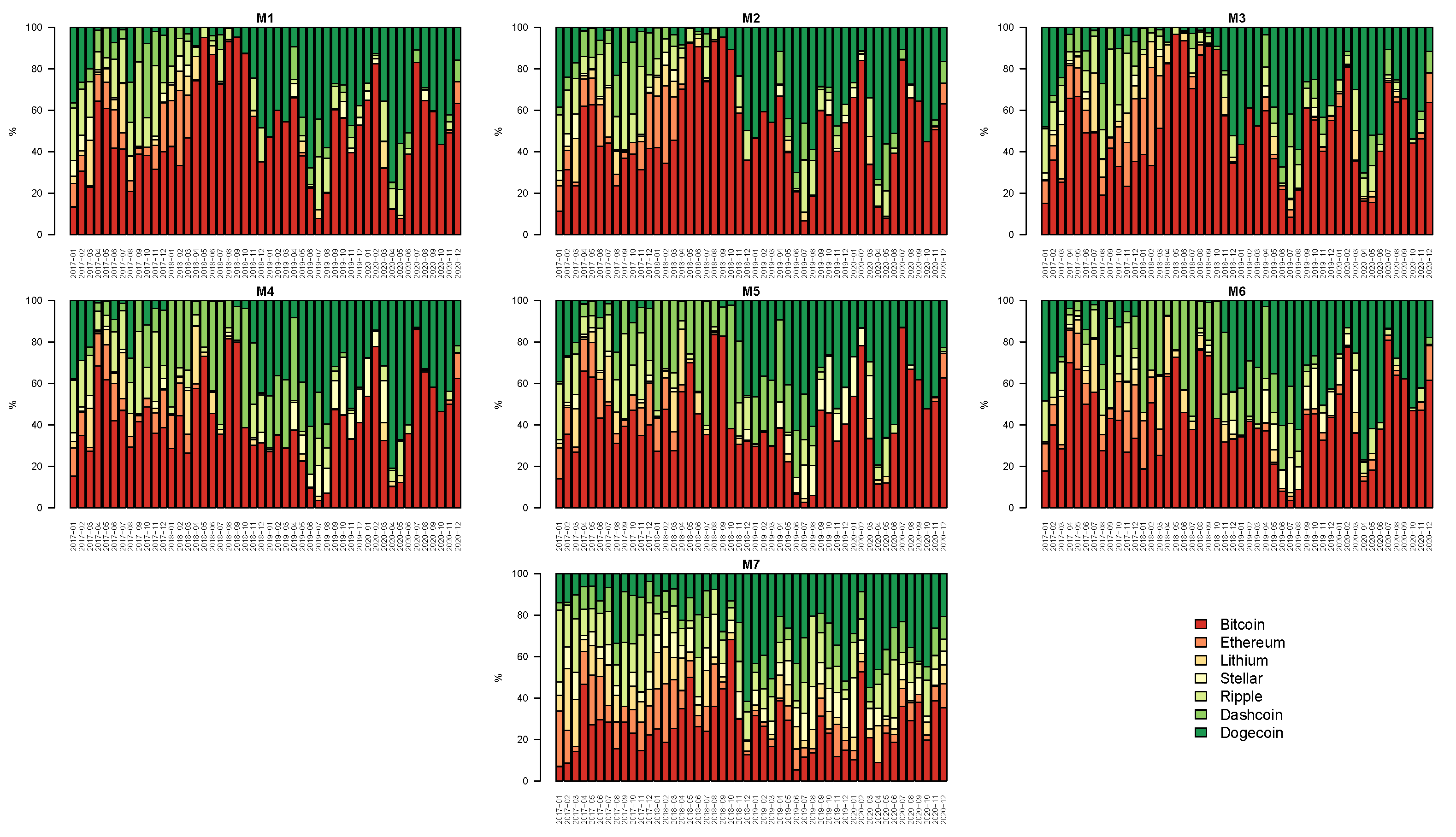
The last part of our analysis concerns the economic evaluation of the models. In particular, starting from each conditional covariance matrix , we calculated the optimal (daily) weights minimizing the portfolio variance (Markowitz 1952), as has also been done by Symitsi and Chalvatzis (2019), where the portfolio investigated consists of Bitcoin and other asset classes. Figure 7 summarizes the patterns of the estimated weights across time, cryptocurrencies, and models. Similar to Cipollini et al. (2021), each bar in the figure represents the rescaled summation of the daily weights by month. Overall, it can be noted that the GMV portfolio is mainly made up of Bitcoin for the parametric models. In other words, Bitcoin has the largest importance relative to the other digital currencies in the GMV portfolio. The optimal weights are then used for obtaining the portfolio return and variance. In particular, we calculated the VaR at level using the following parametric (Jorion 1997) approach:
where is the conditional mean of the portfolio, is the portfolio standard deviation, and is the inverse of Student’s t cumulative density function with degrees of freedom. Note that in Equation (15), we use a Student’s t distribution to explicitly take into account the fat tails of the cryptocurrencies. Finally, each VaR series coming from models M1 to M7 is evaluated through the MCS procedure using the following quantile loss (), as in González-Rivera et al. (2004):
where is the portfolio return and is an indicator function that is equal to one if the argument is true. The estimations of the degrees of freedom , as well as the results of the MCS tests, are reported in Table 6. The VaR series are calculated according to three different levels: 0.01, 0.05, and 0.10. The estimated degrees of freedom are very low, which is in agreement with the fat tails reported in Table 2. Interestingly, all the models belonging to the SSM as described by the statistical evaluation are again included in the SSM. To conclude, the inclusion of the Google trends in the univariate part of the DCC specifications dramatically improves the performance of the models from statistical and economic points of view.
4. Conclusions
The literature on financial econometrics has recently shown an enormous interest in cryptocurrencies. The first and most well-known digital currency, Bitcoin, dates back to 2009; today, thousands of cryptocurrencies are traded. From this aspect, cryptocurrencies can be used for speculative or hedging purposes. For this reason, investigating the volatility as well as the correlations of digital currencies appears to be extremely important. Although there are several contributions concerning the cryptocurrencies’ single variability and co-movements, the interdependencies of the daily cryptocurrencies potentially driven by additional variables, observed at lower frequencies, still remain unexplored. This paper aims to fill this gap. In particular, this work aims to estimate the conditional covariance matrix for a panel of cryptocurrencies using some specifications belonging to the Dynamic Conditional Correlation (DCC) class of models. The original contribution of this paper is the inclusion of the monthly Google queries regarding the cryptocurrencies as an additional volatility determinant in the DCC models’ univariate step. The inclusion of the monthly Google searches in models where the dependent variable is observed daily took place using the mixed-frequency proposed by Ghysels et al. (2007). In particular, for the first time, the Double Asymmetric GARCH–MIDAS (Amendola et al. 2019) was inserted within some DCC specifications. In doing so, the daily conditional covariance matrices also depended on the additional MIDAS variable—that is, the (first difference of the) Google trends. Once the time series of the conditional covariance matrices were obtained, statistical and economic evaluations of all the specifications employed were carried out. Both the evaluations were based on the selection of the set of superior models (SSM) according to the Model Confidence Set (MCS, Hansen et al. 2011) procedure. The statistical evaluation used robust (Laurent et al. 2013) loss functions. The economic evaluation was based on the estimation of the global minimum variance (GMV) portfolio, and then, on the analysis of the resulting Value-at-Risk (VaR). In terms of results, we found that the mixed-frequency approach provided good performances from both the statistical and economic perspectives. In particular, only the models employing the monthly Google searches belonged to the SSM. Instead, the excluded models were the DCC-based models using the simple GARCH specification for the univariate step and the RiskMetrics specification. The time-varying correlations of the models from the SSM showed that all the cryptocurrencies co-move together, mainly in the last part of the considered sample (June 2016–December 2020). In particular, the estimated correlations generally varied between 0.6 and 0.8, mainly in 2020. The economic analysis largely confirmed what was found in the statistical evaluation. In greater detail, the parametric approach was used to calculate the VaR of the GMV portfolio, with specific attention paid to the fat tails of the cryptocurrencies. Then, the VaR measures were evaluated through the MCS procedure according to the quantile loss (González-Rivera et al. 2004). Interestingly, again all the models based on a mixed-frequency approach entered the SSM. Last but not least, Bitcoin was the digital currency with the largest share in the considered GMV portfolio, independently of the specifications adopted.
Future research could enlarge the set of assets under investigation by including, for instance, standard currencies as well. Moreover, using different portfolio strategies could also be extremely useful. Furthermore, adopting some rolling forecasting schemes would be interesting. Finally, the multivariate models could also include specifications able to deal with the typical skewness and high kurtosis of the cryptocurrencies, such as the copula-based multivariate GARCH model of Lee and Long (2009) or the approach proposed by Paolella and Polak (2015) and then generalized in Paolella et al. (2019).
Funding
This research received no external funding.
Institutional Review Board Statement
Not applicable.
Informed Consent Statement
Not applicable.
Data Availability Statement
The cryptocurrencies used in this work are freely available from the Yahoo Finance site. Google trends data have been collected from the https://trends.google.com/ accessed on 30 June 2021, trends site.
Acknowledgments
The author would like to thank the editor-in-chief Marc S. Paolella, the guest editor Fredj Jawadi, and three anonymous referees for their very helpful and constructive comments.
Conflicts of Interest
The author declares no conflict of interest.
Abbreviations
The following abbreviations are used in this manuscript:
| DCC | Dynamic conditional correlation model (Engle 2002) |
| cDCC | Corrected DCC (Aielli 2013) |
| DECO | Dynamic equicorrelation (Engle and Kelly 2012) |
| RM | RiskMetrics |
| MIDAS | Mixing-Data Sampling |
| DAGM | Double Asymmetric GARCH–MIDAS model (Amendola et al. 2019) |
| M1 | GARCH for the univariate part and cDCC for the correlations |
| M2 | GARCH for the univariate part and DCC-MIDAS for the correlations |
| M3 | GARCH for the univariate part and DECO for the correlations |
| M4 | DAGM for the univariate part and cDCC for the correlations |
| M5 | DAGM for the univariate part and DCC-MIDAS for the correlations |
| M6 | DAGM for the univariate part and DECO for the correlations |
| M7 | RiskMetrics |
| SSM | Set of Superior Models |
| MCS | Model Confidence Set (Hansen et al. 2011) |
| GMV | Global Minimum Variance |
| 1 | In the case of the RiskMetrics model, the covariance matrix is calculated and not estimated. |
References
- Aielli, Gian Piero. 2013. Dynamic conditional correlation: On properties and estimation. Journal of Business & Economic Statistics 31: 282–99. [Google Scholar]
- Amendola, Alessandra, and Vincenzo Candila. 2017. Comparing multivariate volatility forecasts by direct and indirect approaches. Journal of Risk 19: 33–57. [Google Scholar] [CrossRef]
- Amendola, Alessandra, Vincenzo Candila, and Giampiero M. Gallo. 2019. On the asymmetric impact of macro–variables on volatility. Economic Modelling 76: 135–52. [Google Scholar] [CrossRef]
- Amendola, Alessandra, Manuela Braione, Vincenzo Candila, and Giuseppe Storti. 2020. A model confidence set approach to the combination of multivariate volatility forecasts. International Journal of Forecasting 36: 873–91. [Google Scholar] [CrossRef]
- Baek, Chung, and Matt Elbeck. 2015. Bitcoins as an investment or speculative vehicle? A first look. Applied Economics Letters 22: 30–34. [Google Scholar] [CrossRef]
- Bariviera, Aurelio F., María José Basgall, Waldo Hasperué, and Marcelo Naiouf. 2017. Some stylized facts of the Bitcoin market. Physica A: Statistical Mechanics and Its Applications 484: 82–90. [Google Scholar] [CrossRef] [Green Version]
- Bauwens, Luc, Sébastien Laurent, and Jeroen V. K. Rombouts. 2006. Multivariate GARCH models: A survey. Journal of Applied Econometrics 21: 79–109. [Google Scholar] [CrossRef] [Green Version]
- Bouri, Elie, Rangan Gupta, Aviral Kumar Tiwari, and David Roubaud. 2017. Does Bitcoin hedge global uncertainty? Evidence from wavelet-based quantile-in-quantile regressions. Finance Research Letters 23: 87–95. [Google Scholar] [CrossRef] [Green Version]
- Bouri, Elie, Syed Jawad Hussain Shahzad, David Roubaud, Ladislav Kristoufek, and Brian Lucey. 2020. Bitcoin, gold, and commodities as safe havens for stocks: New insight through wavelet analysis. The Quarterly Review of Economics and Finance 77: 156–64. [Google Scholar] [CrossRef]
- Candila, Vincenzo. 2021. Dccmidas: A Package for Estimating DCC-Based Models in R. R Package Version 0.1.0. Available online: https://www.researchgate.net/publication/350064227_dccmidas_A_package_for_estimating_DCC-based_models_in_R (accessed on 30 June 2021).
- Canh, Nguyen Phuc, Udomsak Wongchoti, Su Dinh Thanh, and Nguyen Trung Thong. 2019. Systematic risk in cryptocurrency market: Evidence from DCC-MGARCH model. Finance Research Letters 29: 90–100. [Google Scholar] [CrossRef]
- Caporale, Guglielmo Maria, and Timur Zekokh. 2019. Modelling volatility of cryptocurrencies using markov-switching GARCH models. Research in International Business and Finance 48: 143–55. [Google Scholar] [CrossRef]
- Catania, Leopoldo, Stefano Grassi, and Francesco Ravazzolo. 2018. Predicting the volatility of cryptocurrency time-series. In Mathematical and Statistical Methods for Actuarial Sciences and Finance. Edited by Marco Corazza, María Durbán, Aurea Grané, Cira Perna and Marilena Sibillo. Berlin: Springer, pp. 203–7. [Google Scholar]
- Cebrián-Hernández, Ángeles, and Enrique Jiménez-Rodríguez. 2021. Modeling of the Bitcoin Volatility through Key Financial Environment Variables: An Application of Conditional Correlation MGARCH Models. Mathematics 9: 267. [Google Scholar] [CrossRef]
- Chu, Jeffrey, Stephen Chan, Saralees Nadarajah, and Joerg Osterrieder. 2017. GARCH modelling of cryptocurrencies. Journal of Risk and Financial Management 10: 17. [Google Scholar] [CrossRef]
- Cipollini, Fabrizio, Giampiero M. Gallo, and Alessandro Palandri. 2021. A dynamic conditional approach to forecasting portfolio weights. International Journal of Forecasting 37: 1111–26. [Google Scholar] [CrossRef]
- Colacito, Riccardo, Robert F. Engle, and Eric Ghysels. 2011. A component model for dynamic correlations. Journal of Econometrics 164: 45–59. [Google Scholar] [CrossRef] [Green Version]
- Conrad, Christian, and Karin Loch. 2015. Anticipating long-term stock market volatility. Journal of Applied Econometrics 30: 1090–114. [Google Scholar] [CrossRef] [Green Version]
- Conrad, Christian, Anessa Custovic, and Eric Ghysels. 2018. Long- and short-term cryptocurrency volatility components: A GARCH-MIDAS analysis. Journal of Risk and Financial Management 11: 23. [Google Scholar] [CrossRef]
- ElBahrawy, Abeer, Laura Alessandretti, Anne Kandler, Romualdo Pastor-Satorras, and Andrea Baronchelli. 2017. Evolutionary dynamics of the cryptocurrency market. Royal Society Open Science 4: 1–9. [Google Scholar] [CrossRef] [Green Version]
- Elendner, Hermann, Simon Trimborn, Bobby Ong, and Teik Ming Lee. 2018. Chapter 7—The Cross-Section of Crypto-Currencies as Financial Assets: Investing in Crypto-Currencies Beyond Bitcoin. In Handbook of Blockchain, Digital Finance, and Inclusion, Volume 1. Edited by David Lee Kuo Chuen and Robert Deng. Cambridge: Academic Press, pp. 145–73. [Google Scholar]
- Engle, Robert F. 1982. Autoregressive conditional heteroscedasticity with estimates of the variance of United Kingdom inflation. Econometrica 50: 987–1007. [Google Scholar] [CrossRef]
- Engle, Robert F. 2002. Dynamic conditional correlation: A simple class of multivariate generalized autoregressive conditional heteroskedasticity models. Journal of Business & Economic Statistics 20: 339–50. [Google Scholar]
- Engle, Robert F., and Bryan Kelly. 2012. Dynamic equicorrelation. Journal of Business & Economic Statistics 30: 212–28. [Google Scholar]
- Engle, Robert F., and Kennett F. Kroner. 1995. Multivariate simultaneous generalized ARCH. Econometric Theory 11: 122–50. [Google Scholar] [CrossRef]
- Engle, Robert F., Eric Ghysels, and Bumjean Sohn. 2013. Stock market volatility and macroeconomic fundamentals. Review of Economics and Statistics 95: 776–97. [Google Scholar] [CrossRef]
- Gandal, Neil, and Hanna Halaburda. 2016. Can we predict the winner in a market with network effects? Competition in cryptocurrency market. Games 7: 16. [Google Scholar] [CrossRef] [Green Version]
- García-Medina, Andrés, and José B. Hernández Chaudary. 2020. Network analysis of multivariate transfer entropy of cryptocurrencies in times of turbulence. Entropy 22: 760. [Google Scholar] [CrossRef]
- Ghysels, Eric, Arthur Sinko, and Rossen Valkanov. 2007. MIDAS regressions: Further results and new directions. Econometric Reviews 26: 53–90. [Google Scholar] [CrossRef]
- González-Rivera, Gloria, Tae-Hwy Lee, and Santosh Mishra. 2004. Forecasting volatility: A reality check based on option pricing, utility function, value-at-risk, and predictive likelihood. International Journal of Forecasting 20: 629–45. [Google Scholar] [CrossRef]
- Guesmi, Khaled, Samir Saadi, Ilyes Abid, and Zied Ftiti. 2019. Portfolio diversification with virtual currency: Evidence from bitcoin. International Review of Financial Analysis 63: 431–37. [Google Scholar] [CrossRef]
- Hansen, Peter R., Asger Lunde, and James M. Nason. 2011. The Model Confidence Set. Econometrica 79: 453–97. [Google Scholar] [CrossRef] [Green Version]
- Hemche, Omar, Fredj Jawadi, Samir B Maliki, and Abdoulkarim Idi Cheffou. 2016. On the study of contagion in the context of the subprime crisis: A dynamic conditional correlation–multivariate GARCH approach. Economic Modelling 52: 292–99. [Google Scholar] [CrossRef]
- Hileman, Garrick, and Michel Rauchs. 2017. Global cryptocurrency benchmarking study. Cambridge Centre for Alternative Finance 33: 33–113. [Google Scholar]
- Ji, Qiang, Elie Bouri, Chi Keung Marco Lau, and David Roubaud. 2019. Dynamic connectedness and integration in cryptocurrency markets. International Review of Financial Analysis 63: 257–72. [Google Scholar] [CrossRef]
- Jorion, Philippe. 1997. Value at Risk. Chicago: Irwin. [Google Scholar]
- Katsiampa, Paraskevi, Shaen Corbet, and Brian Lucey. 2019. High frequency volatility co-movements in cryptocurrency markets. Journal of International Financial Markets, Institutions and Money 62: 35–52. [Google Scholar] [CrossRef]
- Kristoufek, Ladislav. 2013. BitCoin meets Google Trends and Wikipedia: Quantifying the relationship between phenomena of the Internet era. Scientific Reports 3: 1–7. [Google Scholar] [CrossRef] [Green Version]
- Kumar, Anoop S., and Suvvari Anandarao. 2019. Volatility spillover in crypto-currency markets: Some evidences from GARCH and wavelet analysis. Physica A: Statistical Mechanics and Its Applications 524: 448–58. [Google Scholar] [CrossRef]
- Laurent, Sébastien, Jeroen V. K. Rombouts, and Francesco Violante. 2013. On loss functions and ranking forecasting performances of multivariate volatility models. Journal of Econometrics 173: 1–10. [Google Scholar] [CrossRef] [Green Version]
- Lee, Tae-Hwy, and Xiangdong Long. 2009. Copula-based multivariate GARCH model with uncorrelated dependent errors. Journal of Econometrics 150: 207–18. [Google Scholar] [CrossRef] [Green Version]
- Ling, Shiqing, and Wai-Keung Li. 1997. Diagnostic checking of nonlinear multivariate time series with multivariate ARCH errors. Journal of Time Series Analysis 18: 447–64. [Google Scholar] [CrossRef]
- Markowitz, Harry. 1952. Portfolio selection. The Journal of Finance 7: 77–91. [Google Scholar]
- Mensi, Walid, Khamis Hamed Al-Yahyaee, Idries Mohammad Wanas Al-Jarrah, Xuan Vinh Vo, and Sang Hoon Kang. 2020. Dynamic volatility transmission and portfolio management across major cryptocurrencies: Evidence from hourly data. The North American Journal of Economics and Finance 54: 1–14. [Google Scholar] [CrossRef]
- Näf, Jeffrey, Marc S. Paolella, and Paweł Polak. 2019. Heterogeneous tail generalized COMFORT modeling via Cholesky decomposition. Journal of Multivariate Analysis 172: 84–106. [Google Scholar] [CrossRef]
- Nakamoto, Satoshi. 2008. Bitcoin: A Peer-to-Peer Electronic Cash System. Technical Report, Manubot. Available online: https://bitcoin.org/en/bitcoin-paper (accessed on 30 June 2021).
- Paolella, Marc S., and Paweł Polak. 2015. COMFORT: A common market factor non-Gaussian returns model. Journal of Econometrics 187: 593–605. [Google Scholar] [CrossRef] [Green Version]
- Paolella, Marc S., Paweł Polak, and Patrick S. Walker. 2019. Regime switching dynamic correlations for asymmetric and fat-tailed conditional returns. Journal of Econometrics 213: 493–515. [Google Scholar] [CrossRef]
- Pesaran, Bahram, and M. Hashem Pesaran. 2010. Conditional volatility and correlations of weekly returns and the VaR analysis of 2008 stock market crash. Economic Modelling 27: 1398–416. [Google Scholar] [CrossRef] [Green Version]
- Shi, Yongjing, Aviral Kumar Tiwari, Giray Gozgor, and Zhou Lu. 2020. Correlations among cryptocurrencies: Evidence from multivariate factor stochastic volatility model. Research in International Business and Finance 53: 1–11. [Google Scholar] [CrossRef]
- Symitsi, Efthymia, and Konstantinos J. Chalvatzis. 2019. The economic value of Bitcoin: A portfolio analysis of currencies, gold, oil and stocks. Research in International Business and Finance 48: 97–110. [Google Scholar] [CrossRef] [Green Version]
- Teräsvirta, Timo. 2009. An introduction to univariate GARCH models. In Handbook of Financial Time Series. Berlin: Springer, pp. 17–42. [Google Scholar]
- Walther, Thomas, Tony Klein, and Elie Bouri. 2019. Exogenous drivers of bitcoin and cryptocurrency volatility—A mixed data sampling approach to forecasting. Journal of International Financial Markets, Institutions and Money 63: 101–33. [Google Scholar] [CrossRef]
- Weber, Beat. 2016. Bitcoin and the legitimacy crisis of money. Cambridge Journal of Economics 40: 17–41. [Google Scholar] [CrossRef]
- Yermack, David. 2015. Is Bitcoin a real currency? An economic appraisal. In Handbook of Digital Currency. Edited by David Lee Kuo Chuen. Cambridge: Academic Press, pp. 31–43. [Google Scholar]
- Zhang, Wei, Pengfei Wang, Xiao Li, and Dehua Shen. 2018. Some stylized facts of the cryptocurrency market. Applied Economics 50: 5950–65. [Google Scholar] [CrossRef]
Figure 1.
Plots of prices. Sample period: June 2016 to December 2020. Number of observations: 1671.

Figure 2.
Plots of Google trends. Sample period: June 2016 to December 2020. Number of monthly observations: 55.
Figure 2.
Plots of Google trends. Sample period: June 2016 to December 2020. Number of monthly observations: 55.

Figure 3.
Summary diagram.

Figure 4.
Plots of volatilities (main diagonal) and correlations for the model M4: DAGM for the univariate part and cDCC for the correlations. Sample period: January 2017 to December 2020. Number of daily observations: 1457.
Figure 4.
Plots of volatilities (main diagonal) and correlations for the model M4: DAGM for the univariate part and cDCC for the correlations. Sample period: January 2017 to December 2020. Number of daily observations: 1457.

Figure 5.
Plots of volatilities (main diagonal) and correlations for the model M5: DAGM for the univariate part and DCC-MIDAS for the correlations. Red lines represent the long-run correlation. Sample period: January 2017 to December 2020. Number of daily observations: 1457.
Figure 5.
Plots of volatilities (main diagonal) and correlations for the model M5: DAGM for the univariate part and DCC-MIDAS for the correlations. Red lines represent the long-run correlation. Sample period: January 2017 to December 2020. Number of daily observations: 1457.

Figure 6.
Plots of volatilities (main diagonal) and correlations for the model M6: DAGM for the univariate part and DECO for the correlations. Sample period: January 2017 to December 2020. Number of daily observations: 1457.
Figure 6.
Plots of volatilities (main diagonal) and correlations for the model M6: DAGM for the univariate part and DECO for the correlations. Sample period: January 2017 to December 2020. Number of daily observations: 1457.

Figure 7.
Plots of weights’ importance by month, according to the GMV portfolio.


Table 1.
Functional forms of the covariance models.
| Model | Functional Form |
|---|---|
| cDCC (Aielli 2013) | |
| DCC-MIDAS (Colacito et al. 2011) | |
| DECO (Engle and Kelly 2012) | |
| RiskMetrics | |
Notes: The table reports the multivariate model dynamics of the different specifications employed in the empirical section. represents the long-run correlation as in Equation (2.12) of Colacito et al. (2011). denotes the identity matrix, a matrix of ones, and a vector of ones.
Table 2.
Summary statistics.
| Min. | Max. | Mean | SD | Skew. | Kurt. | |
|---|---|---|---|---|---|---|
| Bitcoin | −0.465 | 0.225 | 0.002 | 0.041 | −0.911 | 13.535 |
| Ethereum | −0.551 | 0.290 | 0.002 | 0.056 | −0.538 | 9.586 |
| Lithium | −0.449 | 0.511 | 0.002 | 0.058 | 0.717 | 11.599 |
| Stellar | −0.410 | 0.723 | 0.003 | 0.077 | 1.968 | 17.156 |
| Ripple | −0.616 | 1.027 | 0.002 | 0.071 | 2.407 | 39.494 |
| Dashcoin | −0.459 | 0.438 | 0.001 | 0.058 | 0.605 | 9.009 |
| Dogecoin | −0.493 | 0.477 | 0.002 | 0.062 | 0.792 | 12.843 |
Notes: The table presents the main statistics (the minimum (Min.) and maximum (Max.), the mean, standard deviation (SD), skewness (Skew.) and excess kurtosis (Kurt.)) for the close-to-close log-returns. Sample period: June 2016–December 2020. Number of observations: 1671.
Table 3.
M1, M2 and M3: univariate models.
| Estimate | Std. Error | t Value | Pr(>|t|) | Sig. | |
|---|---|---|---|---|---|
| Bitcoin | |||||
| 0.000 | 0.000 | 2.856 | 0.004 | *** | |
| 0.181 | 0.053 | 3.393 | 0.001 | *** | |
| 0.790 | 0.029 | 27.214 | 0.000 | *** | |
| Ethereum | |||||
| 0.000 | 0.000 | 2.892 | 0.004 | *** | |
| 0.182 | 0.044 | 4.103 | 0.000 | *** | |
| 0.733 | 0.059 | 12.424 | 0.000 | *** | |
| Lithium | |||||
| 0.000 | 0.000 | 1.493 | 0.135 | ||
| 0.071 | 0.028 | 2.562 | 0.010 | ** | |
| 0.878 | 0.046 | 19.096 | 0.000 | *** | |
| Stellar | |||||
| 0.000 | 0.000 | 1.744 | 0.081 | * | |
| 0.219 | 0.070 | 3.135 | 0.002 | *** | |
| 0.752 | 0.079 | 9.534 | 0.000 | *** | |
| Ripple | |||||
| 0.000 | 0.000 | 2.281 | 0.023 | ** | |
| 0.374 | 0.152 | 2.455 | 0.014 | ** | |
| 0.609 | 0.117 | 5.225 | 0.000 | *** | |
| Dashcoin | |||||
| 0.000 | 0.000 | 2.663 | 0.008 | *** | |
| 0.236 | 0.070 | 3.394 | 0.001 | *** | |
| 0.744 | 0.062 | 11.990 | 0.000 | *** | |
| Dogecoin | |||||
| 0.000 | 0.000 | 2.585 | 0.010 | *** | |
| 0.230 | 0.044 | 5.276 | 0.000 | *** | |
| 0.769 | 0.039 | 19.623 | 0.000 | *** | |
Notes: The table reports the estimates of the univariate GARCH models used in the M2, M3 and M4 specifications. Column Std. Error reports the Quasi-Maximum Likelihood standard errors. Sample Period: June 2016 to December 2020. Number of daily observations: 1671. *, ** and *** represent the significance at levels , respectively.
Table 4.
M4, M5 and M6: univariate models.
| Estimate | Std. Error | t Value | Pr(>|t|) | Sig. | |
|---|---|---|---|---|---|
| Bitcoin | |||||
| 0.192 | 0.048 | 4.037 | 0.000 | *** | |
| 0.765 | 0.027 | 27.837 | 0.000 | *** | |
| m | −6.381 | 0.977 | −6.532 | 0.000 | *** |
| 0.364 | 0.169 | 2.156 | 0.031 | ** | |
| 1.739 | 0.720 | 2.415 | 0.016 | ** | |
| 0.183 | 0.129 | 1.421 | 0.155 | ||
| 2.698 | 0.976 | 2.763 | 0.006 | *** | |
| Ethereum | |||||
| 0.189 | 0.041 | 4.548 | 0.000 | *** | |
| 0.698 | 0.066 | 10.622 | 0.000 | *** | |
| m | −6.029 | 0.314 | −19.201 | 0.000 | *** |
| 0.218 | 0.080 | 2.729 | 0.006 | *** | |
| 2.323 | 0.638 | 3.639 | 0.000 | *** | |
| 0.071 | 0.049 | 1.434 | 0.152 | ||
| 8.893 | 4.558 | 1.951 | 0.051 | * | |
| Lithium | |||||
| 0.072 | 0.034 | 2.156 | 0.031 | ** | |
| 0.849 | 0.073 | 11.560 | 0.000 | *** | |
| m | −5.876 | 0.294 | −19.970 | 0.000 | *** |
| 0.043 | 0.022 | 1.944 | 0.052 | * | |
| 2.148 | 1.036 | 2.074 | 0.038 | ** | |
| 0.033 | 0.027 | 1.194 | 0.233 | ||
| 3.764 | 4.435 | 0.849 | 0.396 | ||
| Stellar | |||||
| 0.274 | 0.091 | 2.991 | 0.003 | *** | |
| 0.501 | 0.156 | 3.217 | 0.001 | *** | |
| m | −5.000 | 0.275 | −18.181 | 0.000 | *** |
| 0.059 | 0.020 | 2.988 | 0.003 | *** | |
| 1.758 | 0.334 | 5.263 | 0.000 | *** | |
| 0.092 | 0.020 | 4.677 | 0.000 | *** | |
| 1.209 | 0.158 | 7.676 | 0.000 | *** | |
| Ripple | |||||
| 0.346 | 0.114 | 3.031 | 0.002 | *** | |
| 0.569 | 0.110 | 5.174 | 0.000 | *** | |
| m | −5.313 | 0.629 | −8.447 | 0.000 | *** |
| 0.036 | 0.014 | 2.628 | 0.009 | *** | |
| 4.307 | 1.350 | 3.190 | 0.001 | *** | |
| 0.013 | 0.006 | 2.218 | 0.027 | ** | |
| 8.188 | 1.714 | 4.777 | 0.000 | *** | |
| Dashcoin | |||||
| 0.347 | 0.114 | 3.039 | 0.002 | *** | |
| 0.652 | 0.114 | 5.696 | 0.000 | *** | |
| m | −0.074 | 0.309 | −0.238 | 0.812 | |
| −0.046 | 0.049 | −0.957 | 0.339 | ||
| 1.992 | 0.908 | 2.193 | 0.028 | ** | |
| 0.077 | 0.041 | 1.895 | 0.058 | * | |
| 1.986 | 0.827 | 2.402 | 0.016 | ** | |
| Dogecoin | |||||
| 0.226 | 0.042 | 5.374 | 0.000 | *** | |
| 0.743 | 0.052 | 14.204 | 0.000 | *** | |
| m | −5.615 | 0.613 | −9.167 | 0.000 | *** |
| 0.060 | 0.022 | 2.663 | 0.008 | *** | |
| 2.064 | 0.570 | 3.618 | 0.000 | *** | |
| 0.021 | 0.025 | 0.827 | 0.408 | ||
| 1.465 | 0.761 | 1.925 | 0.054 | * | |
Notes: The table reports the estimates of the univariate DAGM models used in the M4, M5 and M6 specifications. Column Std. Error reports the Quasi-Maximum Likelihood based standard errors. The MIDAS variables are represented by the first difference of the Google trends. Sample Period: June 2016 to December 2020. Number of daily observations: 1671. *, ** and *** represent the significance at levels , respectively.
Table 5.
Correlation estimates, MCS and residual diagnostics.
| M1 | M2 | M3 | M4 | M5 | M6 | M7 | |
|---|---|---|---|---|---|---|---|
| a | 0.017 ** | 0.038 | 0.086 ** | 0.018 *** | 0.034 | 0.089 *** | |
| (0.008) | (0.031) | (0.044) | (0.006) | (0.161) | (0.022) | ||
| b | 0.982 *** | 0.931 *** | 0.913 *** | 0.981 *** | 0.937 * | 0.91 *** | |
| (0.008) | (0.089) | (0.054) | (0.007) | (0.483) | (0.019) | ||
| 1.001 | 1.001 | ||||||
| (1.793) | (11.109) | ||||||
| Euclidean | 4.496 | 4.503 | 4.515 | 4.413 | 4.419 | 4.447 | 6.683 |
| Sq. Frobenius | 2.630 | 2.630 | 2.630 | 2.556 | 2.556 | 2.556 | 3.650 |
| RMSE | 1.526 | 1.531 | 1.528 | 1.515 | 1.522 | 1.519 | 1.563 |
| 11.941 *** | 14.631 *** | 8.657 *** | 5.659 | 6.281 | 5.448 | 0.004 | |
| 12.487 *** | 15.525 *** | 8.744 ** | 5.756 | 6.521 | 5.525 | 0.004 |
Notes: Top panel reports the estimates for the correlation models. Numbers in parentheses are the Quasi-Maximum Likelihood standard errors. Bottom panel reports the average losses, according to the three loss functions in the first column. Sq. Frobenius stands for Squared Frobenius and RMSE for Root Mean Squared Error. The reported averages for the Euclidean, Squared Frobenius, and RMSE have been multiplied by 1000, 1000, and 10, respectively. Shades of gray denote inclusion in the SSM at significance level . and report the test statistics, whose null is of no conditional heteroscedasticity. *, ** and *** represent the significance at levels , respectively. Estimation period: June 2016 to December 2020, number of daily observations: 1671. Evaluation period: January 2017 to December 2020, number of daily observations: 1457.
Table 6.
Portfolio evaluation.
| M1 | M2 | M3 | M4 | M5 | M6 | M7 | |
|---|---|---|---|---|---|---|---|
| 2.224 | 2.249 | 2.204 | 2.369 | 2.380 | 2.368 | 2.199 | |
| 0.208 | 0.2 | 0.209 | 0.185 | 0.183 | 0.184 | 0.904 | |
| 0.576 | 0.562 | 0.584 | 0.542 | 0.537 | 0.542 | 1.201 | |
| 0.803 | 0.788 | 0.813 | 0.781 | 0.776 | 0.783 | 1.323 |
Notes: Top panel reports the estimates for the degrees of freedom ν of the Student’s t distribution, used to calculate the VaR series. Bottom panel reports the average QL losses, according to the three τ levels in the first column. Shades of gray denote inclusion in the SSM at significance level α = 0.10. Estimation period: June 2016 to December 2020, number of daily observations: 1671. Evaluation period: January 2017 to December 2020, number of daily observations: 1457.
Publisher’s Note: MDPI stays neutral with regard to jurisdictional claims in published maps and institutional affiliations. |
© 2021 by the author. Licensee MDPI, Basel, Switzerland. This article is an open access article distributed under the terms and conditions of the Creative Commons Attribution (CC BY) license (https://creativecommons.org/licenses/by/4.0/).
Share and Cite
MDPI and ACS Style
Candila, V. Multivariate Analysis of Cryptocurrencies. Econometrics 2021, 9, 28. https://doi.org/10.3390/econometrics9030028
AMA Style
Candila V. Multivariate Analysis of Cryptocurrencies. Econometrics. 2021; 9(3):28. https://doi.org/10.3390/econometrics9030028
Chicago/Turabian StyleCandila, Vincenzo. 2021. "Multivariate Analysis of Cryptocurrencies" Econometrics 9, no. 3: 28. https://doi.org/10.3390/econometrics9030028
Note that from the first issue of 2016, this journal uses article numbers instead of page numbers. See further details here.