Surface Mass-Balance Gradients From Elevation and Ice Flux Data in the Columbia Basin, Canada

1 Introduction

Variation of surface mass balance with elevation, also known as a mass-balance gradient, characterizes the relation between a given glacier and climate (Meier and Post, 1962; Oerlemans and Hoogendoorn, 1989; Vallon et al., 1998), and regionally determines glacier distribution (Furbish and Andrews, 1984). Regional glacier models (e.g., Radić and Hock, 2011; Clarke et al., 2015; Rounce et al., 2020) must accurately represent balance gradients to reliably estimate ice flux. The distribution of mass balance is typically either prescribed using available glaciological balance data (Farinotti et al., 2009; Huss and Farinotti, 2012; Clarke et al., 2013; Bach et al., 2018) or simulated and calibrated with available mass-balance data (Clarke et al., 2015; Maussion et al., 2019). Observations of balance gradients are uncommon (Rea, 2009; WGMS, 2018) which hampers accurate model simulation of balance gradients. Geodetic estimates of mass change have become widespread (e.g., Berthier et al., 2014; Brun et al., 2017), but these estimates cannot be used to infer mass balance with elevation since elevation change at-a-point arises from both surface mass change and ice flux. Methods to quantify ice flux exist (e.g., Gudmundsson and Bauder, 1999; Berthier et al., 2003; Jarosch, 2008; Vincent et al., 2009; Bisset et al., 2020) but are limited in application by lack of input data regarding elevation and ice-flux changes.

The continuity equation shows the relationship between the rate of change of glacier thickness ($\dot{h}$), the glacier mass-balance ($\dot{b}$), and the flux divergence ($\nabla \cdot \overrightarrow{q}$) (Cogley et al., 2011):

We assume that $\dot{h}$ is equal to the rate of elevation change, and $\dot{b}$ is equal to the surface mass-balance rate as we assume that the basal and internal mass-balance components are negligible. The continuity equation (Eq. 1), applied to glaciers, indicates that the two primary processes that drive recent thinning are a warmer climate favoring ablation (O’Neel et al., 2019), and decreasing ice flux from upstream regions (Heid and Kääb, 2012; Dehecq et al., 2019). Ice flux is directly influenced by changes in local mass balance which affects glacier thickness and thereby the driving stress and local deformation at a given point.

Publically-available data now exist to estimate mass balance from the continuity equation (Eq. 1): surface height change data for glaciers (e.g., Berthier et al., 2014; Brun et al., 2017); density and glacier facies (Rabatel et al., 2017; Pelto et al., 2019); ice velocity (e.g., Burgess et al., 2013; Dehecq et al., 2019; Gardner et al., 2020); and ice thickness (e.g., Farinotti et al., 2019). Fewer than 1% of glaciers worldwide have long-term mass-balance observations (WGMS, 2018) or observations of subglacial topography (GlaThiDa, 2019). The lack of subglacial topographic information limits calculation of ice flux to relatively few glaciers (e.g., Berthier et al., 2003; Vincent et al., 2009; Belart et al., 2017; Rabatel et al., 2018; Bisset et al., 2020; Young et al., 2020). Previous efforts to infer the spatial distribution of mass balance from ice flux have primarily focused on glacier tongues (e.g., Gudmundsson and Bauder, 1999; Kääb and Funk, 1999; Berthier et al., 2003; Vincent et al., 2009, 2021; Berthier and Vincent, 2012; Gao et al., 2020), where ice thickness, glaciological balance and ice velocity measurements are most numerous, density is assumed to be that of ice, and glacier geometry is simplest.

The primary motivation for our study is to examine whether we can use remotely-sensed data to reliably estimate the altitude-mass balance relation (balance gradients) for five glaciers in the Columbia Basin, Canada. We use sequential airborne laser scanning (ALS) digital elevation models (DEMs) to calculate elevation-dependent changes in surface elevation and ice flow. We combine these data with radar surveys (Pelto et al., 2020) and ice thickness maps produced from surface inversion (Farinotti et al., 2019; Pelto et al., 2020) to solve the continuity equation (Eq. 1) using a “flux gate approach” (Berthier and Vincent, 2012). Flux gates provide the relation of mass balance to altitude by inferring the average surface mass balance between (or above or below) selected cross sections where the bedrock topography is known. This approach does not yield a complete spatial coverage of glacier mass balance, but is simpler and less data demanding than alternative methods (e.g., Hubbard et al., 2000; Sold et al., 2013; Belart et al., 2017; Young et al., 2020), and thus easier to apply for more glaciers. We collected field observations of surface mass balance ($b_a$) coincident with the ALS surveys (Pelto et al., 2019), and use these data to assess the accuracy of our flux-derived $b_a$. Given that observations of ice thickness are a limiting factor for all methods to infer the distribution of $b_a$ from ice flux, we also test whether model estimates of ice thickness produce reasonable ice flux and $b_a$ estimates relative to observed ice thickness.

2 Study Area: Columbia Mountains, Canada

The Columbia Mountains are located in southeastern British Columbia, Canada and contain over 2,300 glaciers covering 1960 km² (Bolch et al., 2010). These glaciers provide runoff to the Columbia and Fraser rivers (Figure 1). We selected five glaciers for which glaciological mass-balance measurements, geodetic surveys and ice thickness data exist: Conrad, Illecillewaet, Kokanee, Nordic, and Zillmer glaciers (Figure 1). Conrad Glacier is a valley glacier in the Purcell Mountains bordering Bugaboo Provincial Park with a 1,400 m elevation range (Table 1). Comprising half of Illecillewaet Névé, the broad Illecillewaet Glacier is part of a 22 km² icefield within the Selkirk Mountains in Glacier National Park. Kokanee Glacier is a broad, small (1.8 km²) alpine glacier in the Purcell Mountains. Nordic Glacier is a steep alpine glacier in the Selkirk Mountains on the northern boundary of Glacier National Park. Zillmer Glacier is located in the Premier Range at the far north-western edge of the Columbia Basin.

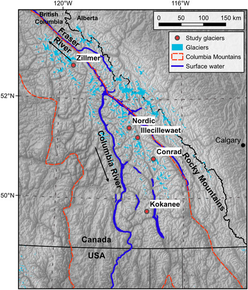
FIGURE 1. Study glaciers of the Columbia Mountains.

TABLE 1. Characteristics of study glaciers as of 2015.

3 Methods and Data

3.1 Ice Velocity

We calculate surface ice velocity with velocity mapping software, $vmap$ (Shean, 2019), using the NASA Ames Stereo Pipeline image correlator (Shean et al., 2016). We use coregistered (see 3.5) consecutive 1 m resolution ALS DEMs re-sampled to 3 m resolution and 3 m resolution PlanetScope imagery orthorectified with the DEMs. We use a kernel size of 51 pixels, an output posting of 5 m, a 1σ Gaussian filter and a Bayes expectation–maximization weighted affine adaptive window correlator (Shean et al., 2016). All image or DEM pairs we use to create velocity fields span one year on average (365 $\pm$ 21 days) and have an average glacier area coverage of 89 $\pm$ 9% (Table 2). We mosaic all velocity products which span a given year (2–4 pairs) to create 25 m resolution x (N–S) and y (E–W) velocity fields for each year, which are less prone to artifacts, holes and bias that may affect a velocity field from an individual image pair. Mass-balance stake locations were surveyed with an accuracy of $\pm$0.25 m (Pelto et al., 2019), and we use their displacement to evaluate the velocity fields. Conrad Glacier has 64 total stake velocity pairs, which includes three transverse cross-sections of stakes (Pelto et al., 2019). Kokanee Glacier has 11 total stake velocity pairs, Nordic glacier has 13 pairs, Zillmer Glacier has 23 pairs and Illecillewaet Glacier has no stake velocity data. To investigate whether the widely available NASA MEaSUREs ITS_LIVE ice velocity products (Gardner et al., 2020) can be used in lieu of our velocity fields, we also compare annual ITS_LIVE velocity products to our mosaics for each glacier except Kokanee Glacier, which is outside ITS_LIVE coverage.

TABLE 2. Acquisition dates, sources and coverage of individual velocity fields. Year(s) documents which annual velocity mosaics the velocity fields contribute to. $\text{Δ}t$ represents the time (days) between image or DEM pairs.

3.2 Ice Thickness

We use ice penetrating radar (IPR) measurements of ice thickness from Pelto et al. (2020) for the five glaciers, with uncertainty estimated between 5 and 10% depending on the quality of the bed reflection. We assume an uncertainty of 10% for IPR observations (Pelto et al., 2020). We also use modeled ice thickness from Farinotti et al. (2019), Pelto et al. (2020). For the modeled ice thickness estimates, we double the average relative error from Pelto et al. (2020) for these five glaciers (5.1%) as we are using the ice thickness at-a-point rather than glacier-wide, yielding an uncertainty on ice thickness (${\sigma }_H$) of 10.2%. For ice thickness in western North America, Farinotti et al. (2019), hereafter referred to as FAR19, uses three models (Huss and Farinotti, 2012; Frey et al., 2014; Maussion et al., 2019). Pelto et al. (2020) optimized distributed ice thickness for all five study glaciers using a cross-validation approach to minimize error between observed and modeled ice thickness with the Open Global Glacier Model (OGGM) (Maussion et al., 2019). We also use ice thickness from Clarke et al. (2013) to derive ice flux for Conrad Glacier, available at 200 m resolution. A portion of the accumulation zone of Illecillewaet Glacier is assigned to the neighboring Geike Glacier within the Randolph Glacier Inventory (RGI) 6.0 (Pfeffer et al., 2014). Pelto et al. (2020) corrected the outline of Illecillewaet Glacier prior to the surface inversion. We combine the thickness of Geike Glacier (RGI60-02.03686) from FAR19 with that of Illecillewaet Glacier to cover the missing portion for the FAR19 bed estimate of Illecillewaet Glacier. Where bounded by ice-free terrain, we manually delineate the glacier boundary using a ALS DEM hillshade of the previous late summer and a height change DEM (Pelto et al., 2019). For ice divides, assuming that glacier flow is more sensitive to surface slope than bed geometry, the boundary of each glacier is determined using a watershed algorithm with our ALS DEMs.

We correct modeled ice thickness for thinning that occurred between the date of the ice thickness estimates, which all used the Shuttle Radar Topographic Mission DEM and our 2016 LiDAR DEMs as described in Pelto et al. (2020). We also correct modeled and observed ice thickness for thinning which occurs during our three-year study using ALS DEMs.

3.3 Ice Flux

Our velocity fields (Figure 2) and ice thickness measurements (Figure 3) allow us to calculate ice flux at several cross-glacier “gates” approximately transverse to flow. We sample points every 25 m along each gate, effectively breaking each gate into small segments through which the ice flux is calculated and summed. We use our x and y velocity fields to calculate ice flow direction and magnitude. Due to the curvilinear nature of flow at our glaciers (Figure 2) we take the angle of a given flux gate to calculate the velocity perpendicular to that gate for each segment. To convert this velocity from mean-surface to depth-averaged velocity, we compare seasonal (June–September) to annual stake velocity estimates on Conrad Glacier (the only glacier where we measured seasonal stake velocities) and find that average seasonal surface velocities generally varied by less than 10%. Assuming the discrepancy between winter and summer velocity to represent sliding velocity ($u_b$) at these points, we calculate (Cuffey and Paterson, 2010, p. 310) the depth-averaged velocity ($\overline{u}$):

which we find to be 85% of the surface velocity for ($A=$ 2.4 × 10⁻²⁴ Pa⁻³ s⁻¹) the assumed value of the flow-law coefficient for temperate ice, ($n=$ 3) the flow-law exponent, ($\text{Φ}$) the ice flux, (H) the ice thickness, $\mathrm{(\rho }=$ 910 kg m⁻³) the density of ice, $\mathrm{(g}=$ 9.81 m s⁻²) the acceleration due to gravity, and (α) the glacier surface slope. Without basal sliding, theoretical calculations suggest that the depth-averaged velocity is 80% of the surface velocity (Cuffey and Paterson, 2010). Thus, the ice flux through a given gate, ${\text{Φ}}_{gate}$, is the sum of ice flux for each segment of the gate:

where $v_{\perp i}$ is the velocity component perpendicular to the ith segment, $H_i$ is the ice thickness at the ith segment and $w_i$ the width of the ith segment. We manually delineate flux gates so that they: 1) contain GPR measurements for as much of the cross-section as possible; 2) are orthogonal to the glacier centerline; and 3) represent the elevation range of the glacier. We hereafter refer to the area between flux gates as flux bins (or below the lowest gate and above the top gate). Flux in (${\text{Φ}}_{in}$) for the uppermost bin on each glacier is assumed to be zero. We produce three sets of ice flux estimates for each year. Each set uses a different ice thickness estimate: IPR and OGGM from Pelto et al. (2020) and FAR19.

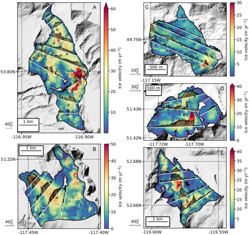
FIGURE 2. Surface velocity of (A) Conrad, (B) Illecillewaet, (C) Kokanee, (D) Nordic and (E) Zillmer glaciers. Velocity fields are 2018 mosaics of individual feature-tracking-derived velocity fields (Table 2). Flux gates are white lines and glaciological observations are white dots with black outline. Black arrows depict surface ice velocity vectors at the flux gates with variable scaling for visibility.

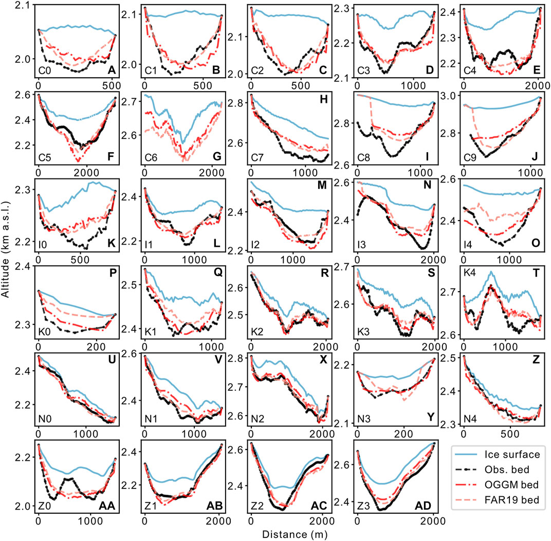
FIGURE 3. Flux gate cross-sections for (A–J) Conrad, (K–O) Illecillewaet, (P–T) Kokanee, Nordic (U–Z), and Zillmer (AA–AD) glaciers. Gates are numbered according to glacier, e.g., Conrad gate 0 = C0.

3.4 Surface Mass Balance

To calculate $b_a$ for each flux bin from our flux estimates, we quantify height change ($dh/dt$) and vertical ice velocity ($V_z$, which we use to describe both emergence and submergence velocity), while neglecting firn compaction ($V_{firn}$ = 0.0 m a⁻¹). Each component is expressed in meters of surface displacement per year. We use these components to calculate surface height change from mass balance (h, where $h=b_a/\rho$), which multiplied by density (ρ) of a given bin yields the $b_a$ of a given bin (j):

We use coregistered 1 m resolution DEMs collected via repeat fixed-wing ALS surveys to generate $dh/dt$ for each year from 2015 to 2018. ALS surveys average 1–3 laser shots m⁻² (Pelto et al., 2019). We assess height change uncertainty (${\sigma }_{dh/dt}$) over stable terrain after correction for effective sample size (Pelto et al., 2019), with an average ${\sigma }_{dh/dt}$ of 0.31 $\pm$ 0.10 m. Flux estimates (m³ a⁻¹) for each bin (Eq. 3) are normalized relative to the bin’s surface area $A_j$ (m²) to calculate $V_z$ (m a⁻¹).

While our primary analysis excludes firn compaction, we test including $V_{firn}$ in our mass-balance calculation (Eq. 4). Firn compaction is not considered in most geodetic studies because such studies primarily have multi-annual temporal scales (e.g., Tennant and Menounos, 2013; Magnússon et al., 2016; Zemp et al., 2013), and focus on glacier-wide mass balance where dynamic processes can be neglected. Even annual geodetic balance studies often neglect firn compaction (e.g., Pelto et al., 2019; Klug et al., 2018), as the required data input is onerous (e.g., Sold et al., 2013, 2015), the uncertainty high, and the net effect on mass balance small (Belart et al., 2017). We estimate $V_{firn}$ following the method of Sold et al. (2013) where over the cycle of one hydrological year and integrated over the whole firn column, one annual accumulation layer is transformed from snow to ice. For each flux bin with retained accumulation, we take the positive glaciological $b_a$ observations multiplied by the firn area of the particular bin. Mapping the area over which accumulation is continuously retained is difficult (Sold et al., 2015; Dunse et al., 2009), especially considering that firn area is shrinking on all five study glaciers, with multiple years of firn commonly exposed (Pelto et al., 2019). We merge all recent accumulation area masks (Pelto et al., 2019) from 2012 to 2018 (Figure 4) to best estimate the glacier area overlain with multi-year firn. We classify a given pixel as firn if covered by accumulation in $\ge$ 50% of the years. We take uncertainty on surface height change due to firn compaction (${\sigma }_{Vfirn}$) to be 10% (Pelto et al., 2019).

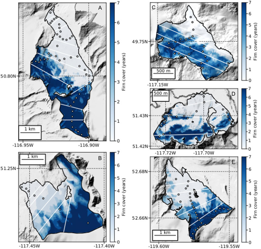
FIGURE 4. Accumulation area coverage derived from merging all recent accumulation area masks from 2012 to 2018 for (A) Conrad, (B) Illecillewaet, (C) Kokanee, (D) Nordic and (E) Zillmer glaciers. For a pixel with a value of seven, that pixel retained accumulation in all seven years. A value of zero implies a bare ice surface in all years. Flux gates are white lines and glaciological observations are white dots with black outline.

To estimate the mean density of each flux bin with retained accumulation (Figure 4), we use a firn model to estimate the density-depth relationship, which combined with the density of ice and mean ice thickness for the associated flux gate at the bottom of the bin, we estimate the mean column density of the flux bin. We use the Nabarro-Herring firn model (Arthern et al., 2010, Eq. 4), which we adapted from (Grinsted, 2021), fed with average annual temperature (Supplementary Figure 1), and average annual accumulation based on the nearest automatic snow weather station to each glacier (Supplementary Table 1) and a environmental lapse rate of −6.0 K km^-1. We scale firn column thickness by firn area for each bin (Figure 4). More details are in Supplementary Material 1.

We assess our modeled $b_a$ with our glaciological surface $b_a$ observations. The average number of annual balance measurement locations for each glacier are: Conrad, 38; Kokanee, 18; Illecillewaet, 8; Nordic, 22; and Zillmer 24 (Figure 2). See Pelto et al. (2019) for measurement details. We compare modeled flux-bin $V_z$ with $V_z$ as estimated at ablation stakes following Beedle et al. (2014) using an Eulerian framework and assuming that the measured ablation h at the stake is representative of a fixed position:

and $dh/dt$ is ALS height change sampled at the stake location. We compare modeled mass-balance gradients and flux-bin $b_a$ to observed gradients and $b_a$. Glaciological surface $b_a$ is calculated for each flux bin by taking the mean of all observations within a given bin. If there are less than two $b_a$ observations in a given bin, we select observations proximal to the bin with a search range that is 20% larger than the bin elevation range, if necessary incrementally increasing by 20% until the requirement is satisfied. We take uncertainty on glaciological $b_a$ as 0.26 m w.e., the average for these glaciers (Pelto et al., 2019).

We use mean error ($ME$) and mean absolute error ($MAE$) to compare flux-bin $b_a$ estimates to observations:

We assess the mass-balance profile by approximating the profile as a single linear function ($db/dz$), but also compare using a piecewise function comprised of two linear functions above ($d{b}^{+}/dz$) and below ($d{b}^{-}/dz$) the equilibrium line altitude (ELA) for Conrad and Nordic glaciers. No change in slope is detected for Kokanee, Illecillewaet or Zillmer glaciers when fit with a piecewise function. The ELA is the breakpoint for our piecewise functions (Furbish and Andrews, 1984; Malone et al., 2019). Uncertainties on balance gradients are taken as the standard error ($SE$) of the slope (Rabatel et al., 2005) for linear and piecewise functions. We chose linear and piecewise linear functions because of their wide application in glaciology (e.g., Kuhn, 1984; Rea, 2009) and their use in many models (e.g., Huss and Farinotti, 2012; Clarke et al., 2013).

We estimate the ELA by regressing modeled mass-balance. We compare these ELA to satellite-observations of the transient snow line (TSL), which we sample every 50 m. We estimate the satellite-ELA as the mean $\pm$ 1σ of these TSL samples. Because of the irregular nature of the retained accumulation on our glaciers (Figure 4), the σ of the satellite-ELA can be large.

3.5 Uncertainties

Systematic error in velocity can be assessed off-ice (e.g., Dehecq et al., 2019), and may stem from the cross-correlation itself, or DEM pre-processing. To assess systematic error, we quantify off-ice velocity, consider the uncertainty of the coregistration, and compare velocity fields against stake velocities. We assume coregistration accuracy of $\pm$2 pixels (Pelto et al., 2019). In the native resolution of the DEMs this equates to $\pm$2 m. Given that the average magnitude of off-ice velocity (<1.0 m a⁻¹) and the average difference between velocity fields and stake velocities ($\sim$1.4 m a⁻¹) are similar, this error and the error of coregistration are summed quadratically to derive systematic error (${\sigma }_{v_{syst}}$). Random error inherent in the cross-correlation and due to interannual variability is also estimated. Average displacement is roughly 5 pixels, and maximum displacement is 15–20 pixels in the fastest areas of flow. Thus most features do not show strong deformation and are easy to track. The accuracy of the cross-correlation is estimated to be $\pm$0.5 pixels, which corresponds to $\pm$1.5 m a⁻¹. This error, which also encompasses interannual variability, is taken as the random error. Random and systematic uncertainties combine to produce total ice velocity uncertainty (${\sigma }_v$):

While IPR observations are numerous, gaps in IPR data exist along some flux gates (Figure 3). We interpolate between the available measurements using a polynomial function (the degree of the polynomial function varies and is chosen to avoid overfitting i.e., unrealistic bed shapes) (Supplementary Figure 2), and where we interpolate, we assume an additional 10% uncertainty on ice thickness.

To calculate uncertainty in ice flux for a given gate (${\sigma }_{{\text{Φ}}_{gate}}$), we propagate the uncertainties of ice velocity and ice thickness in the ice flux equation (Berthier et al., 2003) summed for all segments (i) of the gate:

To address uncertainty in our depth-averaged velocity (we approximate depth-averaged velocity as 85% of surface velocity), we consider full slip (depth-averaged velocity is 100% of surface velocity) and no slip (depth-averaged velocity is 80% of surface velocity) to produce a ${\sigma }_{{\text{Φ}}_{gate}}$ for each velocity, and take the maximum ${\sigma }_{{\text{Φ}}_{gate}}$ (Young et al., 2020). For a given flux bin ${\sigma }_{\text{Φ}}$ from the gate at the top of the bin represents the uncertainty on flux in (${\sigma }_{{\text{Φ}}_{in}}$) and ${\sigma }_{\text{Φ}}$ from the gate at the bottom of the bin represents uncertainty on flux out (${\sigma }_{{\text{Φ}}_{out}}$). Combining uncertainties, we estimate ${\sigma }_{\text{Φ}}$ for the flux bin:

Uncertainty on ice column density is taken as 10%. Uncertainties on $dh/dt$, $\text{Φ}$, and $V_z$ are summed quadratically to estimate uncertainty on height change from mass balance ${\sigma }_h$ for each bin j and then to calculate uncertainty on modeled mass balance ${\sigma }_{b_a}$:

4 Results

4.1 Cross-Sectional Area

The ice thickness estimates from IPR, OGGM and FAR19 produce different cross-sectional areas and variable bed shapes (Figure 3). However, the ratios of cross-sectional area between adjacent gates have a median difference of 4.8% between the three sources. These ratios play a major role in the estimates of flux in and flux out for a given bin. IPR cross-sectional areas are, on average, 6.1 $\pm$ 8.7% larger than OGGM with a range of −2.3% to +22.8%. Relative to FAR19, cross-sectional area from IPR is 16.8 $\pm$ 11.2% greater for all five glaciers. The six lowest gates at Conrad Glacier have smaller IPR cross-sections than OGGM and FAR19, and greater IPR cross-sections for the three gates in the accumulation zone. This systematic difference is also evident between the model estimates, OGGM cross-sections for the lower gates are greater than FAR19 cross-sections, and smaller than FAR19 for the higher gates (Figure 3).

4.2 Surface and Vertical Ice Velocity

Average glacier-wide ice velocity for Conrad Glacier is 18.7 $\pm$ 0.4 m a⁻¹ (Figure 5) with a maximum of 95 m a⁻¹ within the upper ice fall (Figure 2). Illecillewaet Glacier average glacier-wide ice velocity is 13.3 $\pm$ 0.5 m a⁻¹ with a maximum of 65 m a⁻¹. Average glacier-wide ice velocity is 5.0 $\pm$ 0.3 m a⁻¹ for Kokanee Glacier with a maximum of 30 m a⁻¹. Nordic Glacier average glacier-wide ice velocity is 8.0 $\pm$ 0.3 m a⁻¹ with a maximum of 48 m a⁻¹. Average glacier-wide ice velocity is 8.1 $\pm$ 0.6 m a⁻¹ for Zillmer Glacier with a maximum of 42 m a⁻¹.

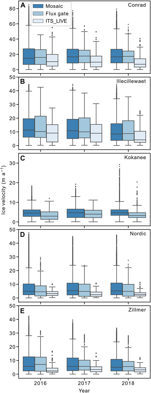
FIGURE 5. Surface ice velocity of each glacier from mosaics of our feature-tracking-derived annual velocity mosaics, for those mosaics as sampled along flux gates, and from ITS_LIVE annual mosaics. Boxplots depict 95% confidence interval (whiskers), interquartile (IQR) range (box), and median line.

The median and interquartile (IQR) range of our glacier-wide annual feature-tracking-derived velocity fields and those same velocity fields as sampled along the flux gates, are all within $\pm$10%. The ITS_LIVE median velocities fall near the bottom of the IQR range of our feature-tracking-derived velocities (Figure 5). Glacier-wide ITS_LIVE velocities are on average 39% slower than our estimates. For every glacier, the median surface velocity of each annual feature-tracking-derived velocity mosaic as sampled along the flux gates is typically within $\pm$ 10%. Average variability between each years’ mosaic is $\pm$ 4.0% and between each years’ mosaic and the three-year mosaic is $\pm$ 3.5%.

We find a mean difference between our 99 stake velocity pairs and feature-tracking velocity of 1.7 $\pm$ 0.51 m a⁻¹, and a median absolute difference of 3.2 m a⁻¹ (Figure 6). For Kokanee Glacier, stake velocities are less than feature-tracking velocities by 0.7 m a⁻¹. Stake velocities at Conrad, Nordic and Zillmer Glaciers are greater than feature-tracking velocities by 2.5 m a⁻¹. At Conrad Glacier, stakes close to the glacier margin along three transverse cross-sections of stakes have a larger median absolute difference (2.8 m a⁻¹) than those near the center (2.0 m a⁻¹).

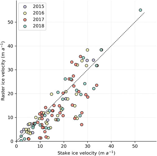
FIGURE 6. Surface ice velocity from 99 stake measurements on Conrad, Kokanee, Nordic and Zillmer glaciers vs. feature-tracking-derived velocity fields.

Flux-bin vertical ice velocities are generally between −2 and +3 m a⁻¹ (Figure 7). Vertical ice velocities estimated at ablation stakes and from modeled ice flux are visually similar, but a quantitative comparison is not attempted. The model estimates are for entire flux bins and not intended to produce point observations. Our greatest observed stake emergence velocity was +3.2 m a⁻¹, with a surface velocity of 47 m a⁻¹. Further details are in Supplementary Material 4.

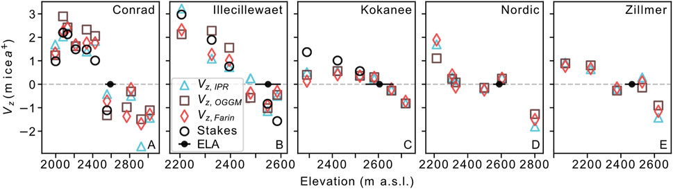
FIGURE 7. Vertical ice velocity from model estimates using the three ice thickness sources (IPR, OGGM, FAR19) and ablation stakes observations (Eq. 5), here averaged over the flux bins. The ELA is taken as the average ELA (defined here as the mean TSL elevation from satellite imagery at the end of the ablation season) from 2013 to 2018 $\pm$1σ.

4.3 Mass Balance

Modeled $db/dz$ are on average within $\pm$ 6.6% of observed $db/dz$, with a median difference between modeled and observed gradients of +7.6% (Table 3; Figure 8). Thirty-six of forty-five modeled $db/dz$ are within $\pm$ 1.0 $SE$ of observed $db/dz$ (Supplementary Tables 2–6). Six modeled $db/dz$ are outside $\pm$ 1.0 $SE$ at Zillmer Glacier. All modeled $db/dz$ are less steep than observed $db/dz$ for Kokanee Glacier, where three model $db/dz$ outside $\pm$ 1.0 $SE$ of observed $db/dz$ occur. If we instead use three-year mosaics of ice velocity rather than annual mosaics, modeled $db/dz$ only change by 1.6 $\pm$ 5.0% on average. For the four glaciers where it is available, using ITS_LIVE velocities decreases modeled $db/dz$ by 39% on average compared to our feature-tracking-derived velocities (Supplementary Figure 4). For piecewise linear functions for Conrad and Nordic glaciers, we find that the model estimates of $d{b}^{-}/dz$ were within $\pm$ 2% of observed on average, but that and $d{b}^{+}/dz$ are within $\pm$ 18% for Conrad Glacier and 45% for Nordic Glacier gradients (Figure 9). The median difference reveals that $d{b}^{-}/dz$ is three-times steeper than $d{b}^{+}/dz$ (Supplementary Tables 2–5). Variability of $d{b}^{+}/dz$ is greater than for $d{b}^{-}/dz$ for Conrad and Nordic glaciers, and the $SE$ values of $d{b}^{+}/dz$ are on average double those of $d{b}^{-}/dz$. Between the $b_a$ estimates from the three ice thickness sources, IPR produces $db/dz$ closer to observed $db/dz$ than OGGM or FAR19. FAR19 has the lowest $db/dz$ values for every glacier except Nordic Glacier. However, for the flux-bin $b_a$ estimates, FAR19 has slightly lower $ME$ and $MAE$ than OGGM or IPR (Table 3). Using Clarke et al. (2013) ice thickness we underestimate $db/dz$ at Conrad Glacier by 22.6% (Supplementary Figure 5) vs. $\pm$ 8% for modeled $db/dz$ from the other three sources. Regressing modeled mass balance, ELAs are on average 15 m higher than satellite-observations of ELA. Modeled ELAs are within 100 m 90% of the time. All ELA estimates outside 100 m of satellite observations occur at Zillmer Glacier in 2017, and Conrad Glacier in 2018.

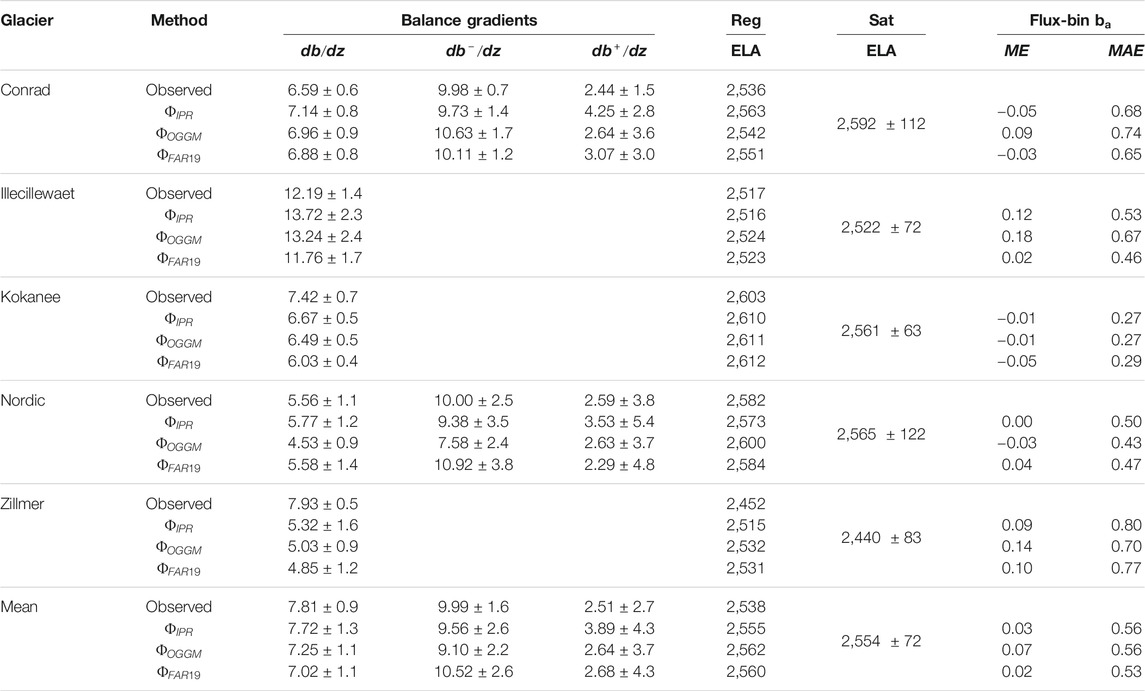
TABLE 3. Average mass-balance gradients (mm w.e. m⁻¹), regression-estimated ELA (Reg), satellite-estimated ELA (Sat), and flux-bin $b_{a}ME$ (m w.e.), and $MAE$ (m w.e.) for each glacier and for all glaciers collectively. Supplementary Tables 2–6 contain annual statistics for each glacier.

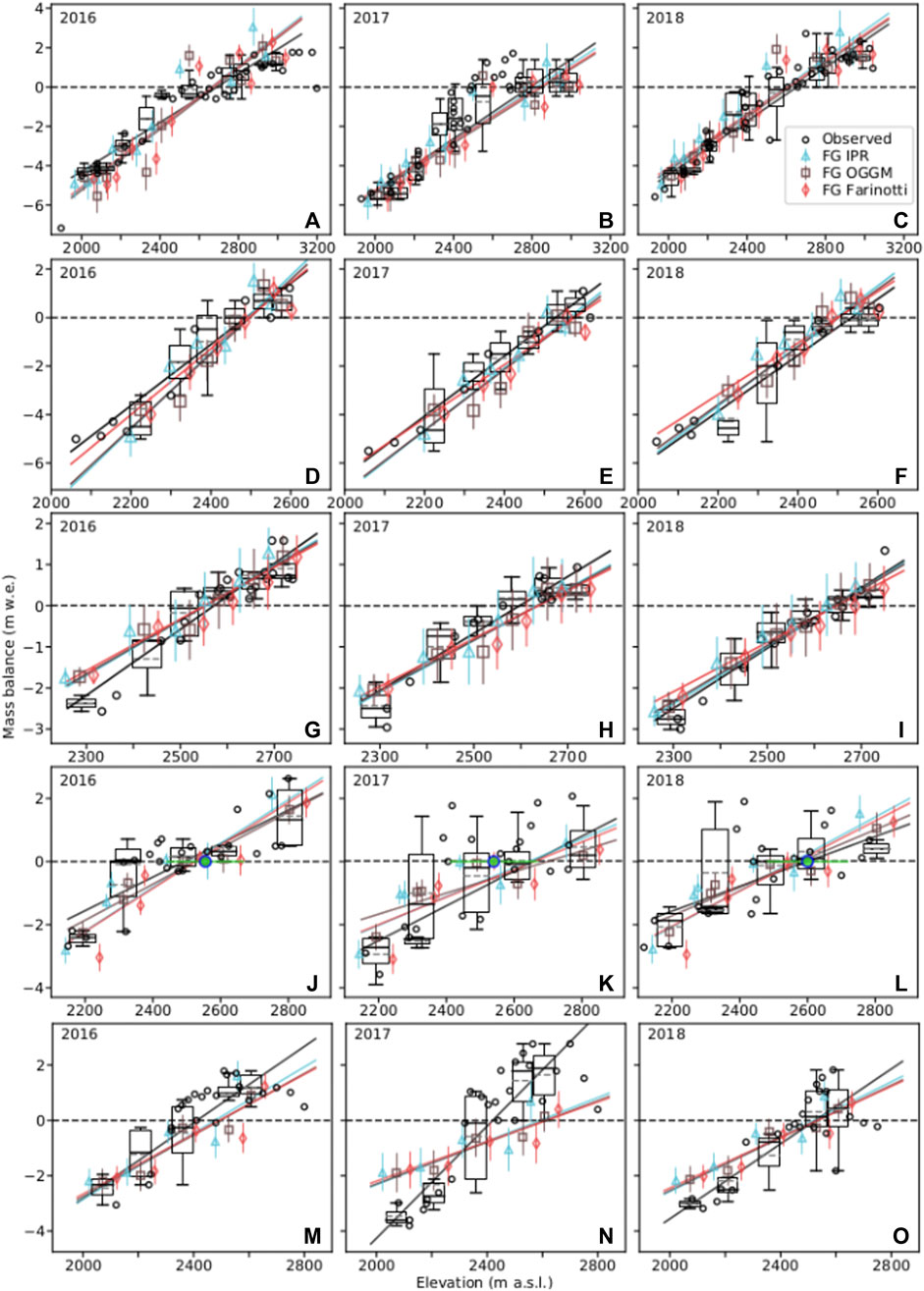
FIGURE 8. Observed and modeled (flux gate, FG) $b_a$ for Conrad (A–C), Illecillewaet (D–F), Kokanee (G–I), Nordic (J–L) and Zillmer (M–O) glaciers for 2016, 2017 and 2018. Balance gradients are fit with linear functions. Boxplots represent glaciological $b_a$ observations for each flux bin with 95% confidence interval (whiskers), IQR range (box), median (black line) and mean (dashed grey line). Colored error bars represent modeled $b_a$ for each flux bin.The ALS survey for Zillmer Glacier in 2017 occurred 74 days later than planned (Supplementary Figure 3).

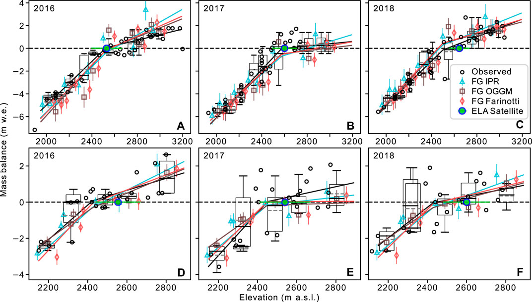
FIGURE 9. Observed and modeled (flux gate, FG) $b_a$ for Conrad (A–C), and Nordic (D–F) glaciers for 2016, 2017 and 2018. Data are the same as in Figure 8, but balance gradients are fit with piecewise linear functions. Boxplots represent glaciological $b_a$ observations for each flux bin with 95% confidence interval (whiskers), IQR range (box), median (black line) and mean (dashed grey line). Colored error bars represent modeled $b_a$ for each flux bin.

Comparing observed and modeled flux-bin $b_a$, we find an average $ME$ of +0.03 $\pm$ 0.07 m w.e. (Table 3) and an average $MAE$ of 0.55 $\pm$ 0.18 m w.e. If we instead use three-year mosaics of ice velocity rather than annual mosaics, $ME$ and $MAE$ increase slightly to 0.06 and 0.60 m w.e., respectively. Using ITS_LIVE velocities increases average $MAE$ to 0.85 m w.e. (Supplementary Figure 4). Using ice thickness from Clarke et al. (2013) increases error with a $ME$ and $MAE$ of −0.42 and 0.99 m w.e., respectively (Supplementary Figure 5). Resampled to 200 m, the resolution of Clarke et al. (2013) ice thickness, $MAE$ increases from our other ice thickness sources by 0.18 m w.e. The visual distribution of $b_a$ residuals (observed—modeled) around zero, best illustrated by the kernel density estimation in Figure 10, is encouraging. The kernel density estimation represents the probability distribution as a non-parametric estimator of density. A slight negative bias in modeled mass balance (positive $b_a$ residuals) appears over the middle elevations, but the mean residual between 0.3 and 0.8 normalized elevation where the kernel plot visualizes this bias is −0.004 $\pm$ 0.45 m w.e., with a $MAE$ of 0.63 m w.e. There is a slight positive bias over the lower elevations with an average residual of −0.20 m w.e. $\pm$ 0.55 m w.e. ANOVA tests between the binned $b_a$ observations and each of the three sets of modeled $b_a$ estimates across the three years for each glacier have an average p-value of 0.82, with a minimum p-value of 0.58 for the Conrad Glacier IPR-based $b_a$.

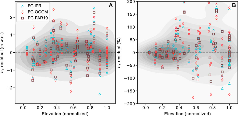
FIGURE 10. Mass-balance residuals (observed—modeled) for flux bins against normalized elevation for Conrad, Illecillewaet, and Kokanee glaciers. Residuals are expressed as (A) net residuals, and (B) percent residuals. All points are used for the kernel density estimation plot (grey) which represents the probability distribution as a non-parametric estimator of density. For (B), 40 large residuals $>\pm 200\text{\%}$ are not shown to better display the spread of most residuals (n = 294). These omitted percent residuals are predominately near the ELA, with a median normalized elevation of 0.75. The net magnitude of residuals is independent of elevation, but the percent residuals grow with increasing elevation as the net magnitude of mass balance decreases near and above the ELA relative to the lower elevations (Figure 8).

Our estimates of height change due to firn compaction range from 0.01 to 0.89 m a⁻¹ for specific bins. Including our estimate of firn compaction for flux bins which contain retained accumulation, our balance gradients are 10.6% steeper than without firnification. The inclusion of firn compaction slightly reduces error for modeled $db/dz$ for OGGM and FAR19, but increases $db/dz$ error for IPR, and greatly increases $d{b}^{+}/dz$ error for all three sources. Including firn compaction creates a positive flux-bin $b_a$ bias as indicated by $ME$ (−0.11 $\pm$ 0.07 m w.e). $MAE$ increases by 0.04 m w.e. to 0.59 m w.e. with firn compaction. Column-averaged-density is typically $>$850 kg m⁻³ in the accumulation zones, though most glaciers have a bin with a density around 815–840 kg m⁻³. Minimum density is typically high on the glaciers where accumulation is high, and thickness relatively low.

4.4 Uncertainty

We estimate ice velocity uncertainty (${\sigma }_v$) to be $\pm$ 2.7 m a⁻¹ (Eq. 8). Average ice velocity uncertainty (${\sigma }_v$) ranges from 15% for Conrad Glacier, to 55% for Kokanee Glacier, and averages 31%. Average ice flux uncertainty (${\sigma }_{\text{Φ}}$, Eq. 10), ranges from 19% for Conrad Glacier to 85% for Kokanee Glacier, and averages 41%. Average modeled ${\sigma }_{b_a}$ (Eq. 11) is 0.57 m w.e.

5 Discussion

5.1 Does Our Modeled Mass Balance Achieve Mass Conservation?

We consider mass to be conserved if the sum of h (glaciological balance height change) and modeled $V_z$ falls within $\pm$ 1σ of the ALS $dh/dt$ for a given bin during a given year (Berthier and Vincent, 2012). For 84% of bins, representing 86% of total glacier area, mass is conserved (Figure 11). The three ice thickness estimates all achieved similar mass conservation on average ($\pm$ 3%). We applied our GPS surveys to correct for mass change between data collection (Pelto et al., 2019), but fresh snow is difficult to resolve (Belart et al., 2017). In some cases, we suspect that insufficient data are responsible for mass conservation failure with either: 1) inadequate accumulation zone glaciological samples; 2) mass change between field and ALS surveys; or 3) insufficient LiDAR coverage. We further discuss these issues in Supplementary Material 3. Using field data to assess mass conservation can be problematic given the relatively sparse coverage of in situ measurements for some bins (Figure 2), and the time elapsed between ALS surveys and field observations. Ideally, mass balance would be modeled over the spatial extent of the bins (e.g., Berthier and Vincent, 2012), yet we consider this beyond the scope of our study. The relatively large terror on modeled mass balance may achieve mass conservation for some bins which have large mass-balance residuals. We thus consider our mass conservation assessment a first-order approximation.

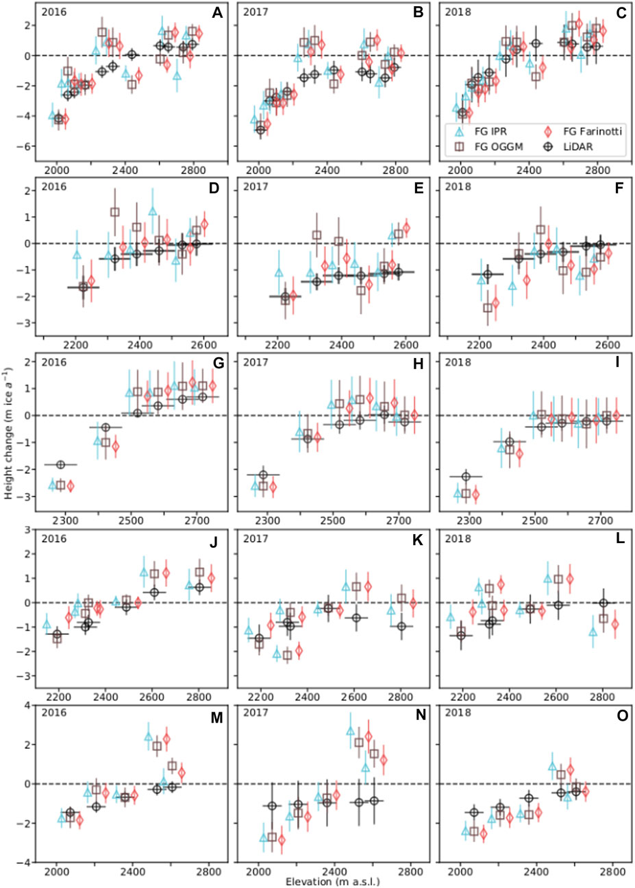
FIGURE 11. Mass conservation plot Conrad (A–C), Illecillewaet (D–F), Kokanee (G–I), Nordic (J–L) and Zillmer (M–O) glaciers for 2016, 2017, and 2018. The black error bars represent ALS-derived $dh/dt\pm {\sigma }_{dh/dt}$ for each flux bin. The colored error bars represent the sum of observed $b_a$ height change (h) and $V_z$ and, if mass conservation is respected, will equal the ALS $dh/dt$. This assumes that the ALS and field observations capture the glacier at the same time; Illecillewaet Glacier lacks GPS surveys to correct for height change between ALS and field surveys.

5.2 Can we Reliably Reproduce the Mass-Balance Profile From Remotely Sensed Data?

Our modeled gradients from all three ice thickness sources accord with observed gradients (Table 3). We chose single linear functions (Figure 8), and piecewise linear functions (Figure 9) to define balance gradients (Furbish and Andrews, 1984), however, $b_a$ estimates from our method can be used to directly describe the mass-balance profile (Kuhn, 1984), or fit with any desired function. The agreement among modeled balance gradients is interesting given the differences in cross-sectional area between the three sources (Figure 3). It is unsurprising that OGGM and IPR ice thicknesses produce greater cross-sectional area overall than does FAR19 since Pelto et al. (2020) found that observed ice thickness was underestimated by previous studies (Huss and Farinotti, 2012; Clarke et al., 2013; Farinotti et al., 2019). Similar balance gradients from the three ice thickness sources is likely due to consistent ratios of cross-sectional area between adjacent gates for ice flux estimates despite different bed shapes and cross-sectional areas.

Individual flux-bin $b_a$ do not perform as well as the gradients they produce. Average $ME$ (Table 3) is relatively low and $b_a$ residuals cluster around zero over the glacier elevation ranges (Figure 10), suggesting that the modeled estimates perform well in net, but large $MAE$ represents the variability of modeled $b_a$ observations. We do not find a systematic bias in modeled flux-bin $b_a$ relative to observations. Large ANOVA p-values between binned $b_a$ estimates from the different ice thickness implementations suggest that the differences between the means are not statistically significant. Errors in modeled mass balance (Supplementary Material 3) may stem from: 1) errors in ice flux; 2) sparse validation data ($b_a$); 3) gaps in ALS coverage; 4) differences in acquisition dates between ALS and glaciological surveys; 5) ice density used; or 6) firn compaction.

Our mass balance gradients are relatively insensitive to segmentation of the glacier (the number and location of flux gates), however, the flux bin estimates are sensitive to the segmentation. Using more gates we find that the altitude profile is more variable. Primary causes for this effect appear to be ice velocity sampling (e.g., adjacent gates on areas of faster flow and slower flow, respectively) and the effect of width scaling on cross-sectional area.

Including firn compaction steepens our mass balance gradients via an increase in accumulation zone $b_a$. Greater slope improves some $b_a$ gradients, overall improving the fit of $db/dz$ for OGGM and FAR19, but degrading that for IPR and of $d{b}^{+}/dz$ for all sources. IPR $db/dz$ was degraded due to the relatively larger mass balance estimated for some accumulation zone flux bins, where for a number of cross-sections, greater IPR thickness relative to OGGM and FAR19 (Figure 3 H–J, N, O, T) resulted in greater ice flux. Our rationale for excluding firn compaction is to demonstrate that this method can be used in the absence of glaciological observations, and because accurately determining firn compaction is challenging (e.g., Sold et al., 2015). Our method for estimating firn compaction requires knowledge of average accumulation from field observations and the spatial pattern of accumulation (Figure 4). This undermines our ability to estimate mass-balance gradients in the accumulation zones from remote data only. We also tested using the average annual compaction indicated by the firn model to estimate firn compaction, with similar results. The firn model compaction rates were larger than our compaction estimates, and steepened the gradients by 19%, increasing error. We further discuss firn compaction in Supplementary Material 1.

ITS_LIVE velocities systematically underestimate ice velocity (Figure 5). That our feature-tracking-derived ice velocities from 3 m resolution DEMs and optical satellite imagery are greater than those from ITS_LIVE is unsurprising, particularly for smaller glaciers with a large ratio of edge to interior pixels, yet the magnitude of the difference is surprising. Ice velocity and $db/dz$ (Supplementary Figure 4) both being 39% smaller relative to our velocities demonstrates how ice flux scales with ice velocity in a continuity approach, and the value of accurate velocity products. These differences hold up when sampled at ITS_LIVE resolution rather than our 25 m resolution (Supplementary Figure 3). The fit of $db/dz$ degrades for all glaciers with ITS_LIVE velocities (Supplementary Figure 4), however, the effect is smallest for the Conrad Glacier, which at 16.9 km² is much larger than the other glaciers (Table 1). ITS_LIVE multi-year mosaics performed worse than the annual ITS_LIVE mosaics. Our glaciers feature complex terrain and are irregular in dimension, producing radial flow that may be difficult for the resolution of ITS_LIVE. We suspect that for slightly larger glaciers, or glaciers with a simple geometry, velocity products like ITS_LIVE may be readily applicable. ITS_LIVE velocities worked well for a similar approach on the large (1,096 km²) Kaskawalush Glacier (Young et al., 2020).

Worse fit of $db/dz$ (Supplementary Figure 5) relative to the other ice thickness sources and increased error on $b_a$ estimates when using ice thickness data from Clarke et al. (2013), is likely in part due to underestimating ice thickness for these relatively small mountain glaciers (Pelto et al., 2020), but may also be due to lower resolution. Despite degrading the fit of $db/dz$, Clarke et al. (2013) ice thickness still produced gradients within $\pm$ 2.0 $SE$ of observations.

5.3 What Are the Primary Challenges to Flux Estimates of Mass Balance?

Challenges to calculate $b_a$via flux gates include the accuracy, coverage, and uncertainty of velocity fields, ice thickness, and surface topography. The number and representativeness of field measurements is important if assessing the accuracy of modeled $b_a$. Our results are sensitive to the quality of our ALS surveys. The worst model performance occurred at Zillmer Glacier in 2017 (Fig. 8N), with the ALS survey occurring on November 3, 2017, 74 days after the glaciological visit (Supplementary Material 3).

The relative influence of ${\sigma }_H$ and ${\sigma }_v$ on ${\sigma }_{\text{Φ}}$ (Eq. 9) varies by bin and glacier. ${\sigma }_v$ dominates uncertainty for gates with ice velocity below 10 m a⁻¹. Our ${\sigma }_H$ of 10.2% for the model estimates of H implies that ${\sigma }_H$ is smaller than ${\sigma }_v$ for most gates. For regional-scale studies, ${\sigma }_H$ is typically around 30% (Huss and Farinotti, 2012; Helfricht et al., 2019). Implementing our approach for glaciers without ice thickness observations would likely imply a greater ${\sigma }_H$ than reported here. In turn, percent ${\sigma }_v$ may need to be reduced relative to ours to achieve reasonable ${\sigma }_{\text{Φ}}$. This implies either improved velocity products or faster moving ice. With increased ${\sigma }_H$, smaller, slow-moving glaciers may have a prohibitively large ${\sigma }_{\text{Φ}}$ for accurate flux estimates. For faster moving ice, ${\sigma }_v$ is often $<$5–10% (Berthier et al., 2003; Berthier and Vincent, 2012; Burgess et al., 2013; Dehecq et al., 2019) which would decrease ${\sigma }_{\text{Φ}}$ substantially. As demonstrated by agreement between observed and modeled $db/dz$ for the five glaciers, modeled ice thicknesses from FAR19 and OGGM are of sufficient quality to represent the subglacial topography for estimates of mass balance for these glaciers.

Our velocity fields from individual image pairs reveals tolerable inter-annual variability in ice velocity but often contained data gaps (Table 2). Variability among individual velocity fields is likely due to the quality of the DEMs from variability in ALS point density, noise and artifacts in the velocity fields and data coverage, as much as to real changes in ice velocity. We chose to produce a mosaic of velocity fields for each year separately to best represent potential inter-annual variability, though find that the mean difference between the annual and three-year mosaics were minor and within uncertainties. Using a single velocity mosaic rather than annual mosaics only slightly increases $ME$ on modeled $b_a$. For relatively small mountain glaciers, velocity changes over short periods (e.g., three years) will typically be within velocity uncertainty, and a single ice velocity can be used to represent the period, as done by Vincent et al. (2021). Theoretically, the change in velocity due to creep from 4.95 m of thinning over the tongue of Conrad Glacier from 2016 to 2018 would yield a 2.5% decrease in velocity, well within our reported uncertainty of ice velocity. This expected slowdown due to reduced driving stress via thinning is important over longer periods (Dehecq et al., 2019). Our correction of modeled and observed ice thickness for thinning during our three-year study had a negligible effect on ice flux and $b_a$ estimates. With the current rate of thinning over the ablation zones of our glaciers, we would expect thinning to produce a change in velocity which would impact our flux-derived $b_a$ estimates after 5–10 years. Kokanee, Nordic and Zillmer glaciers demonstrate that glaciers or areas of glaciers with mean ice velocity less than 10 m a⁻¹ are challenging to measure, but possible with high resolution DEMs or imagery.

The limitation of our validation dataset is the sparse nature of our glaciological observations for some bins. Calculations of $b_a$ from glaciological observations are often biased due to uncaptured spatial variability (O’Neel et al., 2019; Zemp et al., 2013). We sampled the ablation zones of Conrad and Illecillewaet glaciers more densely than the accumulation zones (Figure 4). Pelto et al. (2019) found that the three transverse cross-sections of stakes in the ablation zone of Conrad Glacier show minor variability in $b_a$ whereas measurements in the accumulation zone show greater variability. The Fluctuations of Glaciers database also shows a bias toward ablation measurements, with a nearly 4 to 1 ratio of ablation to accumulation zone measurements (WGMS, 2018). Illecillewaet Glacier provides an example of this spatial bias where only 1–2 measurements are made above 2,500 m, representing 75% of its area. Further discussion of mass balance is in Supplementary Material 3.

5.4 Can This Method Be Expanded?

Farinotti et al. (2019) (FAR19) produced globally distributed ice thickness maps and we suggest that they can be used to represent ice thickness to estimate $b_a$ from ice flux. The success of OGGM and FAR19 relative to IPR demonstrates that modeled ice thickness can adequately represent cross-sectional ice area, or at least represent the ratio of cross-sectional area for adjacent flux-gates, for ice-flux derived $b_a$ estimates for some mountain glaciers. Ice velocity estimates are becoming increasingly widespread and accurate (Heid and Kääb, 2012; Burgess et al., 2013; Dehecq et al., 2019; Gardner et al., 2020), suggesting that velocity can be reasonably determined for many glaciers. While ITS_LIVE velocities were not successful here for most years, we emphasize that our glaciers have complex topography and geometries, and are relatively small, so suggest that ITS_LIVE velocities, or similar resolution products, may perform well for glaciers with simpler geometry and in particular, for larger, faster flowing glaciers (e.g., Young et al., 2020). When extending a mass-continuity approach over accumulation zones, we recommend estimating firn column depth and density to inform total ice column density, and find this to be more important than accounting for firn compaction. For either approach, firn column depth or firn compaction must be scaled by firn area, otherwise modeled mass balance will be biased. We acknowledge that our relative success may stem from the availability of high-resolution geodetic data, which may not be available for other studies. We suspect that lower resolution data (e.g., Brun et al., 2017; Dussaillant et al., 2019) could perform well in our framework, particularly if used for larger glaciers, or if the mass-balance profile is aggregated from tens or hundreds of glaciers. If high resolution data truly are a prerequisite for success with a continuity approach, this would still increase the number of glaciers for which mass balance gradients are estimated from tens or hundreds (Rea, 2009; WGMS, 2018) to thousands or tens of thousands given the growing availability of high-resolution data (e.g., Shean et al., 2016, 2020; Belart et al., 2017; Klug et al., 2018; Pelto et al., 2019). Annual remote sensing elevation data are becoming increasingly common (e.g., Klug et al., 2018; Pelto et al., 2019; Shean et al., 2020), though most such datasets are often still nearer decadal scale (e.g., Zemp et al., 2013; Magnússon et al., 2016). While we employed a flux-gate method, if well-distributed velocity estimates are available, a gridded method (e.g., Mcnabb et al., 2012) or a full-stokes ice flow model (e.g., Jarosch, 2008) could also be used.

Recent efforts to remotely estimate surface mass balance are limited but growing (Bisset et al., 2020; Gao et al., 2020; Young et al., 2020; Vincent et al., 2021). Some of these approaches resolve point mass-balance but require data inputs which render them more suitable for individual glaciers (Young et al., 2020), or specific areas of individual glaciers (Vincent et al., 2021). Vincent et al. (2021) derive point surface mass balances from vertical ice velocities and surface elevation change. Their method estimates point surface mass balance, and demonstrates the potential for expanding the limited number of point observations of surface mass balance available globally, but relies upon an assumption of constant vertical ice velocities and requires a dense network of in situ observations, which limits application of their approach in space and time. Young et al. (2020) use a fully distributed mass-balance model driven by downscaled and bias-corrected climate-reanalysis data, requiring spatially distributed glacio-meteorological data (e.g., reanalysis products, weather station timeseries, in situ accumulation and ablation measurements). Their approach is best suited to quantify the mass budget of individual glaciers, particularly large, regionally significant glaciers. Remote-sensing-based mass-continuity approaches, like the one employed here and by Bisset et al. (2020), may be readily scaled up, and should expand the number of glaciers for which the mass balance-altitude relation can be quantified, providing model validation (of balance gradients) in a framework like that of OGGM (Maussion et al., 2019).

6 Conclusion

We use a mass-conservation approach to quantify the distribution of surface mass balance of five alpine glaciers over three years in the Columbia Mountains of BC, using an extensive dataset of field and remote-sensing observations. We quantify elevation change with annual 1 m resolution ALS DEMs. Our feature-tracking-derived velocity fields and three ice thickness sources, both modeled and observed, estimate ice fluxes through cross-sections. Our modeled mass-balance gradients ($db/dz$) fit well with observed $db/dz$ with an average difference of $\pm$ 6.6%. Our modeled flux-bin $b_a$ have low $ME$ (+0.03 $\pm$ 0.07 m w.e.), but high variability (average $MAE$ 0.55 $\pm$ 0.18 m w.e.). Regression of our flux-bin $b_a$ produce reasonable ELA estimates. For our glaciers, ITS_LIVE velocities are 39% lower than our velocity fields, and produce worse $db/dz$ fit and larger $ME$ and $MAE$. Despite varying cross-sectional areas, the three ice thickness sources yield similar ratios of cross-sectional area between adjacent gates, with a median difference of 4.5%. According to our first-order approximation, mass conservation is respected for 84% of flux bins representing 86% of total glacier area.

Reasonable fit of modeled and observed $db/dz$ and relatively small $b_a$ residuals over accumulation zones, despite neglecting firn compaction, demonstrates success in extending the flux gate method over the entire elevation range of alpine glaciers. The performance of modeled ice thicknesses within our method, relative to observations, indicates that representing the ratio of cross-sectional area between adjacent gates, is more important for flux-derived mass-balances than achieving ice thicknesses which “exactly” match true ice thicknesses. For our relatively small alpine glaciers, ice velocity represents greater uncertainty than ice thickness for most flux bins. Given the availability of velocity software and products (e.g., Shean et al., 2016; Gardner et al., 2020), global estimates of ice thickness (Farinotti et al., 2019), and modern elevation data (e.g., Brun et al., 2017), estimating ice flux to derive mass balance is likely feasible for many glaciers.

Data Availability Statement

The datasets presented in this study can be found in online repositories. The names of the repository/repositories and accession number(s) can be found below: The ice penetrating radar data used in this study can be found in the Glacier Thickness Database (GlaThiDa, https://www.gtn-g.ch/data_catalogue_glathida/). The glacier mass balance data can be found in the Fluctuations of Glaciers (FoG) Database (WGMS, 2018). Point observations of mass balance, DEMs, and ice velocity products are all available by request. Code used for the analyses can be found at https://github.com/bpelto/continuity_flux.

Author Contributions

Both authors contributed to the development of the research question and general conceptual approach. BP wrote all code, conducted the analyses and led the writing and production of the manuscript. Both authors reviewed and edited the manuscript.

Funding

This research was supported by the Canadian Columbia Basin Glacier and Snow Research Network (CCBGSRN) with funding from Columbia Basin Trust, BC Hydro, Tula Foundation, the Natural Sciences and Engineering Research Council of Canada, Canada Foundation for Innovation and Canada Research Chairs Program. Funding for BP was provided via a Pacific Institute for Climate Solutions fellowship, the University of Northern British Columbia, and the Columbia Basin Trust.

Conflict of Interest

The authors declare that the research was conducted in the absence of any commercial or financial relationships that could be construed as a potential conflict of interest.

Acknowledgments

We are grateful for the insightful feedback provided by Gwenn Flowers and BP’s committee members Shawn Marshall, Peter Jackson, Stephen Déry, and Roger Wheate. We thank Planet for access to their excellent imagery though their Ambassador program. We thank reviewers Evan Miles and Ellyn Enderlin and the Scientific Editor, Alun Hubbard, for providing detailed reviews that substantially improved our manuscript.

Supplementary Material

The Supplementary Material for this article can be found online at: https://www.frontiersin.org/articles/10.3389/feart.2021.675681/full#supplementary-material

References

Arthern, R. J., Vaughan, D. G., Rankin, A. M., Mulvaney, R., and Thomas, E. R. (2010). In Situ measurements of Antarctic Snow Compaction Compared with Predictions of Models. J. Geophys. Res. 115, F03011. doi:10.1029/2009jf001306
CrossRef Full Text | Google Scholar
Bach, E., Radić, V., and Schoof, C. (2018). How Sensitive Are Mountain Glaciers to Climate Change? Insights from a Block Model. J. Glaciol. 64, 247–258. doi:10.1017/jog.2018.15
Beedle, M. J., Menounos, B., and Wheate, R. (2014). An Evaluation of Mass-Balance Methods Applied to Castle Creek Glacier, British Columbia, Canada. J. Glaciol. 60, 262–276. doi:10.3189/2014JoG13J091
Belart, J. M. C., Berthier, E., Magnússon, E., Anderson, L. S., Pálsson, F., Thorsteinsson, T., et al. (2017). Winter Mass Balance of Drangajökull Ice Cap (NW Iceland) Derived from Satellite Sub-meter Stereo Images. The Cryosphere 11, 1501–1517. doi:10.5194/tc-11-1501-2017
Berthier, E., Raup, B., and Scambos, T. (2003). New Velocity Map and Mass-Balance Estimate of Mertz Glacier, East Antarctica, Derived from Landsat Sequential Imagery. J. Glaciol. 49, 503–511. doi:10.3189/172756503781830377
Berthier, E., Vincent, C., Magnússon, E., Gunnlaugsson, Á. Þ., Pitte, P., Le Meur, E., et al. (2014). Glacier Topography and Elevation Changes Derived from Pléiades Sub-meter Stereo Images. The Cryosphere 8, 2275–2291. doi:10.5194/tc-8-2275-2014
Berthier, E., and Vincent, C. (2012). Relative contribution of surface mass-balance and ice-flux changes to the accelerated thinning of Mer de Glace, French Alps, over1979-2008. J. Glaciol. 58, 501–512. doi:10.3189/2012JoG11J083
Bisset, R. R., Dehecq, A., Goldberg, D. N., Huss, M., Bingham, R. G., and Gourmelen, N. (2020). Reversed Surface-Mass-Balance Gradients on Himalayan Debris-Covered Glaciers Inferred from Remote Sensing. Remote Sensing 12, 1563. doi:10.3390/rs12101563
Bolch, T., Menounos, B., and Wheate, R. (2010). Landsat-based Inventory of Glaciers in Western Canada, 1985-2005. Remote Sensing Environ. 114, 127–137. doi:10.1016/j.rse.2009.08.015
Brun, F., Berthier, E., Wagnon, P., Kääb, A., and Treichler, D. (2017). A Spatially Resolved Estimate of High Mountain Asia Glacier Mass Balances from 2000 to 2016. Nat. Geosci 10, 668–673. doi:10.1038/ngeo2999
PubMed Abstract | CrossRef Full Text | Google Scholar
Burgess, E. W., Forster, R. R., and Larsen, C. F. (2013). Flow Velocities of Alaskan Glaciers. Nat. Commun. 4, 2146. doi:10.1038/ncomms3146
Clarke, G. K. C., Anslow, F. S., Jarosch, A. H., Radić, V., Menounos, B., Bolch, T., et al. (2013). Ice Volume and Subglacial Topography for Western Canadian Glaciers from Mass Balance fields, Thinning Rates, and a Bed Stress Model. J. Clim. 26, 4282–4303. doi:10.1175/JCLI-D-12-00513.1
Clarke, G. K. C., Jarosch, A. H., Anslow, F. S., Radić, V., and Menounos, B. (2015). Projected Deglaciation of Western Canada in the Twenty-First century. Nat. Geosci 8, 372–377. doi:10.1038/ngeo2407
Cogley, J. G., Hock, R., Rasmussen, L., Arendt, A., Bauder, A., Braithwaite, R., et al. (2011). Glossary of Glacier Mass Balance and Related Terms, IHP-VII Technical Documents in Hydrology No. 86, IACS Contribution No. 2. Paris: International Hydrological Program, UNESCO, 114.
Cuffey, K. M., and Paterson, W. S. B. (2010). The Physics of Glaciers. fourth edn.. Burlington, MA: Elsevier.
Dehecq, A., Gourmelen, N., Gardner, A. S., Brun, F., Goldberg, D., Nienow, P. W., et al. (2019). Twenty-first century Glacier Slowdown Driven by Mass Loss in High Mountain Asia. Nat. Geosci 12, 22–27. doi:10.1038/s41561-018-0271-9
Dunse, T., Schuler, T. V., Hagen, J. O., Eiken, T., Brandt, O., and Høgda, K. A. (2009). Recent Fluctuations in the Extent of the Firn Area of Austfonna, Svalbard, Inferred from GPR. Ann. Glaciol. 50, 155–162. doi:10.3189/172756409787769780
Dussaillant, I., Berthier, E., Brun, F., Masiokas, M., Hugonnet, R., Favier, V., et al. (2019). Two Decades of Glacier Mass Loss along the Andes. Nat. Geosci. 12, 802–808. doi:10.1038/s41561-019-0432-5
Farinotti, D., Huss, M., Bauder, A., Funk, M., and Truffer, M. (2009). A Method to Estimate the Ice Volume and Ice-Thickness Distribution of alpine Glaciers. J. Glaciol. 55, 422–430. doi:10.3189/002214309788816759
Farinotti, D., Huss, M., Fürst, J. J., Landmann, J., Machguth, H., Maussion, F., et al. (2019). A Consensus Estimate for the Ice Thickness Distribution of All Glaciers on Earth. Nat. Geosci. 12, 168–173. doi:10.1038/s41561-019-0300-3
Frey, H., Machguth, H., Huss, M., Huggel, C., Bajracharya, S., Bolch, T., et al. (2014). Estimating the Volume of Glaciers in the Himalayan-Karakoram Region Using Different Methods. The Cryosphere 8, 2313–2333. doi:10.5194/tc-8-2313-2014
Furbish, D. J., and Andrews, J. T. (1984). The Use of Hypsometry to Indicate Long-Term Stability and Response of valley Glaciers to Changes in Mass Transfer. J. Glaciol. 30, 199–211. doi:10.3189/S0022143000005931
Gao, H., Zou, X., Wu, J., Zhang, Y., Deng, X., Hussain, S., et al. (2020). Post-20th century Near-Steady State of Batura Glacier: Observational Evidence of Karakoram Anomaly. Sci. Rep. 10, 987. doi:10.1038/s41598-020-57660-0
Gardner, A. S., Fahnnestock, M. A., and Scambos, T. A. (2020). ITS_LIVE Regional Glacier and Ice Sheet Surface Velocities. Data archived at National Snow and Ice Data Center. doi:10.5067/6II6VW8LLWJ7
GlaThiDa, (2019). Glacier Thickness Database 3.0.1. World Glacier Monitoring Service, Zurich, Switzerland. doi:10.5904/wgms-glathida-2019-03
Grinsted, A. (2021). Steady State Snow and Firn Density Model. Available at: https://www.mathworks.com/matlabcentral/fileexchange/47386-steady-state-snow-and-firn-density-model (Accessed March29 2021).
Google Scholar
Gudmundsson, G. H., and Bauder, A. (1999). Towards an Indirect Determination of the Mass-Balance Distribution of Glaciers Using the Kinematic Boundary Condition. Geografiska Annaler A 81, 575–583. doi:10.1111/j.0435-3676.1999.00085.x
Heid, T., and Kääb, A. (2012). Repeat Optical Satellite Images Reveal Widespread and Long Term Decrease in Land-Terminating Glacier Speeds. The Cryosphere 6, 467–478. doi:10.5194/tc-6-467-2012
Helfricht, K., Huss, M., Fischer, A., and Otto, J.-C. (2019). Calibrated Ice Thickness Estimate for All Glaciers in Austria. Front. Earth Sci. 7, 68. doi:10.3389/feart.2019.00068
Hubbard, A., Willis, I., Sharp, M., Mair, D., Nienow, P., Hubbard, B., et al. (2000). Glacier Mass-Balance Determination by Remote Sensing and High-Resolution Modelling. J. Glaciol. 46, 491–498. doi:10.3189/172756500781833016
Huss, M., and Farinotti, D. (2012). Distributed Ice Thickness and Volume of All Glaciers Around the globe. J. Geophys. Res. 117, F04010–n. doi:10.1029/2012JF002523
Jarosch, A. H. (2008). Icetools: A Full Stokes Finite Element Model for Glaciers. Comput. Geosciences 34, 1005–1014. doi:10.1016/j.cageo.2007.06.012
Kääb, A., and Funk, M. (1999). Modelling Mass Balance Using Photogrammetric and Geophysical Data: a Pilot Study at Griesgletscher, Swiss Alps. J. Glaciol. 45, 575–583. doi:10.3189/S0022143000001453
Klug, C., Bollmann, E., Galos, S. P., Nicholson, L., Prinz, R., Rieg, L., et al. (2018). Geodetic Reanalysis of Annual Glaciological Mass Balances (2001-2011) of Hintereisferner, Austria. The Cryosphere 12, 833–849. doi:10.5194/tc-12-833-2018
Kuhn, M. (1984). Mass Budget Imbalances as Criterion for a Climatic Classification of Glaciers. Geografiska Annaler: Ser. A, Phys. Geogr. 66, 229–238. doi:10.1080/04353676.1984.11880111
Magnússon, E., Muñoz-Cobo Belart, J., Pálsson, F., Ágústsson, H., and Crochet, P. (2016). Geodetic Mass Balance Record with Rigorous Uncertainty Estimates Deduced from Aerial Photographs and Lidar Data - Case Study from Drangajökull Ice Cap, NW Iceland. The Cryosphere 10, 159–177. doi:10.5194/tc-10-159-2016
Malone, A. G. O., Doughty, A. M., and Macayeal, D. R. (2019). Interannual Climate Variability Helps Define the Mean State of Glaciers. J. Glaciol. 65, 508–517. doi:10.1017/jog.2019.28
Maussion, F., Butenko, A., Champollion, N., Dusch, M., Eis, J., Fourteau, K., et al. (2019). The Open Global Glacier Model (OGGM) v1.1. Geosci. Model. Dev. 12, 909–931. doi:10.5194/gmd-12-909-2019
Mcnabb, R. W., Hock, R., O’Neel, S., Rasmussen, L. A., Ahn, Y., Braun, M., et al. (2012). Using Surface Velocities to Calculate Ice Thickness and Bed Topography: a Case Study at Columbia Glacier, Alaska, USA. J. Glaciol. 58, 1151–1164. doi:10.3189/2012JoG11J249
Meier, M. F., and Post, A. S. (1962). Recent Variations in Mass Net Budgets of Glaciers in Western North America. IAHS Publ. 58, 63–77.
O'Neel, S., McNeil, C., Sass, L. C., Florentine, C., Baker, E. H., Peitzsch, E., et al. (2019). Reanalysis of the US Geological Survey Benchmark Glaciers: Long-Term Insight into Climate Forcing of Glacier Mass Balance. J. Glaciol. 65, 850–866. doi:10.1017/jog.2019.66
Oerlemans, J., and Hoogendoorn, N. C. (1989). Mass-Balance Gradients and Climatic Change. J. Glaciol. 35, 399–405. doi:10.3189/S0022143000009333
Pelto, B. M., Maussion, F., Menounos, B., Radić, V., and Zeuner, M. (2020). Bias-corrected Estimates of Glacier Thickness in the Columbia River Basin, Canada. J. Glaciol. 66, 1051–1063. doi:10.1017/jog.2020.75
Pelto, B. M., Menounos, B., and Marshall, S. J. (2019). Multi-year Evaluation of Airborne Geodetic Surveys to Estimate Seasonal Mass Balance, Columbia and Rocky Mountains, Canada. The Cryosphere 13, 1709–1727. doi:10.5194/tc-13-1709-2019
Pfeffer, W. T., Arendt, A. A., Bliss, A., Bolch, T., Cogley, J. G., Gardner, A. S., et al. (2014). The Randolph Glacier Inventory: A Globally Complete Inventory of Glaciers. J. Glaciol. 60, 537–552. doi:10.3189/2014JoG13J176
Rabatel, A., Dedieu, J.-P., and Vincent, C. (2005). Using Remote-Sensing Data to Determine Equilibrium-Line Altitude and Mass-Balance Time Series: Validation on Three French Glaciers, 1994-2002. J. Glaciol. 51, 539–546. doi:10.3189/172756505781829106
Rabatel, A., Sanchez, O., Vincent, C., and Six, D. (2018). Estimation of Glacier Thickness from Surface Mass Balance and Ice Flow Velocities: A Case Study on Argentière Glacier, France. Front. Earth Sci. 6, 112. doi:10.3389/feart.2018.00112
Rabatel, A., Sirguey, P., Drolon, V., Maisongrande, P., Arnaud, Y., Berthier, E., et al. (2017). Annual and Seasonal Glacier-wide Surface Mass Balance Quantified from Changes in Glacier Surface State: A Review on Existing Methods Using Optical Satellite Imagery. Remote Sensing 9, 507. doi:10.3390/rs9050507
Radić, V., and Hock, R. (2011). Regionally Differentiated Contribution of Mountain Glaciers and Ice Caps to Future Sea-Level Rise. Nat. Geosci 4, 91–94. doi:10.1038/ngeo1052
Rea, B. R. (2009). Defining Modern Day Area-Altitude Balance Ratios (AABRs) and Their Use in Glacier-Climate Reconstructions. Quat. Sci. Rev. 28, 237–248. doi:10.1016/j.quascirev.2008.10.011
Rounce, D. R., Hock, R., and Shean, D. E. (2020). Glacier Mass Change in High Mountain Asia through 2100 Using the Open-Source Python Glacier Evolution Model (PyGEM). Front. Earth Sci. 7, 331. doi:10.3389/feart.2019.00331
Shean, D. E., Alexandrov, O., Moratto, Z. M., Smith, B. E., Joughin, I. R., Porter, C., et al. (2016). An Automated, Open-Source Pipeline for Mass Production of Digital Elevation Models (DEMs) from Very-High-Resolution Commercial Stereo Satellite Imagery. ISPRS J. Photogrammetry Remote Sensing 116, 101–117. doi:10.1016/j.isprsjprs.2016.03.012
Shean, D. E., Bhushan, S., Montesano, P., Rounce, D. R., Arendt, A., and Osmanoglu, B. (2020). A Systematic, Regional Assessment of High Mountain Asia Glacier Mass Balance. Front. Earth Sci. 7, 363. doi:10.3389/feart.2019.00363
Shean, D. E. (2019). Dshean/vmap: Zenodo DOI Release (v1.0.0). doi:10.5281/zenodo.3243479
Sold, L., Huss, M., Eichler, A., Schwikowski, M., and Hoelzle, M. (2015). Unlocking Annual Firn Layer Water Equivalents from Ground-Penetrating Radar Data on an alpine Glacier. The Cryosphere 9, 1075–1087. doi:10.5194/tc-9-1075-2015
Sold, L., Huss, M., Hoelzle, M., Andereggen, H., Joerg, P. C., and Zemp, M. (2013). Methodological Approaches to Infer End-Of-winter Snow Distribution on alpine Glaciers. J. Glaciol. 59, 1047–1059. doi:10.3189/2013JoG13J015
Tennant, C., and Menounos, B. (2013). Glacier Change of the Columbia Icefield, Canadian Rocky Mountains, 1919-2009. J. Glaciol. 59, 671–686. doi:10.3189/2013JoG12J135
Vallon, M., Vincent, C., and Reynaud, L. (1998). Altitudinal Gradient of Mass-Balance Sensitivity to Climatic Change from 18 Years of Observations on Glacier d'Argentière, France. J. Glaciol. 44, 93–96. doi:10.3189/S0022143000002380
Vincent, C., Cusicanqui, D., Jourdain, B., Laarman, O., Six, D., Gilbert, A., et al. (2021). Geodetic point Surface Mass Balances: A New Approach to Determine point Surface Mass Balances from Remote Sensing Measurements. The Cryosphere 1–30. doi:10.5194/tc-2020-239
Vincent, C., Soruco, A., Six, D., and Le Meur, E. (2009). Glacier Thickening and Decay Analysis from 50 Years of Glaciological Observations Performed on Glacier d'Argentière, Mont Blanc Area, France. Ann. Glaciol. 50, 73–79. doi:10.3189/172756409787769500
WGMS (2018). Fluctuations of Glaciers Database. Zurich, Switzerland: World Glacier Monitoring Service. doi:10.5904/wgms-fog-2018-11
CrossRef Full Text
Young, E. M., Flowers, G. E., Berthier, E., and Latto, R. (2020). An Imbalancing Act: the Delayed Dynamic Response of the Kaskawulsh Glacier to Sustained Mass Loss. J. Glaciol. , 67, 313. doi:10.1017/jog.2020.107
Zemp, M., Thibert, E., Huss, M., Stumm, D., Rolstad Denby, C., Nuth, C., et al. (2013). Reanalysing Glacier Mass Balance Measurement Series. The Cryosphere 7, 1227–1245. doi:10.5194/tc-7-1227-2013
Keywords: ice flux, glacier mass balance, ice velocity, flux gate, ice thickness, balance gradient, geodetic mass balance
Citation: Pelto BM and Menounos B (2021) Surface Mass-Balance Gradients From Elevation and Ice Flux Data in the Columbia Basin, Canada. Front. Earth Sci. 9:675681. doi: 10.3389/feart.2021.675681
Received: 03 March 2021; Accepted: 30 June 2021;
Published: 19 July 2021.
Edited by:
Alun Hubbard, Aberystwyth University, United Kingdom
Reviewed by:
Evan Stewart Miles, Swiss Federal Institute for Forest, Snow and Landscape Research (WSL), Switzerland
Ellyn Mary Enderlin, University of Maine, United States
Copyright © 2021 Pelto and Menounos. This is an open-access article distributed under the terms of the Creative Commons Attribution License (CC BY). The use, distribution or reproduction in other forums is permitted, provided the original author(s) and the copyright owner(s) are credited and that the original publication in this journal is cited, in accordance with accepted academic practice. No use, distribution or reproduction is permitted which does not comply with these terms.
*Correspondence: Ben M. Pelto, ben.pelto@ubc.ca