Coupled Source-Sink Habitats Produce Spatial and Temporal Variation of Cancer Cell Molecular Properties as an Alternative to Branched Clonal Evolution and Stem Cell Paradigms

Introduction

Regional variations in the molecular properties of cancer cells have been well established and are usually ascribed to accumulation of genetic changes, often called branched evolution, as each mutation initiates a new species (Fisher et al., 2012; Gerlinger et al., 2012; Zhang et al., 2019). This conceptual model is built upon the gene centric view of evolution, summarized as “mutation-selection,” in which cancer cells experience random mutations at a rate higher than normal cells and each mutation is then subject to selection by the overall tumor environment. Though most mutations are deleterious, the rare mutation that increases fitness will allow increased proliferation producing a genetically distinct subpopulation and, therefore, observable regional genotypic variations.

However, this paradigm (Archetti, 2013; Scott and Marusyk, 2017; Hinohara and Polyak, 2019) tends to neglect the role of spatio-temporal heterogeneity in environmental selection forces as a driver of evolution. In general, the fitness of any cancer cell is defined by the interaction of its phenotype with local environmental conditions. As conditions change in space so will the optimal phenotype of the cancer cells. Thus, natural selection may favor genetically and molecularly distinct cancer cells phenotypically suited to the local habitat type. But, these local habitat-specific cancer cell populations are not completely isolated. They are connected and more or less coupled through migration, the dispersal of individuals between habitats (Figure 1). Here we explore migration as a previously unrecognized driver of intra-tumoral evolution (Winker, 2000).

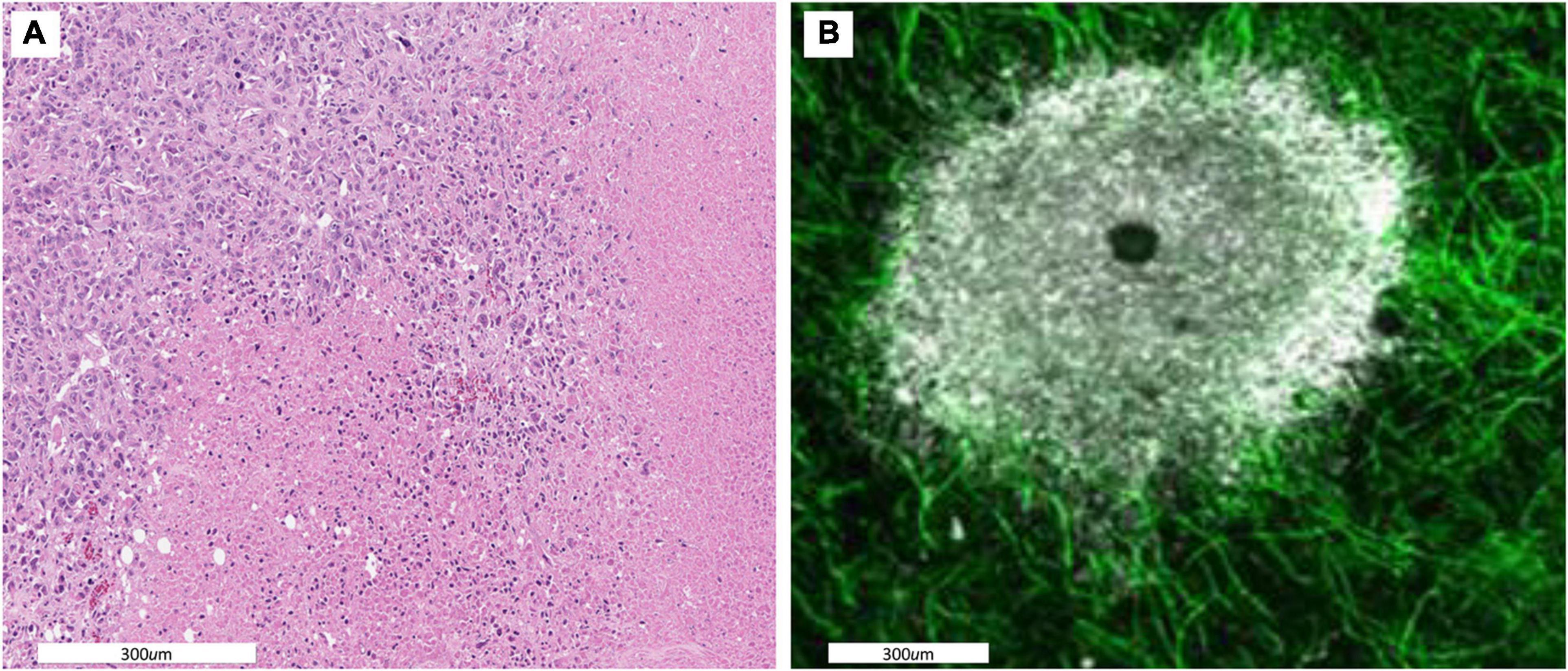
Figure 1. (A) A histological section showing spatial variations in intratumoral habitats. Cellular density is high in the upper left indicating a well perfused tumor region. The lower and right side of the images shows regions in which most cells are necrotic indicating little perfusion. (B) A dorsal window chamber view of a tumor grown in a mouse expressing endothelial GFP. Tumor cells are shown in white. As with the histological staining there is a clear well perfused vascular edge with a less dense avascular internal region and a necrotic core. Migration rates of ∼ 5 to 10 μm/h allow for individual cells to traverse within and between these habitats.

Initially described by Pulliam (1988), local movement of individuals can connect adjacent habitats with very different properties. For example, a “source habitat” has favorable environmental conditions and, therefore, a positive per capita population growth rate. Within tumors, a source habitat might be one that is well perfused with a large carrying capacity. In contrast, a “sink habitat” has unfavorable environmental conditions in which net mortality exceeds reproduction resulting in a higher within-habitat death than birth rate. In tumors, this would correspond to a region with little or no blood flow resulting in environmental conditions that, in the absence of migration, supports few if any cancer cells. When physically adjacent, these disparate habitats can be coupled through migration; and, within these metapopulations, a large fraction of individuals may reside in habitats that are, in the absence of migration, insufficient to maintain a net positive growth rate. Furthermore, consistent movement between habitats may alter the evolution of cancer cell phenotype resulting in habitat specialization or a single generalist cancer cell type whose adaptations balance exposure to both habitats (Holt and Gomulkiewicz, 1997).

In nature, it has been demonstrated, both theoretically (Brown and Pavlovic, 1992) and empirically (Boughton, 1999), that source-sink dynamics can act both spatially (Holt, 1985) and temporally (Johnson, 2004) to profoundly influence regional metapopulations residing in and moving between different habitats (Gravel et al., 2010). In particular, migration between habitats can result in speciation and subsequent co-existence of multiple different species. Thus, in addition to mutation, genetic drift and natural selection, evolutionary ecologists have come to recognize migration as a significant evolutionary force (Brown and Pavlovic, 1992). As noted by Brown and Pavlovic (1992) “when viewed as a property of the environment rather than a force of evolution, migration becomes part of the circumstances to which evolution by natural selection responds.”

Within tumors, the ability of individual cells to migrate (typically ∼ 5 to 10 μm/h) is recognized as a critical phenotypic adaptation for survival and cancer progression (Yamaguchi et al., 2005; Polacheck et al., 2013; Te Boekhorst et al., 2016; Paul et al., 2017; Staneva et al., 2019)). Migration is typically associated with epithelial-to-mesenchymal transition, wherein the latter phenotype is motile (Dongre and Weinberg, 2019). Once it arrives at a novel location or tissue, the cell can undergo the reverse: a mesenchymal to epithelial transition. Furthermore, the cancer stem-cell paradigm (Li et al., 2007; Walcher et al., 2020; Wang et al., 2020) posits a stem cell niche from which non-stem cells migrate (i.e., phenotypically distinct and not self-replicating) into adjacent tumor regions (Borovski et al., 2011). Here we note that “stem cells” may indeed be cells that occupy a source habitat and migration of these cells into a sink habitat produces both the phenotypic variation and reduced proliferative capacity described in the stem cell paradigm.

The specific source-sink dynamics depend highly on the characteristics of the sink environment. A black-hole or hard-sink habitat cannot sustain a viable population in the absence of continued immigration. Regardless of population size, in a hard sink, the individuals will experience a negative per capita growth rate. Within tumors, this would correspond to a region with little or no blood flow resulting in environmental conditions with a carrying capacity that is near zero. Migration from the source habitat can maintain a population within the sink habitat. The existence of multiple microscopic clusters of viable cells within macroscopic “necrotic” areas of tumors is well known in pathology (Jardim-Perassi et al., 2019). Hard sink habitats can provide some return migrants to the source habitat, influencing evolution, and even ecologically rescuing a source habitat from a catastrophic perturbation (Holt et al., 2004).

Alternatively, the less favorable habitat may act as a “soft” sink, which can support a viable population, albeit one that is much smaller than the source habitat. Asymmetries in population sizes or migration rates means that more individuals move from the richer habitat to the poorer than vice-versa. Under density dependent population growth, this means the system equilibrates to a steady state in which the source habitat is underpopulated (below its carrying capacity) and the sink habitat is overpopulated (above its carrying capacity). Source and sink habitats may exert selection for quite different phenotypic and genotypic properties; so much so that there is a potential for speciation and diversification (Cure et al., 2017).

We propose source-sink dynamics contribute to the spatial variability in molecular properties of cancer cells observed within and between tumors in the same patient. Some regions of a tumor and regions of the body represent hard sinks in which a dispersing cancer cell faces near immediate death upon arrival. For example, circulating tumor cells may extravasate (exit the circulating system) into a tissue totally unsuitable for survival so that a metastases never forms. Within the tumor, necrotic zones provide a hard sink. Examples of soft sink habitats may include poorly vascularized tumor regions or perhaps inflamed but otherwise normal tissue at the tumor edge.

Here, we illustrate the eco-evolutionary dynamics associated with source sink dynamics in black-hole, hard- and soft-sink circumstances. We focus on how migration into a sink habitat influences 1) local and total population sizes, 2) possible extinction of the entire population, 3) evolution of a trait that influence fitness in both the source and sink habitats, 4) speciation under conditions of a soft-sink habitat, and 5) eco-evolutionary responses to therapy that target the source habitat or the predominant cancer cell type. Results from goals 1–4 will be familiar to those familiar with the expansive literature on source sink dynamics (Diffendorfer, 1998). We demonstrate how source-sink dynamics are applicable to cancers and can produce the observed spatial variations in genetic and phenotypic properties of cancer cells, and suggest critical issues in designing patient treatment strategies.

Materials and Methods

Here, we model a source habitat and consider three variations of an adjacent sink habitat: a black-hole sink, a hard sink, and a soft sink (Gravel et al., 2010; Borovski et al., 2011; Gerlinger et al., 2012). In all cases the source habitat will generally be A and the sink B. When habitat B is a black hole sink, any cancer cell that migrates from A to B dies instantly. When habitat B is a hard sink, cancer cells cannot proliferate but they may die off slowly at some fixed per capita rate. When habitat B is a soft sink, it can sustain a smaller population of cancer cells than habitat A and becomes a sink habitat only because of the disproportionate number of migrants into B than out of B.

Within habitat A and within habitat B when it is a soft sink, cancer cells directly compete for space and limited resources. While these cancer cells do not directly compete with cells in the other habitat, they interact indirectly due to the dispersal of cancer cells between the source and sink regions. This dispersal is represented by a per capita migration rate that describes the probability that an individual in one habitat migrates to the other. This migration rate can also represent the habitat shifting underneath stationary cancer cells, such as when vasculature becomes unstable, shifting the boundary between well perfused and poorly perfused microenvironments.

The competition of cancer cells within a habitat and migration between habitats is analyzed using a game theoretic approach in which a G function couples ecological (population) and evolutionary (strategy) dynamics (Vincent and Brown, 2005). This framework is built upon the three principles of Darwin’s theory of natural selection: there must be heritable variation, there must be a “struggle for existence” (i.e., limited resources and space prevent all populations from growing exponentially), and heritable variation must influence this struggle. In the G function approach, one considers a focal (or virtual) cell with strategy (= heritable phenotype), v, which, along with the strategies (u) and densities (N_A,N_B) of competing cancer cell populations, determines the cell’s expected fitness or proliferation rate. For example, u may represent expression levels of key proteins implicated in cellular proliferation. Here, we let u = (u₁,…u_n) be the vector of strategies of the n different species where u_i represents the strategy of species i = 1,…,n. Note that the length of this vector can change dynamically in time: as species diversify or go extinct, the vector will correspondingly expand or shrink. Here, we assume that species are identical except for the values of their strategies. Let $N_A=(N_A^1,\mathrm{\dots },N_A^n)$ and $N_B=(N_B^1,\mathrm{\dots },N_B^n)$ be the vector of population sizes in the source habitat A and the sink habitat B, where $N_A^i$ represents the population size of species i in habitat A. Let F_A and F_B describe the fitness of a cancer cell in the source (A) and sink habitats (B), respectively. We assume that fitness within a habitat is only influenced by the cells within that habitat where F_A(v,u,N_A) and F_B(v,u,N_B).

We assume random migration between the two habitats where m_A is the per capita migration rate of cells from habitat A to habitat B, and vice versa for m_B. We assume these migration rates are constant but this could be relaxed to include density-dependent habitat selection (Rosenzweig, 1981; Tarjuelo et al., 2017) and migration rates themselves could become a component of the heritable strategy (Morris, 1991; Schmidt et al., 2000). The number of cells in the source increases as the source cells proliferate, and through incoming migration from the sink. The number of cells in the source decreases due to outgoing migration to the sink. These dynamics also apply, respectively to the sink. The change in population size of each habitat can be written as:

To simulate the eco-evolutionary dynamics of cancer cells, we treat our habitats as different states in the life history of cancer cells, coupled via migration. This framework allows us to capture the population dynamics of cancer cells with a population projection matrix. Each entry in the matrix represents transitions between the two life history states. An ecologically inclined reader may notice that this is analogous to the Leslie matrix for structured populations. Our population projection matrix, denoted by P, can be written as:

Then, we can represent our population dynamics as

Though we can use this matrix to simulate population dynamics, we must still construct a fitness function to capture strategy dynamics. We can define this fitness function as the dominant eigenvalue of the population projection matrix since this is what controls (approximates) long-term behavior (Vincent et al., 1993; Vincent and Brown, 2002). In other words, we have

where λ_i are the eigenvalues of P. Then, the evolutionary dynamics of u_i depends on the local gradient of the G function: how the fitness of the cells change due to perturbations in the trait value and the rate at which cells can climb this fitness gradient. Mathematically, the evolutionary dynamics of species i can be formalized (Vincent et al., 1993) as:

where c is a measure of additive genetic variance, in accordance with Fisher’s fundamental theorem of natural selection. The $\frac{\partial G}{\partial u}$ term captures the local gradient of the fitness generating function at v=u_i. To reiterate, a cell’s fitness, G(v,u,N_A,N_B), depends on its own strategy, v, the strategies of the other tumor cells, u, and the population sizes of tumor cells in the source habitat (A) and the sink habitat (B), N_A and N_B. The fitness generating function, G, describes the ecological (changes in total and local population size,N_A,N_B), and $\frac{\partial G}{\partial u}$ describes the evolutionary dynamics (changes in the populations heritable strategy values, u). If at v=u_i, G(v,u,N_A,N_B) = 0 then $N_A^i$ and $N_B^i$, the total population size of species i, will increase and vice-versa for G < 0. The direction of the strategy dynamics can be seen by the adaptive landscape which plots G versus the focal cell’s strategy, v, while holding the other cells’ strategies (u) and population densities (N_A,N_B) constant. A species strategy u_i will climb the adaptive landscape until the system reaches a stable point where it is both evolutionarily (∂G/∂u|_{v = ui} = 0) and ecologically stable ($\partial N_A^i/\partial t=\partial N_B^i/\partial t=0$). As u,N_A,N_B change, so too does the entire adaptive landscape, sometimes dramatically (Vincent and Brown, 2005).

We now consider the eco-evolutionary outcomes when the system starts with just a single species: n=1. Interestingly, the eco-evolutionary stable point can occur at either a minimum or a maximum of the adaptive landscape (Cohen and Brown, 1999). If the stable point is at a maximum of the landscape where (∂²⁡G/∂⁡u² < 0), the cancer cells have evolved to their evolutionary stable strategy (ESS) (Vincent and Brown, 1988). On this other hand, if the stable point is at a minimum of the landscape (∂²⁡G/∂⁡u² > 0), the cancer cells might speciate (= evolutionary branching, Geritz et al., 1998), creating two distinct cancer cell types or “species” each with its own unique strategy u₁ and u₂. These species will climb to their respective peaks of the adaptive landscape to reach their own unique ESS. Hence, when there is just one species: u=u₁ and $N_A=N_A^1,N_B=N_A^1$. When there are more than one species u,N_A,N_B becomes vector valued. Each species will have its own strategy and its own population distribution between the source and sink habitats.

The habitat-specific population dynamics $\frac{d{N}_A}{dt}$ and $\frac{d{N}_B}{dt}$, and habitat-specific fitnesses F_A and F_B, for the black-hole sink, hard sink, and soft sink are described in Box 1. We set r_A = r_B = 0.025 (many patient’s tumors experience growth at rates of 2.5 % per day) as the maximum growth rate of each habitat. The functional forms for carrying capacities and death rates are provided in Box 1. The strategy of the focal cell, v, influences either its habitat-specific carrying capacity or habitat-specific death rate: K_A(v), K_B(v), and d_B(v). For the relationships between K_A(v) and K_B(v) and v, we use a quadratic equation. The parabolas were scaled so that at v = 1,K_A(1) = 100 (maximum achievable carrying capacity in habitat A) and K_B(1) = 25 (the less well perfused habitat can support just 1/4 as many cells when the cells are best adapted for A). At v=0 (best adapted for habitat B), we let both habitats have the same carrying capacity of 50: K_A(0) = K_B(0) = 50. Thus, as v goes from 0 to 1 the cancer cell’s carrying capacity in habitat A goes from 50 to 100, and its carrying capacity in habitat B declines from 50 to 25 (Figure 2).

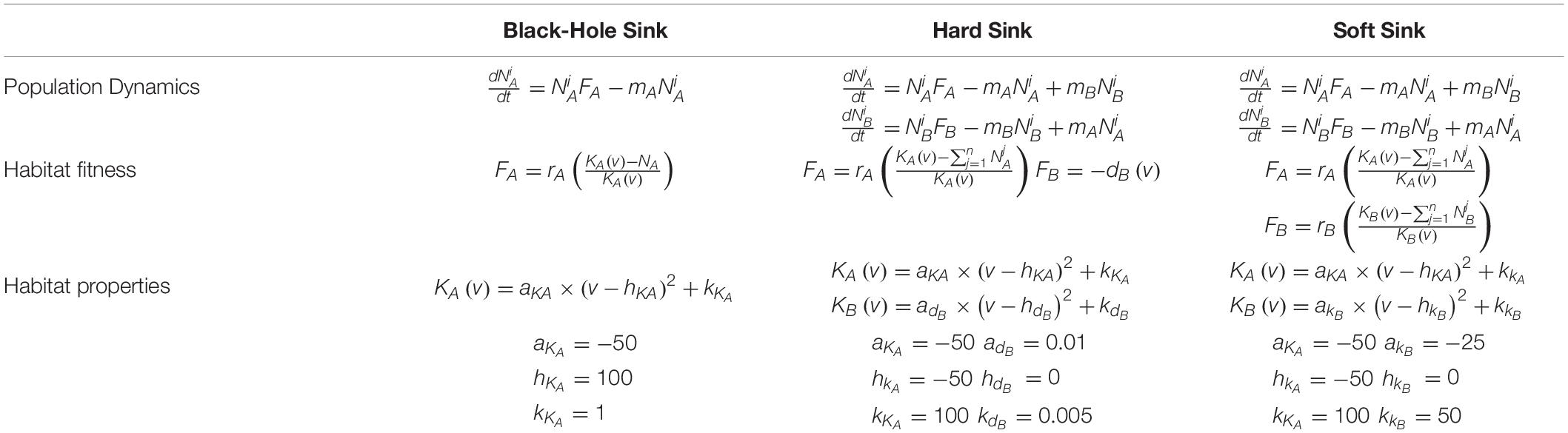
Box 1. Mathematical model of all three sink habitat scenarios including the population dynamics, habitat fitness functions, and the properties of the habitats with respect to a cell’s strategy.

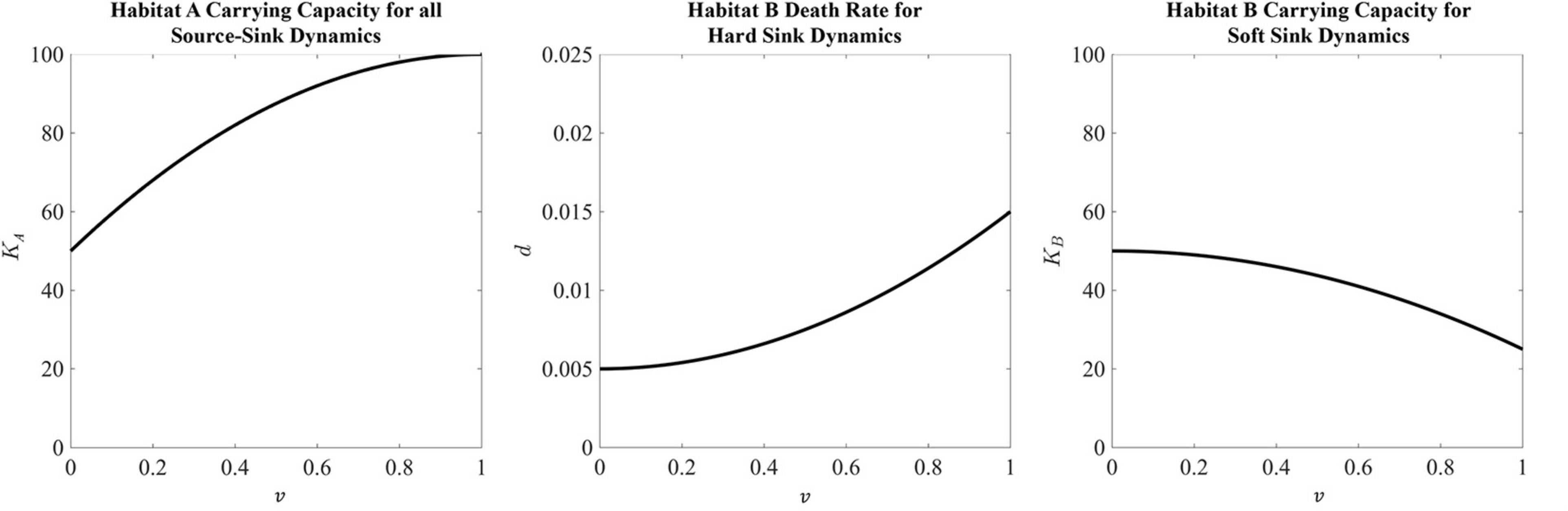
Figure 2. Habitat properties for the source and sink habitats defined in Box 1. The source habitat, which is the same for all three sink habitat analyses, has a maximum carrying capacity at a strategy equal to 1. This carrying capacity then falls as the strategy moves away from strategy value 1 toward a minimum carrying capacity of 50 with a strategy equal to 0. For the hard sink dynamics, habitat B is defined by a death rate. Here the death rate is minimized at a strategy equal to 0. This death rate increases at the strategy moves away from 0 to a maximum death rate of 0.015 at a strategy equal to 1. Lastly, the carrying capacity of the soft sink habitat B has a maximum of 50 at a strategy equal to 0. As the strategy moves toward 1, the carrying capacity falls to a value of 25.

To determine the effects of migration on the dynamics of the evolutionary game, we numerically solved for the ESS. We consider values for m_A and m_B in the range from very slow migration (m_A = m_B = 10⁻⁴) to very fast migration (m_A = m_B = 10⁰). We initialize each numerical run of the model by assuming that the cancer cells originate primarily in the source habitat A. In this way, we set the population density in habitat A to relatively full, N_A(0) = 95, habitat B to relatively empty N_B(0) = 5, and all cells with the strategy that maximizes fitness in habitat A, v=1 at time zero.

Modeling Treatment

The models for the black-hole, hard and soft sinks in Box 1 determine the cancer’s ecological and evolutionary dynamics in the absence of patient treatment. Within the context of the soft-sink model, we consider two types of treatment, habitat dependent and cancer cell phenotype dependent. Habitat dependent treatments are more effective in the source habitat than the sink habitat and have been previously modeled (Fu et al., 2015; Moreno-Gamez et al., 2015). In cancer, chemotherapeutic drugs perfuse more thoroughly through regions near the vasculature (source habitat) than habitats farther from vasculature (sink habitat). The diffusion dynamics that reduce nutrient concentrations away form blood vessels also reduces the concentration of systemically delivered drugs (Perez-Velazquez and Rejniak, 2020).

We additionally present a model for phenotype dependent treatment, where drug efficacy depends on the strategy of the cancer cells. This represents a targeted therapy that is maximally effective for a given strategy value and drug efficacy then declines as the cancer cells’ strategy deviates from the therapeutically optimal value.

To consider a habitat-dependent treatment, we add a death term that represents a habitat-specific therapy-induced death rate:

where γ_x represents the fraction of cells that die due to treatment in habitats A and B. We set γ_A = 0.05 and γ_B = 0 due to the increased delivery of drug to the well vascularized source habitat.

We model strategy dependent treatment as:

where γ(u) captures how effective the treatment is as a function of the cancer cell strategy, v. Specifically, we use the following form for γ(v):

where γ_M represents maximal drug efficacy set here to 0.05, v_opt is the cancer cell strategy at which the drug is maximally effective (v=1), and σ_t is a measure of how “general” the treatment is set here to 0.05. As the cancer cell’s strategy deviates from v_opt, drug efficacy declines according to a Gaussian curve. Figure 3 depicts the shape of this functional form.

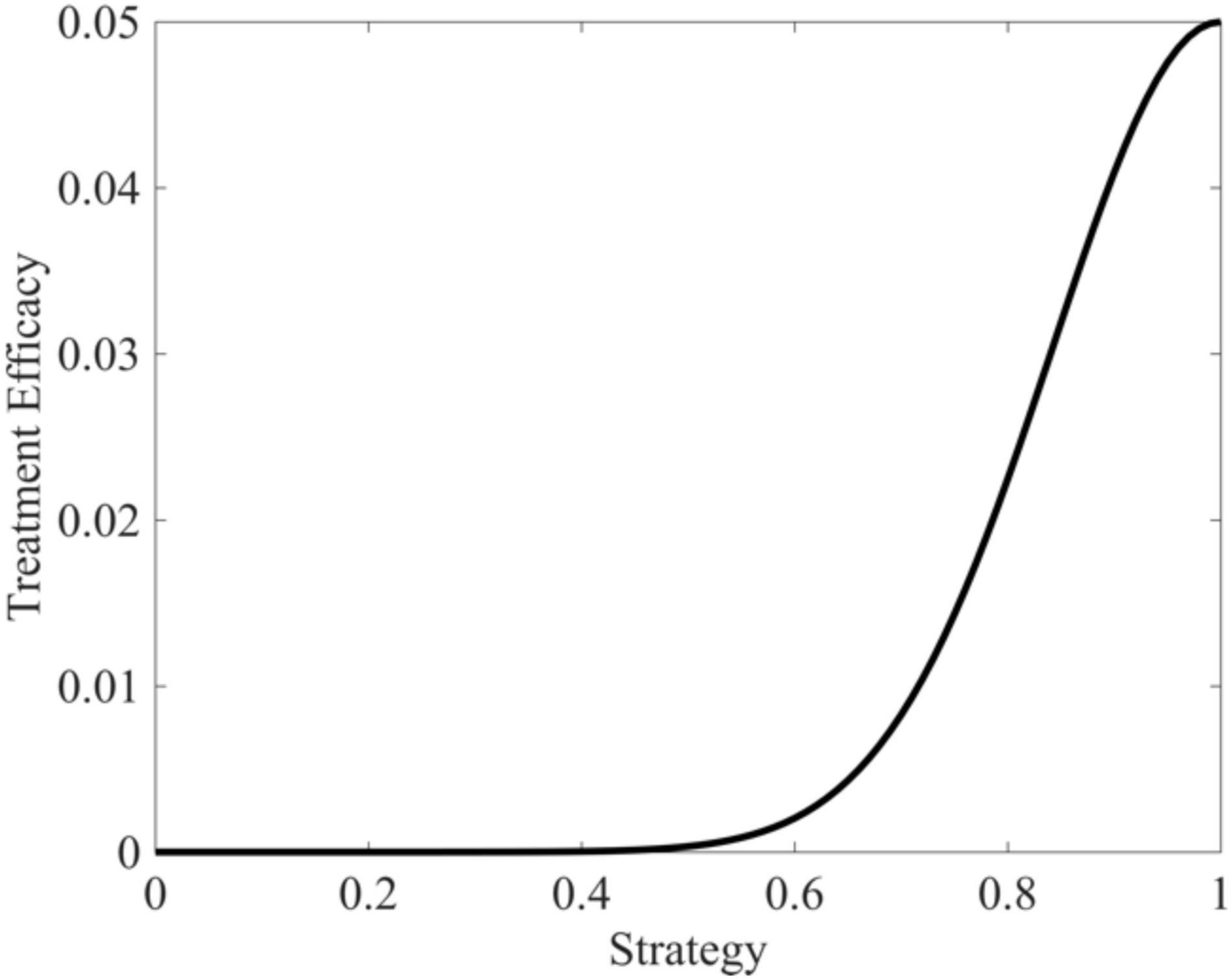
Figure 3. Targeted therapy efficacy as a function of trait value. Therapeutic efficacy is maximized when v = 1 and drops off in a Gaussian fashion as trait values diverge from v = 1.

Results

Black-Hole Sink

The black hole sink supports no population. From the perspective of the source population, migration to the black-hole sink represents a per capita death rate, shown in Figure 4. From the perspective of the cancer patient, any movement of cancer cells into surrounding tissue or extravasation of CTCs into completely inhospitable tissues is beneficial.

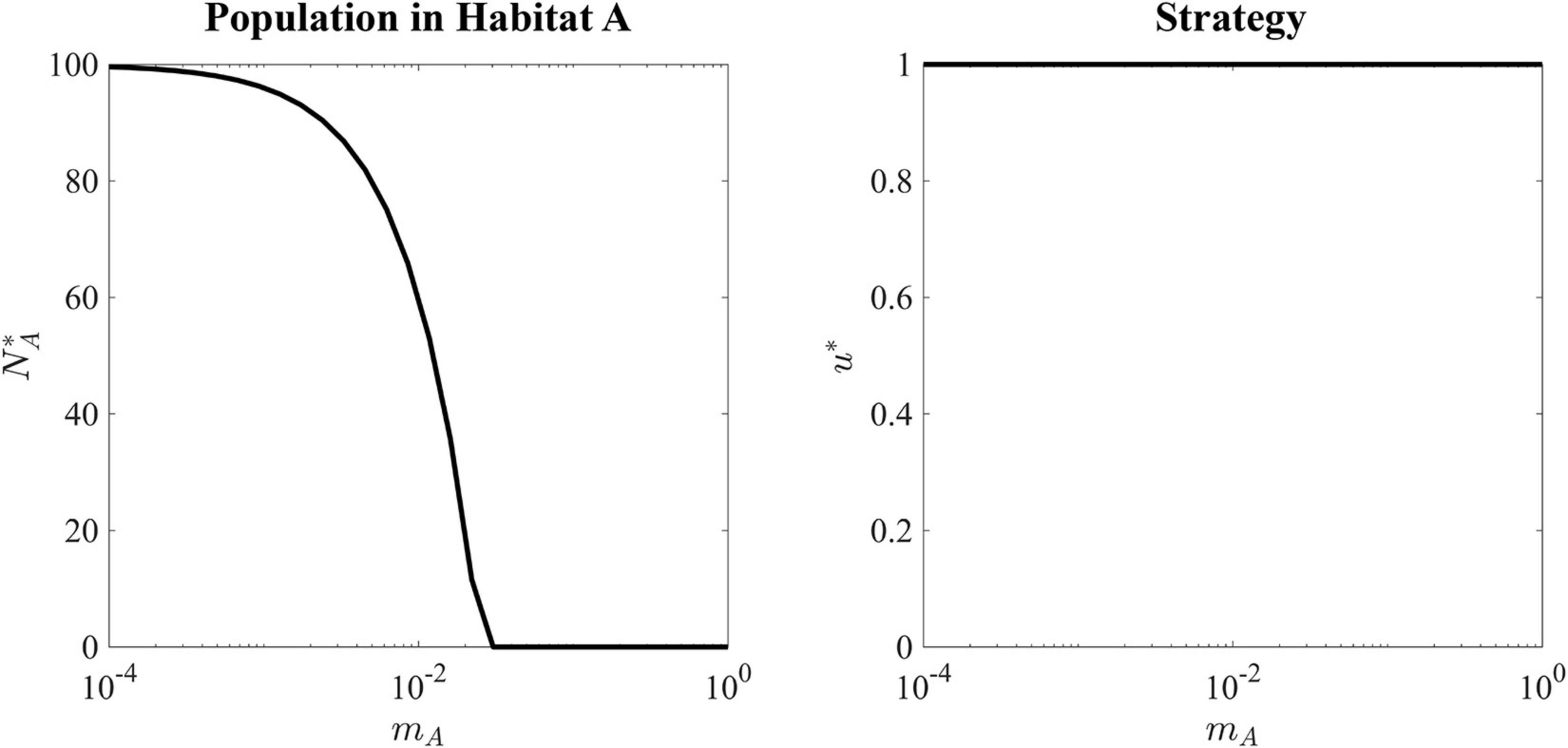
Figure 4. Ecological and evolutionary ESS of a black-hole sink. Left panel shows the ESS population density in the source habitat as a function of migration rate. As migration rate increases, more cells are constantly migrating out of Habitat A resulting in a lower sustainable population. Right panel shows that for every value of migration rate, the ESS value is equal to 1, as this strategy maximizes the carrying capacity in the source habitat.

The ESS for all values of m_A is u^∗ = 1, as there is no tradeoff for balancing fitness in the source versus the sink habitat. With very slow migration rates, m_A = 10⁻⁴, the source habitat can maintain a population density very close to its carrying capacity. As the migration rate increases, the ESS population size falls until a critical value of m_A = r_A = 0.025. When the migration rate is greater r_A, the sink habitat will drain the source population to extinction.

Hard Sink

In a hard sink, the ESS is significantly altered by the migration rates. Due to cells’ exposure to the sink habitat B where the strategy that maximizes fitness is u^∗ = 0, the ESS u^∗ is not always equal to 1 (Figure 5). In general, when m_A is very low, regardless of the migration rate m_B, the ESS is u^∗ = 1, as cancer cells mostly reside in and experience habitat A. When the migration back to the source, m_B, is negligible, we can again see the critical m_A = r_A = 0.025where, the source habitat drains the source habitat to extinction.

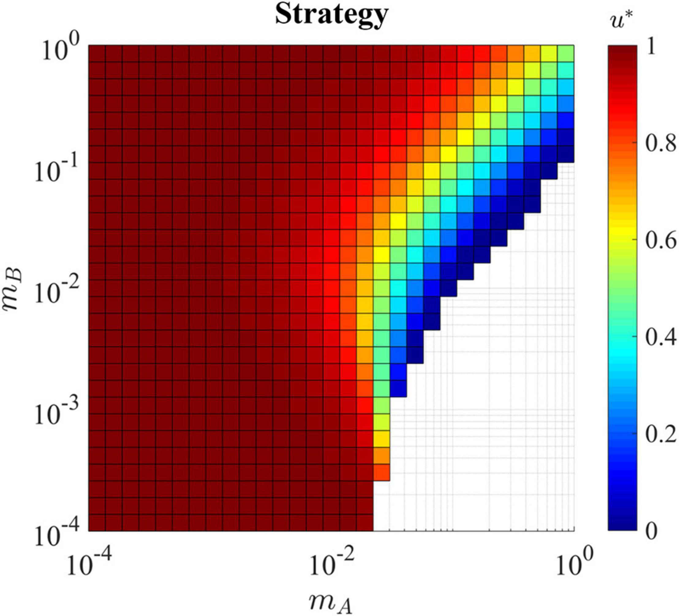
Figure 5. Evolutionary stable strategy in the presence of a hard sink for all combinations of m_A and m_B. With both migration rates slow (bottom left corner) the ESS remains equal to one as the exposure to the sink habitat is minimal. This is the same for the upper left corner where cells migrate at a slow rate out of habitat A and quickly migrate back, again minimizing the exposure to the sink habitat. In the lower right, the population can not survive as cell migrate quickly out of the source habitat and get ‘stuck’ in the hard sink, eventually dying before being able to return to the source where proliferation is possible. In the upper right corner where cells are migrating back and forth between the habitats quickly, the exposure to the sink habitat pulls the ESS u* away from 1 and toward the ESS of the sink habitat which is 0.

In the absence of migration from the sink habitat to the source, the hard sink acts like the black hole sink with the exception that during the transient dynamic to extinction, there can still be a sizable population in the sink habitat. Such transients are difficult to detect from histologies of biopsy samples, though indirectly one may be able to estimate birth and death rates of cancer cells from immunohistochemical stains such as Ki67 (a proliferation marker) and CC3 (an apoptosis marker of cell death) (Johnson et al., 2019).

When there is migration from the sink back to the source, then the eco-evolutionary prospects of the source habitat and tumor change dramatically. This becomes of interest as cancer cell movement from necrotic regions (micro-scale or large scale) or regions of hypoxia is likely within tumor microenvironments, especially when cancer cells remain relatively stationary while the habitats themselves form and shift in space.

Of most interest is when the migration rates m_A and m_B are such that the source population supports a population in the sink habitat. Under these migration rates, the ESS is a compromise between u^∗ = 0 and u^∗ = 1. A generalist species evolves that sacrifices carrying capacity in the source habitat for survivorship in the sink. In this way, the presence of a hard sink habitat pulls the ESS of the entire population, including those cells in the source habitat, away from the optimal strategy of the source habitat. Survival and reseeding from the sink becomes ecologically and evolutionarily consequential.

For example, Figure 6 shows how the adaptive landscape, cancer strategy value, and habitat-specific population sizes change over time for m_A = m_B = 10⁻¹. When the source habitat starts out relatively full and the sink habitat relatively empty, all cells have a strategy maximizing fitness in the source habitat, the adaptive landscape shows that decreasing the strategy value will increase overall fitness, G. The cancer cells’ strategy climbs the adaptive landscape until the slope of the landscape is zero (∂⁡G/∂⁡u = 0) and the population sizes equilibrates so that fitness is 0 (G=0). The ESS at this stable point is u^∗ = 0.5358, and the distribution of individuals between the two habitats is $N_A^{*}=63.18$ and $N_B^{*}=58.57$.

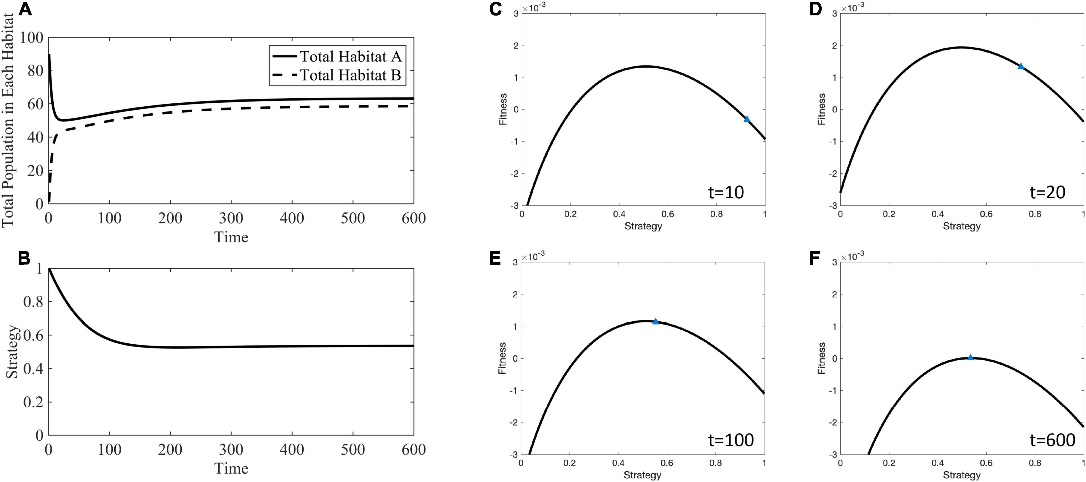
Figure 6. Ecological and evolutionary dynamics in the presence of hard sink where m_A = m_B = 10⁻¹. (A) Population dynamics of habitat A and B showing the quick migration out of the initially large source population to fill the sink habitat followed by dynamics toward the stable population densities. (B) The strategy value over time decreases away from 1 to a generalist strategy between 0 and 1. (C) The adaptive landscape at the initial conditions, where the source habitat is relatively full, the sink habitat is relatively empty, and all cells have a strategy maximizing fitness in the source habitat shows that fitness could be greatly increased by decreasing the strategy value and climbing the adaptive landscape. (D–F) As time progresses the strategy value climbs to an ESS of u^∗ = 0.5358. Supplementary Movie 1 provides a movie of the panels presented in (C–F).

This generalist strategy of u^∗ = 0.5358 allows for a total population size of N^∗ = 121.75 that is greater than the maximum population that can be sustained by the source habitat alone, 100. For all combinations of m_A≈m_B where both are greater than ≈10⁻², the total ESS population size is greater than 100, reaching a maximum possible N^* of 124.1 (Figure 7). With a sufficiently low d_B(v), the sink habitat can even harbor more individuals than the source habitat. For these reasons, the sink habitat can influence the ESS by selecting for a population wide u* < 1. This evolution allows the sink habitat to become a large reservoir of cells that can repopulate the source habitat following perturbations such as therapy. Population size alone cannot be used to infer which microhabitats in tumors are sources and hard sinks.

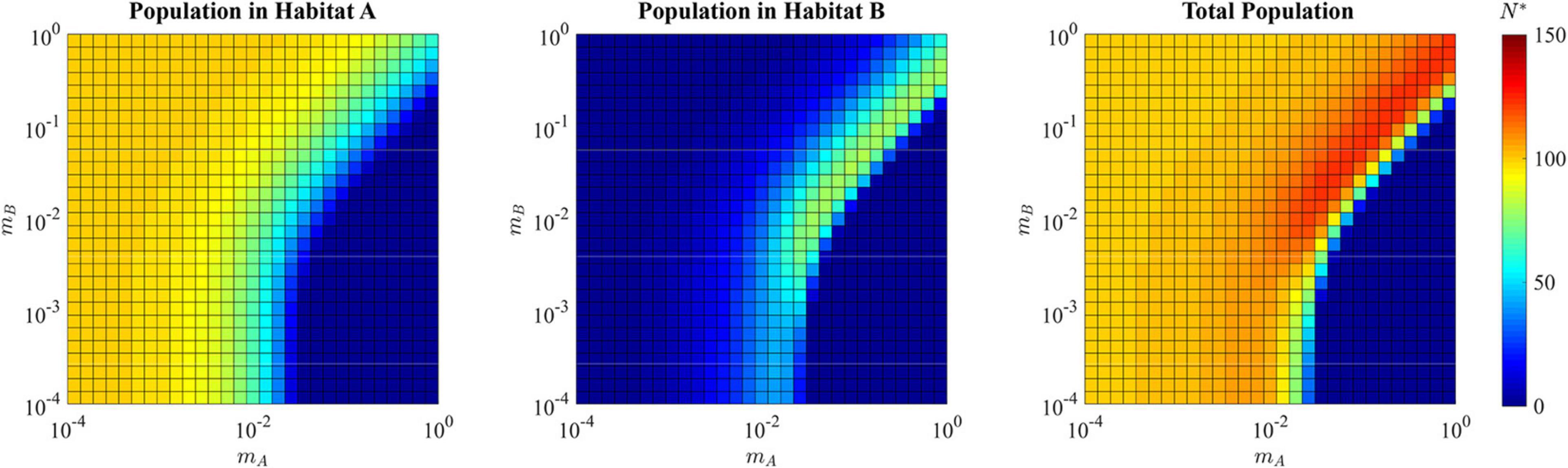
Figure 7. ESS population density of habitat A, habitat B, and the total combined population in the presence of a hard sink. The population is specialized to habitat A when the migration rate m_A is relatively low (lower left quadrant and upper left quadrant of each panel) reaching the carrying capacity of habitat A with relatively low density in habitat B. When the migration out of the source habitat A is fast and there is low migration back from the sink (lower right quadrant), the population declines to extinction. When there is a balance of migration rates (upper right quadrant), a generalist strategy allows for cells in both habitat A and habitat B, resulting in a total ESS population greater than would be available with only the source sink.

Soft Sink

In a soft sink, both habitats can support a population independently, allowing for positive per capita growth rates in each habitat when population sizes are small. This creates an opportunity not available in black hole or hard sinks for the ESS to contain two species when migration rates are relatively low. For example, Figure 8 shows the adaptive landscape and evolutionary dynamics over time for m_A = m_B = 10⁻³. Under the initial conditions, where habitat A is relatively full, habitat B relatively empty, and all cells have a strategy maximizing fitness in habitat A, the adaptive landscape shows that decreasing the strategy value will increase fitness. Interestingly, the convergent stable point is at a minimum of the landscape (∂²⁡G/∂⁡u² > 0), and the cancer cells should speciate, creating two distinct populations or “species” each with its own unique strategy. These species climb their respective peaks of the adaptive landscape to reach an ESS with two species.

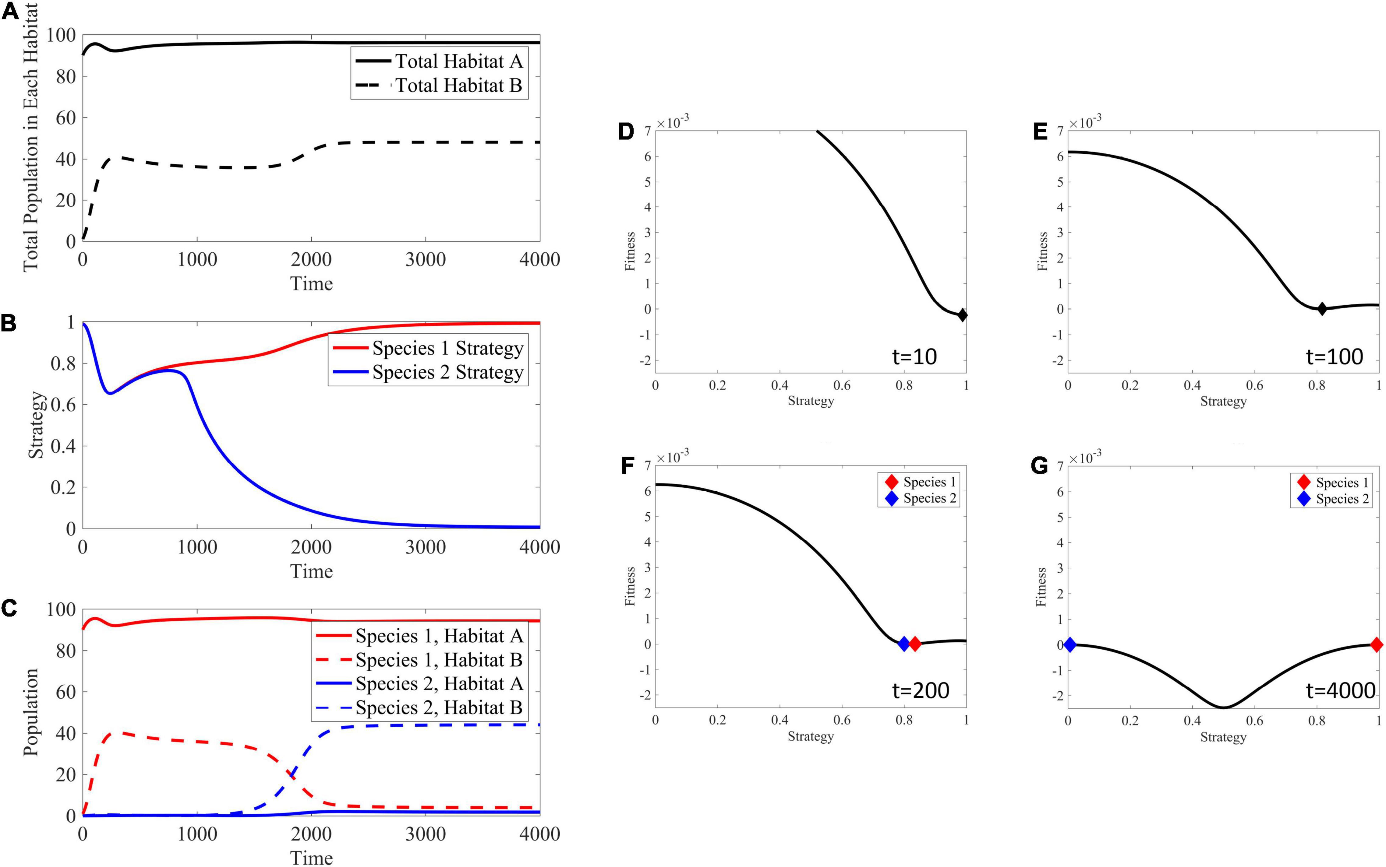
Figure 8. Ecological and evolutionary dynamics in the presence of soft sink where m_A = m_B = 10⁻³. (A) Population dynamics of habitat A and B showing habitat B filling up with migrant cells from the source habitat A, then both cell populations maximizing their respective carrying capacities after speciation. (B) The strategy value over time, showing a speciation event at around time 1000. These dynamics are seen in the panels (D–G) with respect to the underlying adaptive landscape. (C) The population densities broken down between both species and habitat. Species 1 is the only species filling both habitats before the speciation event. Afterwords, habitat B is filled with species 2 having a strategy equal to 0 maximizing fitness in this habitat, while habitat A remains filled with species 1. (D) The adaptive landscape at the initial conditions, where the source habitat is relatively full, the sink habitat is relatively empty, and all cells have a strategy maximizing fitness in the source habitat shows that fitness could be greatly increased by decreasing the strategy value and climbing the adaptive landscape. (E) The population evolves to a minimum in the adaptive landscape. (F,G) Speciation occurs and the individual species climb their respective peaks. Supplementary Movie 2 provides a movie of the panels presented in (D–G).

Each species becomes a specialist on their respective habitat. In this way, species 1 has a strategy of u^∗≈1 that maximizes carrying capacity in habitat A, while species 2 has a strategy of u^∗≈0 that maximizes carrying capacity in habitat B (bottom left corner of Figure 9). In cancer, this likely explains some of the heterogeneity in cancer cell types (Lloyd et al., 2016), and is most likely to promote diversity when habitats are relatively large and contiguous, thus reducing migration rates between them. In line with this, secondary tumors in different tissue types from the primary tumor will evolve cancer cells with quite distinctive phenotypes appropriate to the specific tissue type (Klein et al., 2002; Quinn et al., 2021). Such divergences have also been seen in 3-D cancer cell culture experiments (Ruud et al., 2020).

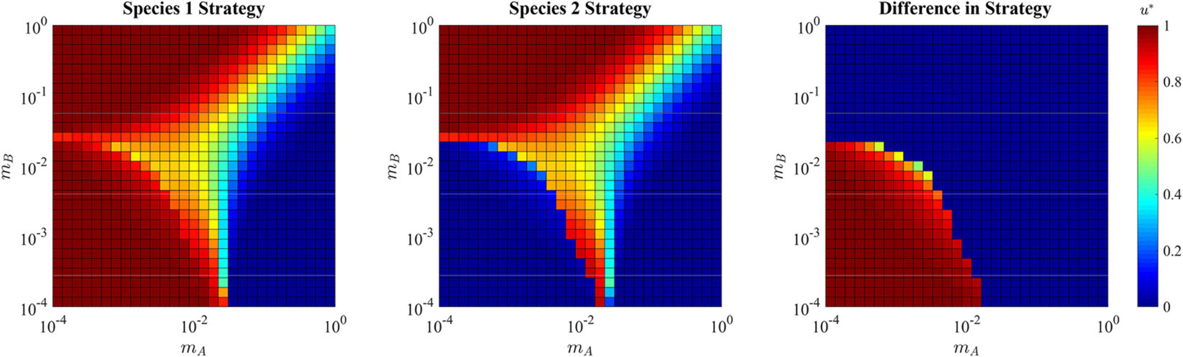
Figure 9. ESS in the presence of a soft sink. Due to the possibility of speciation, the strategy for both species 1 and species 2 are shown independently in the first two panels, and the differences between them is shown in the right panel. Where the population is specialized to habitat A (upper left quadrant) the single species ESS converges on u^∗ = 1. Where the population is specialized to habitat B (lower right quadrant) the single species ESS converges on u^∗ = 0. Where the population takes a single generalist approach (upper right quadrant) the ESS compromises and converges to a strategy between 0 and 1. Where the population speciates (lower left quadrant), each species converges to strategy that maximizes fitness in their respective habitats: u^∗ = 0 and u^∗ = 1.

When migration rates are relatively high for both m_A and m_B, the rapid movement of cells between habitats selects for a single generalist species (upper right corner of Figure 9). Interestingly, when m_A and m_Bare at opposite extremes (consider the upper left corners and lower right corners of Figure 9) the ESS tends to specialize on the habitat with high immigration and low emigration. For example, the upper left corner has high immigration into habitat A from habitat B, and low emigration from habitat A to habitat B. Here we see the ESS selects for u^∗ = 1, which is the optimal strategy for habitat A. The same is true, but opposite for the lower right corner.

The migration rates favoring a single generalist, single specialist, and speciation to two coexisting specialist species are shown in Figure 10.

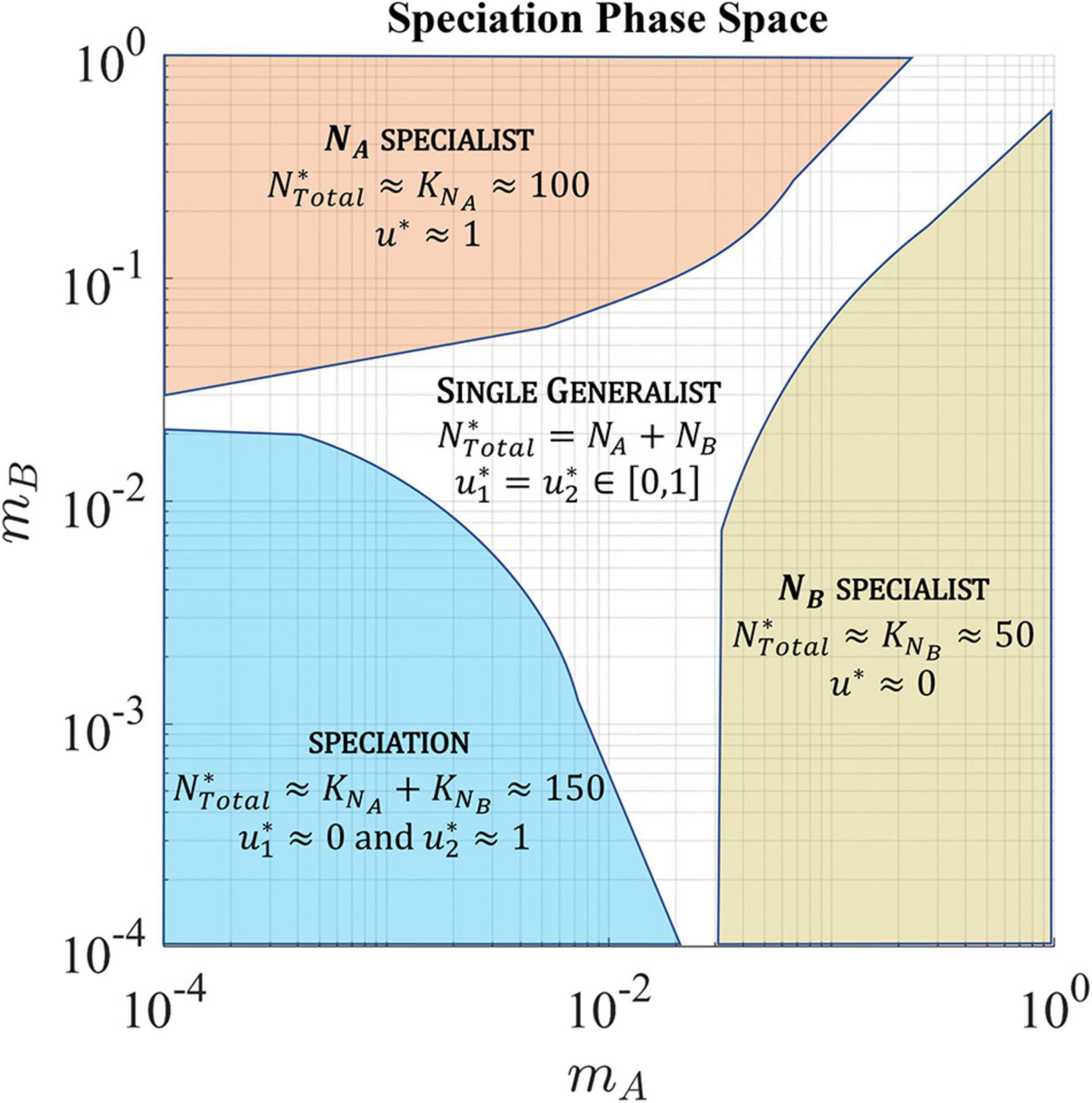
Figure 10. In a soft sink, migration rates, m_A and m_B, determine whether the ESS has a single generalist species, single specialist species, or speciation resulting in the coexistence of two specialist species. The population is specialized to habitat A (upper left quadrant) when the rate of cell migration out of habitat A is low and the rate of cell migration back into habitat A is high. Alternatively, the population is specialized to habitat B (lower right quadrant) when the rate of cell migration out of habitat B is low and the rate of cell migration back into habitat B is high. When the migration between both habitats in low, the population speciates with each species specializing on one habitat. In the other regions, the ESS converges to a single generalist species with a strategy that represents a compromise between the two habitats.

For the adaptive landscape example shown in Figure 8 where m_A = m_B = 10⁻³, the total ESS population is N^∗ = 144.2, well above the carrying capacity of the source habitat alone (Figure 11). In the single specialist regions, the total population is near or a little above the carrying capacity of the habitat to which the species is specialized. The region where a single generalist strategy is the ESS, like that in the hard sink, can also sustain total populations greater than each of the habitats individually.

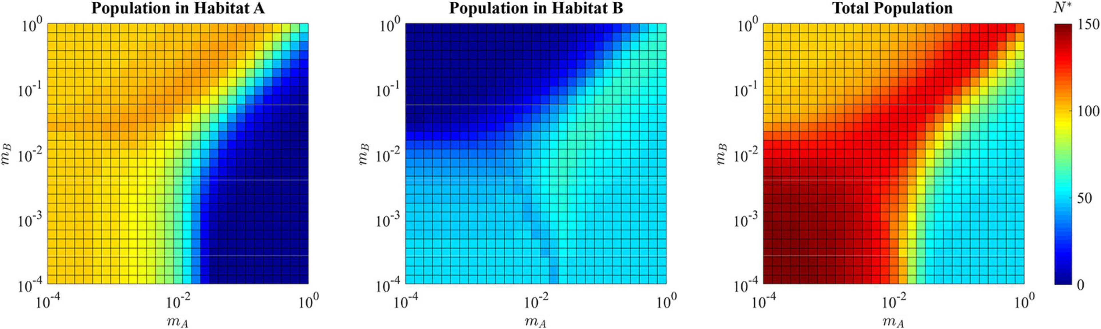
Figure 11. ESS population density of habitat A, habitat B, and the total combined population in the presence of a soft sink. Where the population is specialized to habitat A (upper left quadrant) the ESS population density reaches the carrying capacity of habitat A, with relatively low density in habitat B. Where the population is specialized to habitat B (lower right quadrant) the ESS population density reaches the carrying capacity of habitat B, with relatively low density in habitat A. Where the population evolves a generalist strategy (upper right quadrant) the ESS population can exceed the maximum carrying capacity provided in the source habitat, with substantial numbers of cancer cells in both habitat A and habitat B. Where the population speciates (lower left quadrant), each species can nearly reach its maximal carrying capacity within its preferred habitat, allowing the total ESS population to approach N^∗ = 150.

It is important to note that if each habitat can support individuals alone, the definition of the source and sink habitat are context dependent. There are indeed regions where the migration rates and populations in each habitat make habitat B the source where F_B > 0 and habitat A the sink where F_A < 0.

Consequences of Habitat-Dependent and Phenotype-Dependent Therapies

Witihin the context of a soft-sink, we set migration values to m_A = m_B = 10⁻³ so as to be in the speciation regime of the phase portrait, and analyze the eco-evolutionary dynamics of cancer cells under two types of therapy: habitat dependent and phenotype dependent. First, we consider habitat treatment under which all species in habitat A (the source habitat) are subject to the effects of therapy, regardless of their strategy. Species in habitat B are not directly affected by this treatment. In ecology, this is analogous to the application of pesticide to a portion of farmland. In cancer, it pertains to the pharmacokinetics of drug delivery through vasculature and the size of the tumor. The drug may only reach certain areas of the tumor at high concentrations (source habitats) but is unable to permeate other regions of the tumor (sink habitats), sheltering these cells from the effects of therapy.

To simulate habitat treatment, we simply eliminate 5% of the cells in habitat A at each time step in the simulation. This changes the source habitat into a sink habitat and vice versa. As such, cells in habitat A go extinct, while the cell populations in habitat B remain at their carrying capacity (Figures 12A,C). Since habitat A can no longer support any cells, species 1, which formerly specialized in habitat A, evolves toward a strategy of v = 0 converging on that of species 2 (Figure 12B). Even as species 1 evolves toward specializing on habitat B its population declines, potentially to extinction, as a consequence of species 2 already being a habitat B specialist. The ESS goes from two specialist species prior to therapy to a single specialist species following therapy. These changes can clearly be seen in the adaptive landscapes (Figures 12D–G). Before the application of therapy (Figure 12D), there exist two peaks on the adaptive landscape: one at v = 1, habitat A which species 1 occupies, and one at v=0, habitat B which species 2 occupies. However, once therapy is administered, the two peaks of the adaptive landscape change into a single peak at v=0, corresponding to being a habitat B specialist. Species 1 is initially entirely unfit for this habitat (Figure 12E), but eventually evolves (Figure 12F) and converges on the strategy at v=0 (Figure 12G).

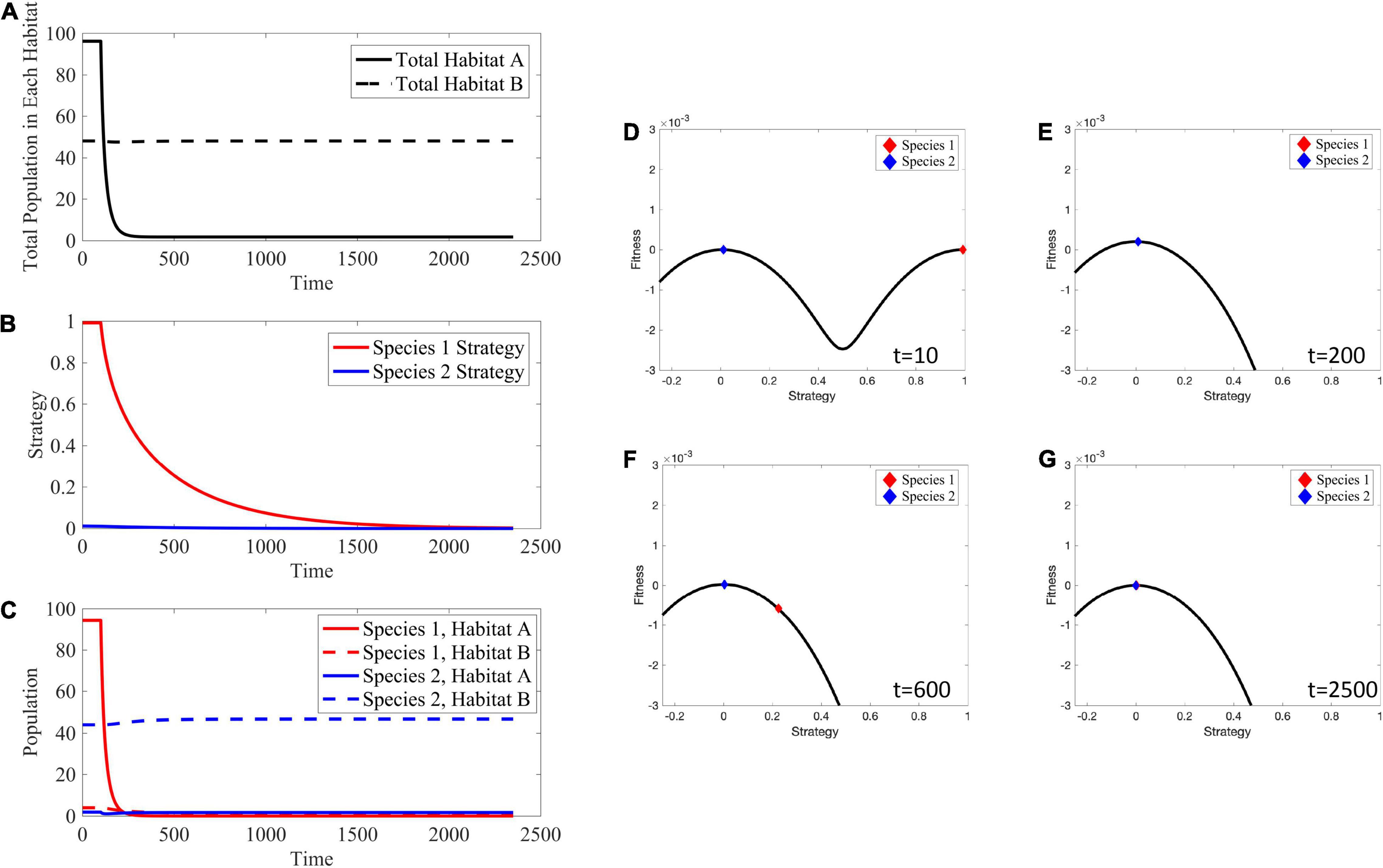
Figure 12. Effects of Habitat Treatment. Habitat A can no longer support any cells, and evolution drives species 1 to evolve toward v = 0 to persist in habitat B. (A) The total population in habitat A crashes to 0, while the total population in habitat B remains at its carrying capacity. (B) Since habitat A is no longer viable, species 1 evolves its strategy toward v = 0 in an attempt to remain extant in habitat B. (C) Species 1 crashes in habitat A after the application of treatment and is not able to evolve its strategy fast enough to persist in habitat B. There is little to no change in population density of species 2 in habitat B. (D–G) Depictions of the adaptive landscape over time. Before application of therapy, there are two peaks in the adaptive landscape, corresponding to the two viable habitats. After therapy is administered, the peak corresponding to habitat A vanishes and species 1 evolves toward the peak at v = 0. Supplementary Movie 3 provides a movie of the panels presented in (D–G).

Now, consider a phenotype-dependent therapy or targeted therapy whose efficacy depends on the species’ trait value, regardless of their habitat. In ecology, the targeted therapy may be analogous to fish harvesting by humans, with the species’ trait representing fish body size. In cancer, the targeted therapy (Herceptin) may target a specific protein (HER-2) in a cancer metabolic pathway. In both instances, one can imagine that the targeted therapy will not be effective at low values of the trait (a small fish or a cancer cell with a low expression of the target protein) but may be highly effective for high values of the trait.

We simulate targeted therapy by using a maximal efficacy of 5% at the cancer cell strategy at which the drug is maximally effective (v=1), with efficacy falling as v diverges from 1 (Figure 3). First, consider the overall dynamics in Figure 13A. We note that the total population (combined over both species) in habitat B remains remarkably constant for the entirety of the simulation. Because most of the individuals in habitat B have a strategy value less effected by the targeted therapy, cancer cells in habitat B suffer a smaller decline from therapy than those in habitat A. Because the targed therapy is most effective against cancer cells specialized on habitat A, the population in A drops dramatically immediately after therapy is administered. At least initially, this therapy that targets a cancer phenotype v=1has a similar effect as the habitat-dependent therapy. But, in time, the effect is dramatically different. Species 1, whether residing in habitats A or B, can evolve resistance by having a lower strategy value that also has the additional benefit of making species 1 more of a generalist.

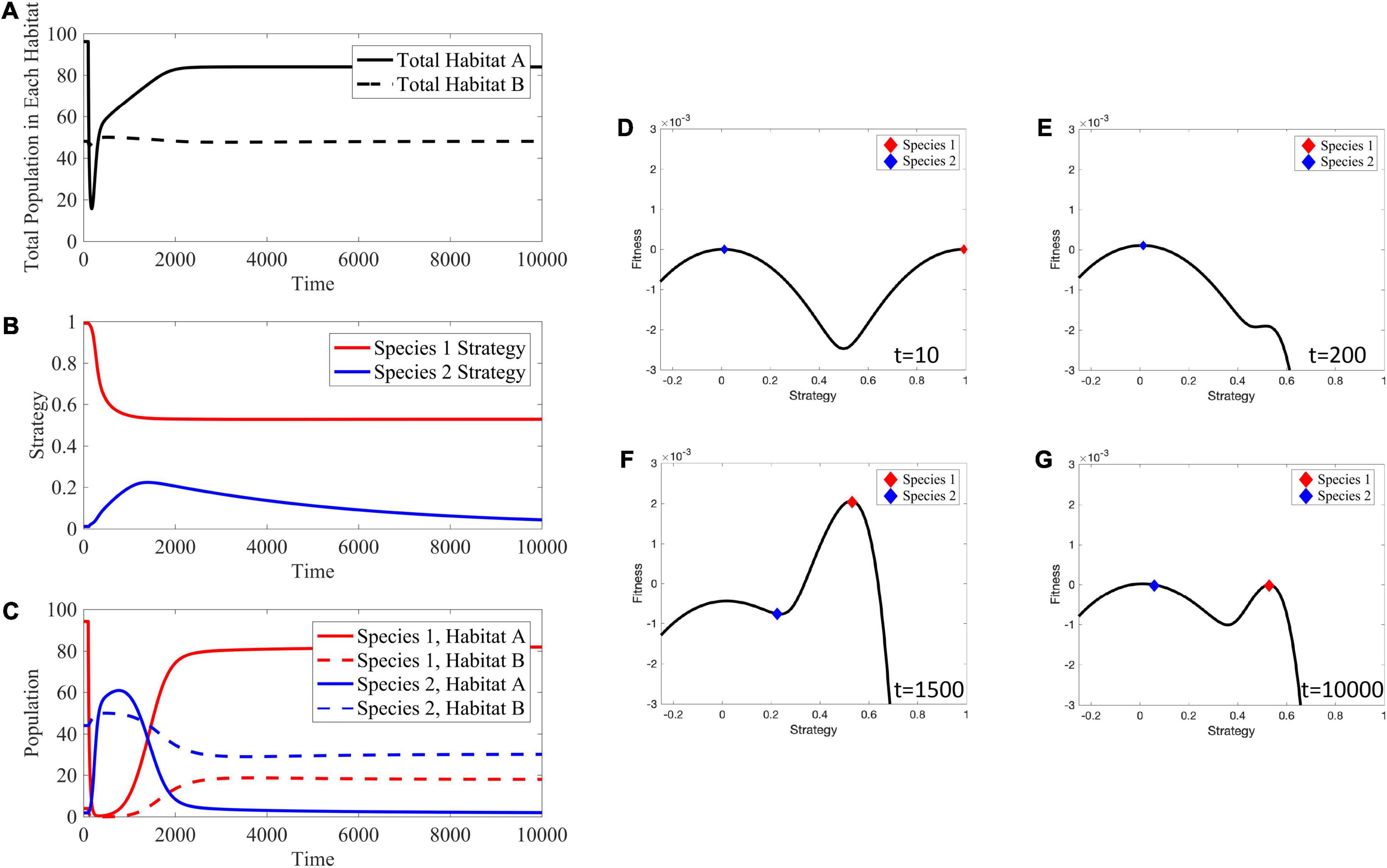
Figure 13. Effects of Targeted Therapy. (A) The total population in habitat A drastically declines immediately after administration of therapy, but gradually recovers as cells evolve viable trait values. The total population in habitat B stays near its carrying capacity. (B) Species 1 evolves a lower strategy to reduce impact of therapy. Species 2 initially evolves a higher strategy in an attempt to occupy the empty niche in habitat A. Once species 1 becomes viable in habitat A, species 2 evolves its strategy back down to near v = 0. (C) Transient dynamics: species 1′s population crashes and species 2 attempts to occupy the empty niche in habitat A. Long-term dynamics: species 1 evolves a lower strategy, allowing it to outcompete species 2 in habitat A and allowing species 1 to persist in habitat B at a lower level than species 2. (D–G) Depictions of the adaptive landscape over time. Before application of therapy, there are two peaks in the adaptive landscape, corresponding to the two viable habitats. After therapy is administered, the peak corresponding to habitat A shifts toward the one for habitat B; species 1 evolves toward this shifted peak. Supplementary Movie 4 provides a movie of the panels presented in (D–G).

Once species 1 evolves a lower strategy, evolutionary rescue is possible and population size recovers. However, note this lower strategy reduces the maximal carrying capacity in habitat A, leading to a lower population equilibrium than prior to treatment. Now, consider species-specific dynamics (Figures 13B,C) in which species 1 rapidly declines following therapy. Initially this leaves an open niche in habitat A to which species 2 evolves a higher strategy value. Thus, simultaneously, the strategies of both species 1 and species 2 begin to converge on more generalist phenotypes – species 1 as a form of therapy resistance and species 2 to take advantage of a depopulated habitat A.

Eventually, species 1 evolves into a generalist that allows it to be therapy resistant and to repopulate habitat A though not at the same abundance as pre-treatment. As species 1 recovers, species 2 is again under selection to be a habitat B specialist. Interestingly, at the new post-treatment ESS, species 1′s generalist strategy allows it to have substantial population sizes in both habitats at the expense of species 2. Compared to the pre-treatment ESS, species 2 is still virtually absent from habitat A and resides in habitat B at a reduced population size. While the transient dynamics of the adaptive landscape (Figures 13D–G) are dramatic, both the pre- and post-treatment ESSs lead to adaptive landscapes with two peaks. Once therapy is administered, habitat A’s peak shifts closer to habitat B’s, capturing a trade-off between maximizing carrying capacity in the habitat and avoiding effects of treatment.

The source-sink dynamics led to a counterintuitive result where targeting the phenotype of species 1 actually resulted in an increased number of this cancer cell type as the cancer cells evolved toward a new post-treatment ESS. This result happens because of the strong selection for habitat specialists with or without therapy. If there was only a weak tradeoff between habitat specialists then the pre-treatment system could either have a single generalist species or two specialist species that are not so extreme in their traits values. If the former, then with therapy, the single generalist species would evolve further toward being a habitat B specialist. If the latter, then the habitat A specialist might evolve so far toward the habitat B specialist or vice-versa that one type would go extinct leaving just a single generalist cancer cell type.

Discussion

Here, we investigate a relatively unrecognized dynamic in intratumoral evolution – the role of cell migration. Movement of individual cells can have population effects by coupling source-sink habitats, which we show can have profound consequences for tumor biology and treatment. Ongoing intratumoral evolution is frequently described as “branching clonal evolution.” That is, cancer cells are subject to genetic mutations and, when a rare mutation results in increased fitness, this new molecular clone expands into an observable population (Greaves and Maley, 2012). However, branching clonal evolution neglects the striking spatial heterogeneity in local environmental conditions, governed primarily by changes in blood perfusion, that are characteristically observed in cancers at macroscopic and microscopic levels. Thus, the selection forces within a tumor will vary considerably. Physically adjacent microscopic regions of a tumor can have dramatically different environmental conditions (Losic et al., 2020).

In contrast to this conventional “mutation-selection” sequence, we propose intratumoral evolution is primarily driven by spatial and temporal variations in environmental conditions. That is, cancer cells in regions of hypoxia and acidosis evolve different phenotypic properties than, for example, those in physiologic environments that may also contain more “predatory” immune cells. This generates frequency- and density-dependent selection within and between tumor microenvironments (Bozic et al., 2012; Soman et al., 2012) produce local cancer cell phenotypes and corresponding genotypes most suited to particular microenvironments – either as generalist or specialist cancer cell types. Thus, mutations that encode phenotypic adaptations suitable for the local environment will become frequent in the extant population. These genetic changes are consequences of evolution by natural selection, not the cause (Vincent and Brown, 1988).

Furthermore, a cancer biology paradigm that is difficult to reconcile with evolutionary dynamics is the stem cell hypothesis which posits self-replicating stem cells (Walcher et al., 2020) within a specific niche (Borovski et al., 2011; Oskarsson et al., 2014) give rise to phenotypically variable and non-replicating cells that populate the remainder of the tumor. Evolutionarily, the production of non-replicating daughter cells would be extremely wasteful of scarce resources and likely be subject to negative selection. However, these observed stem cell dynamics could arise from the migration of proliferative and phenotypically distinct cancer cells from source habitats to sink habitats where they adopt a different phenotype and are much less proliferative.

When migration occurs between a source and sink habitat, we demonstrate that, even when the sink habitat cannot maintain a long-term population (e.g., hard sink habitat), it can act as a reservoir of cells that migrate from the source habitat thus maximizing the global population. Furthermore, a harsh sink environment may promote epigenetic modifications (e.g., increased HIF1a expression resulting in upregulation of xenobiotic pathways (Vorrink and Domann, 2014)) that promote resistance to treatment. Thus, the sink habitat may become a source for cells that are also more resistant to subsequent cycles of treatment (Lavi et al., 2013).

In contrast, a soft sink habitat can maintain a small, self-reproducing population. Here, migration from the adjacent source habitat can increase the population of the sink habitat. However, unlike a black hole or hard sink habitat, cells that migrate into a soft sink habitat may proliferate. This is a critical distinction, because proliferation of the migrant cells in the sink habitat is determined by their fitness relative to that of competing native cells. Thus, although the migrant cells are the result of evolutionary selection in the source habitat, their proliferation in the sink habitat is governed by phenotypic adaptation to conditions in the sink habitat. These dynamics can promote “speciation” so that cancer cells even in adjacent tumor regions can have significantly different molecular properties.

Thus, migration of cancer cells between source and sink habitats can produce the clinically observed regional variations in the molecular properties of cancer cells as an alternative to the branching clonal evolution paradigm. Both the spatial variations in the molecular properties of cancer cells in the same tumor at microscopic and macroscopic scales (Gerlinger et al., 2012; Greaves and Maley, 2012; Gerashchenko et al., 2013; Losic et al., 2020) and cancer cell migration (Yamaguchi et al., 2005; Chung et al., 2010; Huang et al., 2011) have been extensively investigated. Yet, to date, no experiments have directly tested the source-sink dynamics described here. Microfluidic co-culture systems may provide an opportunity. There could be adjacent chambers with high (source) and low (soft or hard sink, depending) nutrient availabilities. Hydrogel stiffness could be used to vary migration rates into and out of chambers. Fluorescent labeling could allow for measures of migration, population dynamics, and phenotypic and genotypic changes over time both within and between chambers (Soman et al., 2012; Mi et al., 2016).

We note coupled source-sink habitats may additionally have clinical significance by promoting evolution of resistance following treatment. Thus, while therapy is successful in the source habitat due to increased drug delivery in the case of systemic therapy or improved oxygenation that increases the efficacy of radiation therapy, the source-sink dynamics could reverse after therapy as the surviving cells in the sink habitat become a source, allowing reverse migration and recolonization of the hitherto superior habitat (“rescue effect” in ecology, (Gotelli, 1991)). Adding therapy to the microfluidic co-culture experimental system could address these results.

Conclusion

In conclusion, the ecological and evolutionary dynamics produced by source-sink habitats may provide an underlying explanation to observed spatial variations in genetic and phenotypic properties of cancer cells, an eco-evolutionary foundation for the stem cell paradigm, and suggest critical issues in designing chemotherapeutic and targeted treatment strategies.

Data Availability Statement

The original contributions presented in the study are included in the article/Supplementary Material, further inquiries can be directed to the corresponding author/s.

Author Contributions

RAG, JSB, and JJC developed the hypothesis. JJC, AB, and JSB developed and analyzed the mathematical models. RAG, RJG, JJC, AB, and JSB wrote and edited the article. All authors contributed to the article and approved the submitted version.

Funding

This work was supported by the James S. McDonnell Foundation grant, “Cancer therapy: Perturbing a complex adaptive system,” grants from the Jacobson Foundation, NIH/National Cancer Institute (NCI) R01CA170595, Application of Evolutionary Principles to Maintain Cancer Control (PQ21), and NIH/NCI U54CA143970-05 (Physical Science Oncology Network (PSON)) “Cancer as a complex adaptive system”. This work has also been supported in part by the European Union’s Horizon 2020 Research and Innovation Program under the Marie Skłodowska-Curie Grant Agreement No. 690817 and the National Science Foundation Graduate Research Fellowship Program under Grant No. 1746051.

Disclaimer

Any opinions, findings, and conclusions or recommendations expressed in this material are those of the author and do not necessarily reflect the views of the National Science Foundation.

Conflict of Interest

The authors declare that the research was conducted in the absence of any commercial or financial relationships that could be construed as a potential conflict of interest.

The handling editor declared a past collaboration with one of the authors, JB.

Supplementary Material

The Supplementary Material for this article can be found online at: https://www.frontiersin.org/articles/10.3389/fevo.2021.676071/full#supplementary-material

References

Archetti, M. (2013). Evolutionary game theory of growth factor production: implications for tumour heterogeneity and resistance to therapies. Br. J. Cancer. 109, 1056–1062. doi: 10.1038/bjc.2013.336
Borovski, T., De Sousa, E. M. F., Vermeulen, L., and Medema, J. P. (2011). Cancer stem cell niche: the place to be. Cancer Res. 71, 634–639.
Boughton, D. A. (1999). Source-sink dynamics in a temporally, heterogeneous environment. Ecology 80, 2727–2739.
Bozic, I., Allen, B., and Nowak, M. A. (2012). Dynamics of targeted cancer therapy. Trends Mol. Med. 18, 311–316.
Brown, J. S., and Pavlovic, N. (1992). Evolution in heterogeneous environments: effects of migration on habitat specialization. Evol. Ecol. 6, 360–382. doi: 10.1007/bf02270698
Chung, S., Sudo, R., Vickerman, V., Zervantonakis, I. K., and Kamm, R. D. (2010). Microfluidic platforms for studies of angiogenesis, cell migration, and cell–cell interactions. Ann. Biomed. Eng. 38, 1164–1177. doi: 10.1007/s10439-010-9899-3
Cohen, Y. V. T., and Brown, J. S. (1999). A G-function approach to fitness minima, fitness maxima, evolutionarily stable strategies and adaptive landscapes. Evol. Ecol. Res. 1, 923–942.
Cure, K., Thomas, L., Hobbs, J. A., Fairclough, D. V., and Kennington, W. J. (2017). Genomic signatures of local adaptation reveal source-sink dynamics in a high gene flow fish species. Sci. Rep. 7:8618.
Diffendorfer, J. E. (1998). Testing models of source-sink dynamics and balanced dispersal. Oikos 81, 417–433. doi: 10.2307/3546763
Dongre, A., and Weinberg, R. A. (2019). New insights into the mechanisms of epithelial-mesenchymal transition and implications for cancer. Nat. Rev. Mol. Cell Biol. 20, 69–84. doi: 10.1038/s41580-018-0080-4
Fisher, R., Larkin, J., and Swanton, C. (2012). Inter and intratumour heterogeneity: a barrier to individualized medical therapy in renal cell carcinoma? Front. Oncol. 2:49. doi: 10.3389/fonc.2012.00049
Fu, F., Nowak, M. A., and Bonhoeffer, S. (2015). Spatial heterogeneity in drug concentrations can facilitate the emergence of resistance to cancer therapy. PLoS Comput. Biol. 11:e1004142. doi: 10.1371/journal.pcbi.1004142
Gerashchenko, T. S., Denisov, E. V., Litviakov, N. V., Zavyalova, M. V., Vtorushin, S. V., Tsyganov, M. M., et al. (2013). Intratumor heterogeneity: nature and biological significance. Biochemistry (Mosc) 78, 1201–1215. doi: 10.1134/s0006297913110011
Geritz, S. A. H., Kisdi, E’., Mesze’NA, G., and Metz, J. A. J. (1998). Evolutionarily singular strategies and the adaptive growth and branching of the evolutionary tree. Evol. Ecol. 12, 35–57. doi: 10.1023/A:1006554906681
Gerlinger, M., Rowan, A. J., Horswell, S., Math, M., Larkin, J., Endesfelder, D., et al. (2012). Intratumor heterogeneity and branched evolution revealed by multiregion sequencing. N. Engl. J. Med. 366, 883–892. doi: 10.1056/NEJMoa1113205
Gotelli, N. J. (1991). Metapopulation models: the rescue effect, the propagule rain, and the core-satellite hypothesis. Am. Nat. 138, 768–776. doi: 10.1086/285249
Gravel, D., Guichard, F., Loreau, M., and Mouquet, N. (2010). Source and sink dynamics in meta-ecosystems. Ecology. 91, 2172–2184. doi: 10.1890/09-0843.1
Hinohara, K., and Polyak, K. (2019). Intratumoral heterogeneity: more than just mutations. Trends Cell Biol. 29, 569–579. doi: 10.1016/j.tcb.2019.03.003
Holt, R. (1985). Population-dynamics in 2-patch environments - some anomalous consequences of an optimal habitat distribution. Theor. Popul. Biol. 28, 181–208. doi: 10.1016/0040-5809(85)90027-9
Holt, R. D., and Gomulkiewicz, R. (1997). How does immigration influence local adaptation? A reexamination of a familiar paradigm. Am. Nat. 149, 563–572. doi: 10.1086/286005
Holt, R. D., Barfield, M., and Gomulkiewicz, R. (2004). Temporal variation can facilitate niche evolution in harsh sink environments. Am. Nat. 164, 187–200. doi: 10.2307/3473438
Huang, Y., Agrawal, B., Sun, D., Kuo, J. S., and Williams, J. C. (2011). Microfluidics-based devices: new tools for studying cancer and cancer stem cell migration. Biomicrofluidics 5:013412. doi: 10.1063/1.3555195
Jardim-Perassi, B. V., Huang, S., Dominguez-Viqueira, W., Poleszczuk, J., Budzevich, M. M., Abdalah, M. A., et al. (2019). Multiparametric MRI and coregistered histology identify tumor habitats in breast cancer mouse models. Cancer Res. 79, 3952–3964. doi: 10.1158/0008-5472.can-19-0213
Johnson, D. M. (2004). Source-sink dynamics in a temporally, heterogeneous environment. Ecology 85, 2037–2045. doi: 10.1890/03-0508
Johnson, K. E., Howard, G., Mo, W., Strasser, M. K., Lima, E., Huang, S., et al. (2019). Cancer cell population growth kinetics at low densities deviate from the exponential growth model and suggest an Allee effect. PLoS Biol. 17:e3000399. doi: 10.1371/journal.pbio.3000399
Klein, C. A., Blankenstein, T. J., Schmidt-Kittler, O., Petronio, M., Polzer, B., Stoecklein, N. H., et al. (2002). Genetic heterogeneity of single disseminated tumour cells in minimal residual cancer. Lancet. 360, 683–689. doi: 10.1016/s0140-6736(02)09838-0
Lavi, O., Greene, J. M., Levy, D., and Gottesman, M. M. (2013). The role of cell density and intratumoral heterogeneity in multidrug resistance. Cancer Res. 73, 7168–7175. doi: 10.1158/0008-5472.can-13-1768
Li, F., Tiede, B., Massague, J., and Kang, Y. (2007). Beyond tumorigenesis: cancer stem cells in metastasis. Cell Res. 17, 3–14. doi: 10.1038/sj.cr.7310118
Lloyd, M. C., Cunningham, J. J., Bui, M. M., Gillies, R. J., Brown, J. S., and Gatenby, R. A. (2016). Darwinian dynamics of intratumoral heterogeneity: not solely random mutations but also variable environmental selection forces. Cancer Res. 76, 3136–3144. doi: 10.1158/0008-5472.can-15-2962
Losic, B., Craig, A. J., Villacorta-Martin, C., Martins-Filho, S. N., Akers, N., Chen, X., et al. (2020). Intratumoral heterogeneity and clonal evolution in liver cancer. Nat Commun. 11:291.
Mi, S., Du, Z., Xu, Y., Wu, Z., Qian, X., Zhang, M., et al. (2016). Microfluidic co-culture system for cancer migratory analysis and anti-metastatic drugs screening. Sci. Rep. 6, 1–11.
Moreno-Gamez, S., Hill, A. L., Rosenbloom, D. I., Petrov, D. A., Nowak, M. A., and Pennings, P. S. (2015). Imperfect drug penetration leads to spatial monotherapy and rapid evolution of multidrug resistance. Proc. Natl. Acad. Sci.U.S.A. 112, E2874–E2883.
Morris, D. W. (1991). On the evolutionary stability of dispersal to sink habitats. Am. Nat. 137, 907–911. doi: 10.1086/285200
Oskarsson, T., Batlle, E., and Massague, J. (2014). Metastatic stem cells: sources, niches, and vital pathways. Cell Stem Cell. 14, 306–321. doi: 10.1016/j.stem.2014.02.002
Paul, C. D., Mistriotis, P., and Konstantopoulos, K. (2017). Cancer cell motility: lessons from migration in confined spaces. Nat. Rev. Cancer 17, 131–140. doi: 10.1038/nrc.2016.123
Perez-Velazquez, J., and Rejniak, K. A. (2020). Drug-induced resistance in micrometastases: analysis of spatio-temporal cell lineages. Front. Physiol. 11:319. doi: 10.3389/fphys.2020.00319
Polacheck, W. J., Zervantonakis, I. K., and Kamm, R. D. (2013). Tumor cell migration in complex microenvironments. Cell Mol. Life Sci. 70, 1335–1356. doi: 10.1007/s00018-012-1115-1
Pulliam, H. R. (1988). Sources, sinks, and population regulation. Am. Nat. 132, 652–661. doi: 10.1086/284880
Quinn, J. J., Jones, M. G., Okimoto, R. A., Nanjo, S., Chan, M. M., Yosef, N., et al. (2021). Single-cell lineages reveal the rates, routes, and drivers of metastasis in cancer xenografts. Science 371, eabc1944. doi: 10.1126/science.abc1944
Ruud, K. F., Hiscox, W. C., Yu, I., Chen, R. K., and Li, W. (2020). Distinct phenotypes of cancer cells on tissue matrix gel. Breast Cancer Res. 22:82.
Schmidt, K. A., Earnhardt, J. M., Brown, J. S., and Holt, R. D. (2000). Habitat selection under temporal heterogeneity: exorcizing the ghost of competition past. Ecology. 81, 2622–2630. doi: 10.1890/0012-9658(2000)081[2622:hsuthe]2.0.co;2
Scott, J., and Marusyk, A. (2017). Somatic clonal evolution: a selection-centric perspective. Biochim. Biophys. Acta 1867, 139–150. doi: 10.1016/j.bbcan.2017.01.006
Soman, P., Kelber, J. A., Lee, J. W., Wright, T. N., Vecchio, K. S., Klemke, R. L., et al. (2012). Cancer cell migration within 3D layer-by-layer microfabricated photocrosslinked PEG scaffolds with tunable stiffness. Biomaterials 33, 7064–7070. doi: 10.1016/j.biomaterials.2012.06.012
Staneva, R., El Marjou, F., Barbazan, J., Krndija, D., Richon, S., Clark, A. G., et al. (2019). Cancer cells in the tumor core exhibit spatially coordinated migration patterns. J. Cell Sci. 132: jcs220277.
Tarjuelo, R., Traba, J., Morales, M. B., and Morris, D. W. (2017). Isodars unveil asymmetric effects on habitat use caused by competition between two endangered species. Oikos 126, 73–81. doi: 10.1111/oik.03366
Te Boekhorst, V., Preziosi, L., and Friedl, P. (2016). Plasticity of cell migration in vivo and in silico. Annu. Rev. Cell Dev. Biol. 32, 491–526. doi: 10.1146/annurev-cellbio-111315-125201
Vincent, T. L., and Brown, J. (1988). The evolution of ESS theory. Ann. Rev. Ecol. Syst. 19, 423–443.
Vincent, T. L., and Brown, J. (2002). Evolutionarily stable strategies in multistage biological systems. Selection 2, 85–102. doi: 10.1556/select.2.2001.1-2.7
Vincent, T. L., and Brown, J. S. (2005). Evolutionary Game Theory, Natural Selection, and Darwinian Dynamics. Cambridge, NY: Cambridge University Press.
Vincent, T. L., Cohen, Y., and Brown, J. S. (1993). Evolution via strategy dynamics. Theor. Popul. Biol. 44, 149–176. doi: 10.1006/tpbi.1993.1023
Vorrink, S. U., and Domann, F. E. (2014). Regulatory crosstalk and interference between the xenobiotic and hypoxia sensing pathways at the AhR-ARNT-HIF1alpha signaling node. Chem. Biol. Interact. 218, 82–88. doi: 10.1016/j.cbi.2014.05.001
Walcher, L., Kistenmacher, A. K., Suo, H., Kitte, R., Dluczek, S., Strauss, A., et al. (2020). Cancer stem cells-origins and biomarkers: perspectives for targeted personalized therapies. Front. Immunol. 11:1280. doi: 10.3389/fimmu.2020.01280
Wang, H. F., Warrier, T., Farran, C. A., Zheng, Z. H., Xing, Q. R., Fullwood, M. J., et al. (2020). Defining essential enhancers for pluripotent stem cells using a features-oriented crispr-cas9 screen. Cell Rep. 33:108309. doi: 10.1016/j.celrep.2020.108309
Yamaguchi, H., Wyckoff, J., and Condeelis, J. (2005). Cell migration in tumors. Curr. Opin. Cell Biol. 17, 559–564. doi: 10.1016/j.ceb.2005.08.002
Keywords: cancer heterogeneity, cancer vascularity, branching clonal evolution, source-sink habitats, cancer ecology, cancer evolution
Citation: Cunningham JJ, Bukkuri A, Brown JS, Gillies RJ and Gatenby RA (2021) Coupled Source-Sink Habitats Produce Spatial and Temporal Variation of Cancer Cell Molecular Properties as an Alternative to Branched Clonal Evolution and Stem Cell Paradigms. Front. Ecol. Evol. 9:676071. doi: 10.3389/fevo.2021.676071
Received: 04 March 2021; Accepted: 28 June 2021;
Published: 20 July 2021.
Edited by:
Sarah R. Amend, Johns Hopkins Medicine, United StatesReviewed by:
Atsushi Niida, The University of Tokyo, JapanMichael Nicholson, University of Edinburgh, United Kingdom
Copyright © 2021 Cunningham, Bukkuri, Brown, Gillies and Gatenby. This is an open-access article distributed under the terms of the Creative Commons Attribution License (CC BY). The use, distribution or reproduction in other forums is permitted, provided the original author(s) and the copyright owner(s) are credited and that the original publication in this journal is cited, in accordance with accepted academic practice. No use, distribution or reproduction is permitted which does not comply with these terms.
*Correspondence: Robert A. Gatenby, Robert.gatenby@moffitt.org