
Abstract
Plant recognition has great potential in forestry research and management. A new method combined back propagation neural network and radial basis function neural network to identify tree species using a few features and samples. The process was carried out in three steps: image pretreatment, feature extraction, and leaf recognition. In the image pretreatment processing, an image segmentation method based on hue, saturation and value color space and connected component labeling was presented, which can obtain the complete leaf image without veins and background. The BP-RBF hybrid neural network was used to test the influence of shape and texture on species recognition. The recognition accuracy of different classifiers was used to compare classification performance. The accuracy of the BP-RBF hybrid neural network using nine dimensional features was 96.2%, highest among all the classifiers.
Introduction
Forest resources play an important role in the development of economies, societies and the environment (Yang and Kan 2020). However, in recent years, the natural environment has been severely damaged in many countries, resulting in the reduction of forest area and the extinction of many species. However, there is a new awareness of the importance of protecting plant species. A fundamental premise of plant protection is the accurate recognition and classification of plants (Gong and Cao 2014). On the one hand, recognition of plant species can help understand the forest ecosystem and forest economy (Nevalainen et al. 2017); on the other, it helps strengthen the management and protection of forest resources, and improve the public’s awareness of forest protection.
Plant recognition and classification based on image features is an important research focus in biodiversity informatics, and it is beneficial to explore the evolutionary rules and relationships of plants and establish a taxonomic database. The recognition of tree species is often difficult because of the existence of numerous species and the similarities among some species. The amount of information contained in leaves is considered and manifested in the colors, shapes, textures, veins and edges. Leaves are easy to collect and process with digital equipment. Based on the above characteristics, leaves are often used for species recognition (Rahman et al. 2019).
Information on species composition of an urban forest is essential for its management. However, this information is increasingly difficult to obtain due to limited taxonomic expertise of the urban managers. Traditional leaf recognition methods require a significant professional knowledge, and in its absence, may result in low efficiency. With the rapid development of computer technology, researchers are able to combine the image processing method, pattern recognition and machine learning technology with plant morphology to ascertain the automatic recognition of leaf images. Wu et al. (2007) extracted 12 digital morphological features on Flavia dataset (a widely used leaf dataset) and used the probabilistic neural network (PNN) to test the accuracy of their algorithm. The result was very similar to other systems (90%). Turkoglu et al. (2019) proposed that leaf feature extraction may be completed by dividing the leaf image into two or four parts. The accuracy of their method with the Flavia dataset was 99.1%. In their study, image processing based on feature extraction methods such as color, veins, Fourier descriptors (FD), and gray-level co-occurrence matrix (GLCM) were used. Tang (2020) used the grey cluster analysis method to establish a quantitative feature system of leaves, and used a probabilistic neural network for classification. The results were to evaluate model performance and the influence of core features of the model. The results showed that an accuracy of the GBDT-PNN model using 12 core features was 92.7%, and the accuracy with all 35 features was 93.5%.
Although there have been numerous advances on leaf classification based on machine learning, there are still some shortcomings. Few researchers have analyzed the influence of different features on recognition. Most studies have selected too many features, which faced challenges in practical application. In the process of leaf image pretreatment, the binary image obtained contains noise after image segmentation, usually caused by highlights on the leaf surface and dust particles scattered on the image acquisition device. Traditional denoising methods usually mistake noise-polluted leaf surface for background.
Given these problems, this study proposed an image segmentation method based on HSV color space and connected component labeling, which can completely extract leaves without petiole. The extracted image had a good denoising performance. In addition, shape and texture were extracted, and the leaf recognition performance of various machine learning methods was compared, and a BP-RBF hybrid neural network was newly established.
This system is a software solution for automatic recognition and classification of plant species. The scheme is divided into four main steps: (1) color space conversion of images; (2) image pretreatment; (3) leaf feature extraction; and (4) design of classifier and recognition. The basic flow of the leaf identification system is shown in Fig. 1.

Flow diagram of leaf recognition
Materials and methods
Sample preparation
In order to achieve the recognition and classification of species, the necessary preparation work is to establish a leaf database (Backes et al. 2009; Kumar et al. 2012). The research area was the Experimental Forest Farm of the Northeast Forestry University, with geographic coordinates 45°71′ − 45°72′ N, 126°62′ − 126°63′ E. The dataset comprised 366 images of leaves belonging to 15 common species in Northeast China. The scientific names and sample numbers are shown in Table 1.
Leaves with common shapes, complete fronds, spotless, and without pests were chosen, including petioles. Dust was removed from leaves; LEDs were used to illuminate leaves, and all leaf samples were photographed with a Nikon D850 digital camera. Leaf images of each species are shown in Fig. 2.

Samples of leaf images used for classification (The numbers correspond to the names in Table 1)
Image pretreatment
The RGB color space does not distinguish between brightness and color information and so the images are converted to HSV color space which has good linear scalability and is directly oriented to human visual perception (Perona and Malik 1990). Based on HSV images, the background was well separated, leaf contours were extracted and the noise was initially removed. The Otsu algorithm (Chang et al. 2018; Yu et al. 2019) was selected as the threshold segmentation method proposed by Otsu (1979). The basic principle is to find the best threshold to maximize the variance within or between clusters to accurately classify background and foreground content. However, the Otsu algorithm is very sensitive to noise, so noise should be eliminated using image smoothing algorithms.
Feature extraction
In the process of feature extraction, shape features (Wu et al. 2007; Wang et al. 2008) and texture features (Haralick 1973) are the two most commonly used recognition features.
Shape features
Shape is one of the most important features for characterizing a leaf because it can be perceived by humans (Wang et al. 2008). According to the extracted leaf contour, several geometric parameters (Wu et al. 2007) were calculated, including leaf area (S), the smallest rectangular area surrounding the leaf (S0), the perimeter of the leaf area (L), length (b) and width (a) of the minimum enclosing rectangle of the leaf, the coordinates (x0, y0) of the center of mass of the leaf, the coordinates (x, y) of the upper left corner of the rectangle, the length (X and Y) of the rectangle in the x and y directions, the maximum deflection angle (m) and the total number of groups (M) of the leaf profile. These geometric parameters were used to further calculate the following five shape features:
Rectangularity: the ratio of leaf area (S) to the smallest rectangle surrounding the leaf (S0)
Roundness: the similarity between leaf contour and circle.and circle
where, S is leaf area and L is the perimeter.
Aspect ratio: the ratio of length (b) to width (a) of the smallest enclosing rectangle
Deviation degree: the offset degree of the leaf centroid relative to the smallest enclosing rectangle
where, (x0, y0) is the coordinates of the center of mass of the leaf, (x, y) is the coordinates of the upper left corner of the rectangle, X and Y are the length of the rectangle in the x and y directions.
Sawtooth degree: the ratio of the maximum deflection angle (m) to the total number of leaf profiles (M)
Texture features
Texture features can be used to quantitatively describe the texture information. The secondary statistics obtained by the gray level co-occurrence matrix (Haralick 1973) reflects the texture features and is based on the relation between two neighboring pixels in a gray image. This study selected the following four features:
Contrast: It reflects the sharpness of the image and the depth of the texture.
where \(\delta (i,j) = \left| {i - j} \right|\) is the gray difference between neighboring pixels, \(P(i,j)\) is the gray value of the image.
Correlation: It indicates the gray level similarity in the row or column direction.
where \(\mu _{i}\), \(\mu _{j}\), \(\sigma _{i}\) and \(\sigma _{j}\) are the means and standard deviations of the rows and columns of the gray value \(P(i,j)\).
Energy: It is a measure of the stability degree of the grayscale change of the image texture.
Homogeneity: It represents the local uniformity of the image
In the above formulas, i and j are coordinates (row and column) of a pixel in the image. \(P(i,j)\) is the gray value of the pixel located at coordinates (i, j) in a leaf image.
Support vector machine
Support vector machine (SVM), originally developed by Vladimir Vapnik, is a powerful tool for solving nonlinear classification, function estimation, and density estimation problems (Zhang et al. 2018). SVM has a great advantage in solving the problems of small samples, and nonlinear and high-dimensional pattern recognition because the test error for the independent test set is smaller than other machine learning algorithms. Plant leaf recognition and classification is a complex classification problem. However, due to the limitation of leaf numbers, it is difficult to collect a large number of image samples for each kind of foliage plants, which is possible with the SVM classifier. Hence, this paper built a SVM classifier model. The main process is shown in Fig. 3.

Flow diagram of SVM classifier
SVM is based on the principle of risk minimization, which means that the empirical risk and confidence intervals are quite large. Therefore, the output of the model is the optimal solution (Nelson et al. 2008; Roy and Bhattacharya 2010; Tarjoman et al. 2012). The basic idea is to use a nonlinear mapping algorithm to convert the linearly inseparable samples of the low-dimensional input feature space into a high-dimensional feature space, making it linearly separable.
The optimal hyperplane can be obtained by solving the following quadratic optimization problem:
In the case of a particularly large number of features, this problem can be transformed into its dual problem:
where, \(\alpha = (\alpha _{1} , \cdots \cdots ,\alpha _{n} )\) is the Lagrange multiplier, \(w^{*}\) is the normal vector of the optimal hyperplane, and b1 is the offset of the optimal hyperplane. In the solution and analysis of this type of optimization problem, the Karush–Kuhn–Tucker (KKT) condition will play a very important role. In the second constraint formula, the solution must satisfy Eq. (16):
where, the samples of \(\alpha _{i} > 0\) are called support vectors.
The final classification function is as follows.
BP-RBF neural network
A neural network is a complex machine learning algorithm used for prediction analysis. It is trained with a set of inputs and outputs, and implicit relationships between inputs and outputs are extracted. The back propagation neural network (BPNN) is a type of multilayer forward neural network, which has strong data compression and fault tolerance abilities (Rumelhart et al. 1986). It is commonly used in the fields of pattern recognition, data classification and predictive analysis because of its good adaptability and robustness (Xu et al. 2018; Yang and Kan 2020).
The radial basis function neural network (RBFNN) has the ability to approximate functions with arbitrary precision. Based on the previous study using BPNN to identify plant leaves, BPNN and RBFNN are connected in series to form a BP-RBF hybrid neural network in this article. The network structure is shown in Fig. 4.

BP-RBF neural network structure
Results
Image pretreatment
The leaf RGB image was converted to HSV color space (Fig. 5). The optimal threshold obtained by the Otsu algorithm was used to convert the S component image into a binary image. Traditional denoising methods mainly include median and mean filtering and Gaussian low-pass filtering. None of the smoothing methods can completely remove background noise and leaf veins. There was still unremoved noise inside the leaves in Fig. 6b. For the purpose of eliminating noise, this research presented a method based on connected component labeling (Fig. 6c).

RGB image and H, S and V components of leaf in HSV color space

Segmentation and denoising of S component image
The petiole needs to be removed because it exceeds the extraction range of the leaf features and interferes with the calculation results. The main vein could be distinguished from the mesophyll according to the H component (Fig. 7a). To keep the background clean, the denoising binary image of H and S components were subjected to matrix point operations and the non-background H component image could be obtained as shown in Fig. 7b. This image was subjected to brightness stretching and binarization. An appropriate morphological algorithm was then executed, and the binary image without petiole could be obtained (Fig. 7e).

Main process of image segmentation a H component; b background removal; c brightness stretch; d binary image; e petiole removal
The S component has a better performance at displaying the minor veins, while the H component shows the midveins clearly. S and H components were processed by dot multiplication. The gray value was normalized afterwards, and the median filter was used for image enhancement. In Fig. 8, the processed image retains the texture features of all the leaf veins (Larese et al. 2014).

Texture from H, S and gray images
Feature extraction
Matlab built-in functions were used to obtain the M groups of coordinate values located in the leaf contour (Fig. 9). For each vector formed by two adjacent groups of coordinate values, the large angle deflection number m was calculated, and its ratio was taken as the feature. It should be noted that after the petioles are removed, there are several connected components in the binary image of A. negundo (Fig. 9). Therefore, the average of multiple groups of ratios is calculated. For texture features, several secondary statistics of the gray level co-occurrence matrix were selected as the input vectors. The mean of shape and texture features are shown in Tables 2 and 3.

Shape features extraction: a shape features; b contour extraction of Betula platyphylla; c contour extraction of Acer negundo
Recognition results
In this study, the combination of 5-dimensional shape features and 4-dimensional texture features is defined as fusion features. KNN, SVM, BPNN and BP-RBF were used to classify leaves by training above three types of features.
KNN and SVM
A KNN classifier model (Muhammad et al. 2019) was established after normalizing the features. The recognition results were tested using the test set data. Euclidean distance was chosen as the parameter to calculate the distance, and the K value was set to 1 (1-NN). The rate of recognition accuracy of shape, texture and fusion features were 87.3%, 48.1% and 92.4%, respectively. For the SVM classifier, the linear kernel function was used. The SVM rate of recognition accuracy of the three features were 50.6%, 16.5% and 86.1%, respectively. The test results of the fusion features are shown in Fig. 10. The results show that the leaves with the label 8, 10, 11, 12 by KNN and the label 8, 11, 12, 15 by SVM were not completely recognized, while the remaining tree species were all correctly recognized.

Fusion features recognition results of KNN and SVM: a KNN; b SVM. The ordinate is the label of tree species and the abscissa is the sample order number of test set
BPNN and BP-RBF
There are several important steps in the establishment of BP neural network:
-
(1)
Determination of the number of neuron nodes in the input and output layers. Taking 9-dimensional fusion features as an example, there were 9 neuron nodes in the input layer and 15 in the output layer.
-
(2)
Choice of the number of neuron nodes in the hidden layer. The number of hidden layer nodes which influences the training performance can be determined by the empirical formula \(j = \sqrt {i + k} + c\), where j is the number of hidden layer neural nodes, i and k are the number of neurons in the input and output layers, respectively. As mentioned above, i = 9 and k = 15. c is the regulation constant in [1, 10] (Xu et al. 2018). The result was \(j \in [6,{\text{ }}14]\). Figure 11 shows the change of mean square error (MSE) with j. The number of hidden layer nodes was selected as 11, and then the local optimal solution of neural network MSE was obtained.
Fig. 11 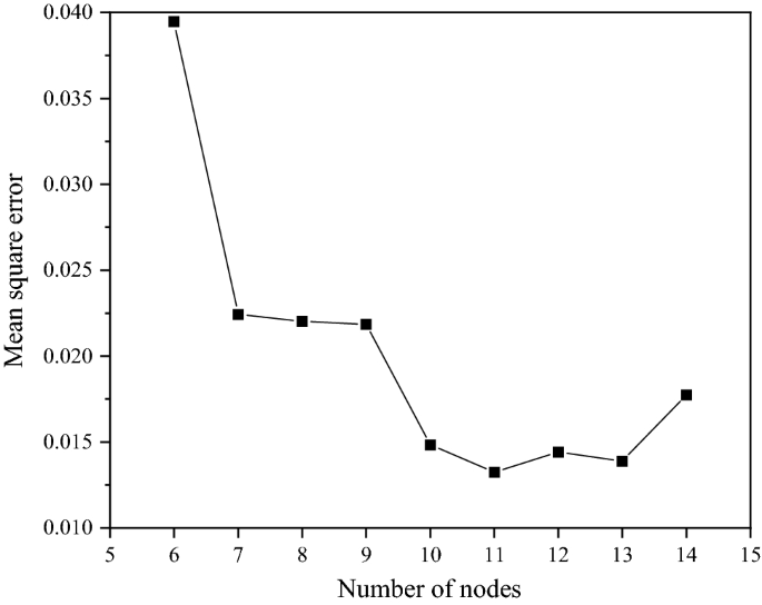
Relationship between mean square error and number of neuron nodes in hidden layer
-
(3)
The establishment, training and testing of BP neural networks. Based on the “newff” function in matlab, a three-layer neural network with the structure of "9–11-15" was established. The training function was Levenberg Marquardt algorithm. “Learngdm” and MSE were selected for the adaptive learning function and performance function. The transfer functions of the hidden and output layers were both “logsig”, and “trainParam.goal” was set to 0.001.

The training process of the BP neural network and the MSE are shown in Fig. 12. For the same dataset configuration, the recognition accuracy rate may change because the weight generated by each training was not a certain value, which was different from KNN and SVM. When shape and texture features were used as input, the average accuracy rate was 88.1% and 50.6%, respectively, and the highest accuracy rate was 89.9% and 55.7%, respectively. The highest recognition accuracy rate of BPNN was 94.9% when using fusion features as input.

Training process of BPNN (left) and mean square error of training (right)
The parameter selection of the BP-RBF network can be divided into two parts. The first is the parameter selection of the BP neural network. The parameters of BPNN are kept unchanged, and then the BPNN is connected with an RBF network. In the process of RBF network training, the most important parameter is “spread”. It is vital to select “spread” reasonably, and its value should be large enough to make the RBF neural network respond to the interval covered by the input vector, and make the prediction performance smoother. However, an overly large spread may cause numerical problems. The calculation of MSE and recognition accuracy rate with “spread” is shown in Fig. 13. When “spread” is in the range of 3.3–3.7, there is a small MSE and a large accuracy. Finally, 3.4 was selected as the ideal value of “spread”.When the 5, 4 and 9-dimensional features were imported into the BP-RBF neural network for training, the highest recognition accuracies of the test set were 88.6%, 49.4% and 96.2%, respectively. Compared with KNN, SVM and BPNN, the new BP-RBF hybrid neural network can improve the accuracy rate of leaf recognition.

Mean square error of recognition results and recognition accuracy of BP-RBF
Discussion
Table 4 shows the recognition accuracy rates of different classifiers, which provided the opportunity for performance comparisons. As can be seen, whether shape, texture or fusion features were used, BP-RBF had the highest recognition accuracy among all the methods. In contrast, SVM had the lowest. The BP-RBF network was used to optimize the previous methods, and the fusion feature recognition accuracy reached 96.2%, 1.3% higher than the BPNN. The contribution of various features to recognition rate can be compared by selecting shape and texture features as the input. When using texture features, the recognition rates of all methods were generally low (less than 50%). It's worth noting that the recognition rate was significantly improved after using texture features combined with shape features. This indicates that the contribution of shape features was obviously higher than that of texture features in this study. Therefore, it is necessary to fuse texture features with other types of features for plant identification.
According to Fig. 10, KNN and SVM were not able to recognize some specific types of leaves in the sample. The results of the above classifiers were unsatisfactory when identifying the tree species labeled 8, 11 and 12, while the other tree species were all recognized. The reason might be that the features of these plants are so similar to others that the current features are not enough to distinguish these leaves. The next task is to extract other suitable features to increase the differences between different kinds of plant leaves.
Up to now, researchers have proposed numerous effective methods for species recognition. Commonly used leaf recognition methods include PNN (Wu et al. 2007), LDC (Kalyoncu and Toygar 2015), GBDT-PNN (Tang 2020), and SVM (Salman et al. 2017; Ahmed and Hussein 2020). As seen in Table 5, the BP-RBF neural network achieved high performance in plant recognition systems using fewer samples and features.
Plant classification methods have great potential in forest studies and management. There were reports that plant identification error for professionals was 10–20% to the species level (Gray and Azuma 2005; Crall et al. 2011). Generally speaking, leaf structure allows closely related taxa to differentiate from each other (Merrill 1978; Sajo and Fls 2002; Espinosa et al. 2006). At the same time, leaf shape and texture are extracted from leaf structure. The system in this study can automatically preprocess leaf images, extract features, and realize the identification of the species. Its accuracy is comparable to the work of professionals, and can be used to develop a portable forest tree species recognition system helpful to non-professionals. The advantage is that the selected features are not affected by translation, rotation or scale of the leaf images. Although the recognition system proposed in this study has excellent performance, there is still room for improvement. Future work is to optimize the classification methods. On the one hand, the recognition performance of the system can be further improved by enriching the leaf features. On the other hand, more classification models and algorithms, such as convolutional neural network, require further exploration and experimentation. And the number of tree species in the dataset needs be increased.
Conclusion
This study used image processing technologies and machine learning algorithms to identify 15 kinds of plant leaves. A new BP-RBF hybrid neural network was proposed to further improve the recognition accuracy rate. The conclusions of this study are as follows.
In this study, a leaf database of common tree species in Northeast China was established. An image segmentation method, based on HSV color space and connected component labeling was presented, which can obtain the complete leaf image without veins and background. Leaf shape and texture were extracted using feature extraction algorithms. With all the leaf samples in our database, the recognition rates of KNN, SVM, BPNN and BP-RBF methods in the test set were 92.4%, 86.1%, 94.9% and 96.2%, respectively. Accordingly, the proposed BP-RBF hybrid algorithm had higher recognition accuracy than the other algorithms. For each method, the recognition contribution of shape features was greater than that of texture features. Compared with single-class features, the highest recognition rate can be obtained using fusion features. The BP-RBF neural network can achieve high recognition accuracy rates with fewer features and leaf samples compared with the other methods. In future studies, the performance of this proposed method will be improved by using other feature extraction techniques and classifiers.
References
Ahmed A, Hussein SE (2020) Leaf identification using radial basis function neural networks and SSA based support vector machine. PLoS ONE 15(8):e0237645
Backes AR, Casanova D, Bruno OM (2009) A complex network-based approach for boundary shape analysis. Pattern Recogn 42(1):54–67
Chang ZY, Cao J, Zhang YZ (2018) A novel image segmentation approach for wood plate surface defect classification through convex optimization. J for Res 29(6):1789–1795
Crall AW, Newman GJ, Stohlgren TJ, Holfelder KA, Graham J, Waller DM (2011) Assessing citizen science data quality: an invasive species case study. Conserv Lett 4(6):433–442
Espinosa D, Llorente J, Morrone JJ (2006) Historical biogeographical patterns of the species of Bursera (Burseraceae) and their taxonomic implications. J Biogeogr 33(11):1945–1958
Gong DX, Cao CR (2014) Classification of plant leaves based on convolutional neural network. Comput Mod 4:12–15
Gray AN, Azuma DL (2005) Repeatability and implementation of a forest vegetation indicator. Ecol Ind 5(1):57–71
Haralick RM, Shanmugam K, Dinstein IH (1973) Texture features for image classification. IEEE Trans Syst Man Cybern 3(6):610–621
Kalyoncu C, Toygar O (2015) Geometric leaf classification. Comput vis Image Underst 133:102–109
Kumar N, Belhumeur PN, Biswas A, Jacobs DW, Kress WJ, Lopez IC, Soares JVB (2012) Leafsnap: A computer vision system for automatic plant species identification. European Conference on Computer Vision, pp. 502–516
Larese MG, Namías R, Craviotto RM, Arango MR, Gallo C, Granitto PM (2014) Automatic classification of legumes using leaf vein image features. Pattern Recogn 47(1):158–168
Merrill E (1978) Comparison of mature leaf architecture of three types in Sorbus L. (Rosaceae). Bot Gaz 139(4):447–453
Muhammad AFA, Lee SC, Fakhrul RR, Farah IA, Sharifah RWA (2019) Review on techniques for plant leaf classification and recognition. Computers 8(4):77
Nelson JDB, Damper RI, Gunn SR, Guo B (2008) Signal theory for SVM kernel design with applications to parameter estimation and sequence kernels. Neurocomputing 72(1–3):15–22
Nevalainen O, Honkavaara E, Tuominen S, Viljanen N, Hakala T, Yu XW, Hyyppa J, Saari H, Polonen I, Imai NN, Tommaselli AMG (2017) Individual tree detection and classification with UAV-based photogrammetric point clouds and hyperspectral imaging. Remote Sensing 9(3):185
Otsu N (1979) A threshold selection method from gray-level histograms. IEEE Trans Syst Man Cybern 9(1):62–66
Perona P, Malik J (1990) Scale-space and edge detection using anisotropic diffusion. IEEE Trans Pattern Anal Mach Intell 12(7):629–639
Rahman MM, Islam MS, Sassi R, Aktaruzzaman M (2019) Convolutional neural networks performance comparison for handwritten Bengali numerals recognition. SN Appl Sci 1(12):1660
Roy K, Bhattacharya P (2010) Improvement of iris recognition performance using region-based active contours, genetic algorithms and SVMs. Int J Pattern Recognit Artif Intell 24(8):1209–1236
Rumelhart DE, Hinton GE, Williams RJ (1986) Learning representations by back-propagating errors. Nature 323(6088):533–536
Sajo MG, Rudall PJ (2002) Leaf and stem anatomy of Vochysiaceae in relation to subfamilial and suprafamilial systematics. Bot J Linn Soc 138(3):339–364
Salman A, Semwal A, Bhatt U, Thakkar VM (2017) Leaf classification and identification using Canny Edge Detector and SVM classifier. In: 2017 International Conference on Inventive Systems and Control (ICISC) pp. 1-4
Tang ZX (2020) Leaf image recognition and classification based on GBDT-probabilistic neural network. J Phys Conf Series 1592:012061
Tarjoman M, Fatemizadeh E, Badie K (2012) An implementation of a CBIR system based on SVM learning scheme. J Med Eng Technol 37(1):43–47
Turkoglu M, Hanbay D (2019) Recognition of plant leaves: an approach with hybrid features produced by dividing leaf images into two and four parts. Appl Math Comput 352:1–14
Wang XF, Huang DS, Du JX, Xu H, Heutte L (2008) Classification of plant leaf images with complicated background. Appl Math Comput 205(2):916–926
Wu SG, Bao FS, Xu EY, Wang YX, Xiang QL (2007) A leaf recognition algorithm for plant classification using probabilistic neural network. In: 2007 IEEE International Symposium on Signal Processing and Information Technology, pp. 11–16
Xu ZH, Huang XY, Lin L, Wang QF, Liu J, Yu KY, Chen CC (2018) BP neural networks and random forest models to detect damage by Dendrolimus punctatus Walker. J Forestry Res 31:107–121
Yang R, Kan J (2020) Classification of tree species at the leaf level based on hyperspectral imaging technology. J Appl Spectrosc 87(1):184–193
Yu HL, Liang YL, Liang H, Zhang YZ (2019) Recognition of wood surface defects with near infrared spectroscopy and machine vision. J Forestry Res 30:2379–2386
Zhang JW, Song WL, Jiang B, Li MB (2018) Measurement of lumber moisture content based on PCA and GS-SVM. J Forestry Res 29(2):1–8
Author information
Authors and Affiliations
Corresponding authors
Additional information
Publisher's Note
Springer Nature remains neutral with regard to jurisdictional claims in published maps and institutional affiliations.
Project funding
This work is supported by the Fundamental Research Funds for the Central Universities (No.2572020BC07) and the Project of National Science Foundation of China (No.31570712).
The online version is available at http://www.springerlink.com.
Corresponding editor: Yanbo Hu.
Rights and permissions
Open Access This article is licensed under a Creative Commons Attribution 4.0 International License, which permits use, sharing, adaptation, distribution and reproduction in any medium or format, as long as you give appropriate credit to the original author(s) and the source, provide a link to the Creative Commons licence, and indicate if changes were made. The images or other third party material in this article are included in the article's Creative Commons licence, unless indicated otherwise in a credit line to the material. If material is not included in the article's Creative Commons licence and your intended use is not permitted by statutory regulation or exceeds the permitted use, you will need to obtain permission directly from the copyright holder. To view a copy of this licence, visit http://creativecommons.org/licenses/by/4.0/.
About this article

Cite this article
Yang, X., Ni, H., Li, J. et al. Leaf recognition using BP-RBF hybrid neural network. J. For. Res. 33, 579–589 (2022). https://doi.org/10.1007/s11676-021-01362-4
Received:
Accepted:
Published:
Issue Date:
DOI: https://doi.org/10.1007/s11676-021-01362-4