


1 Introduction
Let X be a normed real vector space, and fix a correspondence
 $\Phi $
from X into itself and a functional
$\Phi $
from X into itself and a functional
 $u: X\to \mathbf {R}$
which may be interpreted as a utility function. Then, a sequence
$u: X\to \mathbf {R}$
which may be interpreted as a utility function. Then, a sequence
 $\boldsymbol {x}=(x_0,x_1,\ldots )$
with values in X is said to be feasible if
$\boldsymbol {x}=(x_0,x_1,\ldots )$
with values in X is said to be feasible if
 $x_{n+1}\in \Phi (x_n)$
, for all
$x_{n+1}\in \Phi (x_n)$
, for all
 $n\ge 0$
. Note that this sequence is simply the orbit of the starting point
$n\ge 0$
. Note that this sequence is simply the orbit of the starting point
 $x_0$
if
$x_0$
if
 $\Phi $
is singleton-valued. Fix also an ideal
$\Phi $
is singleton-valued. Fix also an ideal
 $\mathcal {I}$
on the nonnegative integers
$\mathcal {I}$
on the nonnegative integers
 $\mathbf {N}$
, which will represent the family of “small” sets (see Section 1.1 for definitions). Assuming that
$\mathbf {N}$
, which will represent the family of “small” sets (see Section 1.1 for definitions). Assuming that
 $\boldsymbol {x}$
belongs to a given constraint set
$\boldsymbol {x}$
belongs to a given constraint set
 $\mathscr {C}$
of feasible sequences, we say that
$\mathscr {C}$
of feasible sequences, we say that
 $\boldsymbol {x}$
is
$\boldsymbol {x}$
is
 $\mathcal {I}$
-optimal if it maximizes the smallest
$\mathcal {I}$
-optimal if it maximizes the smallest
 $\mathcal {I}$
-cluster point of the real sequence
$\mathcal {I}$
-cluster point of the real sequence
 $(u(x_0),u(x_1),\ldots )$
; here, an
$(u(x_0),u(x_1),\ldots )$
; here, an
 $\mathcal {I}$
-cluster point is, informally, an accumulation point which is not small with respect to
$\mathcal {I}$
-cluster point is, informally, an accumulation point which is not small with respect to
 $\mathcal {I}$
.
$\mathcal {I}$
.
Our aim is to study the asymptotic stability of
 $\mathcal {I}$
-optimal paths, which is often referred to as turnpike property (see, e.g., [Reference Zaslavski26, Reference Zaslavski27] for a textbook exposition). Roughly, this property states that an
$\mathcal {I}$
-optimal paths, which is often referred to as turnpike property (see, e.g., [Reference Zaslavski26, Reference Zaslavski27] for a textbook exposition). Roughly, this property states that an
 $\mathcal {I}$
-optimal path spends “most” of the time within a small neighborhood of some optimal stationary point, which is an identified fixed point of
$\mathcal {I}$
-optimal path spends “most” of the time within a small neighborhood of some optimal stationary point, which is an identified fixed point of
 $\Phi $
. Here, following the same lines of [Reference Das, Dutta, Mohiuddine and Alotaibi5, Reference Mamedov and Pehlivan20, Reference Pehlivan and Mamedov25], the adjective “most” is intended with respect to the ideal
$\Phi $
. Here, following the same lines of [Reference Das, Dutta, Mohiuddine and Alotaibi5, Reference Mamedov and Pehlivan20, Reference Pehlivan and Mamedov25], the adjective “most” is intended with respect to the ideal
 $\mathcal {I}$
. In particular,
$\mathcal {I}$
. In particular,
 $\mathcal {I}$
-optimal paths are potentially not convergent to the optimal stationary point. As remarked in [Reference Zaslavski26], the turnpike property has the following interpretation: if one is looking for an optimal way to reach A from B by car, then he should enter onto a turnpike, spend most of the time there, and finally leave the turnpike to reach the claimed point. There is an extensive literature which studies this phenomenon (see, e.g., [Reference Breiten and Pfeiffer3, Reference Damm, Grüne, Stieler and Worthmann4, Reference Gugat and Hante12, Reference Lewis and Paul18, Reference Mammadov and Evans21, Reference Marena and Montrucchio23]).
$\mathcal {I}$
-optimal paths are potentially not convergent to the optimal stationary point. As remarked in [Reference Zaslavski26], the turnpike property has the following interpretation: if one is looking for an optimal way to reach A from B by car, then he should enter onto a turnpike, spend most of the time there, and finally leave the turnpike to reach the claimed point. There is an extensive literature which studies this phenomenon (see, e.g., [Reference Breiten and Pfeiffer3, Reference Damm, Grüne, Stieler and Worthmann4, Reference Gugat and Hante12, Reference Lewis and Paul18, Reference Mammadov and Evans21, Reference Marena and Montrucchio23]).
Our main result (Theorem 2.1) generalizes the main ones obtained in [Reference Das, Dutta, Mohiuddine and Alotaibi5, Reference Mamedov and Pehlivan20]. We discuss later how our assumptions are related to the ones in these articles. In addition, we show with some novel examples that:
-
(i) The turnpike property provided in Theorem 2.1 does not hold without any restriction on the ideal
 $\mathcal {I}$
(see Example 2.3);
$\mathcal {I}$
(see Example 2.3); -
(ii) An
$\mathcal {I}$
-optimal path may not converge, in the classical sense, to the optimal stationary point (see Example 2.5); -
(iii) The turnpike property holds also in infinite dimension (see Example 5.1).


Our main result and its consequences follow in Section 2.
1.1 Preparation
An ideal
 $\mathcal {I}\subseteq \mathcal {P}(\mathbf {N})$
is a family closed under finite union and subsets. It is also assumed that
$\mathcal {I}\subseteq \mathcal {P}(\mathbf {N})$
is a family closed under finite union and subsets. It is also assumed that
 $\mathcal {I}$
contains the family of finite sets
$\mathcal {I}$
contains the family of finite sets
 $\mathrm {Fin}$
and it is different from
$\mathrm {Fin}$
and it is different from
 $\mathcal {P}(\mathbf {N})$
. Let also
$\mathcal {P}(\mathbf {N})$
. Let also
 $\mathcal {I}^\star :=\{S\subseteq \mathbf {N}: S^c\in \mathcal {I}\}$
be its dual filter and
$\mathcal {I}^\star :=\{S\subseteq \mathbf {N}: S^c\in \mathcal {I}\}$
be its dual filter and
 $\mathcal {I}^+:=\{S\subseteq \mathbf {N}: S\notin \mathcal {I}\}$
be the collection of
$\mathcal {I}^+:=\{S\subseteq \mathbf {N}: S\notin \mathcal {I}\}$
be the collection of
 $\mathcal {I}$
-positive sets. We denote by
$\mathcal {I}$
-positive sets. We denote by
 $\mathcal {Z}$
the ideal of asymptotic density zero sets, i.e.,
$\mathcal {Z}$
the ideal of asymptotic density zero sets, i.e.,
 $$ \begin{align*} \mathcal{Z}=\left\{A\subseteq \mathbf{N}: |\{a \in A: a\le n\}|=o(n) \text{ as }n\to \infty\right\}. \end{align*} $$
An ideal
 $\mathcal {I}$
on
$\mathcal {I}$
on
 $\mathbf {N}$
is said to be translation invariant if
$\mathbf {N}$
is said to be translation invariant if
 $(A+k) \cap \mathbf {N} \in \mathcal {I}$
for all
$(A+k) \cap \mathbf {N} \in \mathcal {I}$
for all
 $A \in \mathcal {I}$
and all (possibly negative) integers
$A \in \mathcal {I}$
and all (possibly negative) integers
 $k \in \mathbf {Z}$
. Note that the ideal
$k \in \mathbf {Z}$
. Note that the ideal
 $\mathcal {Z}$
is translation invariant. Classes of translation invariant ideals have been widely studied (see, e.g., [Reference Di Nasso and Jin6, Reference Filipów and Tryba9] and the ideals generated by the upper densities considered in [Reference Leonetti and Tringali17]). However, there exist ideals which are not translation invariant: for instance, all the maximal ideals (indeed, exactly one between the even and the odd integers belongs to a maximal ideal) and much simpler ones as the family of all sets
$\mathcal {Z}$
is translation invariant. Classes of translation invariant ideals have been widely studied (see, e.g., [Reference Di Nasso and Jin6, Reference Filipów and Tryba9] and the ideals generated by the upper densities considered in [Reference Leonetti and Tringali17]). However, there exist ideals which are not translation invariant: for instance, all the maximal ideals (indeed, exactly one between the even and the odd integers belongs to a maximal ideal) and much simpler ones as the family of all sets
 $A\subseteq \mathbf {N}$
containing finitely many even integers.
$A\subseteq \mathbf {N}$
containing finitely many even integers.
Let
 $\boldsymbol {x}=(x_n)$
be a sequence taking values in a topological vector space S. Then, we say that
$\boldsymbol {x}=(x_n)$
be a sequence taking values in a topological vector space S. Then, we say that
 $\boldsymbol {x}$
is
$\boldsymbol {x}$
is
 $\mathcal {I}$
-convergent to
$\mathcal {I}$
-convergent to
 $\eta \in S$
, shortened as
$\eta \in S$
, shortened as
 $\mathcal {I}\text {-}\lim \boldsymbol {x}=\eta $
, if
$\mathcal {I}\text {-}\lim \boldsymbol {x}=\eta $
, if
 $\{n \in \mathbf {N}: x_n \in U\} \in \mathcal {I}^\star $
for all open neighborhoods U of
$\{n \in \mathbf {N}: x_n \in U\} \in \mathcal {I}^\star $
for all open neighborhoods U of
 $\eta $
. Moreover, we say that
$\eta $
. Moreover, we say that
 $\eta \in S$
is an
$\eta \in S$
is an
 $\mathcal {I}$
-cluster point of
$\mathcal {I}$
-cluster point of
 $\boldsymbol {x}$
if
$\boldsymbol {x}$
if
 $\{n \in \mathbf {N}: x_n \in U\} \in \mathcal {I}^+$
for all open neighborhoods U of
$\{n \in \mathbf {N}: x_n \in U\} \in \mathcal {I}^+$
for all open neighborhoods U of
 $\eta $
. The set of
$\eta $
. The set of
 $\mathcal {I}$
-cluster points of
$\mathcal {I}$
-cluster points of
 $\boldsymbol {x}$
is denoted by
$\boldsymbol {x}$
is denoted by
 $\Gamma _{\boldsymbol {x}}(\mathcal {I})$
. Usually,
$\Gamma _{\boldsymbol {x}}(\mathcal {I})$
. Usually,
 $\mathcal {Z}$
-convergence and
$\mathcal {Z}$
-convergence and
 $\mathcal {Z}$
-cluster points are referred to as statistical convergence and statistical cluster points, respectively (see, e.g., [Reference Fridy10, Reference Miller24]). Note that
$\mathcal {Z}$
-cluster points are referred to as statistical convergence and statistical cluster points, respectively (see, e.g., [Reference Fridy10, Reference Miller24]). Note that
 $\mathrm {Fin}$
-convergence coincides with the ordinary convergence and that
$\mathrm {Fin}$
-convergence coincides with the ordinary convergence and that
 $\Gamma _{\boldsymbol {x}}(\mathrm {Fin})$
is the set of ordinary accumulation points of
$\Gamma _{\boldsymbol {x}}(\mathrm {Fin})$
is the set of ordinary accumulation points of
 $\boldsymbol {x}$
. It is worth noting that
$\boldsymbol {x}$
. It is worth noting that
 $\mathcal {I}$
-cluster points have been studied much before under a different name. Indeed, as it follows by [Reference Leonetti and Maccheroni16, Theorem 4.2] and [Reference Kadets and Seliutin14, Lemma 2.2], they correspond to classical “cluster points” of a filter (depending on
$\mathcal {I}$
-cluster points have been studied much before under a different name. Indeed, as it follows by [Reference Leonetti and Maccheroni16, Theorem 4.2] and [Reference Kadets and Seliutin14, Lemma 2.2], they correspond to classical “cluster points” of a filter (depending on
 $\boldsymbol {x}$
) on the underlying space (cf. [Reference Bourbaki2, Definition 2, p. 69]).
$\boldsymbol {x}$
) on the underlying space (cf. [Reference Bourbaki2, Definition 2, p. 69]).
Finally, following [Reference Fridy and Orhan11], for each real sequence
 $\boldsymbol {x}$
such that
$\boldsymbol {x}$
such that
 $\{n \in \mathbf {N}: |x_n|\ge M\}\in \mathcal {I}$
, for some
$\{n \in \mathbf {N}: |x_n|\ge M\}\in \mathcal {I}$
, for some
 $M \in \mathbf {R}$
, we define its
$M \in \mathbf {R}$
, we define its
 $\mathcal {I}$
-limit inferior as
$\mathcal {I}$
-limit inferior as
 $$ \begin{align*}\mathcal{I}\text{-}\liminf \boldsymbol{x}:=\inf\{r \in \mathbf{R}: \{n \in \mathbf{N}: x_n>r\}\in \mathcal{I}^+\}. \end{align*} $$
Simmetrically, we let
 $\mathcal {I}\text {-}\limsup \boldsymbol {x}:=-\mathcal {I}\text {-}\liminf (-\boldsymbol {x})$
be the
$\mathcal {I}\text {-}\limsup \boldsymbol {x}:=-\mathcal {I}\text {-}\liminf (-\boldsymbol {x})$
be the
 $\mathcal {I}$
-limit superior. Again, it is easy to see that if
$\mathcal {I}$
-limit superior. Again, it is easy to see that if
 $\mathcal {I}=\mathrm {Fin}$
, then they coincide with the ordinary limit inferior and limit superior of
$\mathcal {I}=\mathrm {Fin}$
, then they coincide with the ordinary limit inferior and limit superior of
 $\boldsymbol {x}$
, respectively. It is remarkable that they can be rewritten also as the smallest and the biggest
$\boldsymbol {x}$
, respectively. It is remarkable that they can be rewritten also as the smallest and the biggest
 $\mathcal {I}$
-cluster points of
$\mathcal {I}$
-cluster points of
 $\boldsymbol {x}$
, respectively (cf. Corollary 3.3 below).
$\boldsymbol {x}$
, respectively (cf. Corollary 3.3 below).
Given sets
 $A,B$
, we say that
$A,B$
, we say that
 $\alpha : A\rightrightarrows B$
is a correspondence if
$\alpha : A\rightrightarrows B$
is a correspondence if
 $\alpha (x)$
is a (possibly empty) subset of B for each
$\alpha (x)$
is a (possibly empty) subset of B for each
 $x \in A$
. Moreover, we denote the set of its fixed points by
$x \in A$
. Moreover, we denote the set of its fixed points by
 $$ \begin{align*}\mathrm{Fix}(\alpha):=\{x \in A: x \in \alpha(x)\}. \end{align*} $$
We recall that, if A and B are endowed with some topologies, then the correspondence
 $\alpha $
is upper hemicontinuous at
$\alpha $
is upper hemicontinuous at
 $x \in A$
if for each open
$x \in A$
if for each open
 $U\supseteq \alpha (x)$
, there exists an open neighborhood V of x such that
$U\supseteq \alpha (x)$
, there exists an open neighborhood V of x such that
 $z \in V$
implies
$z \in V$
implies
 $\varphi (z)\subseteq U$
. Moreover,
$\varphi (z)\subseteq U$
. Moreover,
 $\alpha $
is lower hemicontinuous at
$\alpha $
is lower hemicontinuous at
 $x \in A$
if for every open
$x \in A$
if for every open
 $U\subseteq B$
with
$U\subseteq B$
with
 $\varphi (x)\cap U\neq \emptyset $
, there exists an open neighborhood V of x such that
$\varphi (x)\cap U\neq \emptyset $
, there exists an open neighborhood V of x such that
 $z \in V$
implies
$z \in V$
implies
 $\varphi (z)\cap U\neq \emptyset $
. Finally, the correspondence
$\varphi (z)\cap U\neq \emptyset $
. Finally, the correspondence
 $\alpha $
is said to be continuous if it is both upper and lower hemicontinuous at each point
$\alpha $
is said to be continuous if it is both upper and lower hemicontinuous at each point
 $x \in A$
(see [Reference Aliprantis and Border1, Definition 17.2]).
$x \in A$
(see [Reference Aliprantis and Border1, Definition 17.2]).
Given a function
 $h: A\to B$
and a sequence
$h: A\to B$
and a sequence
 $\boldsymbol {x}=(x_0,x_1,\ldots )$
with values in A, we write
$\boldsymbol {x}=(x_0,x_1,\ldots )$
with values in A, we write
 $h(\boldsymbol {x})$
for the sequence
$h(\boldsymbol {x})$
for the sequence
 $(h(x_0), h(x_1), \ldots )$
. Finally, if
$(h(x_0), h(x_1), \ldots )$
. Finally, if
 $B=\mathbf {R}$
, we say that
$B=\mathbf {R}$
, we say that
 $x_0 \in A$
is a maximizer of h if
$x_0 \in A$
is a maximizer of h if
 $h(x) \le h(x_0)$
, for all
$h(x) \le h(x_0)$
, for all
 $x \in A$
(and similarly for minimizers).
$x \in A$
(and similarly for minimizers).
2 Main result
Let X be a real normed vector space and denote by
 $\mathcal {K}$
the collection of its nonempty compact subsets. In addition, let
$\mathcal {K}$
the collection of its nonempty compact subsets. In addition, let
 $\mathcal {I}$
be an ideal on the nonnegative integers
$\mathcal {I}$
be an ideal on the nonnegative integers
 $\mathbf {N}$
, and fix a correspondence
$\mathbf {N}$
, and fix a correspondence
 $ \Phi : X\rightrightarrows X $
and a function
$ \Phi : X\rightrightarrows X $
and a function
 $ u: X\to \mathbf {R}. $
In this setting, the function u will take the role of a utility function which induces a total preorder on X.
$ u: X\to \mathbf {R}. $
In this setting, the function u will take the role of a utility function which induces a total preorder on X.
Let
 $\mathscr {K}$
be the family of sequences
$\mathscr {K}$
be the family of sequences
 $\boldsymbol {x}=(x_0,x_1,\ldots )$
taking values in X which are
$\boldsymbol {x}=(x_0,x_1,\ldots )$
taking values in X which are
 $\mathcal {I}$
-contained in a compact, that is, such that
$\mathcal {I}$
-contained in a compact, that is, such that
 $\{n \in \mathbf {N}: x_n \notin K\}\in \mathcal {I}$
, for some
$\{n \in \mathbf {N}: x_n \notin K\}\in \mathcal {I}$
, for some
 $K\in \mathcal {K}$
. Moreover, we let
$K\in \mathcal {K}$
. Moreover, we let
 $\mathscr {F}$
be the collection of feasible paths
$\mathscr {F}$
be the collection of feasible paths
 $\boldsymbol {x}$
which satisfy
$\boldsymbol {x}$
which satisfy
 $x_{n+1} \in \Phi (x_n)$
, for all n, that is,
$x_{n+1} \in \Phi (x_n)$
, for all n, that is,
 $$ \begin{align*}\mathscr{F}=\{\boldsymbol{x} \in X^{\mathbf{N}}: \forall n \in \mathbf{N}, x_{n+1} \in \Phi(x_n) \}. \end{align*} $$
It is easy to see that, if u is continuous, then
 $\mathcal {I}\text {-}\liminf u(\boldsymbol {x})$
and
$\mathcal {I}\text {-}\liminf u(\boldsymbol {x})$
and
 $\mathcal {I}\text {-}\limsup u(\boldsymbol {x})$
are well defined for each sequence
$\mathcal {I}\text {-}\limsup u(\boldsymbol {x})$
are well defined for each sequence
 $\boldsymbol {x} \in \mathscr {F}_{\mathrm {K}}$
, where
$\boldsymbol {x} \in \mathscr {F}_{\mathrm {K}}$
, where
 $$ \begin{align*}\mathscr{F}_{\mathrm{K}}:=\mathscr{F} \cap \mathscr{K} \end{align*} $$
(cf. Section 3). Fix also a nonempty subset
 $\mathscr {C}\subseteq \mathscr {F}_{\mathrm {K}}$
, which will take the role of the collection of constraints. Note that the primitive elements of this system are represented by the tuple
$\mathscr {C}\subseteq \mathscr {F}_{\mathrm {K}}$
, which will take the role of the collection of constraints. Note that the primitive elements of this system are represented by the tuple
 $ \langle X, \Phi , u, \mathcal {I}, \mathscr {C}\rangle . $
Finally, we say that a sequence
$ \langle X, \Phi , u, \mathcal {I}, \mathscr {C}\rangle . $
Finally, we say that a sequence
 $\boldsymbol {x} \in \mathscr {C}$
is
$\boldsymbol {x} \in \mathscr {C}$
is
 $\boldsymbol {\mathcal {I}}$
-optimal if
$\boldsymbol {\mathcal {I}}$
-optimal if
 $$ \begin{align} \textstyle \forall \boldsymbol{y} \in \mathscr{C}, \quad \mathcal{I}\text{-}\liminf u(\boldsymbol{x}) \ge \mathcal{I}\text{-}\liminf u(\boldsymbol{y}). \end{align} $$
In other words, an
 $\mathcal {I}$
-optimal path
$\mathcal {I}$
-optimal path
 $\boldsymbol {x}$
is a maxmin solution in a precise sense: it maximizes the minimal
$\boldsymbol {x}$
is a maxmin solution in a precise sense: it maximizes the minimal
 $\mathcal {I}$
-cluster point of the sequence
$\mathcal {I}$
-cluster point of the sequence
 $(u(y_0), u(y_1),\ldots )$
among all feasible paths
$(u(y_0), u(y_1),\ldots )$
among all feasible paths
 $\boldsymbol {y}$
in the constraint set
$\boldsymbol {y}$
in the constraint set
 $\mathscr {C}$
(cf. Corollary 3.3 below).
$\mathscr {C}$
(cf. Corollary 3.3 below).
The aim of this work, in the same spirit of [Reference Das, Dutta, Mohiuddine and Alotaibi5, Reference Mamedov and Pehlivan20, Reference Mammadov and Evans21, Reference Pehlivan and Mamedov25], is to find sufficient conditions on the system
 $\langle X, \Phi , u, \mathcal {I}, \mathscr {C}\rangle $
such that every
$\langle X, \Phi , u, \mathcal {I}, \mathscr {C}\rangle $
such that every
 $\mathcal {I}$
-optimal path is necessarily
$\mathcal {I}$
-optimal path is necessarily
 $\mathcal {I}$
-convergent to some identified fixed point of
$\mathcal {I}$
-convergent to some identified fixed point of
 $\Phi $
(in this setting, a fixed point of
$\Phi $
(in this setting, a fixed point of
 $\Phi $
is usually called stationary point). We are going to show that certain feasible paths satisfy this property whenever the following conditions on
$\Phi $
is usually called stationary point). We are going to show that certain feasible paths satisfy this property whenever the following conditions on
 $\langle X, \Phi , u, \mathcal {I}, \mathscr {C}\rangle $
hold:
$\langle X, \Phi , u, \mathcal {I}, \mathscr {C}\rangle $
hold:
-
(A1)
$\Phi $
is continuous and takes values in
$\mathcal {K}$
; -
(A2) u is continuous;
-
(A3)
$\mathcal {I}$
is translation invariant; -
(A4) There exists a unique
$\eta ^\star \in \mathrm {Fix}(\Phi )$
which maximizes the restriction of u on
$\mathrm {Fix}(\Phi )$
; -
(A5) There exists a continuous linear functional
$T: X\to \mathbf {R}$
such that (2.2)where
$$ \begin{align} \forall x \in F, \forall y \in \Phi(x), \quad Tx \le Ty \implies x=y=\eta^\star\textrm{,} \end{align} $$
$F:=\{x \in X: u(x) \ge u(\eta ^\star )\}$
;
-
(A6)
$\sup _{\boldsymbol {y} \in \mathscr {C}} \mathcal {I}\text {-}\liminf u(\boldsymbol {y}) \ge u(\eta ^\star )$
.


We remark that condition (A1) is equivalent to the fact that the function
 $X\to \mathcal {K}$
defined by
$X\to \mathcal {K}$
defined by
 $x\mapsto \Phi (x)$
is continuous with respect to the Hausdorff metric (see [Reference Aliprantis and Border1, Theorem 17.15]).
$x\mapsto \Phi (x)$
is continuous with respect to the Hausdorff metric (see [Reference Aliprantis and Border1, Theorem 17.15]).
Note that the separation property given in condition (A5) has been already used in [Reference Das, Dutta, Mohiuddine and Alotaibi5, Reference Mamedov and Pehlivan20] for the case
 $X=\mathbf {R}^n$
, replacing (2.2) with the weaker variant
$X=\mathbf {R}^n$
, replacing (2.2) with the weaker variant
 $$ \begin{align} \forall x \in F, \forall y \in \Phi(x), \quad Tx \le Ty \implies x=\eta^\star\textrm{.} \end{align} $$
However, a careful analysis of their proofs reveals that, in fact, they were both implicitly using (2.2). Indeed, as pointed out by Piotr Szuca in a private communication [Reference Mammadov and Szuca22], condition (2.3) is, in fact, not sufficient for their purposes. On this direction, see also Remark 4.1 below. Condition (2.3) appeared also in [Reference Mamedov19] in the study of turnpike theorems for integral functionals in a continuous time setting. A somehow related condition can be found in [Reference Mammadov and Evans21, Lemma 4.3].
Our main result follows.
Theorem 2.1 Let
 $\langle X, \Phi , u, \mathcal {I}, \mathscr {C}\rangle $
be a system which satisfies conditions (A1)–(A6). Let also
$\langle X, \Phi , u, \mathcal {I}, \mathscr {C}\rangle $
be a system which satisfies conditions (A1)–(A6). Let also
 $\boldsymbol {x}\in \mathscr {C}$
be an
$\boldsymbol {x}\in \mathscr {C}$
be an
 $\mathcal {I}$
-optimal path. Then,
$\mathcal {I}$
-optimal path. Then,
 $\mathcal {I}\text {-}\lim \boldsymbol {x}=\eta ^\star $
.
$\mathcal {I}\text {-}\lim \boldsymbol {x}=\eta ^\star $
.
It is worth to remark that, differently from most of the literature on turnpike theorems, we do not assume neither the concavity of the utility function u nor the convexity of the images
 $\Phi (x)$
, for each
$\Phi (x)$
, for each
 $x \in X$
. Moreover, a sufficient condition to imply condition (A6) is the existence of a sequence
$x \in X$
. Moreover, a sufficient condition to imply condition (A6) is the existence of a sequence
 $\boldsymbol {y} \in \mathscr {C}$
which is
$\boldsymbol {y} \in \mathscr {C}$
which is
 $\mathcal {I}$
-convergent to
$\mathcal {I}$
-convergent to
 $\eta ^\star $
, which gives us the following corollary.
$\eta ^\star $
, which gives us the following corollary.
Corollary 2.2 Let
 $\langle X, \Phi , u, \mathcal {I}, \mathscr {C}\rangle $
be a system which satisfies conditions (A1)–(A5) and suppose that there exists
$\langle X, \Phi , u, \mathcal {I}, \mathscr {C}\rangle $
be a system which satisfies conditions (A1)–(A5) and suppose that there exists
 $\boldsymbol {y} \in \mathscr {C}$
such that
$\boldsymbol {y} \in \mathscr {C}$
such that
 $\mathcal {I}\text {-}\lim \boldsymbol {y}=\eta ^\star $
. Let also
$\mathcal {I}\text {-}\lim \boldsymbol {y}=\eta ^\star $
. Let also
 $\boldsymbol {x} \in \mathscr {C}$
be an
$\boldsymbol {x} \in \mathscr {C}$
be an
 $\mathcal {I}$
-optimal path. Then,
$\mathcal {I}$
-optimal path. Then,
 $\mathcal {I}\text {-}\lim \boldsymbol {x}=\eta ^\star $
.
$\mathcal {I}\text {-}\lim \boldsymbol {x}=\eta ^\star $
.
Corollary 2.2 generalizes the main results obtained in [Reference Das, Dutta, Mohiuddine and Alotaibi5, Reference Mamedov and Pehlivan20]. Indeed, in [Reference Mamedov and Pehlivan20], Mamedov and Pehlivan assumed, in addition, that: X is the finite dimensional vector space
 $\mathbf {R}^k$
, F is compact, there exists a compact set containing (the image of) each feasible sequence in
$\mathbf {R}^k$
, F is compact, there exists a compact set containing (the image of) each feasible sequence in
 $\mathscr {F}_{\mathrm {K}}$
, the set of contraints
$\mathscr {F}_{\mathrm {K}}$
, the set of contraints
 $\mathscr {C}$
depends on the sequence
$\mathscr {C}$
depends on the sequence
 $\boldsymbol {x}$
, so that
$\boldsymbol {x}$
, so that
 $\mathscr {C}$
is of the type
$\mathscr {C}$
is of the type
 $\{\boldsymbol {z} \in \mathscr {F}_{\mathrm {K}}: x_0=z_0\}$
, and there exists
$\{\boldsymbol {z} \in \mathscr {F}_{\mathrm {K}}: x_0=z_0\}$
, and there exists
 $\boldsymbol {y}\in \mathscr {C}$
which is convergent to
$\boldsymbol {y}\in \mathscr {C}$
which is convergent to
 $\eta ^\star $
(in the place of the weaker assumption of
$\eta ^\star $
(in the place of the weaker assumption of
 $\mathcal {I}$
-convergence). The same hypotheses have been also used by Das et al. in [Reference Das, Dutta, Mohiuddine and Alotaibi5], where the authors considered certain correspondences
$\mathcal {I}$
-convergence). The same hypotheses have been also used by Das et al. in [Reference Das, Dutta, Mohiuddine and Alotaibi5], where the authors considered certain correspondences
 $\Phi : \mathbf {R}^k \rightrightarrows \mathbf {R}^k$
such that
$\Phi : \mathbf {R}^k \rightrightarrows \mathbf {R}^k$
such that
 $\Phi (x)=\{h(x,y): y \in U\}$
, for all
$\Phi (x)=\{h(x,y): y \in U\}$
, for all
 $x \in \mathbf {R}^k$
, where
$x \in \mathbf {R}^k$
, where
 $h: \mathbf {R}^k \to \mathbf {R}^m$
is a continuous function and
$h: \mathbf {R}^k \to \mathbf {R}^m$
is a continuous function and
 $U\subseteq \mathbf {R}^m$
is a fixed nonempty compact set (it is routine to show that all correspondences
$U\subseteq \mathbf {R}^m$
is a fixed nonempty compact set (it is routine to show that all correspondences
 $\Phi $
of this type are continuous). Finally, Mamedov and Pehlivan [Reference Mamedov and Pehlivan20] focused on the case
$\Phi $
of this type are continuous). Finally, Mamedov and Pehlivan [Reference Mamedov and Pehlivan20] focused on the case
 $\mathcal {I}=\mathcal {Z}$
. Hence, Corollary 2.2 proves that all these assumptions are not really needed.
$\mathcal {I}=\mathcal {Z}$
. Hence, Corollary 2.2 proves that all these assumptions are not really needed.
In the next example, we show that Corollary 2.2 (and, hence, also Theorem 2.1) cannot be extended to all the ideals
 $\mathcal {I}$
.
$\mathcal {I}$
.
Example 2.3 Let
 $\mathcal {I}$
be an ideal on
$\mathcal {I}$
be an ideal on
 $\mathbf {N}$
such that
$\mathbf {N}$
such that
 $2\mathbf {N}\subseteq \mathcal {I}$
. Note that such ideals exist, e.g., the family of subsets of
$2\mathbf {N}\subseteq \mathcal {I}$
. Note that such ideals exist, e.g., the family of subsets of
 $\mathbf {N}$
containing finitely many odd integers, or the maximal ideals extending
$\mathbf {N}$
containing finitely many odd integers, or the maximal ideals extending
 $2\mathbf {N}$
. Now, let
$2\mathbf {N}$
. Now, let
 $X=\mathbf {R}$
, and define
$X=\mathbf {R}$
, and define
![]() and
and
 $u(x)=x^3$
, for each
$u(x)=x^3$
, for each
 $x \in \mathbf {R}$
. Moreover, set
$x \in \mathbf {R}$
. Moreover, set
 $\mathscr {C}:=\{\boldsymbol {y} \in \mathscr {F}_{\mathrm {K}}: y_0=1\}$
. Then, the continuous correspondence
$\mathscr {C}:=\{\boldsymbol {y} \in \mathscr {F}_{\mathrm {K}}: y_0=1\}$
. Then, the continuous correspondence
 $\Phi $
has a unique fixed point, i.e.,
$\Phi $
has a unique fixed point, i.e.,
 $\mathrm {Fix}(\Phi )=\{0\}$
. It is easily seen that the system
$\mathrm {Fix}(\Phi )=\{0\}$
. It is easily seen that the system
 $\langle X, \Phi , u, \mathcal {I}, \mathscr {C}\rangle $
satisfies conditions (A1)–(A4). Moreover, also condition (A5) holds: indeed, notice that
$\langle X, \Phi , u, \mathcal {I}, \mathscr {C}\rangle $
satisfies conditions (A1)–(A4). Moreover, also condition (A5) holds: indeed, notice that
 $F=\{x \in \mathbf {R}: u(x) \ge u(0)\}=[0,\infty )$
. Then, setting
$F=\{x \in \mathbf {R}: u(x) \ge u(0)\}=[0,\infty )$
. Then, setting
 $T(r)=r$
, for all
$T(r)=r$
, for all
 $r \in \mathbf {R}$
, we obtain that
$r \in \mathbf {R}$
, we obtain that
 $Ty<Tx$
for all
$Ty<Tx$
for all
 $(x,y) \neq (0,0)$
with
$(x,y) \neq (0,0)$
with
 $x \in F$
and
$x \in F$
and
 $y \in \Phi (x)$
, i.e., for all
$y \in \Phi (x)$
, i.e., for all
 $x>0$
and
$x>0$
and
![]() .
.
At this point, let
 $\boldsymbol {x}=(x_0,x_1,\ldots )\in \mathscr {C}$
be the sequence defined by
$\boldsymbol {x}=(x_0,x_1,\ldots )\in \mathscr {C}$
be the sequence defined by
 $x_n=(-1)^{n}$
, for all
$x_n=(-1)^{n}$
, for all
 $n \in \mathbf {N}$
. Then,
$n \in \mathbf {N}$
. Then,
 $\boldsymbol {x} \in \mathscr {C}$
and
$\boldsymbol {x} \in \mathscr {C}$
and
 $u(\boldsymbol {x})=\boldsymbol {x}$
, so that
$u(\boldsymbol {x})=\boldsymbol {x}$
, so that
 $\mathcal {I}\text {-}\lim u(\boldsymbol {x})=1$
. Because
$\mathcal {I}\text {-}\lim u(\boldsymbol {x})=1$
. Because
 $|u(y_n)|\le 1$
, for all
$|u(y_n)|\le 1$
, for all
 $\boldsymbol {y} \in \mathscr {C}$
and
$\boldsymbol {y} \in \mathscr {C}$
and
 $n \in \mathbf {N}$
, it follows that
$n \in \mathbf {N}$
, it follows that
 $\boldsymbol {x}$
is
$\boldsymbol {x}$
is
 $\mathcal {I}$
-optimal. In addition, the sequence
$\mathcal {I}$
-optimal. In addition, the sequence
 $\boldsymbol {y}$
defined by
$\boldsymbol {y}$
defined by
 $y_n=2^{-n}$
, for all
$y_n=2^{-n}$
, for all
 $n \in \mathbf {N}$
, belongs to
$n \in \mathbf {N}$
, belongs to
 $\mathscr {C}$
, and it is convergent (in the classical sense) to
$\mathscr {C}$
, and it is convergent (in the classical sense) to
 $0$
. Hence, all hypotheses of Corollary 2.2 hold. However, the sequence
$0$
. Hence, all hypotheses of Corollary 2.2 hold. However, the sequence
 $\boldsymbol {x}$
is clearly not
$\boldsymbol {x}$
is clearly not
 $\mathcal {I}$
-convergent to
$\mathcal {I}$
-convergent to
 $0$
.
$0$
.
Note that the same construction given in Example 2.3 does not contradict Corollary 2.2 in the case that
 $\mathcal {I}$
is a translation invariant ideal. Indeed, in such case,
$\mathcal {I}$
is a translation invariant ideal. Indeed, in such case,
 $2\mathbf {N} \in \mathcal {I}$
if and only if
$2\mathbf {N} \in \mathcal {I}$
if and only if
 $2\mathbf {N}+1\in \mathcal {I}$
. However, because their union is
$2\mathbf {N}+1\in \mathcal {I}$
. However, because their union is
 $\mathbf {N}$
, then they are both
$\mathbf {N}$
, then they are both
 $\mathcal {I}$
-positive sets, so that
$\mathcal {I}$
-positive sets, so that
 $\Gamma _{u(\boldsymbol {x})}(\mathcal {I})=\{1,-1\}$
and
$\Gamma _{u(\boldsymbol {x})}(\mathcal {I})=\{1,-1\}$
and
 $\mathcal {I}\text {-}\liminf u(\boldsymbol {x})=-1$
. Therefore,
$\mathcal {I}\text {-}\liminf u(\boldsymbol {x})=-1$
. Therefore,
 $\boldsymbol {x}$
would be not
$\boldsymbol {x}$
would be not
 $\mathcal {I}$
-optimal. Moreover, this provides an example of a system
$\mathcal {I}$
-optimal. Moreover, this provides an example of a system
 $\langle X, \Phi , u, \mathcal {I}, \mathscr {C}\rangle $
such that u is neither concave nor convex,
$\langle X, \Phi , u, \mathcal {I}, \mathscr {C}\rangle $
such that u is neither concave nor convex,
 $\Phi $
is not convex-valued, and F is not compact.
$\Phi $
is not convex-valued, and F is not compact.
Suppose now that
 $\Phi $
is singleton-valued, that is, there exists a function
$\Phi $
is singleton-valued, that is, there exists a function
 $\phi : X\to X$
such that
$\phi : X\to X$
such that
 $\Phi (x)=\{\phi (x)\}$
, for all
$\Phi (x)=\{\phi (x)\}$
, for all
 $x \in X$
. Note that the continuity of
$x \in X$
. Note that the continuity of
 $\Phi $
in condition (A1) is equivalent to the continuity of
$\Phi $
in condition (A1) is equivalent to the continuity of
 $\phi $
(see [Reference Aliprantis and Border1, Lemma 17.6]). Here, let us identify
$\phi $
(see [Reference Aliprantis and Border1, Lemma 17.6]). Here, let us identify
 $\Phi $
with
$\Phi $
with
 $\phi $
. Notice also that a feasible sequence
$\phi $
. Notice also that a feasible sequence
 $\boldsymbol {x} \in \mathscr {F}$
is simply an orbit
$\boldsymbol {x} \in \mathscr {F}$
is simply an orbit
 $(x_0, \phi (x_0), \phi ^2(x_0), \ldots )$
. Hence, the constraint set
$(x_0, \phi (x_0), \phi ^2(x_0), \ldots )$
. Hence, the constraint set
 $\mathscr {C}$
can be identified with the set of starting values
$\mathscr {C}$
can be identified with the set of starting values
 $C:=\{x \in X: \exists \boldsymbol {x} \in \mathscr {C}, x_0=x\}$
. To sum up, the system can be identified with the tuple
$C:=\{x \in X: \exists \boldsymbol {x} \in \mathscr {C}, x_0=x\}$
. To sum up, the system can be identified with the tuple
 $\langle X, \phi , u, \mathcal {I}, C\rangle $
, and a sequence
$\langle X, \phi , u, \mathcal {I}, C\rangle $
, and a sequence
 $\boldsymbol {x}$
with
$\boldsymbol {x}$
with
 $x_0 \in C$
is
$x_0 \in C$
is
 $\mathcal {I}$
-optimal provided that
$\mathcal {I}$
-optimal provided that
 $$ \begin{align*} \textstyle \forall y \in C, \quad \mathcal{I}\text{-}\liminf_{n} u(\phi^n(x_0)) \ge \mathcal{I}\text{-}\liminf_{n} u(\phi^n(y)), \end{align*} $$
where
 $\phi ^0(x):=x$
, for all
$\phi ^0(x):=x$
, for all
 $x \in X$
. With these premises, we have the following corollary.
$x \in X$
. With these premises, we have the following corollary.
Corollary 2.4 Let
 $\langle X, \phi , u, \mathcal {I}, C\rangle $
be a system which satisfies conditions (A1)–(A5), and suppose that there exists
$\langle X, \phi , u, \mathcal {I}, C\rangle $
be a system which satisfies conditions (A1)–(A5), and suppose that there exists
 $y_0 \in C$
such that
$y_0 \in C$
such that
 $\liminf _n u(\phi ^n(y_0))\ge u(\eta ^\star )$
. Fix also
$\liminf _n u(\phi ^n(y_0))\ge u(\eta ^\star )$
. Fix also
 $x_0 \in X$
such that the orbit
$x_0 \in X$
such that the orbit
 $(\phi ^n(x_0))$
is
$(\phi ^n(x_0))$
is
 $\mathcal {I}$
-optimal. Then,
$\mathcal {I}$
-optimal. Then,
 $\mathcal {I}\text {-}\lim _n \phi ^n(x_0)=\eta ^\star $
.
$\mathcal {I}\text {-}\lim _n \phi ^n(x_0)=\eta ^\star $
.
At this point, one may wonder if the standing assumptions of Theorem 2.1 together with the
 $\mathcal {I}$
-optimality of the sequence
$\mathcal {I}$
-optimality of the sequence
 $\boldsymbol {x}$
imply the stronger conclusion that
$\boldsymbol {x}$
imply the stronger conclusion that
 $\lim \boldsymbol {x}=\eta ^\star $
, so that, in a sense, it would be not necessary to speak about ideals. In the next example, we show that this is not the case. Indeed, there exists a system
$\lim \boldsymbol {x}=\eta ^\star $
, so that, in a sense, it would be not necessary to speak about ideals. In the next example, we show that this is not the case. Indeed, there exists a system
 $\langle X, \Phi , u, \mathcal {I}, \mathscr {C}\rangle $
which satisfies conditions (A1)–(A6) and an
$\langle X, \Phi , u, \mathcal {I}, \mathscr {C}\rangle $
which satisfies conditions (A1)–(A6) and an
 $\mathcal {I}$
-optimal sequence
$\mathcal {I}$
-optimal sequence
 $\boldsymbol {x} \in \mathscr {C}$
which is not convergent in the ordinary sense (however, thanks to Theorem 2.1, it is
$\boldsymbol {x} \in \mathscr {C}$
which is not convergent in the ordinary sense (however, thanks to Theorem 2.1, it is
 $\mathcal {I}$
-convergent to
$\mathcal {I}$
-convergent to
 $\eta ^\star $
).
$\eta ^\star $
).
Example 2.5 Set
 $X=\mathbf {R}$
,
$X=\mathbf {R}$
,
 $\mathcal {I}=\mathcal {Z}$
,
$\mathcal {I}=\mathcal {Z}$
,
 $\mathscr {C}=\mathscr {F}_{\mathrm {K}}$
,
$\mathscr {C}=\mathscr {F}_{\mathrm {K}}$
,
 $\Phi (x):=[-2x,-\frac {x}{2}]$
, and
$\Phi (x):=[-2x,-\frac {x}{2}]$
, and
 $u(x)=x$
, for all
$u(x)=x$
, for all
 $x \in \mathbf {R}$
. It is not difficult to see that conditions (A1)–(A6) hold, and
$x \in \mathbf {R}$
. It is not difficult to see that conditions (A1)–(A6) hold, and
 $\mathrm {Fix}(\Phi )=\{0\}$
(cf. Example 2.3).
$\mathrm {Fix}(\Phi )=\{0\}$
(cf. Example 2.3).
At this point, let
 $\boldsymbol {x}=(x_0,x_1,\ldots )$
be the sequence for which
$\boldsymbol {x}=(x_0,x_1,\ldots )$
be the sequence for which
 $\text{for all }n x_n=(-1)^nz_n$
, where
$\text{for all }n x_n=(-1)^nz_n$
, where
 $\boldsymbol {z}=(z_0,z_1,\ldots )$
is defined as it follows:
$\boldsymbol {z}=(z_0,z_1,\ldots )$
is defined as it follows:
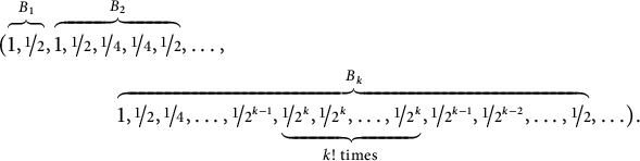
Here, for each
 $k\ge 1$
, the block
$k\ge 1$
, the block
 $B_k$
has
$B_k$
has
 $2k-1+k!$
terms and its middle part is made by
$2k-1+k!$
terms and its middle part is made by
 $k!$
consecutive terms equal to
$k!$
consecutive terms equal to
.
Let us show that
 $\boldsymbol {x}$
is
$\boldsymbol {x}$
is
 $\mathcal {Z}$
-optimal: first of all, using the fact that
$\mathcal {Z}$
-optimal: first of all, using the fact that
 $$ \begin{align*}\textstyle \sum_{k\le n-1}|B_k| \le \sum_{k\le n-1}3\cdot (k-1)!=o(n!) \text{ as }n\to \infty, \end{align*} $$
thus
 $\mathcal {Z}\text {-}\lim \boldsymbol {x}=0$
(cf. also [Reference Leonetti and Tringali17, Lemma 1]). In particular,
$\mathcal {Z}\text {-}\lim \boldsymbol {x}=0$
(cf. also [Reference Leonetti and Tringali17, Lemma 1]). In particular,
 $\mathcal {Z}\text {-}\liminf \boldsymbol {x}=\mathcal {Z}\text {-}\liminf u(\boldsymbol {x})=0$
. Let us suppose, for the sake of contradiction, that there exists a sequence
$\mathcal {Z}\text {-}\liminf \boldsymbol {x}=\mathcal {Z}\text {-}\liminf u(\boldsymbol {x})=0$
. Let us suppose, for the sake of contradiction, that there exists a sequence
 $\boldsymbol {y}\in \mathscr {F}_{\mathrm {K}}$
such that
$\boldsymbol {y}\in \mathscr {F}_{\mathrm {K}}$
such that
 $\kappa :=\mathcal {I}\text {-}\liminf \boldsymbol {y}>0$
. Hence,
$\kappa :=\mathcal {I}\text {-}\liminf \boldsymbol {y}>0$
. Hence,
 $\kappa $
is a statistical cluster point of
$\kappa $
is a statistical cluster point of
 $\boldsymbol {y}$
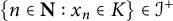
(see Corollary 3.3 below). It follows that
$\boldsymbol {y}$
(see Corollary 3.3 below). It follows that
However, by construction, we have that
 $y_ny_{n+1}<0$
whenever
$y_ny_{n+1}<0$
whenever
 $y_n\neq 0$
. Therefore,
$y_n\neq 0$
. Therefore,
, for all
 $n \in A$
. Considering that
$n \in A$
. Considering that
 $\mathcal {Z}$
is a translation invariant ideal, it follows that
$\mathcal {Z}$
is a translation invariant ideal, it follows that
 $\boldsymbol {y}$
is a bounded sequence such that
$\boldsymbol {y}$
is a bounded sequence such that
. We conclude by Lemma 3.1
(ii) below that the sequence
 $\boldsymbol {y}$
has a negative statistical cluster point, contradicting the standing hypothesis that
$\boldsymbol {y}$
has a negative statistical cluster point, contradicting the standing hypothesis that
 $\mathcal {I}\text {-}\liminf \boldsymbol {y}>0$
.
$\mathcal {I}\text {-}\liminf \boldsymbol {y}>0$
.
Hence,
 $\boldsymbol {x}$
is
$\boldsymbol {x}$
is
 $\mathcal {Z}$
-optimal. However, because the length of block
$\mathcal {Z}$
-optimal. However, because the length of block
 $B_k$
is odd for each
$B_k$
is odd for each
 $k\ge 2$
, it follows that
$k\ge 2$
, it follows that
 $\liminf \boldsymbol {x}=-1$
and
$\liminf \boldsymbol {x}=-1$
and
 $\limsup \boldsymbol {x}=1$
.
$\limsup \boldsymbol {x}=1$
.
With these premises, we give below a practical application of our main result in the context of (correspondences generated by) iterated function systems, a basic tool in fractal geometry (see, e.g., [Reference Falconer8]). Additional examples can be found also in [Reference Mammadov and Szuca22].
Example 2.6 Set
 $X=\mathbf {R}$
, let
$X=\mathbf {R}$
, let
 $\mathcal {I}$
be a translation invariant ideal on
$\mathcal {I}$
be a translation invariant ideal on
 $\mathbf {N}$
, and let
$\mathbf {N}$
, and let
 $u: \mathbf {R}\to \mathbf {R}$
be a strictly increasing continuous function. In addition, let
$u: \mathbf {R}\to \mathbf {R}$
be a strictly increasing continuous function. In addition, let
 $\{\phi _1,\ldots ,\phi _k\}$
be an iterated function system on
$\{\phi _1,\ldots ,\phi _k\}$
be an iterated function system on
 $\mathbf {R}$
, that is, a finite number of contractions on
$\mathbf {R}$
, that is, a finite number of contractions on
 $\mathbf {R}$
, and define the correspondence
$\mathbf {R}$
, and define the correspondence
 $\Phi : \mathbf {R}\rightrightarrows \mathbf {R}$
by
$\Phi : \mathbf {R}\rightrightarrows \mathbf {R}$
by
 $$ \begin{align*}\forall x \in \mathbf{R}, \quad \Phi(x):=\{\phi_1(x),\ldots,\phi_k(x)\}. \end{align*} $$
Accordingly, let
 $\mathscr {C}$
be an arbitrary subset of bounded feasible sequences such that
$\mathscr {C}$
be an arbitrary subset of bounded feasible sequences such that
 $$ \begin{align} \forall i=1,\ldots,k, \exists x \in \mathbf{R}, \quad (x, \phi_i(x), \phi_i^2(x),\ldots) \in \mathscr{C}. \end{align} $$
(It is remarkable that there exists a unique nonempty compact set
 $S\subseteq \mathbf {R}$
, called attractor, such that
$S\subseteq \mathbf {R}$
, called attractor, such that
 $\lim _n H^n(\{x_0\})=S$
, for all
$\lim _n H^n(\{x_0\})=S$
, for all
 $x_0 \in \mathbf {R}$
, in the Hausdorff metric, where H stands for Hutchinson operator defined by
$x_0 \in \mathbf {R}$
, in the Hausdorff metric, where H stands for Hutchinson operator defined by
 $H(A):= \bigcup _{x \in A}\Phi (x)$
, for all
$H(A):= \bigcup _{x \in A}\Phi (x)$
, for all
 $A\subseteq \mathbf {R}$
; see [Reference Hutchinson13].)
$A\subseteq \mathbf {R}$
; see [Reference Hutchinson13].)
For each
 $i=1,\ldots ,k$
, let
$i=1,\ldots ,k$
, let
 $\eta _i$
be the fixed point of
$\eta _i$
be the fixed point of
 $\phi _i$
, hence the restriction of u on
$\phi _i$
, hence the restriction of u on
 $\mathrm {Fix}(\Phi )=\{\eta _1,\ldots ,\eta _k\}$
is maximized at the unique point
$\mathrm {Fix}(\Phi )=\{\eta _1,\ldots ,\eta _k\}$
is maximized at the unique point
 $\eta ^\star =\max \{\eta _1,\ldots ,\eta _k\}$
. In particular, conditions (A1)–(A4) hold. At this point, note that
$\eta ^\star =\max \{\eta _1,\ldots ,\eta _k\}$
. In particular, conditions (A1)–(A4) hold. At this point, note that
 $F= [\eta ^\star , \infty )$
and
$F= [\eta ^\star , \infty )$
and
 $$ \begin{align*} \begin{aligned} \forall i=1,\ldots,k, \forall \eta>\eta_i, \quad \phi_i(\eta)-\eta_i \le |\phi_i(\eta)-\phi_i(\eta_i)|< \eta-\eta_i, \end{aligned} \end{align*} $$
hence
 $\phi _i(\eta )<\eta $
whenever
$\phi _i(\eta )<\eta $
whenever
 $\eta>\eta _i$
. In particular,
$\eta>\eta _i$
. In particular,
 $\max \Phi (\eta ^\star )=\eta ^\star $
and
$\max \Phi (\eta ^\star )=\eta ^\star $
and
 $\max \Phi (\eta )<\eta $
, for all
$\max \Phi (\eta )<\eta $
, for all
 $\eta>\eta ^\star $
. Therefore, condition (A5) holds letting T be the identity map. Finally, let j be an index such that
$\eta>\eta ^\star $
. Therefore, condition (A5) holds letting T be the identity map. Finally, let j be an index such that
 $\eta _{j}=\eta ^\star $
. Then, it follows by (2.4) and the Banach contraction theorem that there exists
$\eta _{j}=\eta ^\star $
. Then, it follows by (2.4) and the Banach contraction theorem that there exists
 $x \in \mathbf {R}$
such that
$x \in \mathbf {R}$
such that
 $(x, \phi _j(x), \phi _j^2(x), \ldots ) \in \mathscr {C}$
and
$(x, \phi _j(x), \phi _j^2(x), \ldots ) \in \mathscr {C}$
and
 $\lim _n \phi ^n_j(x)=\eta ^\star $
.
$\lim _n \phi ^n_j(x)=\eta ^\star $
.
We conclude by Corollary 2.2 that, if a sequence
 $\boldsymbol {x}$
in the constraint set
$\boldsymbol {x}$
in the constraint set
 $\mathscr {C}$
is
$\mathscr {C}$
is
 $\mathcal {I}$
-optimal, then
$\mathcal {I}$
-optimal, then
 $\mathcal {I}\text {-}\lim \boldsymbol {x}=\eta ^\star $
. In particular, in the special case
$\mathcal {I}\text {-}\lim \boldsymbol {x}=\eta ^\star $
. In particular, in the special case
 $\mathscr {C}=\mathscr {F}_{\mathrm {K}}$
,
$\mathscr {C}=\mathscr {F}_{\mathrm {K}}$
,
 $u(x)=x$
, and
$u(x)=x$
, and
 $\mathcal {I}=\mathrm {Fin}$
, we obtain that: if a bounded feasible sequence
$\mathcal {I}=\mathrm {Fin}$
, we obtain that: if a bounded feasible sequence
 $\boldsymbol {x}$
maximizes its smallest accumulation point, then it is convergent to the maximal fixed point
$\boldsymbol {x}$
maximizes its smallest accumulation point, then it is convergent to the maximal fixed point
 $\eta ^\star $
(this could be obtained, of course, also by a direct method.)
$\eta ^\star $
(this could be obtained, of course, also by a direct method.)
As a last motivation for the assumptions given in Theorem 2.1, we provide in Section 5 an example where our main result holds in an infinite dimensional vector space X (we postpone it because of its length). The proofs of our results are given in Section 4.
3 Preliminaries on
$\mathcal {I}$
-cluster points

We collect in the next lemma the basic properties of
 $\mathcal {I}$
-cluster points and
$\mathcal {I}$
-cluster points and
 $\mathcal {I}$
-convergence. These properties hold in greater generality, which we do not require here.
$\mathcal {I}$
-convergence. These properties hold in greater generality, which we do not require here.
Lemma 3.1 Let
 $\boldsymbol {x}$
be a sequence taking values in a metric space S and fix an ideal
$\boldsymbol {x}$
be a sequence taking values in a metric space S and fix an ideal
 $\mathcal {I}$
. Then:
$\mathcal {I}$
. Then:
-
(i)
$\Gamma _{\boldsymbol {x}}(\mathcal {I})$
is closed; -
(ii)
$\Gamma _{\boldsymbol {x}}(\mathcal {I})\cap K\neq \emptyset $
, provided that there exists a compact
$K\subseteq S$
such that
$\{n \in \mathbf {N}: x_n\in K\}\in \mathcal {I}^+$
; -
(iii)
$\mathcal {I}\text {-}\lim \boldsymbol {x}=\eta $
implies
$\Gamma _{\boldsymbol {x}}(\mathcal {I})=\{\eta \}$
; -
(iv)
$\mathcal {I}\text {-}\lim \boldsymbol {x}=\eta $
if and only if
$\Gamma _{\boldsymbol {x}}(\mathcal {I})=\{\eta \}$
, provided that there exists a compact
$K\subseteq S$
such that
$\{n \in \mathbf {N}: x_n \in K\} \in \mathcal {I}^\star $
; -
(v)
$\Gamma _{\boldsymbol {x}}(\mathcal {I})$
is the smallest closed set C such that
$\{n \in \mathbf {N}: x_n \in U\}\in \mathcal {I}^\star $
for all open sets
$U\supseteq C$
, provided that there exists a compact
$K\subseteq S$
such that
$\{n \in \mathbf {N}: x_n \in K\} \in \mathcal {I}^\star $
.


Proof See [Reference Leonetti and Maccheroni16, Lemma 3.1, Corollaries 3.2 and 3.4, and Theorem 4.3].▪
To the best of our knowledge, the following result is the first one of this type, even if some consequences were known (cf. Corollary 3.3 below). Informally, it states that, for each sequence contained in a compact, the set of
 $\mathcal {I}$
-cluster points of its continuous image coincides with the continuous image of its
$\mathcal {I}$
-cluster points of its continuous image coincides with the continuous image of its
 $\mathcal {I}$
-cluster points.
$\mathcal {I}$
-cluster points.
Proposition 3.2 Let
 $S,S^\prime $
be metric spaces, and let
$S,S^\prime $
be metric spaces, and let
 $\mathcal {I}$
be an ideal. Fix also a continuous function
$\mathcal {I}$
be an ideal. Fix also a continuous function
 $h:S\to S^\prime $
, and let
$h:S\to S^\prime $
, and let
 $\boldsymbol {x}$
be a sequence with values in S such that
$\boldsymbol {x}$
be a sequence with values in S such that
 $\{n \in \mathbf {N}: x_n \in K\} \in \mathcal {I}^\star $
for some compact
$\{n \in \mathbf {N}: x_n \in K\} \in \mathcal {I}^\star $
for some compact
 $K\subseteq S$
. Then,
$K\subseteq S$
. Then,
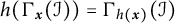 $h(\Gamma _{\boldsymbol {x}}(\mathcal {I}))=\Gamma _{h(\boldsymbol {x})}(\mathcal {I})$
.
$h(\Gamma _{\boldsymbol {x}}(\mathcal {I}))=\Gamma _{h(\boldsymbol {x})}(\mathcal {I})$
.
Proof First, suppose that
 $\eta \in \Gamma _{\boldsymbol {x}}(\mathcal {I})$
. Then, it follows by the continuity of h that
$\eta \in \Gamma _{\boldsymbol {x}}(\mathcal {I})$
. Then, it follows by the continuity of h that
 $h(\eta ) \in \Gamma _{h(\boldsymbol {x})}(\mathcal {I})$
: indeed, for each open neighborhood U of
$h(\eta ) \in \Gamma _{h(\boldsymbol {x})}(\mathcal {I})$
: indeed, for each open neighborhood U of
 $h(\eta )$
, there exists an open neighborhood V of
$h(\eta )$
, there exists an open neighborhood V of
 $\eta $
such that
$\eta $
such that
 $\{n \in \mathbf {N}: x_n \in V\} \subseteq \{n \in \mathbf {N}: h(x_n) \in U\}$
. Hence,
$\{n \in \mathbf {N}: x_n \in V\} \subseteq \{n \in \mathbf {N}: h(x_n) \in U\}$
. Hence,
 $h(\Gamma _{\boldsymbol {x}}(\mathcal {I}))\subseteq \Gamma _{h(\boldsymbol {x})}(\mathcal {I})$
.
$h(\Gamma _{\boldsymbol {x}}(\mathcal {I}))\subseteq \Gamma _{h(\boldsymbol {x})}(\mathcal {I})$
.
Conversely, suppose that
 $\nu \in \Gamma _{h(\boldsymbol {x})}(\mathcal {I})$
. Note that
$\nu \in \Gamma _{h(\boldsymbol {x})}(\mathcal {I})$
. Note that
 $F:=h^{-1}(\{\nu \})$
is closed and that
$F:=h^{-1}(\{\nu \})$
is closed and that
 $\{n \in \mathbf {N}: h(x_n) \in H\} \in \mathcal {I}^\star $
, where
$\{n \in \mathbf {N}: h(x_n) \in H\} \in \mathcal {I}^\star $
, where
 $H:=h(K)$
is compact. Because
$H:=h(K)$
is compact. Because
 $\nu $
belongs to H, then
$\nu $
belongs to H, then
 $K_0:=F \cap K$
is a nonempty compact set. We claim that there exists
$K_0:=F \cap K$
is a nonempty compact set. We claim that there exists
 $\eta \in K_0$
which is also an
$\eta \in K_0$
which is also an
 $\mathcal {I}$
-cluster point of
$\mathcal {I}$
-cluster point of
 $\boldsymbol {x}$
. To show this, for each
$\boldsymbol {x}$
. To show this, for each
 $r>0$
, let
$r>0$
, let
 $V_r$
be the closed ball with center
$V_r$
be the closed ball with center
 $\nu $
and radius r. Moreover, for each
$\nu $
and radius r. Moreover, for each
 $x \in F$
, let
$x \in F$
, let
 $U_{x,r}$
be the open ball with center x and radius r.
$U_{x,r}$
be the open ball with center x and radius r.
Because h is continuous and K is compact, then
 $G_r:=K\cap h^{-1}(V_r)$
is compact and contains
$G_r:=K\cap h^{-1}(V_r)$
is compact and contains
 $K_0$
for each
$K_0$
for each
 $r>0$
. Let
$r>0$
. Let
 $h_0$
be the restriction of h to the compact set K, so that
$h_0$
be the restriction of h to the compact set K, so that
 $h_0$
is uniformly continuous. It follows that
$h_0$
is uniformly continuous. It follows that
 $h_0$
admits a modulus of continuity, i.e., there exists a function
$h_0$
admits a modulus of continuity, i.e., there exists a function
 $\omega : [0,\infty ] \to [0,\infty ]$
such that
$\omega : [0,\infty ] \to [0,\infty ]$
such that
 $$ \begin{align*}\textstyle \lim_{r\to 0}\omega(r)=0 \,\,\,\,\,\text{ and }\,\,\,\,\, \forall a,b \in K, \quad d^\prime(h_0(a),h_0(b)) \le \omega (d(a,b)), \end{align*} $$
where d and
 $d^\prime $
represent the metric on S and
$d^\prime $
represent the metric on S and
 $S^\prime $
, respectively. In particular,
$S^\prime $
, respectively. In particular,
 $\omega $
is finite in a (right) neighborhood of
$\omega $
is finite in a (right) neighborhood of
 $0$
, let us say
$0$
, let us say
 $[0,\varepsilon ]$
. Replacing, if necessary, each
$[0,\varepsilon ]$
. Replacing, if necessary, each
 $\omega (r)$
with
$\omega (r)$
with
 $\sup _{q\le r}\omega (q)$
, we can assume without loss of generality that
$\sup _{q\le r}\omega (q)$
, we can assume without loss of generality that
 $\omega $
is nondecreasing. Finally, let
$\omega $
is nondecreasing. Finally, let
 $\omega ^{-1}$
be the generalized inverse of
$\omega ^{-1}$
be the generalized inverse of
 $\omega $
, i.e.,
$\omega $
, i.e.,
 $\omega ^{-1}(r):=\inf \{q: \omega (q)>r\}$
, for each
$\omega ^{-1}(r):=\inf \{q: \omega (q)>r\}$
, for each
 $r>0$
. For each
$r>0$
. For each
 $r>0$
, we obtain that
$r>0$
, we obtain that
 $ r\le \sup \omega (d(a,b)), $
where the supremum is taken with respect to all
$ r\le \sup \omega (d(a,b)), $
where the supremum is taken with respect to all
 $a \in F$
and
$a \in F$
and
 $b \in U_{a,\omega ^{-1}(r)}$
. This implies that
$b \in U_{a,\omega ^{-1}(r)}$
. This implies that
 $$ \begin{align} \textstyle \forall r>0, \quad G_{r}\subseteq \bigcup_{x \in F}U_{x,\, 2\omega^{-1}(r)}. \end{align} $$
However, because
 $G_r$
is compact, there exists
$G_r$
is compact, there exists
 $x_{r,1}, \ldots , x_{r, m_r} \in F$
such that
$x_{r,1}, \ldots , x_{r, m_r} \in F$
such that
 $G_r$
is contained into
$G_r$
is contained into
 $\bigcup _{i\le m_r}U_{x_{r,i}, 2\omega ^{-1}(r)}$
. To conclude, for each
$\bigcup _{i\le m_r}U_{x_{r,i}, 2\omega ^{-1}(r)}$
. To conclude, for each
 $r>0$
, we have that
$r>0$
, we have that
 $A_r:=\{n \in \mathbf {N}: h(x_n) \in V_r\} \in \mathcal {I}^+$
, hence it follows by (3.1) that
$A_r:=\{n \in \mathbf {N}: h(x_n) \in V_r\} \in \mathcal {I}^+$
, hence it follows by (3.1) that
 $$ \begin{align*}\textstyle A_r\backslash I=\{n \in \mathbf{N}: x_n \in G_r\}\subseteq \bigcup_{i\le m_r}\{n \in \mathbf{N}: x_n \in U_{x_{r,i}, 2\omega^{-1}(r)}\}, \end{align*} $$
where
 $I:=\{n \in \mathbf {N}: x_n \notin K\} \in \mathcal {I}$
. Because
$I:=\{n \in \mathbf {N}: x_n \notin K\} \in \mathcal {I}$
. Because
 $A_r\backslash I \in \mathcal {I}^+$
and
$A_r\backslash I \in \mathcal {I}^+$
and
 $\mathcal {I}$
is closed under finite unions, it follows that, for each
$\mathcal {I}$
is closed under finite unions, it follows that, for each
 $t \in \mathbf {N}$
, there exists
$t \in \mathbf {N}$
, there exists
 $k(t) \in \{1,\ldots ,m_{1/t}\}$
such that
$k(t) \in \{1,\ldots ,m_{1/t}\}$
such that
 $$ \begin{align*}B_t:=\{n \in \mathbf{N}: x_n \in U_{x_{1/t, k(t)}, 2\omega^{-1}(1/t)}\}\in \mathcal{I}^+. \end{align*} $$
Because
 $(x_{1/t, k(t)}: t \in \mathbf {N})$
is a sequence in the compact set
$(x_{1/t, k(t)}: t \in \mathbf {N})$
is a sequence in the compact set
 $K_0$
, there exists a convergent subsequence with limit, let us say,
$K_0$
, there exists a convergent subsequence with limit, let us say,
 $\eta \in K_0$
. Considering that
$\eta \in K_0$
. Considering that
 $\lim _t 2\omega ^{-1}(1/t)=0$
and that, for every
$\lim _t 2\omega ^{-1}(1/t)=0$
and that, for every
 $r>0$
, the set
$r>0$
, the set
 $C_r:=\{n \in \mathbf {N}: x_n \in U_{\eta ,r}\}$
contains
$C_r:=\{n \in \mathbf {N}: x_n \in U_{\eta ,r}\}$
contains
 $B_t$
for every t sufficiently large in the latter subsequence, we obtain that
$B_t$
for every t sufficiently large in the latter subsequence, we obtain that
 $C_r \in \mathcal {I}^+$
, for all
$C_r \in \mathcal {I}^+$
, for all
 $r>0$
. In other words,
$r>0$
. In other words,
 $\eta \in \Gamma _{\boldsymbol {x}}(\mathcal {I})$
and
$\eta \in \Gamma _{\boldsymbol {x}}(\mathcal {I})$
and
 $h(\eta )=\nu $
. This shows that
$h(\eta )=\nu $
. This shows that
 $\Gamma _{h(\boldsymbol {x})}(\mathcal {I})\subseteq h(\Gamma _{\boldsymbol {x}}(\mathcal {I}))$
, concluding the proof.▪
$\Gamma _{h(\boldsymbol {x})}(\mathcal {I})\subseteq h(\Gamma _{\boldsymbol {x}}(\mathcal {I}))$
, concluding the proof.▪
Corollary 3.3 Let S be a metric space and
 $\mathcal {I}$
be an ideal. In addition, fix a continuous function
$\mathcal {I}$
be an ideal. In addition, fix a continuous function
 $h: S\to \mathbf {R}$
and a sequence
$h: S\to \mathbf {R}$
and a sequence
 $\boldsymbol {x}$
in S such that
$\boldsymbol {x}$
in S such that
 $\{n \in \mathbf {N}: x_n \in K\} \in \mathcal {I}^\star $
for some compact
$\{n \in \mathbf {N}: x_n \in K\} \in \mathcal {I}^\star $
for some compact
 $K\subseteq S$
. Then,
$K\subseteq S$
. Then,
 $$ \begin{align} \textstyle \mathcal{I}\text{-}\liminf h(\boldsymbol{x})=\min \Gamma_{h(\boldsymbol{x})}(\mathcal{I})=\min_{\eta \in \Gamma_{\boldsymbol{x}}(\mathcal{I})}h(\eta), \end{align} $$
and, simmetrically,
 $$ \begin{align} \textstyle \mathcal{I}\text{-}\limsup h(\boldsymbol{x})=\max \Gamma_{h(\boldsymbol{x})}(\mathcal{I})=\max_{\eta \in \Gamma_{\boldsymbol{x}}(\mathcal{I})}h(\eta). \end{align} $$
Proof The first equality of (3.2) is a consequence of [Reference Leonetti15, Corollary 2.3] (cf. also [Reference Fridy and Orhan11, Theorem 1
 $^{\prime }$
] for the case
$^{\prime }$
] for the case
 $\mathcal {I}=\mathcal {Z}$
). The second equality of (3.2) follows directly by Proposition 3.2. The proof for the case
$\mathcal {I}=\mathcal {Z}$
). The second equality of (3.2) follows directly by Proposition 3.2. The proof for the case
 $S=\mathbf {R}^n$
and
$S=\mathbf {R}^n$
and
 $\mathcal {I}=\mathcal {Z}$
can be found also in [Reference Pehlivan and Mamedov25, Lemma 3.1].
$\mathcal {I}=\mathcal {Z}$
can be found also in [Reference Pehlivan and Mamedov25, Lemma 3.1].
The proof of (3.3) is analogous.▪
4 Proofs
Proof of Theorem 2.1
 $\quad $
Suppose that
$\quad $
Suppose that
 $\boldsymbol {x}$
is an
$\boldsymbol {x}$
is an
 $\mathcal {I}$
-optimal path. Because
$\mathcal {I}$
-optimal path. Because
 $\boldsymbol {x} \in \mathscr {C}\subseteq \mathscr {K}$
, there exists a compact set
$\boldsymbol {x} \in \mathscr {C}\subseteq \mathscr {K}$
, there exists a compact set
 $K\subseteq X$
such that
$K\subseteq X$
such that
 $\{n \in \mathbf {N}: x_n \notin K\} \in \mathcal {I}$
. It follows by (2.1), Corollary 3.3, and conditions (A2) and (A6) that
$\{n \in \mathbf {N}: x_n \notin K\} \in \mathcal {I}$
. It follows by (2.1), Corollary 3.3, and conditions (A2) and (A6) that
 $$ \begin{align*} \min_{\eta \in \Gamma_{\boldsymbol{x}}(\mathcal{I})} u(\eta) =\mathcal{I}\text{-}\liminf u(\boldsymbol{x}) \ge \sup_{\boldsymbol{y} \in \mathscr{C}}\mathcal{I}\text{-}\liminf u(\boldsymbol{y})\ge u(\eta^\star), \end{align*} $$
hence
 $\Gamma _{\boldsymbol {x}}(\mathcal {I})\subseteq K \cap F$
, where we recall that F is the closed set
$\Gamma _{\boldsymbol {x}}(\mathcal {I})\subseteq K \cap F$
, where we recall that F is the closed set
 $\{x \in X: u(x) \ge u(\eta ^\star )\}$
. Because K is compact and
$\{x \in X: u(x) \ge u(\eta ^\star )\}$
. Because K is compact and
 $\Gamma _{\boldsymbol {x}}(\mathcal {I})$
is closed by Lemma 3.1
(i), we obtain that
$\Gamma _{\boldsymbol {x}}(\mathcal {I})$
is closed by Lemma 3.1
(i), we obtain that
 $\Gamma _{\boldsymbol {x}}(\mathcal {I})$
is compact. In addition, it is nonempty by Lemma 3.1
(ii), therefore
$\Gamma _{\boldsymbol {x}}(\mathcal {I})$
is compact. In addition, it is nonempty by Lemma 3.1
(ii), therefore
 $\Gamma _{\boldsymbol {x}}(\mathcal {I})\in \mathcal {K}$
.
$\Gamma _{\boldsymbol {x}}(\mathcal {I})\in \mathcal {K}$
.
Suppose that
 $F=\{\eta ^\star \}$
. Because
$F=\{\eta ^\star \}$
. Because
 $\Gamma _{\boldsymbol {x}}(\mathcal {I})$
is a nonempty subset of F, it follows that
$\Gamma _{\boldsymbol {x}}(\mathcal {I})$
is a nonempty subset of F, it follows that
 $\Gamma _{\boldsymbol {x}}(\mathcal {I})=\{\eta ^\star \}$
, hence
$\Gamma _{\boldsymbol {x}}(\mathcal {I})=\{\eta ^\star \}$
, hence
 $\mathcal {I}\text {-}\lim \boldsymbol {x}=\eta ^\star $
by Lemma 3.1
(iv).
$\mathcal {I}\text {-}\lim \boldsymbol {x}=\eta ^\star $
by Lemma 3.1
(iv).
Let us suppose hereafter that
 $|F|\ge 2$
, so that the linear operator T in (A5) is nonzero. Replacing T with
$|F|\ge 2$
, so that the linear operator T in (A5) is nonzero. Replacing T with
 $T/\|T\|$
, we can assume without loss of generality that
$T/\|T\|$
, we can assume without loss of generality that
 $\|T\|=1$
.
$\|T\|=1$
.
Claim 1 The map
 $ \textstyle \mathrm {Gr}(\Phi )\to \mathbf {R}: (x,y) \mapsto T(x-y) $
is continuous.
$ \textstyle \mathrm {Gr}(\Phi )\to \mathbf {R}: (x,y) \mapsto T(x-y) $
is continuous.
Proof The claimed map can be rewritten as the restriction on
 $\mathrm {Gr}(\Phi )$
of the composition
$\mathrm {Gr}(\Phi )$
of the composition
 $T\circ g$
, where g is the continuous function
$T\circ g$
, where g is the continuous function
 $g: X^2\to X: (x,y) \mapsto x-y$
.▪
$g: X^2\to X: (x,y) \mapsto x-y$
.▪
Because T is continuous and
 $\Phi (x) \in \mathcal {K}$
, for each
$\Phi (x) \in \mathcal {K}$
, for each
 $x \in X$
, the function
$x \in X$
, the function
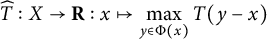 $$ \begin{align*} \widehat{T}: X\to \mathbf{R}: x\mapsto \max_{y \in \Phi(x)}T(y-x) \end{align*} $$
is well defined. Because the maximum is reached, we have
 $\widehat {T}x<0$
, for all
$\widehat {T}x<0$
, for all
 $x \in F\backslash \{\eta ^\star \}$
, by (A5).
$x \in F\backslash \{\eta ^\star \}$
, by (A5).
Claim 2
 $\widehat {T}$
is continuous and
$\widehat {T}$
is continuous and
 $\widehat {T}\eta ^\star =0$
.
$\widehat {T}\eta ^\star =0$
.
Proof Because
 $\Phi $
is a continuous correspondence by (A1) and the map defined in Claim 1 is continuous, it follows by Berge’s maximum theorem [Reference Aliprantis and Border1, Theorem 17.31] that
$\Phi $
is a continuous correspondence by (A1) and the map defined in Claim 1 is continuous, it follows by Berge’s maximum theorem [Reference Aliprantis and Border1, Theorem 17.31] that
 $\widehat {T}$
is continuous.
$\widehat {T}$
is continuous.
For the second part, we obtain by (A5) that
 $T(y-\eta ^\star )< 0$
, for all
$T(y-\eta ^\star )< 0$
, for all
 $y \in \Phi (\eta ^\star )$
, with
$y \in \Phi (\eta ^\star )$
, with
 $y\neq \eta ^\star $
. Because
$y\neq \eta ^\star $
. Because
 $\eta ^\star \in \mathrm {Fix}(\Phi )$
, we conclude that
$\eta ^\star \in \mathrm {Fix}(\Phi )$
, we conclude that
 $\widehat {T}\eta ^\star =T(\eta ^\star -\eta ^\star )=0$
.▪
$\widehat {T}\eta ^\star =T(\eta ^\star -\eta ^\star )=0$
.▪
Because T is continuous and
 $\boldsymbol {x} \in \mathscr {C} \subseteq \mathscr {K}$
, it follows that there exists
$\boldsymbol {x} \in \mathscr {C} \subseteq \mathscr {K}$
, it follows that there exists
 $M\in \mathbf {R}$
such that
$M\in \mathbf {R}$
such that
 $\{n \in \mathbf {N}: |Tx_n| \ge M\} \in \mathcal {I}$
. Hence, the
$\{n \in \mathbf {N}: |Tx_n| \ge M\} \in \mathcal {I}$
. Hence, the
 $\mathcal {I}$
-limit inferior and the
$\mathcal {I}$
-limit inferior and the
 $\mathcal {I}$
-limit superior of the real sequence
$\mathcal {I}$
-limit superior of the real sequence
 $(Tx_n)$
are well defined.
$(Tx_n)$
are well defined.
Claim 3 Fix
 $\eta \in \Gamma _{\boldsymbol {x}}(\mathcal {I})$
such that
$\eta \in \Gamma _{\boldsymbol {x}}(\mathcal {I})$
such that
 $\mathcal {I}\text {-}\liminf _n Tx_n=T\eta $
. Then,
$\mathcal {I}\text {-}\liminf _n Tx_n=T\eta $
. Then,
 $\eta =\eta ^\star $
.
$\eta =\eta ^\star $
.
Proof Assume that there exists
 $\eta _0 \in \Gamma _{\boldsymbol {x}}(\mathcal {I})$
different from
$\eta _0 \in \Gamma _{\boldsymbol {x}}(\mathcal {I})$
different from
 $\eta ^\star $
such that
$\eta ^\star $
such that
 $\mathcal {I}\text {-}\liminf _n Tx_n=T\eta _0$
. Because
$\mathcal {I}\text {-}\liminf _n Tx_n=T\eta _0$
. Because
 $\Gamma _{\boldsymbol {x}}(\mathcal {I})\subseteq F$
and
$\Gamma _{\boldsymbol {x}}(\mathcal {I})\subseteq F$
and
 $\eta _0\neq \eta ^\star $
, then
$\eta _0\neq \eta ^\star $
, then
 $\widehat {T}\eta _0<0$
. Because
$\widehat {T}\eta _0<0$
. Because
 $\widehat {T}$
is continuous by Claim 2, there exist
$\widehat {T}$
is continuous by Claim 2, there exist
 $\varepsilon ,\delta>0$
such that
$\varepsilon ,\delta>0$
such that
 $\widehat {T}x<-\varepsilon $
whenever
$\widehat {T}x<-\varepsilon $
whenever
 $\|x-\eta _0\|<\delta $
. Moreover, it can be assumed without loss of generality that
$\|x-\eta _0\|<\delta $
. Moreover, it can be assumed without loss of generality that
. At this point, fix
 $x,y \in X$
such that
$x,y \in X$
such that
 $\|x-\eta _0\|<\delta $
and
$\|x-\eta _0\|<\delta $
and
 $y \in \Phi (x)$
, and let
$y \in \Phi (x)$
, and let
 $\pi _{y}$
be a minimizer of
$\pi _{y}$
be a minimizer of
 $\|\pi -y\|$
with
$\|\pi -y\|$
with
 $\pi \in \Gamma _{\boldsymbol {x}}(\mathcal {I})$
. Because
$\pi \in \Gamma _{\boldsymbol {x}}(\mathcal {I})$
. Because
 $\widehat {T}x<-\varepsilon $
, we get
$\widehat {T}x<-\varepsilon $
, we get
At the same time, we have
 $$ \begin{align*}\textstyle Ty=T\pi_y+T(y-\pi_y)\ge T\eta_0-\|y-\pi_y\|, \end{align*} $$
which implies that
.
To sum up, if
 $\|x-\eta _0\|<\delta $
, then
$\|x-\eta _0\|<\delta $
, then
![]() , for all
, for all
 $y \in \Phi (x)$
. Because
$y \in \Phi (x)$
. Because
 $\eta _0$
is an
$\eta _0$
is an
 $\mathcal {I}$
-cluster point of
$\mathcal {I}$
-cluster point of
 $\boldsymbol {x}$
, we have
$\boldsymbol {x}$
, we have
 $A:=\{n \in \mathbf {N}: \|x_n-\eta _0\|<\delta \} \in \mathcal {I}^+$
. Thus, because
$A:=\{n \in \mathbf {N}: \|x_n-\eta _0\|<\delta \} \in \mathcal {I}^+$
. Thus, because
 $\mathcal {I}$
is translation invariant by (A3), then also
$\mathcal {I}$
is translation invariant by (A3), then also
 $A+1 \in \mathcal {I}^+$
. However, considering that
$A+1 \in \mathcal {I}^+$
. However, considering that
 $x_{n+1} \in \Phi (x_n)$
, for all
$x_{n+1} \in \Phi (x_n)$
, for all
 $n \in A$
, we obtain by the preceding part that
$n \in A$
, we obtain by the preceding part that
![]() . To sum up, the open set
. To sum up, the open set
![]() contains
contains
 $\Gamma _{\boldsymbol {x}}(\mathcal {I})$
and it has empty intersection with the
$\Gamma _{\boldsymbol {x}}(\mathcal {I})$
and it has empty intersection with the
 $\mathcal {I}$
-positive set
$\mathcal {I}$
-positive set
 $A+1$
. This contradicts Lemma 3.1
(v).▪
$A+1$
. This contradicts Lemma 3.1
(v).▪
Claim 4 Fix
 $\eta \in \Gamma _{\boldsymbol {x}}(\mathcal {I})$
such that
$\eta \in \Gamma _{\boldsymbol {x}}(\mathcal {I})$
such that
 $\mathcal {I}\text {-}\limsup _n Tx_n=T\eta $
. Then,
$\mathcal {I}\text {-}\limsup _n Tx_n=T\eta $
. Then,
 $T\eta =T\eta ^\star $
.
$T\eta =T\eta ^\star $
.
Proof Assume that there exists
 $\eta _0 \in \Gamma _{\boldsymbol {x}}(\mathcal {I})$
such that
$\eta _0 \in \Gamma _{\boldsymbol {x}}(\mathcal {I})$
such that
 $\mathcal {I}\text {-}\limsup _n Tx_n=T\eta $
and
$\mathcal {I}\text {-}\limsup _n Tx_n=T\eta $
and
 $T\eta \neq T\eta ^\star $
. Because
$T\eta \neq T\eta ^\star $
. Because
 $\eta ^\star $
is a minimizer of
$\eta ^\star $
is a minimizer of
 $T\eta $
with
$T\eta $
with
 $\eta \in \Gamma _{\boldsymbol {x}}(\mathcal {I})$
by Claim 3, then
$\eta \in \Gamma _{\boldsymbol {x}}(\mathcal {I})$
by Claim 3, then
 $\kappa :=T(\eta _0-\eta ^\star )>0$
.
$\kappa :=T(\eta _0-\eta ^\star )>0$
.
Because
 $\widehat {T}$
is continuous and
$\widehat {T}$
is continuous and
 $\widehat {T}\eta ^\star =0$
by Claim 2, there exist
$\widehat {T}\eta ^\star =0$
by Claim 2, there exist
such that
 $\widehat {T}x<\varepsilon $
whenever
$\widehat {T}x<\varepsilon $
whenever
 $\|x-\eta ^\star \|<\delta $
. Therefore, for each
$\|x-\eta ^\star \|<\delta $
. Therefore, for each
 $y \in \Phi (x)$
such that
$y \in \Phi (x)$
such that
 $\|x-\eta ^\star \|<\delta $
, we obtain
$\|x-\eta ^\star \|<\delta $
, we obtain
and, at the same time,
 $$ \begin{align*}Ty=T\eta_0+T(y-\eta_0) \ge T\eta^\star+\kappa-\|y-\eta_0\|. \end{align*} $$
Therefore,
whenever
 $\|x-\eta ^\star \|<\delta $
and
$\|x-\eta ^\star \|<\delta $
and
 $y \in \Phi (x)$
. It follows that, if
$y \in \Phi (x)$
. It follows that, if
 $x\in X$
is chosen such that
$x\in X$
is chosen such that
and
, for some
 $\eta \in \Gamma _{\boldsymbol {x}}(\mathcal {I})$
, then
$\eta \in \Gamma _{\boldsymbol {x}}(\mathcal {I})$
, then
 $\|x-\eta ^\star \|\le \|x-\eta \|+\|\eta -\eta ^\star \|<\delta $
and hence
$\|x-\eta ^\star \|\le \|x-\eta \|+\|\eta -\eta ^\star \|<\delta $
and hence
 $\|y-\eta _0\|<\kappa $
, for all
$\|y-\eta _0\|<\kappa $
, for all
 $y \in \Phi (x)$
.
$y \in \Phi (x)$
.
At this point, note that the set
is compact. Suppose that
 $Q\neq \emptyset $
. By the continuity of
$Q\neq \emptyset $
. By the continuity of
 $\widehat {T}$
, we have
$\widehat {T}$
, we have
 $\max _{\eta \in Q}\widehat {T}\eta <0$
. It follows there exist
$\max _{\eta \in Q}\widehat {T}\eta <0$
. It follows there exist
 $\lambda ,\tau>0$
such that
$\lambda ,\tau>0$
such that
 $\widehat {T}x<-\lambda $
whenever
$\widehat {T}x<-\lambda $
whenever
 $\|x-\eta \|<\tau $
, for some
$\|x-\eta \|<\tau $
, for some
 $\eta \in Q$
. In addition, it can be assumed without loss of generality that
$\eta \in Q$
. In addition, it can be assumed without loss of generality that
. Now, let us suppose that
 $x\in X$
is chosen such that
$x\in X$
is chosen such that
 $\|x-\eta \|<\tau $
for some fixed
$\|x-\eta \|<\tau $
for some fixed
 $\eta \in Q$
. Fix
$\eta \in Q$
. Fix
 $y \in \Phi (x)$
; then,
$y \in \Phi (x)$
; then,
so that
.
Set
![]() and fix
and fix
 $x,y \in X$
with
$x,y \in X$
with
 $y \in \Phi (x)$
. To sum up the previous observations, we have that:
$y \in \Phi (x)$
. To sum up the previous observations, we have that:
-
(i) If there exists
$\eta \in \Gamma _{\boldsymbol {x}}(\mathcal {I})$
such that
$\|x-\eta \|<\nu $
and
, then
$\|y-\eta _0\|>\nu $
; -
(ii) If there exists
$\eta \in \Gamma _{\boldsymbol {x}}(\mathcal {I})$
such that
$\|x-\eta \|<\nu $
and
(so that
$Q\neq \emptyset $
), then
$\|y-\eta _0\|>\nu $
.


Putting everything together, if
 $\|y-\eta _0\|\le \nu $
, then
$\|y-\eta _0\|\le \nu $
, then
 $\|x-\eta \|>\nu $
, for all
$\|x-\eta \|>\nu $
, for all
 $\eta \in \Gamma _{\boldsymbol {x}}(\mathcal {I})$
.
$\eta \in \Gamma _{\boldsymbol {x}}(\mathcal {I})$
.
We conclude as in the proof of Claim 3: because
 $A:=\{n \in \mathbf {N}: \|x_{n+1}-\eta _0\|\le \nu \} \in \mathcal {I}^+$
and
$A:=\{n \in \mathbf {N}: \|x_{n+1}-\eta _0\|\le \nu \} \in \mathcal {I}^+$
and
 $\mathcal {I}$
is translation invariant by (A3), then
$\mathcal {I}$
is translation invariant by (A3), then
 $A-1\in \mathcal {I}^+$
. However,
$A-1\in \mathcal {I}^+$
. However,
 $A-1$
is a subset of
$A-1$
is a subset of
 $\{n \in \mathbf {N}: \forall \eta \in \Gamma _{\boldsymbol {x}}(\mathcal {I}), \|x_n-\eta \|>\nu \}$
, which belongs to
$\{n \in \mathbf {N}: \forall \eta \in \Gamma _{\boldsymbol {x}}(\mathcal {I}), \|x_n-\eta \|>\nu \}$
, which belongs to
 $\mathcal {I}$
thanks to Lemma 3.1
(v). This contradiction concludes the proof.▪
$\mathcal {I}$
thanks to Lemma 3.1
(v). This contradiction concludes the proof.▪
To complete the proof, note that by Corollary 3.3 there exist nonempty compact sets
 $\Gamma _{\mathrm {min}}, \Gamma _{\mathrm {max}}\subseteq \Gamma _{\boldsymbol {x}}(\mathcal {I})$
such that
$\Gamma _{\mathrm {min}}, \Gamma _{\mathrm {max}}\subseteq \Gamma _{\boldsymbol {x}}(\mathcal {I})$
such that
 $\mathcal {I}\text {-}\liminf _n Tx_n=T\eta $
, for all
$\mathcal {I}\text {-}\liminf _n Tx_n=T\eta $
, for all
 $\eta \in \Gamma _{\mathrm {min}}$
, and
$\eta \in \Gamma _{\mathrm {min}}$
, and
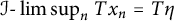 $\mathcal {I}\text {-}\limsup _n Tx_n=T\eta $
, for all
$\mathcal {I}\text {-}\limsup _n Tx_n=T\eta $
, for all
 $\eta \in \Gamma _{\mathrm {max}}$
. Hence, Claims 3 and 4 imply that
$\eta \in \Gamma _{\mathrm {max}}$
. Hence, Claims 3 and 4 imply that
 $$ \begin{align*}\{\eta^\star\}=\Gamma_{\mathrm{min}} \quad \text{ and }\quad \eta^\star \in \Gamma_{\mathrm{min}}\cap \Gamma_{\mathrm{max}}. \end{align*} $$
In other words, the function
 $\Gamma _{\boldsymbol {x}}(\mathcal {I})\to \mathbf {R}$
defined by
$\Gamma _{\boldsymbol {x}}(\mathcal {I})\to \mathbf {R}$
defined by
 $\eta \mapsto T\eta $
has a unique point of minimum which is also a maximizer. Therefore,
$\eta \mapsto T\eta $
has a unique point of minimum which is also a maximizer. Therefore,
 $\Gamma _{\boldsymbol {x}}(\mathcal {I})=\{\eta ^\star \}$
, which is equivalent to
$\Gamma _{\boldsymbol {x}}(\mathcal {I})=\{\eta ^\star \}$
, which is equivalent to
 $\mathcal {I}\text {-}\lim \boldsymbol {x}=\eta ^\star $
by Lemma 3.1
(iv).
$\mathcal {I}\text {-}\lim \boldsymbol {x}=\eta ^\star $
by Lemma 3.1
(iv).
 $\blacksquare $
Remark 4.1 As it is evident from the proof of Theorem 2.1, the full strength of condition (A5) has not been used. Indeed, we needed it only in Claim 3 to show that
 $\widehat {T}\eta _0<0$
for some
$\widehat {T}\eta _0<0$
for some
 $\eta _0 \in \Gamma _{\boldsymbol {x}}(\mathcal {I})$
and in Claim 4 to show that
$\eta _0 \in \Gamma _{\boldsymbol {x}}(\mathcal {I})$
and in Claim 4 to show that
 $\max _{\eta \in Q}\widehat {T}\eta <0$
for a suitable subset
$\max _{\eta \in Q}\widehat {T}\eta <0$
for a suitable subset
 $Q\subseteq \Gamma _{\boldsymbol {x}}(\mathcal {I})$
. Therefore, it is enough to replace (2.2) with the weaker condition
$Q\subseteq \Gamma _{\boldsymbol {x}}(\mathcal {I})$
. Therefore, it is enough to replace (2.2) with the weaker condition
 $$ \begin{align*}\forall x \in \Gamma_{\boldsymbol{x}}(\mathcal{I}), \forall y \in \Phi(x), \quad Tx \le Ty \implies x=y=\eta^\star. \end{align*} $$
However, this condition, differently from (A5), depends on a given sequence
 $\boldsymbol {x}$
.
$\boldsymbol {x}$
.
Proof of Corollary 2.2 Thanks to Theorem 2.1, it is sufficient to show that the existence of a sequence
 $\boldsymbol {y} \in \mathscr {C}$
which is
$\boldsymbol {y} \in \mathscr {C}$
which is
 $\mathcal {I}$
-convergent to
$\mathcal {I}$
-convergent to
 $\eta ^\star $
implies condition (A6). To this aim, observe that
$\eta ^\star $
implies condition (A6). To this aim, observe that
 $\Gamma _{\boldsymbol {y}}(\mathcal {I})=\{\eta ^\star \}$
by Lemma 3.1
(iii). It follows by Corollary 3.3 that
$\Gamma _{\boldsymbol {y}}(\mathcal {I})=\{\eta ^\star \}$
by Lemma 3.1
(iii). It follows by Corollary 3.3 that
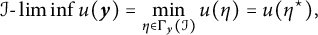 $$ \begin{align*} \mathcal{I}\text{-}\liminf u(\boldsymbol{y}) =\min_{\eta \in \Gamma_{\boldsymbol{y}}(\mathcal{I})} u(\eta) = u(\eta^\star), \end{align*} $$
concluding the proof.▪
Proof of Corollary 2.4 It is enough to note that every
 $\mathcal {I}$
-cluster point is an ordinary accumulation point, so that by Corollary 3.3 we obtain
$\mathcal {I}$
-cluster point is an ordinary accumulation point, so that by Corollary 3.3 we obtain
 $$ \begin{align*} \begin{aligned} \textstyle \sup_{y \in C}\mathcal{I}\text{-}\liminf_n u(\phi^n(y)) &\textstyle \ge \mathcal{I}\text{-}\liminf_n u(\phi^n(y_0))\\ &\textstyle =\min \Gamma_{(u(\phi^n(y_0)))}(\mathcal{I}) \ge \liminf_n u(\phi^n(y_0))\ge u(\eta^\star). \end{aligned} \end{align*} $$
Hence, condition (A6) holds, and the conclusion follows by Theorem 2.1.▪
5 An infinite dimensional example
As promised, we provide a practical example where Theorem 2.1 holds in infinite dimension.
Example 5.1 Let X be the Hilbert space
 $\ell _2$
of square summable real sequences, i.e., sequences
$\ell _2$
of square summable real sequences, i.e., sequences
 $\boldsymbol {x}=(x_0,x_1,\ldots )$
such that
$\boldsymbol {x}=(x_0,x_1,\ldots )$
such that
 $$ \begin{align*}\textstyle \|\boldsymbol{x}\|:=\sqrt{\sum_{i\ge 0}x_i^2}<\infty. \end{align*} $$
Fix a sequence
 $\boldsymbol {x}^\star \in \ell _2$
, and define
$\boldsymbol {x}^\star \in \ell _2$
, and define
 $\mathscr {C}=\{(\boldsymbol {x}^{(n)}) \in \mathscr {F}_{\mathrm {K}}: \boldsymbol {x}^{(0)}=\boldsymbol {x}^\star \}$
. Let also
$\mathscr {C}=\{(\boldsymbol {x}^{(n)}) \in \mathscr {F}_{\mathrm {K}}: \boldsymbol {x}^{(0)}=\boldsymbol {x}^\star \}$
. Let also
 $\mathcal {I}$
be an arbitrary translation invariant ideal, and, for each
$\mathcal {I}$
be an arbitrary translation invariant ideal, and, for each
 $\boldsymbol {x} \in \ell _2$
, set
$\boldsymbol {x} \in \ell _2$
, set
 $u(\boldsymbol {x})=x_0$
and
$u(\boldsymbol {x})=x_0$
and
where
![]() . First of all, let us show that
. First of all, let us show that
 $\Phi $
is well defined. To do this, fix
$\Phi $
is well defined. To do this, fix
 $\boldsymbol {x} \in \ell _2$
and let us prove that
$\boldsymbol {x} \in \ell _2$
and let us prove that
 $\Phi (\boldsymbol {x})\subseteq \ell _2$
. If
$\Phi (\boldsymbol {x})\subseteq \ell _2$
. If
 $\boldsymbol {y} \in \Phi (\boldsymbol {x})$
is equal to
$\boldsymbol {y} \in \Phi (\boldsymbol {x})$
is equal to
 $\frac {1}{2}\boldsymbol {x}$
, then it clearly belongs to
$\frac {1}{2}\boldsymbol {x}$
, then it clearly belongs to
 $\ell _2$
. Otherwise, because
$\ell _2$
. Otherwise, because
 $\ell _2$
is a vector space, it is sufficient to show that
$\ell _2$
is a vector space, it is sufficient to show that
 $\boldsymbol {z}=\boldsymbol {y}-\boldsymbol {x}=(-x_0-\sum _{i\ge 1}x_i^2,z_1,z_2,\ldots ) \in \ell _2$
, where
$\boldsymbol {z}=\boldsymbol {y}-\boldsymbol {x}=(-x_0-\sum _{i\ge 1}x_i^2,z_1,z_2,\ldots ) \in \ell _2$
, where
![]() , for all
, for all
 $i\ge 1$
. Therefore,
$i\ge 1$
. Therefore,
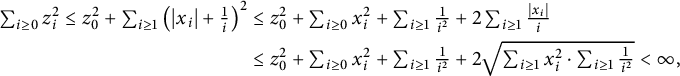 $$ \begin{align*} \begin{aligned} \textstyle \sum_{i\ge 0}z_i^2\le z_0^2+\sum_{i\ge 1}\left(|x_i|+\frac{1}{i}\right)^2 &\textstyle \le z_0^2+\sum_{i\ge 0}x_i^2+\sum_{i\ge 1}\frac{1}{i^2}+2\sum_{i\ge 1}\frac{|x_i|}{i} \\ &\textstyle \le z_0^2+\sum_{i\ge 0}x_i^2+\sum_{i\ge 1}\frac{1}{i^2}+2\sqrt{\sum_{i\ge 1}x_i^2 \cdot \sum_{i\ge 1}\frac{1}{i^2}}<\infty, \end{aligned} \end{align*} $$
where the last
 $\le $
follows by the Cauchy–Schwarz inequality. In addition,
$\le $
follows by the Cauchy–Schwarz inequality. In addition,
 $\Phi (\boldsymbol {x})$
is compact. To this aim, because
$\Phi (\boldsymbol {x})$
is compact. To this aim, because
 $\{\frac {1}{2}\boldsymbol {x}\}$
is compact, it is sufficient to show that a translation of the first set in the definition (5.1) of
$\{\frac {1}{2}\boldsymbol {x}\}$
is compact, it is sufficient to show that a translation of the first set in the definition (5.1) of
 $\Phi (\boldsymbol {x})$
is compact. Let us define
$\Phi (\boldsymbol {x})$
is compact. Let us define
Let
 $\boldsymbol {a}$
be the sequence defined by
$\boldsymbol {a}$
be the sequence defined by
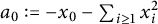 ${a}_0:=-x_0-\sum _{i\ge 1}x_i^2$
and
${a}_0:=-x_0-\sum _{i\ge 1}x_i^2$
and
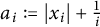 ${a}_i:=|x_i|+\frac {1}{i}$
. Note that
${a}_i:=|x_i|+\frac {1}{i}$
. Note that
 $\boldsymbol {a} \in \ell _2$
and that
$\boldsymbol {a} \in \ell _2$
and that
 $\varphi (\boldsymbol {x})$
is a closed subset of
$\varphi (\boldsymbol {x})$
is a closed subset of
 $\{\boldsymbol {z} \in \ell _2: |z_i| \le {a}_i \text { for all }i\ge 0\}$
. However, the latter set is compact thanks to [Reference Dunford and Schwartz7, p. 453], hence
$\{\boldsymbol {z} \in \ell _2: |z_i| \le {a}_i \text { for all }i\ge 0\}$
. However, the latter set is compact thanks to [Reference Dunford and Schwartz7, p. 453], hence
 $\varphi (\boldsymbol {x})$
is compact too. To sum up,
$\varphi (\boldsymbol {x})$
is compact too. To sum up,
 $\Phi (\boldsymbol {x})$
is compact subset of
$\Phi (\boldsymbol {x})$
is compact subset of
 $\ell _2$
which is nonempty (because it contains
$\ell _2$
which is nonempty (because it contains
 $\frac {1}{2}\boldsymbol {x}$
).
$\frac {1}{2}\boldsymbol {x}$
).
At this point, let us show that
 $\Phi $
is continuous. Reasoning as above, it is sufficient to show that the correspondence
$\Phi $
is continuous. Reasoning as above, it is sufficient to show that the correspondence
 $\varphi $
defined in (5.2) is continuous at
$\varphi $
defined in (5.2) is continuous at
 $\boldsymbol {x}$
. Assume that
$\boldsymbol {x}$
. Assume that
 $\varphi (\boldsymbol {x})\neq \emptyset $
, i.e.,
$\varphi (\boldsymbol {x})\neq \emptyset $
, i.e.,
![]() , for all
, for all
 $i\ge 1$
, otherwise the claim is trivial.
$i\ge 1$
, otherwise the claim is trivial.
First, let us show that
 $\varphi $
is upper hemicontinuous. Fix
$\varphi $
is upper hemicontinuous. Fix
 $\varepsilon>0$
and define the open set
$\varepsilon>0$
and define the open set
 $U_\varepsilon :=\{\boldsymbol {z} \in \ell _2: \exists \boldsymbol {y} \in \varphi (\boldsymbol {x}), \|\boldsymbol {z}-\boldsymbol {y}\|<\varepsilon \}$
. We need to find a constant
$U_\varepsilon :=\{\boldsymbol {z} \in \ell _2: \exists \boldsymbol {y} \in \varphi (\boldsymbol {x}), \|\boldsymbol {z}-\boldsymbol {y}\|<\varepsilon \}$
. We need to find a constant
 $\delta>0$
such that, for each
$\delta>0$
such that, for each
 $\boldsymbol {x}^\prime \in \ell _2$
, if
$\boldsymbol {x}^\prime \in \ell _2$
, if
 $\|\boldsymbol {x}-\boldsymbol {x}^\prime \|<\delta $
, then
$\|\boldsymbol {x}-\boldsymbol {x}^\prime \|<\delta $
, then
 $\varphi (\boldsymbol {x}^\prime ) \subseteq U_\varepsilon $
. Hence, fix also
$\varphi (\boldsymbol {x}^\prime ) \subseteq U_\varepsilon $
. Hence, fix also
 $\boldsymbol {x}^\prime \in \ell _2$
such that
$\boldsymbol {x}^\prime \in \ell _2$
such that
 $\|\boldsymbol {x}-\boldsymbol {x}^\prime \|<\delta $
for a suitable
$\|\boldsymbol {x}-\boldsymbol {x}^\prime \|<\delta $
for a suitable
 $\delta>0$
that will be chosen later and pick
$\delta>0$
that will be chosen later and pick
 $\boldsymbol {y}^\prime \in \varphi (\boldsymbol {x}^\prime )$
. In particular,
$\boldsymbol {y}^\prime \in \varphi (\boldsymbol {x}^\prime )$
. In particular,
 $|x_i-x_i^\prime |<\delta $
, for all
$|x_i-x_i^\prime |<\delta $
, for all
 $i \ge 0$
. Similarly, we can assume without loss of generality that
$i \ge 0$
. Similarly, we can assume without loss of generality that
![]() , for all
, for all
 $i\ge 1$
, otherwise
$i\ge 1$
, otherwise
 $\varphi (\boldsymbol {x}^\prime )=\emptyset $
. Then,
$\varphi (\boldsymbol {x}^\prime )=\emptyset $
. Then,
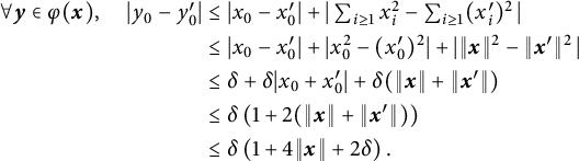 $$ \begin{align} \begin{aligned} \textstyle \forall \boldsymbol{y} \in \varphi(\boldsymbol{x}), \quad |y_0-y_0^\prime| &\textstyle \le |x_0-x_0^\prime|+|\sum_{i\ge 1}x_i^2-\sum_{i\ge 1}(x_i^\prime)^2\,|\\ &\textstyle \le |x_0-x_0^\prime|+|x_0^2-(x_0^\prime)^2|+|\|\boldsymbol{x}\|^2-\|\boldsymbol{x}^\prime\|^2\,| \\ &\textstyle \le \delta+\delta |x_0+x_0^\prime|+\delta(\|\boldsymbol{x}\|+\|\boldsymbol{x}^\prime\|) \\ &\textstyle \le \delta\left(1+2 (\|\boldsymbol{x}\|+\|\boldsymbol{x}^\prime\|)\right) \\ &\textstyle \le \delta\left(1+4\|\boldsymbol{x}\|+2\delta\right). \end{aligned} \end{align} $$
Now, recall that, for each integer
 $i\ge 1$
, we have
$i\ge 1$
, we have
![]() and
and
![]() . In particular, there exists
. In particular, there exists
 $\boldsymbol {y} \in \varphi (\boldsymbol {x})$
such that
$\boldsymbol {y} \in \varphi (\boldsymbol {x})$
such that
 $|y_i-y_i^\prime |\le |x_i-x_i^\prime |$
, for all
$|y_i-y_i^\prime |\le |x_i-x_i^\prime |$
, for all
 $i\ge 1$
. It follows that
$i\ge 1$
. It follows that
 $$ \begin{align} \textstyle \sum_{i\ge 1}(y_i-y_i^\prime)^2\le \sum_{i\ge 1}(x_i-x_i^\prime)^2 \le \|\boldsymbol{x}-\boldsymbol{x}^\prime\|^2 \le \delta^2. \end{align} $$
Putting together the above estimates, we obtain that, for each given
 $\boldsymbol {y}^\prime \in \varphi (\boldsymbol {x}^\prime )$
, there exists
$\boldsymbol {y}^\prime \in \varphi (\boldsymbol {x}^\prime )$
, there exists
 $\boldsymbol {y} \in \varphi (\boldsymbol {x})$
such that
$\boldsymbol {y} \in \varphi (\boldsymbol {x})$
such that
 $$ \begin{align} \textstyle \|\boldsymbol{y}-\boldsymbol{y}^\prime\|=\sqrt{|y_0-y_0^\prime|^2+\sum_{i\ge 1}(y_i-y_i^\prime)^2}\le \delta \sqrt{\left(1+4\|\boldsymbol{x}\|+2\delta\right)^2+1}<\varepsilon, \end{align} $$
where the last inequality holds if
 $\delta $
is sufficiently small.
$\delta $
is sufficiently small.
Second, let us show that
 $\varphi $
is lower hemicontinuous. To this aim, fix an arbitrary
$\varphi $
is lower hemicontinuous. To this aim, fix an arbitrary
 $\boldsymbol {y} \in \varphi (\boldsymbol {x})$
and some
$\boldsymbol {y} \in \varphi (\boldsymbol {x})$
and some
 $\varepsilon>0$
. We claim that there exists
$\varepsilon>0$
. We claim that there exists
 $\delta>0$
such that if
$\delta>0$
such that if
 $\|\boldsymbol {x}-\boldsymbol {x}^\prime \|<\delta $
, then
$\|\boldsymbol {x}-\boldsymbol {x}^\prime \|<\delta $
, then
 $\|\boldsymbol {y}-\boldsymbol {y}^\prime \|<\varepsilon $
, for some
$\|\boldsymbol {y}-\boldsymbol {y}^\prime \|<\varepsilon $
, for some
 $\boldsymbol {y}^\prime \in \varphi (\boldsymbol {x}^\prime )$
. Note that estimates (5.3) and (5.4) hold simmetrically also in this case, with the conclusion that we have exactly the same upper bound computed in (5.5) for
$\boldsymbol {y}^\prime \in \varphi (\boldsymbol {x}^\prime )$
. Note that estimates (5.3) and (5.4) hold simmetrically also in this case, with the conclusion that we have exactly the same upper bound computed in (5.5) for
 $\|\boldsymbol {y}-\boldsymbol {y}^\prime \|$
.
$\|\boldsymbol {y}-\boldsymbol {y}^\prime \|$
.
Therefore,
 $\Phi $
is a nonempty compact-valued continuous correspondence on
$\Phi $
is a nonempty compact-valued continuous correspondence on
 $\ell _2$
,
$\ell _2$
,
 $\mathcal {I}$
is translation invariant, and u is clearly continuous. Hence, conditions (A1)–(A3) hold.
$\mathcal {I}$
is translation invariant, and u is clearly continuous. Hence, conditions (A1)–(A3) hold.
The set of fixed points of
 $\Phi $
is neither convex nor compact, and it is equal to
$\Phi $
is neither convex nor compact, and it is equal to
 $$ \begin{align*}\textstyle \mathrm{Fix}(\Phi)=\{\boldsymbol{x} \in \ell_2: x_0=-\sum_{i\ge 1}x_i^2 \text{ and }x_j\le 0 \text{ for all }j\ge 1\}. \end{align*} $$
It follows that the restriction of u on
 $\mathrm {Fix}(\Phi )$
has a unique maximizer, which is the zero sequence
$\mathrm {Fix}(\Phi )$
has a unique maximizer, which is the zero sequence
 $\boldsymbol {0}$
of
$\boldsymbol {0}$
of
 $\ell _2$
, hence condition (A4) holds. Moreover, we have that
$\ell _2$
, hence condition (A4) holds. Moreover, we have that
 $$ \begin{align*}F=\{\boldsymbol{x} \in \mathscr{C}: u(\boldsymbol{x}) \ge u(\boldsymbol{0})\}=\{\boldsymbol{x} \in \mathscr{C}: x_0 \ge 0\}. \end{align*} $$
Fix sequences
 $\boldsymbol {x} \in F$
and
$\boldsymbol {x} \in F$
and
 $\boldsymbol {y} \in \Phi (\boldsymbol {x})$
such that
$\boldsymbol {y} \in \Phi (\boldsymbol {x})$
such that
 $(\boldsymbol {x}, \boldsymbol {y}) \neq (\boldsymbol {0}, \boldsymbol {0})$
. Note that
$(\boldsymbol {x}, \boldsymbol {y}) \neq (\boldsymbol {0}, \boldsymbol {0})$
. Note that
 $\Phi (\boldsymbol {0})=\{\boldsymbol {0}\}$
, hence
$\Phi (\boldsymbol {0})=\{\boldsymbol {0}\}$
, hence
 $\boldsymbol {x}\neq \boldsymbol {0}$
(in particular, if
$\boldsymbol {x}\neq \boldsymbol {0}$
(in particular, if
 $x_0=0$
, then
$x_0=0$
, then
 $x_i\neq 0$
, for some
$x_i\neq 0$
, for some
 $i\ge 1$
). Thus, setting
$i\ge 1$
). Thus, setting
 $T=u$
(which is a continuous linear functional on
$T=u$
(which is a continuous linear functional on
 $\ell _2$
), we obtain that
$\ell _2$
), we obtain that
 $T\boldsymbol {y}=-\sum _{i\ge 1}x_i^2<x_0=T\boldsymbol {x}$
, i.e., condition (A5) holds. Finally, note that the sequence
$T\boldsymbol {y}=-\sum _{i\ge 1}x_i^2<x_0=T\boldsymbol {x}$
, i.e., condition (A5) holds. Finally, note that the sequence
 $(\boldsymbol {x}^\star , \frac {1}{2}\boldsymbol {x}^\star , \frac {1}{4}\boldsymbol {x}^\star , \ldots )$
is convergent to
$(\boldsymbol {x}^\star , \frac {1}{2}\boldsymbol {x}^\star , \frac {1}{4}\boldsymbol {x}^\star , \ldots )$
is convergent to
 $\boldsymbol {0}$
and belongs to
$\boldsymbol {0}$
and belongs to
 $\mathscr {C}$
(indeed, it is starts at
$\mathscr {C}$
(indeed, it is starts at
 $\boldsymbol {x}^\star $
, it is feasible, and its image is contained in the compact set
$\boldsymbol {x}^\star $
, it is feasible, and its image is contained in the compact set
 $\{k\boldsymbol {x}^\star : k \in [0,1]\}$
).
$\{k\boldsymbol {x}^\star : k \in [0,1]\}$
).
We conclude by Corollary 2.2 that each
 $\mathcal {I}$
-optimal sequence
$\mathcal {I}$
-optimal sequence
 $(\boldsymbol {x}^{(n)}) \in \mathscr {C}$
in the system
$(\boldsymbol {x}^{(n)}) \in \mathscr {C}$
in the system
 $\langle \, \ell _2, \Phi , u, \mathcal {I}, \mathscr {C}\rangle $
is necessarily
$\langle \, \ell _2, \Phi , u, \mathcal {I}, \mathscr {C}\rangle $
is necessarily
 $\mathcal {I}$
-convergent to
$\mathcal {I}$
-convergent to
 $\boldsymbol {0}$
.
$\boldsymbol {0}$
.
Acknowledgment
We would like to express our sincere gratitude for Marek Balcerzak (Lodz University of Technology, P.L.) and Piotr Szuca (University of Gdańsk, P.L.) for useful discussions and for letting us know about the manuscript [Reference Mammadov and Szuca22].

 Open access