Heterogeneous Deterioration Process and Risk of Deficiencies of Aging Bridges for Transportation Asset Management

Abstract

The government of the Republic of Korea has set the minimum service level of bridges as Grade B and has defined the risk management level as higher than 95 percent. To achieve this goal, it is necessary to understand the deterioration process and risk of deficiencies for bridges, and these characteristics should be reflected in the management strategy and budget investment plan. To this end, this study developed deterioration models according to the bridge ages to define heterogeneous deterioration characteristics of aging bridges. To build the deterioration models, this study collected and processed bridge diagnosis data for 10 years, and a Bayesian Markov mixed hazard model was introduced. Analysis results showed that the life expectancy of the aging bridges over 30 years was remarkably short, 1/3 of the average life expectancy of the network, and the probability of failure was seven times higher than that of new bridges within 10 years after completion. In addition, the optimal maintenance demand that satisfies a risk management level of 95 percent illustrated that 44.7 percent of the bridges at Grade C should be continuously maintained annually. The results showed that it is urgent to prepare a preemptive response strategy and budget-securing plan for aging bridges, which will rapidly increase to 39% in the next 10 years and 76% in 20 years.

1. Introduction

Infrastructure asset management starts from identifying possessed assets and defining what services and values shall be delivered to users. From this point of view, the service of the bridge can be defined as securing the continuity of the road network, and its value as the safe provision of the services. Meanwhile, ensuring a stable service and value of the bridge requires a correspondent management budget, and the road manager must prepare a data-backed, objective basis to secure an appropriate budget.

The international standard for asset management ISO55000 defines asset management as “coordinated activity of an organization to realize value from an asset” (p. 14, [1]). This standard requires establishing a Strategic Asset Management Plan (SAMP) for the organization’s achievement of goals (value), which includes response strategies for identifying, assessing, and controlling any possible risks that may occur during the goal achievement process [2]. Goals and risks are important from the view of asset management as they provide the directions for management of the asset’s life-cycle and budget investment as the organization’s enterprise management policies. The International Infrastructure Management Manual (IIMM), developed to reflect ISO55000, divides the types of risks into the continuity of business management, safety, politics, law, finance, and cash flow, suggesting the quantitative evaluation method in the consideration of the Probability of Failure (POF) and Consequence of Failure (COF) [3]. The “risk” mentioned in this study conforms to the POF.

Bridges are one of the core assets for providing road services and have a very complex structure, with a variety of bridge types compared to other facilities [4]. The problem is that the structural and material durability of these bridges deteriorates over time. Many countries are experiencing difficulties due to the increasing number of aging bridges. In the United States, for instance, as of 2020, 7.5% of the 617,000 bridges in the country are structurally deficient, and 42% are reported to have exceeded an average design life of 50 years. The total cost of maintaining these bridges is estimated at USD 125 billion [5]. The US government is making efforts to establish the National Bridge Inventory to prioritize bridges for maintenance and to distribute/operate systematic bridge management programs such as Pontis (AASHTOware Bridge Management Software) [6]. In 1994, the Republic of Korea (Korea) witnessed 32 people killed due to the collapse of Seongsu Bridge. After negligence in maintenance was identified as the cause of the accident, a special law on inspection, diagnosis and maintenance of infrastructures was enacted [7]. Nevertheless, there are still cases of bridge collapses happening around the world. Since the 2000s, more than 130 bridges have collapsed [8]. The main causes are overload, natural disasters (such as heavy rains (flood), soil erosion, earthquakes, and tsunamis), poor construction or management, and aging due to long-term use.

Since the collapse of a bridge leads to a major disaster, extensive studies have been conducted on the life cycle cost, management system, safety, and deterioration characteristics of bridges [6,9,10,11,12,13,14,15,16,17,18,19,20,21]. Internationally, the condition of bridges is mostly expressed based on grades, which are generally divided into three to nine grades [6]. The bridge deterioration model can be divided into a comprehensive indicator model that recognizes the condition of the entire bridge as one, and a member model that builds an independent model for each part of the bridge. The former focuses on the service and asset value of the bridge, while the latter focuses on an understanding of member defects from an engineering perspective and the economic view for life cycle analysis. Most of the previous studies correspond to the latter type, aiming to estimate the life expectancy and range of major parts, and the probability of condition transition [9,10,11,12,13]. Meanwhile, a case study on the comprehensive life expectancy of bridges suggests that a typical life expectancy is 50 years, with a confidence range of 40 to 150 years [14].

Furthermore, in-depth approaches have been conducted on the causes of the deviation in the life expectancy of individual bridges or members. Major variables affecting the life expectancy of a bridge are classified into: (i) design factors such as materials (concrete, steel, etc.), design load, the length and number of spans, and bridge width; (ii) operational factors including traffic volume and service life; and (iii) climate factors including precipitation, freeze index, and so on [6,15,16,17,18]. These explanatory variables result in deviations of the life expectancy of approximately 10–30 years [15]. The deterioration model in which these variables are comprehensively considered enables a more realistic life cycle analysis as well as optimized bridge design and maintenance.

Deterioration model development methodology can be largely divided into deterministic, probabilistic, and mechanistic models, as well as artificial-intelligence-based models [6]. The deterministic model is developed by assuming that the deterioration process of the bridge proceeds with a specific tendency, such as linear or nonlinear, and reflects the influence of at least one explanatory variable [6]. However, the deterministic methodology has a limitation in that it is difficult to cope with the problem of lowering the model fit when the variance (or uncertainty) of the deterioration process is large. Due to these characteristics, stochastic models are preferred for the deterioration modeling of infrastructure, and the Markov chain technique optimized for the analysis of changes of condition state is largely used [6,22,23,24,25,26,27,28].

Despite the advantages and extensive utilizations, it has been noted that there is a limit to building realistic deterioration models due to the important property of the Markov process characterized as “Memorylessness” [18]. In addition, most of the existing studies applying the Markov chain apply the assumption that condition transition occurs only in one level lower (i.e., between two adjacent grades), and have a limitation in that it does not reflect explanatory variables in estimating the life expectancy and deriving the Markov Transition Probability (MTP) [13]. The Markov multi-state Hazard model (MH model) was proposed in order to supplement the limitation, and grafts the multi-state hazard model onto Markov chain theory [13]. Later, Kaito and Kobayashi devised the Bayesian Markov multi-state Hazard model (BMH model), replacing the Maximum Likelihood Estimator (MLE) applied to the MH model with the Markov Chain Monte Carlo (MCMC), a non-parametric method [23]. Although a small change, it was able to solve the chronic problems of deterioration modeling, such as lack of samples, the problem of MLE overflow, and the local maximum that occurs with dimension increase. Accordingly, the range of risk analysis has also been expanded as the MCMC process can identify the distribution of the parameter [24,29]. Then, Obama et al. and Kaito et al. proposed the Bayesian Markov Mixed Hazard model (BMMH model) that mixes the heterogeneous factors in the hazard function estimation [25,26]. The BMMH model meets the conditions of deterioration model required for asset management proposed by Han and Lee, which are (1) condition-state-based model, (2) resolving the problem of shortage of samples, (3) deriving life expectancy and confidence intervals, (4) deriving the MTP, and (5) reflecting the explanatory variables [27]. In addition to this, it provides the comfort of analyzing and comparing the deterioration characteristics of heterogeneous sample groups all at once. This study used the BMMH model for deterioration modeling in consideration of the functions and advantages of the BMMH model. A detailed description of the BMMH model will be given in Section 2.3.

In the Republic of Korea (hereinafter ROK), the “Basic Act on Sustainable Infrastructure Management” was enacted for 15 types of infrastructure in 2020 [30]. The “1st Road Facility Management Plan” established in accordance with the law sets the minimum service level of the bridge to Grade B and defines the risk management target as higher than 95% [31]. It is the common goal of asset management pursued by the Korean bridge management authorities in ROK. Recently, the main concern in ROF has been the safety of infrastructure and a proactive response to obsolescence. As of 2020, the number of bridges in ROK is 35,902; the percentage of bridges over 30 years old is currently 12.5%, and is expected to reach 39.3% after 10 years and 76.08% after 20 years [32]. In order to respond to asset management goals, a quantitative analysis should be preceded on the deterioration process and risk of deficiencies for ROK’s bridges, and it is particularly essential to understand the changes in deterioration characteristics according to the bridge age.

The purpose of this study is to estimate the deterioration process and risks of deficiencies represented by bridges in ROK with the adoption of an empirical approach and network viewpoint. This study built four deterioration models according to the age groups of the bridge to compare and analyze the changing deterioration characteristics by time. Based on these results, it estimated the maintenance demand for the organization’s continuous achievement of its goals. This article aims to recognize the seriousness of aging bridges that will accumulate continuously and rapidly in the future and to highlight the necessity of preemptive response strategies.

2. Methodology

2.1. Outline

In this study, the deterioration process is defined as “the process of changes in the comprehensive condition grade in which the safety, durability, and usability of a bridge are included”. The influence of abnormal external factors, such as earthquakes, floods, and overload, is not considered, and only normal use is assumed. Thus, the deterioration process is expressed by discrete condition states that are mutually independent. That is, the life expectancy is derived for each condition state, and the deterioration curve is derived through the process of linking these life expectancies. In addition, the risk of deficiencies is expressed as MTP, the probability of condition transition between these condition states.

The process of this study consists of (1) data collection and processing, (2) analysis of the deterioration characteristics of the bridge by period of use, (3) estimation of the comprehensive deterioration process in connection with the deterioration process by period of use, (4) derivation of the MTP, and in addition, (5) analysis of optimal (minimum) maintenance demand to achieve the organization’s goals. Here, “period of use” is defined as “the period (years) from the opening of the bridge to the public to the point of diagnosis”. In the meantime, there may be the opinion that it is ideal to build a bridge deterioration model for the parts to apply a life cycle cost analysis. However, since this study focuses on the overall service level delivered to road users and the achievement of the organization’s goals from the viewpoint of asset management, we set the comprehensive condition index of the bridge as the object of deterioration models.

2.2. Definition of Condition State, Analysis Groups, and Explanatory Variables

The deterioration model defines the deterioration characteristics statistically using empirical data, which assumes that these characteristics will continue in the future. In order to establish a deterioration model, therefore, it is essential to secure the historical time series data. At the same time, it is important to match the data of explanatory variables that affect the deterioration. In addition, as a process of developing a deterioration model, the condition state as a basic unit of estimation, risk, and the criteria of sample group classification should be defined first. The below table looks at the common legal standards applied to the evaluation of the condition grade of bridges in ROK (see

Table 1. Bridge condition rating standard in ROK [33].

Condition State	Definition	What to Be Done
A	Best condition without problems	-
B	A minor defect has occurred in the auxiliary member, but it does not interfere with its functioning, and some parts need to be repaired for improving durability.	Daily management
C	A minor defect has occurred in a main part, or a wide range of defects have occurred in an auxiliary part, but it does not interfere with the overall safety of the facility, and the main part needs repairs to prevent deterioration in its durability and functionality, or the auxiliary part needs simple reinforcement.	Maintenance of main and auxiliary parts (to be State A or B)
D	Urgent rehabilitation or reinforcement is required as the defects have occurred in a major part, and it is necessary to decide whether to restrict its use.	Emergency rehabilitation or reinforcement, and review of suspension of use of bridges
E	The use of the facility is immediately prohibited, and reinforcement or renovation is required because there is a risk to the safety of the facility due to serious defects in major parts.	Suspension of use of bridges

) [33].

According to Table 1, the condition of the bridge is divided into five grades, from complete condition to a condition at risk of collapse. Of course, it is ideal to develop a deterioration model for all states that an object can represent. In ROK, however, corresponding maintenance is immediately implemented for Grade C, and so there is almost no data for Grades D to E. Therefore, this study, considering ROK’s bridge management standards and limitations of data acquisition, defines Grade C as “failure” and developed deterioration models for Grades A to C.

This study reviewed ROK’s laws, institutions, and plans to establish sample classification standards to prove the deviation of the deterioration characteristics according to the period of use of the bridge. In ROK, the warranty period by a construction company usually covers 10 years from the construction of a bridge. In addition, the ROK’s National Accounting Standard defines the service life of bridges as 20 years and suggests that it can be adjusted by 25% [34]. Here, the service life of 20 years means the potential period for which a bridge can be serviced without maintenance. In other words, if the period of use exceeds the service life, the function of the asset is completely lost, and the asset value becomes 1000 KRW (about one dollar) on the account book. The “minimum maintenance standards” and “performance improvement standards” for road facilities, which were recently established in accordance with the “Basic Act on Sustainable Infrastructure Management” in ROK, classify the facilities that have been used for more than 30 years as “aging infrastructure” [35,36]. It also stipulates that performance improvement projects should be considered and implemented focusing on the full replacement of members in the event of deficiencies [34]. All these conditions in ROK considered, it is ideal to have the sample group divided into four groups: (1) within 10 years (new facilities within the warranty period), (2) 10 to 20 years (within the service life), (3) 20 to 30 years (exceeding the service life), (4) 30 years and beyond (the aging infrastructure).

Lastly, it is necessary to set explanatory variables to analyze the differentiation of the deterioration characteristics that can appear differently for each individual bridge. As noted, including various explanatory variables in the development of the deterioration model enables in-depth analysis of the deviations and causes of the deterioration of individual bridges based on type. However, the variable applied in this study was limited to the Annual Average Daily Traffic (AADT), which is regularly surveyed data every year by individual bridge, due to the limitation of data collection. Therefore, the study results can be used to understand the average life and deterioration characteristics of a bridge network from a macroscopic and empirical point of view. There is a limit to a more realistic and accurate life cycle cost analysis reflecting the characteristics of individual bridges. It should be improved through follow-up research.

2.3. Deterioration Process and Risk Analysis Method

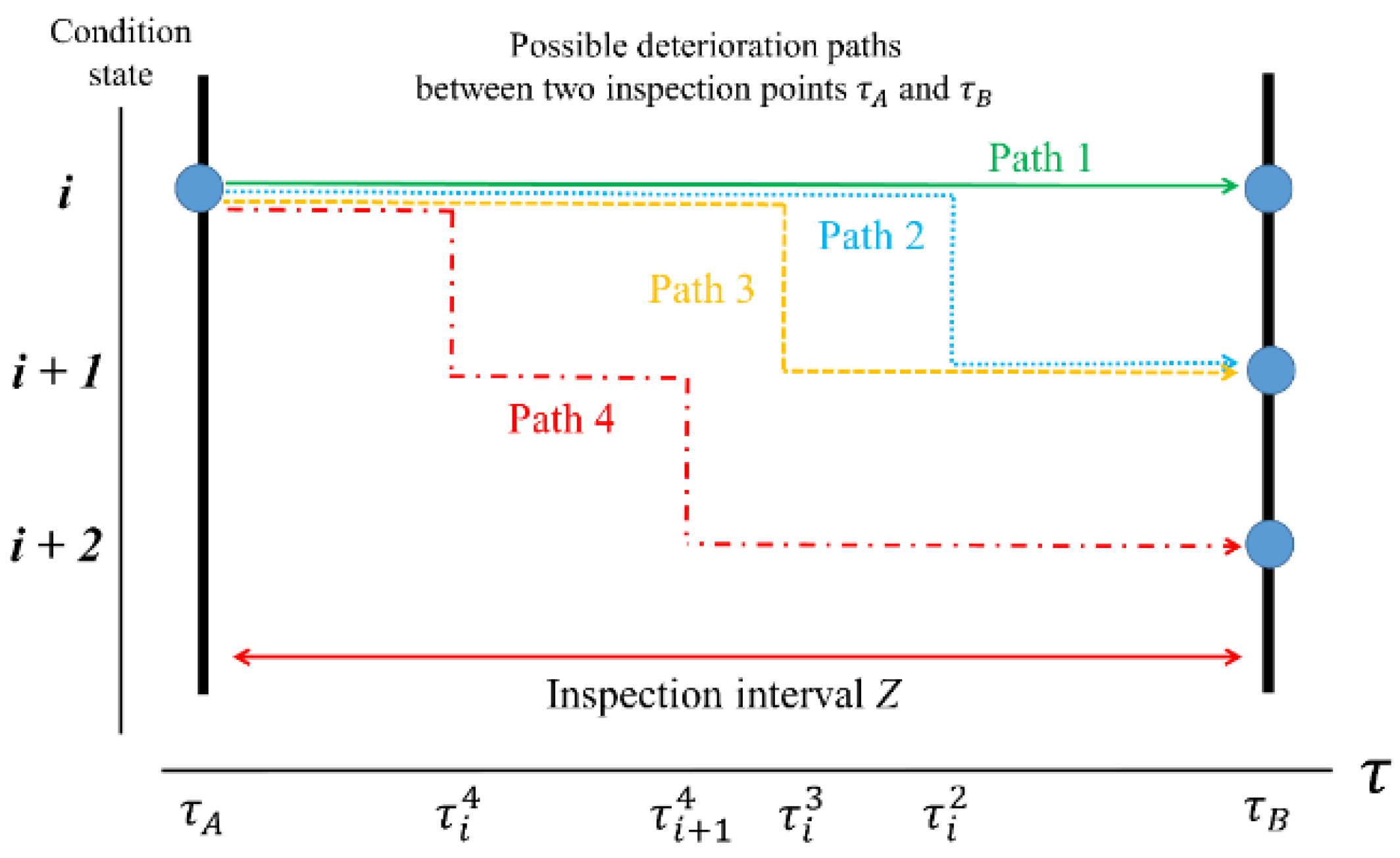
This section describes the BMMH model used for the deterioration process and risk analysis. The core part of the BMMH model lies in the structure of disassembling the Markov chain process into the multi-state hazard model. Here, the Markov chain expresses the continuous condition change of an object as a discrete condition state, and has possible deterioration paths within a specific time interval (See Figure 1 and Figure 2) [13,27].

With the condition state of a bridge defined as $i\left(i=1,\dots ,J\right)$, the condition state $i=1$ is defined as the best state that can be presented by an object, and $i=J$ as the absorbing state that represents the limit state of an object. Here, the time spent from $i=1$ to $i=J$ represents the life expectancy, and a set of probability elements to transfer from a certain state to another during the unit time interval $z\left(z={\tau }_B-{\tau }_A\right)$ represents the MTP matrix. The MTP matrix $\mathsf{\Pi }$ defined here and probability element ${\pi }_{ij}$ can be expressed as the following formula:

$$\mathrm{Prob}\left[h\left({\tau }_B\right)=j|h\left({\tau }_A\right)=i\right]={\pi }_{ij}$$

(1)

$$\mathsf{\Pi }=\left[\begin{array}{ccc}{\pi }_{11}& \cdots & {\pi }_{1J}\\ ⋮& \ddots & ⋮\\ 0& \cdots & {\pi }_{JJ}\end{array}\right]$$

(2)

There are several important preconditions for Equations (1) and (2). Given the assumption that the condition of an object changes over time, ${\pi }_{ij}\ge 0$ is validated, and $\sum _{j=1}^J{\pi }_{ij}=1$ is a natural condition according to the axiom of probability. As the deterioration model does not consider the improvement of condition state through maintenance, ${\pi }_{ji}=0\left(i>j\right)$ is validated, and the condition does not occur to the level below the absorbing state, so ${\pi }_{JJ}=1$ is validated.

Suppose that there is a bridge group or individual bridges with different deterioration characteristics among all bridges. If this bridge group is expressed as $k\left(k=1,\dots ,K\right)$, an individual bridge in each group can be expressed as $s_k\left(s=1,..,S;k=1,\dots ,K\right).$ In this case, the deterioration model representing all groups can be generalized as ${\lambda }_i$, the hazard function of the condition state of $i\left(i=1,\dots ,J-1\right)$, and the deterioration characteristics of each group can be explained with the adoption of ${\epsilon }^k$, the heterogeneous parameter of each group. The hazard mixing mechanism of the BMMH model can be expressed as the following formula:

$${\lambda }_i^{s_k}={\tilde{\lambda }}_i^{s_k}{\epsilon }^k \left(i=1,\dots ,J-1;s=1,\dots ,S;k=1,\dots ,K\right)$$

(3)

${\tilde{\lambda }}_i^{s_k}$ here is the average hazard function representing the collective samples, and the hazard function of each $k$ group is determined by reflecting ${\epsilon }^k$. Here, ${\epsilon }^k$ becomes non-negative ($0<{\epsilon }^k<\infty )$ because ${\epsilon }^k=1$ is the benchmarking function representing all sample groups. The heterogeneity function ${\epsilon }^k$ can be in the form of a function or stochastic variable that is assumed to be drawn from the gamma distribution ${\epsilon }^k~G\left(\alpha ,\gamma \right)$. It is expressed as the following formula:

$$f\left({\epsilon }^k:\alpha ,\gamma \right)=\frac{1}{{\gamma }^{\alpha }\mathsf{\Gamma }\left(\alpha \right)}{\left({\epsilon }^k\right)}^{\alpha -1}\exp \left(-\frac{{\epsilon }^k}{\gamma }\right)$$

(4)

The $\alpha$ and $\gamma$ here are the parameters of the gamma distribution, and $\mathsf{\Gamma }(·)$ is the CDF (Cumulative Distribution Function). The average and variance which are gamma distribution function $f\left({\epsilon }^k:\alpha ,\gamma \right)$ can be obtained from $\alpha \gamma$ and $\alpha {\gamma }^2$. Thus, the Probability Density Function (PDF) of the gamma distribution at $\alpha \gamma =1$ and $\alpha {\gamma }^2=1/\varphi$ is obtained by the following:

$$\overline{g}\left({\epsilon }^k:\varphi \right)=\frac{{\varphi }^{\varphi }}{\mathsf{\Gamma }\left(\varphi \right)}{\left({\epsilon }^k\right)}^{\varphi -1}\exp \left(-\varphi {\epsilon }^k\right)$$

(5)

The next formula represents the probability that the condition state does not change within the unit period, which can also be defined as the survival function $R_i\left(y_i^{s_k}\right)$ that has a longer life expectancy than that of $y_i^{s_k}$, as in the following formula:

$$R_i\left(y_i^{s_k}\right)=\exp \left(-{\tilde{\lambda }}_i^{s_k} {\overline{\epsilon }}^k y_i^{s_k}\right)$$

(6)

The bar $\left[¯\right]$ represents the value that is measurable. The following formula presents the multi-state exponential hazard function that is drawn from the generalization of Equation (6) by dividing it into probable condition change paths ${\pi }_{ii}$, ${\pi }_{i,i+1}$, ${\pi }_{ij}$, and ${\pi }_{iJ}$ during the unit time $z$, as follows:

$${\pi }_{ii}\left(z^{s_k}: {\overline{\epsilon }}^k\right)=\exp \left(-{\tilde{\lambda }}_i^{s_k} {\overline{\epsilon }}^k{z}^{s_k}\right)$$

(7)

$$\begin{gathered} {\pi }_{ij}\left(z^{s_k}: {\overline{\epsilon }}^k\right)={\displaystyle \sum }_{s=i}^j{\displaystyle \prod }_{m=i}^{j-1}\frac{{\tilde{\lambda }}_m^{s_k}}{{\tilde{\lambda }}_m^{s_k}-{\tilde{\lambda }}_s^{s_k}}\exp \left(-{\tilde{\lambda }}_i^{s_k} {\overline{\epsilon }}^k{z}^{s_k}\right)={\displaystyle \sum }_{s=i}^j{\psi }_{ij}^s\left({\tilde{\lambda }}_i^{s_k}\right) \exp \left(-{\tilde{\lambda }}_i^{s_k} {\overline{\epsilon }}^k{z}^{s_k}\right) \\ \mathrm{where}, {\psi }_{ij}^l\left({\tilde{\lambda }}^k\right)={{\displaystyle \prod }}_{m=i}^{j-1}\frac{{\tilde{\lambda }}_m^{s_k}}{{\tilde{\lambda }}_m^{s_k}-{\tilde{\lambda }}_s^{s_k}} \left(i=1,\dots ,J-1;j=i+1,\dots ,J;k=1,\dots ,K\right) \end{gathered}$$

(8)

Adding to it, the sum of the transition probability is ${\sum }_{j=1}^J{\pi }_{ij}=1$ and ${\pi }_{iJ}$, which reaches the final absorbing state. This can be formalized as Equation (9):

$${\pi }_{iJ}\left(z^{s_k}: {\overline{\epsilon }}^k\right)=1-{\displaystyle \sum }_{s=i}^{j-1}{\pi }_{ij}\left(z^{s_k}: {\overline{\epsilon }}^k\right)$$

(9)

Through Equations (7) to (9), the Markov chain process is decomposed using a multi-state exponential hazard function, and the mixing mechanism with the heterogeneous factor is normalized. In this format, however, explanatory variables that intervene in the deterioration process cannot be considered. The necessary structure here is adopting the explanatory variable ${\overline{x}}^{s_k}$ and the corresponding unknown parameter vector ${\beta }_i=\left({\beta }_{i,1},\dots ,{\beta }_{i,M}\right)$ to the parameter estimation. This structure can be expressed as the following formula:

$${\tilde{\lambda }}_i^{s_k}=f\left({\overline{x}}^{s_k}: {\beta }_i^{\prime }\right)=\exp \left({\overline{x}}^{s_k}: {\beta }_i^{\prime }\right)$$

(10)

That is, the MTP’s matrix element ${\pi }_{ij}$ is determined by the data set ${\xi }^{s_k}=\left({\overline{\delta }}^{s_k},{\overline{x}}^{s_k},{\overline{z}}^{s_k}\right)$. ${\overline{\delta }}^{s_k}$ here is a dummy variable, and whether the condition change occurs can be defined as 1 in case of $\overline{h}\left({\tau }_A^k\right)=i$ and $\overline{h}\left({\tau }_A^k\right)=j$, and 0 if not. For reference, ${}^{\prime }$ in Equation (10) means vector transpose. Ultimately, life expectancy for each condition state $L{E}_i^{s_k}$ can be obtained by the inverse function of the hazard function ${\tilde{\lambda }}_i^{s_k}\left(i=1,\dots ,J-1\right)$, and life expectancy $L{E}_{iJ}^{s_k}$ from the condition state $i$ to $J$ (or $j$), and is calculated by the sum of life expectancy of each condition state as follows:

$$L{E}_i^{s_k}={{\displaystyle \int }}_0^{\infty }{R}_i\left(y_i^{s_k}\right)d{y}_i^{s_k}={{\displaystyle \int }}_0^{\infty }\exp \left(-{\tilde{\lambda }}_i^{s_k}{y}_i^{s_k}\right)d{y}_i^{s_k}=\frac{1}{{\tilde{\lambda }}_i^{s_k}}$$

(11)

$$L{E}_{iJ}^{s_k}={\displaystyle \sum }_{i=1}^{J-1}L{E}_i^{s_k}$$

(12)

In sum, the application of the BMMH model boils down to the estimation of the unknown parameter ${\beta }_{i,M}$, ${\overline{\epsilon }}^k$, and the hyper parameter $\varphi$. If a traditional parametric method like MLE is used to estimate the parameter, ${\beta }_{i,M}$, $\varphi$, and ${\overline{\epsilon }}^k$ are estimated phase by phase (or hierarchically), which is inconvenient and is limited in that the distribution information of the parameter (and in turn, the hazard function and life expectancy) cannot be identified. The BMMH model resolves this problem by applying the MCMC, a non-parametric parameter estimation method.

The key to a successful MCMC lies in the designation of the initial value of parameters and sufficient sampling. The starting points (i.e., initial value) of the parameter sampling must be determined according to the analyst’s intuition. Starting from this initial value, the parameter value enters a convergence state in which a specific pattern is repeated in a specific area through sufficiently large sampling update processes. Samples before entering the convergence state are called burn-in samples, and these samples should be excluded from the derivation of parameter values. Whether or not the convergence state has kicked in should be determined directly by the analyst by referring to the form of a trace-plot that expresses the sample updating process of the MCMC, which often meets with ambiguity. An easy way to check whether the MCMC enters the convergence state is to designate the initial value of the parameter with a large deviation from the expected result value. This is because even if it takes a long time, it is easy to visually identify that the MCMC eventually moves to the convergence state with sufficiently large random walks. Meanwhile, there is a tendency that continuous sample rejects occur frequently or confusions in the non-convergence state are caused as the variance of parameters becomes excessively large. It can be solved by adjusting the stride of the random walk [24].

In fact, the MCMC method itself does not include a statistical test method for derived parameter values. Eventually, the key to this statistical test is to diagnose whether only the samples that reached the convergence state were used to derive the parameters. Many kinds of statistical methods have been proposed for this statistical test of the MCMC [28]. This study adopted Geweke’s z-score, which has been most commonly used for the MCMC test [37]. Due to the limits of space, please refer to the related literature for details on the theory and application method of the MCMC and Geweke’s test [24,28,37,38].

3. Empirical Study

3.1. Data Securing and Processing

It is important to secure enough samples to build a deterioration model based on the probability process. A data set was developed by matching diagnosis data obtained over 10 years for bridges in ROK with annual average traffic volume information. The data set for the application of the BMMH model consists of (1) before condition state $i\left({\tau }_A\right)$, (2) after condition state $j\left({\tau }_B\right)$, (3) time gap between the two condition states $z\left({\tau }_B-{\tau }_A\right)$, and (4) explanatory variable ${\overline{x}}^{s_k}$. The data with the increased condition state $i\left({\tau }_A\right)>i\left({\tau }_B\right)$ through maintenance works has been removed according to the preconditions proposed by Equations (1) and (2), and the final set of 30,040 pieces has been secured through the process of excluding the data set missing traffic information (${\overline{x}}^{s_k}$).

Table 2. Time-series data set by usage period.

Groups	Grouping Standard	Num. of Sample Set	AADT
Total (Benchmark)	All samples	30,040	32,164
Group A $=\left(e^{k\left(1\right)}\right)$	Less than 10 years	15,860	27,592
Group B $=\left(e^{k\left(2\right)}\right)$	10 to 20 years	11,686	38,693
Group C $=\left(e^{k\left(3\right)}\right)$	20 to 30 year	2048	31,252
Group D $=\left(e^{k\left(4\right)}\right)$	Over 30 years	446	27,855

summarizes basic information of the data collected according to the four periods of use.

3.2. Estimation of Deterioration Processes and Life Expectancies by Age Group

The BMMH model draws the life expectancy, deterioration curve, and MTP from the hazard function by condition state ${\theta }_i$. This hazard function is drawn from the unknown parameter ${\beta }_{i,m}$, ${\epsilon }^k,$ and the function of explanatory variable ${\overline{x}}_m^k$. This study conducted sampling 40,000 times; the initial 20,000 samples were discarded as burn-in samples, then 20,000 samples were used to derive the parameters.

Table 3. Parameters of the BMMH model by groups.

Condition State	Betas ${\mathit{\beta }}_{\mathit{i},\mathit{m}}$ (Geweke’s Z)		Explanatory Variables ${\overline{\mathit{x}}}_{\mathit{m}}^{\mathit{k}}$ (Normalized Value by (0,1])					Heterogeneity Factors ${\mathit{\epsilon }}^{\mathit{k}}$ (Geweke’s Z)
	${\mathit{\beta }}_{\mathit{i},0}$	${\mathit{\beta }}_{\mathit{i},1}$	Benchmark	${\overline{\mathit{x}}}_1^{\mathit{k}\left(1\right)}$	${\overline{\mathit{x}}}_1^{\mathit{k}\left(2\right)}$	${\overline{\mathit{x}}}_1^{\mathit{k}\left(3\right)}$	${\overline{\mathit{x}}}_1^{\mathit{k}\left(4\right)}$	Benchmark	${\mathit{\epsilon }}^{\mathit{k}\left(1\right)}$	${\mathit{\epsilon }}^{\mathit{k}\left(2\right)}$	${\mathit{\epsilon }}^{\mathit{k}\left(3\right)}$	${\mathit{\epsilon }}^{\mathit{k}\left(4\right)}$
A to B	−1.34	0.16	0.099	0.085	0.119	0.096	0.086	1.000	0.181	0.335	0.285	2.943
	(0.09)	(0.01)
B to C	−3.73	0.87							(−0.11)	(−0.09)	(−0.05)	(0.003)
	(0.09)	(−0.06)

and

Table 4. Hazard functions and life expectancies by groups.

Condition State	Hazard Functions ${\mathit{\lambda }}_{\mathit{i}}^{\mathit{k}}$					Life Expectancy (Year) $\mathit{L}{\mathit{E}}_{\mathit{i}}^{\mathit{k}}$
	Benchmark	Group 1	Group 2	Group 3	Group 4	Benchmark	Group 1	Group 2	Group 3	Group 4
A to B	0.267	0.048	0.090	0.076	0.785	3.74	20.68	11.13	13.14	1.27
B to C	0.026	0.005	0.009	0.007	0.076	38.25	213.43	112.07	134.53	13.14
Total life expectancy (year)						41.99	234.12	123.20	147.68	14.41

and Figure 3 and Figure 4 put together the estimated values of parameters, Geweke test values, hazard functions, and life expectancy.

Table 3 shows that the values of Geweke-Z of ${\beta }_{i,m}$ and ${\epsilon }^k$ drawn from the MCMC are all close to 0, the optimal value. This means that only the samples that reached the convergence state were well-utilized to derive the parameter, and this can be easily confirmed through Figure 3. Furthermore, the value of ${\beta }_{i,1}$ corresponding to the traffic volume applied as an explanatory variable is all drawn as (+) value, confirming that it is inversely related to life expectancy. Meanwhile, the value of ${\epsilon }^k$ indicating the heterogeneous deteriorating speed of each group indicates that groups A, B, and C have long life expectancies compared to the benchmark, which is less than 1, but aging bridge group D has a very high value of 2.93.

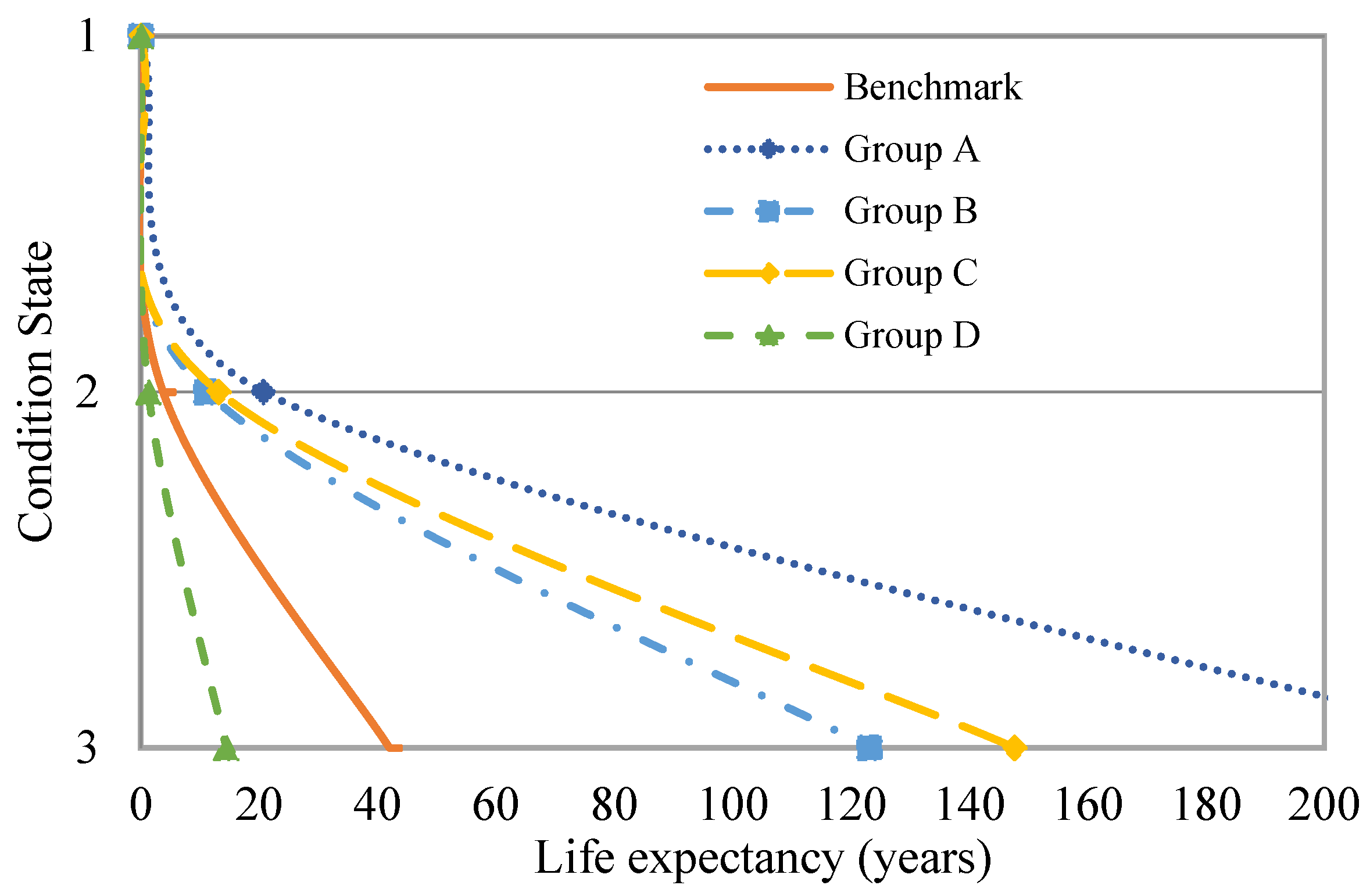
The comparison of characteristics of life expectancy according to group suggested in Table 4 and Figure 4 shows the tendency that the group of bridges with an age of less than 10 years has the longest life expectancy, and the life expectancy shortens as the period of use is prolonged. Particularly, the life expectancy of old bridges with more than 30 years of use was 14.4 years, which is one-third the average life expectancy among the network of 41.99 years. This means that old bridges reach grade C after an average of 14.4 years, even if their current condition is grade A. The fact that the life expectancy of group B is longer than that of group C is not in line with the general trend. It is considered as a bias of the sample used for analysis, since the deviation was relatively short compared to the entire life expectancy. It is necessary to conduct a follow-up study on the reasons for such deviation (e.g., construction standards, technology, materials, management policies, etc.).

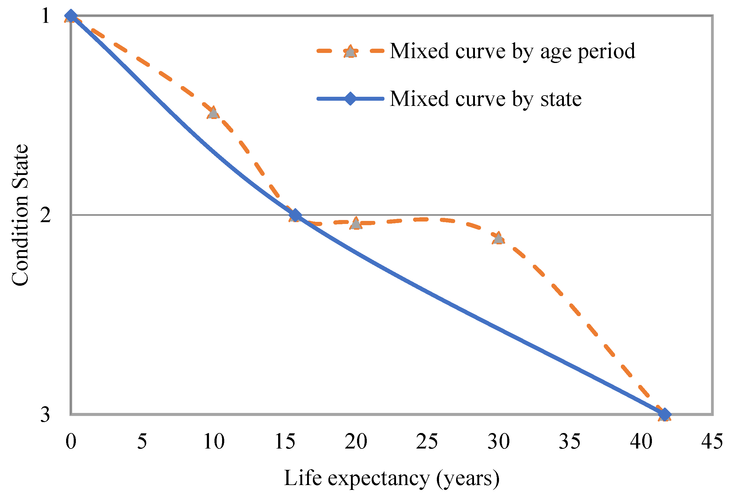
It should be noted that there might be an error in interpreting the life expectancy of each group, due to the characteristics of developing the deterioration model by dividing it by the period of use. For example, the life expectancy of group A is more than 200 years, resulting in somewhat abnormal values. This means that the physical conditions or durability of a new bridge are maintained regardless of the lapse of time. The expiration date of the deterioration model of group A is 10 years, and the deterioration characteristics of group B→C→D appear in order.

Table 5. Sequential deterioration process.

Referred Deterioration Functions	Annual Condition Degrade Function	Duration (Year)	Cumulated Life Expectancy (Year)
Group1/State 1	0.0483	10.00	10.00
Group2/State 1	0.0898	5.75	15.75
Group2/State 2	0.0089	4.25	20.00
Group3/State 2	0.0074	10.00	30.00
Group4/State 2	0.0761	11.66	41.66

and Figure 5 show the linked deterioration process considering the change in deterioration characteristics over time.

Figure 5 compares the deterioration curves created by classifying them by condition state and period of use. With this, it is possible to confirm the characteristics of the change in the deterioration rate within the state, which is not known by the Markov chain process that is expressed based on the state. One notable feature here is that it maintains a slow deterioration rate for a relatively long period of time after reaching State B, and then rapid deterioration begins from 30 years of use. This reflects the characteristics of ROK’s management, in which small-scale preventive maintenance is implemented when State B is reached, while almost no action is taken for the condition State A. This means that when a certain state is reached, there is a period (or condition) in which preventive maintenance cannot prevent the state from deteriorating to State C.

3.3. Analysis of the Risk of Deficiency by Age Group

This study defines State C as defective and the sum of the transition probability of State A→C and State B→C as a risk (i.e., POF). Here the level of risk is compared by deriving the standard MTP ($\mathsf{\Pi }$) for each group derived using the hazard function of each group (Refer to Equations (7)–(9)). The results are shown in

Table 6. Comparison of Markov transition probability metrics by usage groups ($z$ = 1 year).

State	Benchmark			Group A			Group B			Group C			Group D
	A	B	C	A	B	C	A	B	C	A	B	C	A	B	C
A	0.766	0.231	0.003	0.953	0.047	0.0001	0.914	0.086	0.0004	0.927	0.073	0.0003	0.456	0.536	0.008
B	-	0.974	0.026	-	0.995	0.0047	-	0.991	0.0089	-	0.993	0.0074	-	0.974	0.026
C	-	-	1.000	-	-	1.0000	-	-	1.0000	-	-	1.0000	-	-	1.000
POF	2.90%			0.48%			0.93%			0.77%			3.38%

.

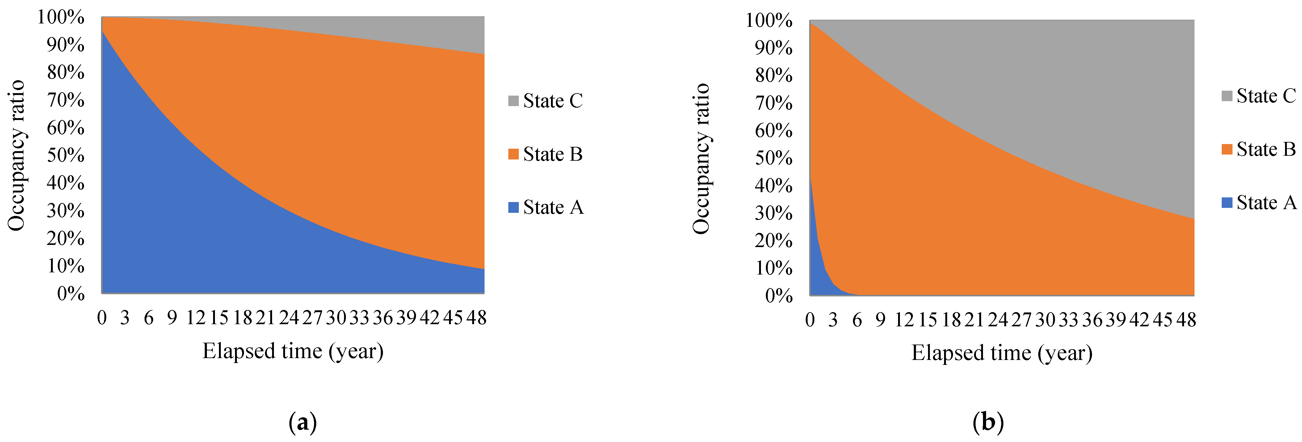
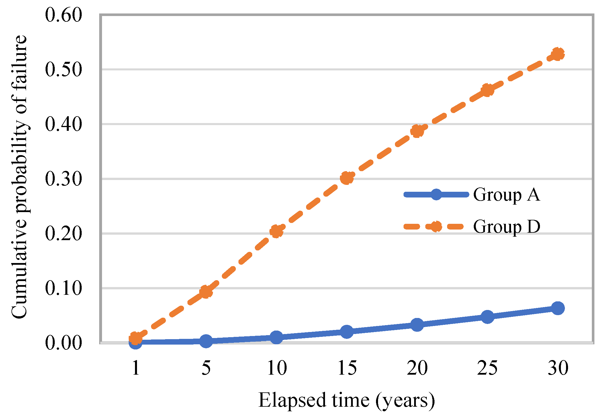
It is shown in Table 6 that the summation of probability of failure of Group D is 3.38%, which is 7.05 times higher than that of Group A within 10 years of construction. This means that more frequent diagnosis and rehabilitation are required, and also that the unit cost of bridge management is higher. Implementing the update of state by applying the Chapman–Kolmogorov equation (${\mathsf{\Pi }}^{\left(m+n\right)}={\mathsf{\Pi }}^{\left(m\right)}{\mathsf{\Pi }}^{\left(n\right)}$) on the assumption that the characteristics of such condition transitions are maintained can estimate the changing process of ratio in the condition state of bridge networks. The comparison of the condition updating of Group A and Group D with the most pronounced deviation is shown in Figure 6 and Figure 7 and

Table 7. Comparison of POFs at time points between Group A and D.

Elapsed Time (Year)	POF of Group A	POF of Group D	Times (Group D/A)
1	0.0001	0.0080	71.5
5	0.0026	0.0930	35.8
10	0.0095	0.2036	21.3
15	0.0198	0.3011	15.2
20	0.0325	0.3868	11.9
25	0.0471	0.4619	9.8
30	0.0631	0.5279	8.4

.

A significant difference in characteristics of network condition updating between the two groups is shown in Table 7 and Figure 6 and Figure 7. The difference in POF is 21.3 times for the warranty period of 10 years, 11.9 times for the useful life of 20 years under the National Accounting Law, and 8.4 times for the standard period of 30 years for aging bridges. It is easy to predict a scenario in which the ratio of old bridges continuously increases over time, and accordingly, the demand and cost of maintenance increase exponentially.

3.4. Maintenance Demand to Achieve the Target Level of Risk Management-Example

The long-term maintenance strategy and maintenance demand (quantity) of the bridge network in ROK have been estimated using the previously derived MTP ($\mathsf{\Pi }$). The maintenance strategy here will be defined as “What minimum percentage of State C quantities must be continuously maintained to achieve the target level of 95% in risk management?” This is a simple but robust strategy that guarantees the organization’s goal while preventing a peak of budget demand.

When multiplying ${\mathsf{\Pi }}^{\left(m\right)}$, the current state ratio of the bridge network under management, by ${\mathsf{\Pi }}^{\left(n\right)}$, $n$^th year’s transition probability reflecting the maintenance strategy ${\pi }_{Ji}$, and with continuous updating, the convergence state is reached, in which all elements of ${\mathsf{\Pi }}^{\left(m+n\right)}$ do not change anymore. Simply put, it is the process of finding the optimal solution of ${\pi }_{Ji}$, where the convergence value reaches 95%. Meanwhile, different ${\pi }_{Ji}$ may be applicable according to the level or types of repair methods, but it is assumed that the simplest strategy is applied, which is a complete recovery of conditions, or ${\pi }_{31}\left(J=3,i=1\right)$. It is also assumed that the characteristics of condition transition and the number of bridges do not change during the analysis period. For reference, as this analysis targets the entire bridge network, the MTP of the benchmark case is applied.

To apply this methodology, it is necessary to define ${\mathsf{\Pi }}^{\left(m\right)}$, the composition ratio of initial condition state. As of 2020, the number of bridges managed by the central government of ROK is 18,598, and the ratios of States A, B, C, and below correspond to 27.3%, 67.3%, and 5.4%, respectively. That is, the current risk management level is 94.6% (see

Table 8. Bridge condition in ROK for definition of the ${\mathsf{\Pi }}^{\left(m\right)}$ (managed by central government).

Total Number	A Grade	B Grade	C–E Grades	Note
18,598	5078	12,517	1003	Including expressway, national highways, and privately funded roads
(100.0%)	(27.3%)	(67.3%)	(5.4%)

) [31].

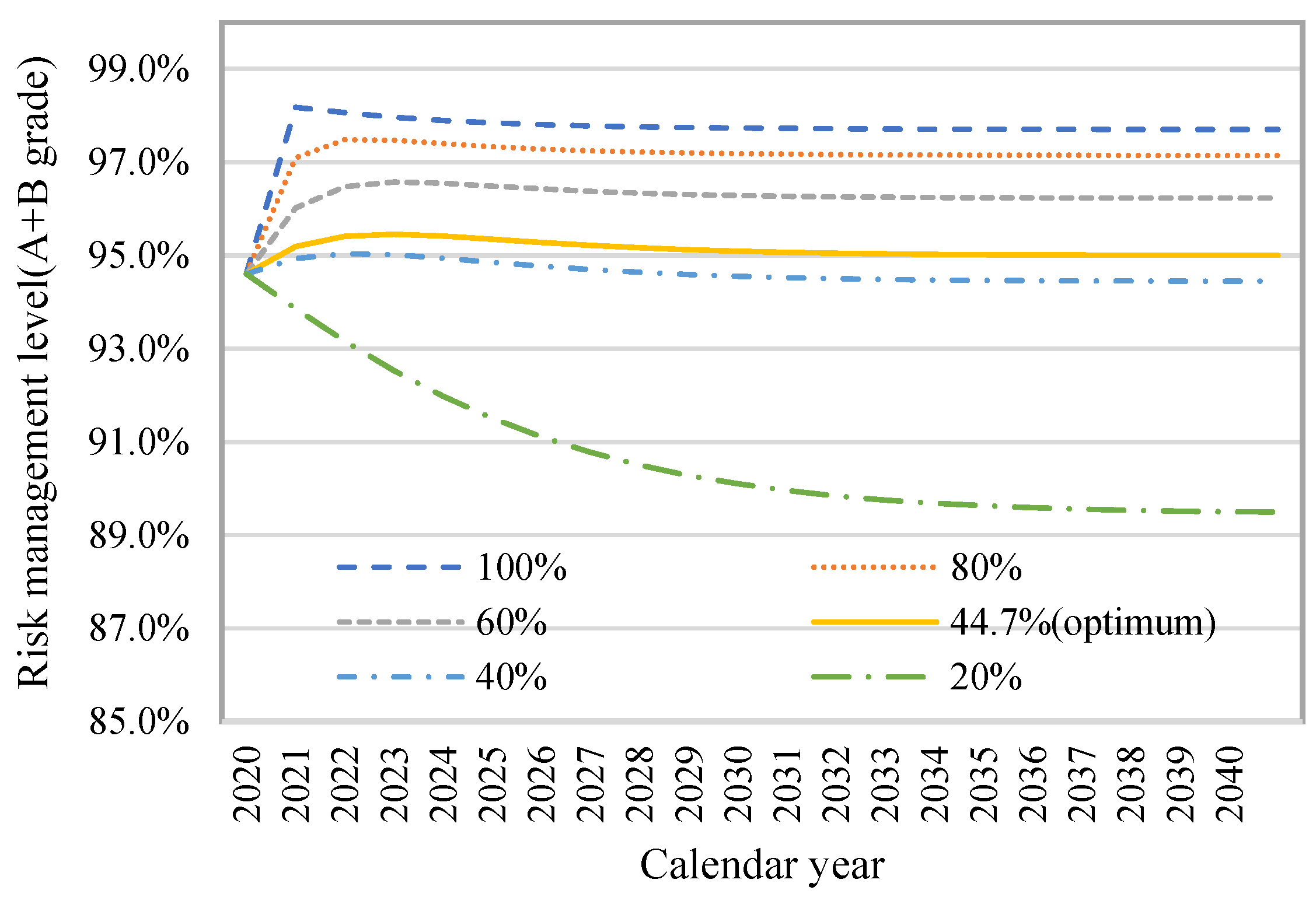
The analysis on the sensitivity of ${\pi }_{31}$ with a 10% gap showed that the possible level of risk management to be secured was from 97.7% (${\pi }_{31}$=1, ${\pi }_{33}=0$) to 81.0% (${\pi }_{31}$=0.1, ${\pi }_{33}=0.9$). Within the range, the optimal solution of ${\pi }_{31}$ that comes down to 95.0% was 44.7%.

Table 9. Condition update of bridge network in ROK at the optimal ${\pi }_{31}=0.447$.

Year	A Grade	B Grade	C~E Grades	Risk Management Level (=A + B Grade)	Maintenance Demands
2020	0.273	0.673	0.054	94.60%	1004
2021	0.233	0.719	0.048	95.19%	895
2022	0.200	0.754	0.046	95.41%	853
2023	0.174	0.781	0.045	95.45%	846
2024	0.153	0.801	0.046	95.41%	853
2025	0.138	0.816	0.047	95.35%	865
2026	0.126	0.826	0.047	95.28%	878
2027	0.118	0.834	0.048	95.22%	890
2028	0.112	0.840	0.048	95.16%	899
2029	0.107	0.844	0.049	95.12%	907
2030	0.104	0.847	0.049	95.09%	913
2031	0.101	0.849	0.049	95.07%	918
2032	0.100	0.851	0.050	95.05%	921
2033	0.098	0.852	0.050	95.03%	924
2034	0.098	0.853	0.050	95.02%	925
2035	0.097	0.853	0.050	95.02%	927
2036	0.096	0.854	0.050	95.01%	928
2037	0.096	0.854	0.050	95.01%	928
2038	0.096	0.854	0.050	95.00%	929
2039	0.096	0.854	0.050	95.00%	929
2040	0.096	0.854	0.050	95.00% (Converged)	930

and Figure 8 and Figure 9 show the information of the change in network conditions at ${\pi }_{31}=0.447$.

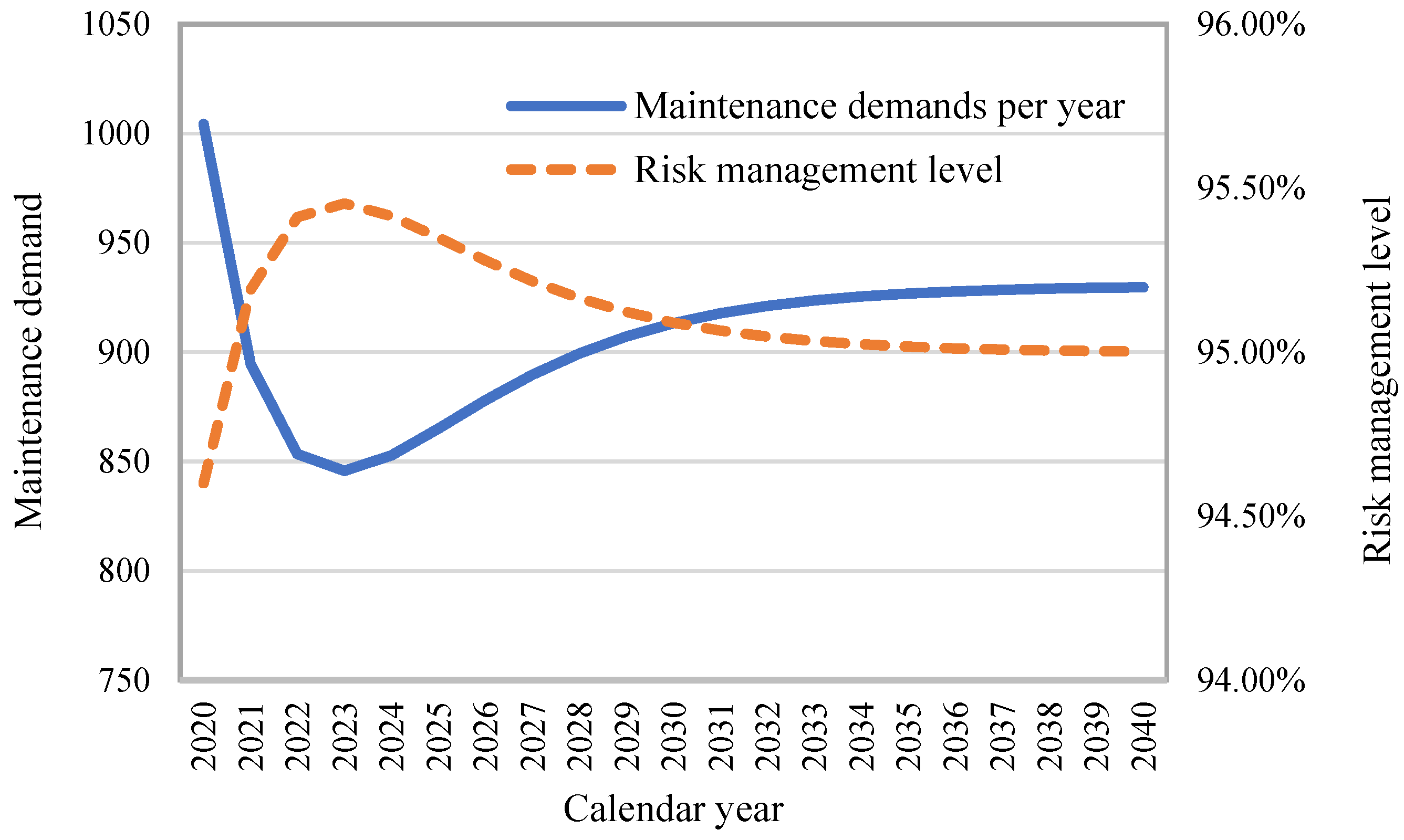
Summarizing Table 9 and Figure 8 and Figure 9, 44.7% of bridges in State C must go through maintenance every year for continuous achievement of the goal. In 2040, 20 years later, the risk management level and annual demand of repair converge into 95% and 930 cases (i.e., 5% of the total), respectively.

4. Discussion

A major achievement of this study is to confirm that the deterioration rate of aging bridges that have been used for more than 30 years is heterogeneously fast. The main results can be summarized as follows:

• The life expectancy of old bridges used for more than 30 years is 14.4 years, which is 1/3 of the network average of 41.9 years.
• The probability of deficiencies of the old bridges is seven times higher than that of new bridges of 10 years old or less.
• Preventive maintenance can help prolong the life expectancy of a bridge; however, it cannot completely prevent the deterioration of the condition grade.
• In order to keep the bridge management risk level of ROK above 95% of A + B Grade, 44.7% of Grade C bridges must be continuously maintained every year.

Future studies will focus on the increasing trends of annual budget demands, the timing of peak occurrence, and strategies for distributing this peak through life cycle cost analysis that reflects the trend of the increase in aging bridges. Above all, the development of deterioration models for each bridge member, effects of various explanatory variables (environmental condition, structural types, scale, material characteristics, etc.) on the deterioration process, and approaches to the consequence of failure, which were not covered in this study, are also essential topics for precise and reliable asset management.

References

- ISO (International Organization for Standardization). ISO 55000:2014 Asset Management-Overview, Principles and Terminology; International Organization for Standardization: Geneva, Switzerland, 2014; p. 14. [Google Scholar]
- ISO (International Organization for Standardization). ISO 55001:2014 Asset Management-Management Systems-Requirements; International Organization for Standardization: Geneva, Switzerland, 2014; pp. 4–5. [Google Scholar]
- IPWEA (Institute of Public Works Engineering Australasia). International Infrastructure Management Manual (International Edition 2015, 5th ed.; Institute of Public Works Engineering Australasia: North Sydney, Australasia, 2015; pp. 3|35–3|58. [Google Scholar]
- ASTM (American Society for Testing and Material). Standard Classification for Bridge Elements–Uniformat II (E2103/E2103M-19); ASTM International: West Conshohocken, PA, USA, 2019; pp. 1–21. [Google Scholar]
- ASCE (American Society of Civil Engineers). 2021 Infrastructure Report Card for America’s Infrastructure; American Society of Civil Engineers: Washington, DC, USA, 2020; pp. 18–25. [Google Scholar]
- Srikanth, I.; Arockiasamy, M. Deterioration models for prediction of remaining useful life of timber and concrete bridges: A review. J. Traffic Transp. Eng. 2020, 7, 152–173. [Google Scholar] [CrossRef]
- Wikipeida. Available online: https://en.wikipedia.org/wiki/Seongsu_Bridge (accessed on 15 May 2021).
- Wikipeida. Available online: https://en.wikipedia.org/wiki/List_of_bridge_failures (accessed on 15 May 2021).
- Ford, K.M.; Arman, M.; Labi, S.; Sinha, K.C.; Ashirole, A.; Thompson, P.; Li, Z. Methodology for Estimating Life Expectancies of Assets, Draft Final Report of NCHRP Project 08-17; Purdue University: West Lafayette, IN, USA, 2011; pp. 54–56. [Google Scholar]
- Estes, A.C.; Frangopol, D.M. Repair optimization of highway bridges using system reliability approach. J. Struct. Eng. 1999, 125, 766–775. [Google Scholar] [CrossRef] [Green Version]
- Sinha, K.C.; Labi, S.A.; McCullouch, B.G.; Bhargava, A.; Bai, Q. Updating and Enhancing the Indiana Bridge Management System (IBMS), Volume 1 (Technical Manual); Publication FHWA/IN/JTRP-2008/30; Indiana Department of Transportation and Purdue University: West Lafayette, IN, USA, 2009; pp. 97–107. [Google Scholar]
- Cope, A.R. Multiple-Criteria Life-Cycle Evaluation of Alternative Bridge Deck Reinforcement Materials Using Rank Matrix Analysis. Ph.D. Thesis, Purdue University, West Lafayette, IN, USA, 2009. [Google Scholar]
- Tsuda, Y.; Kaito, K.; Aoki, K.; Kobayashi, K. Estimating Markovian transition probabilities for bridge deterioration forecasting. J. Struct. Eng. Earthq. Eng. 2006, 23, 241s–256s. [Google Scholar] [CrossRef] [Green Version]
- Hallberg, D. Development and Adaptation of a Life Cycle Management System for Developed Work. Ph.D. Thesis, KTH Royal Institute of Technology, Stockholm, Sweden, 2005. [Google Scholar]
- Saeed, T.U.; Moomen, M.; Ahmed, A.; Murillo-Hoyos, J.; Volovski, M.; Labi, S. Performance evaluation and life prediction of highway concrete bridge superstructure across design types. J. Perform. Constr. Facil. 2017, 31, 1–14. [Google Scholar] [CrossRef]
- Lavrenz, S.M.; Saeed, T.U.; Murillo-Hoyos, J.; Volovski, M.; Labi, S. Can interdependency considerations enhance forecasts of bridge infrastructure condition? evidence using a multivariate regression approach. Struct. Infrastruct. Eng. 2020, 16, 1177–1185. [Google Scholar] [CrossRef]
- Saeed, T.U.; Qiao, Y.; Chen, S.; Alqadhi, S.; Zhang, Z.; Labi, S.; Sinha, K.C. Effects of Bridge Surface and Pavement Maintenance Activities on Asset Rating; Publication FHWA/IN/JTRP-2017/19; Indiana Department of Transportation and Purdue University: West Lafayette, IN, USA, 2017; pp. 1–56. [Google Scholar] [CrossRef]
- Saeed, T.U.; Qiao, Y.; Chen, S.; Gkritza, K.; Labi, S. Methodology for probabilistic modeling of highway bridge infrastructure condition: Accounting for improvement effectiveness and incorporating random effects. J. Infrastruct. Syst. 2017, 23, 1–11. [Google Scholar] [CrossRef]
- Wan, C.; Zhou, Z.; Li, S.; Ding, Y.; Xu, Z.; Yang, Z.; Xia, Y.; Yin, F. Development of a bridge management system on the building information modeling technology. Sustainability 2019, 11, 4583. [Google Scholar] [CrossRef] [Green Version]
- Safi, M.; Sundquist, H.; Karoumi, R. Cost-efficient procurement of bridge infrastructures by incorporating life-cycle cost analysis with bridge management systems. J. Bridge Eng. 2014, 20, 1–12. [Google Scholar] [CrossRef]
- Teresa, M.A.; Juni, E. Element Unit and Failure Costs and Functional Improvement Costs for Use in the Mn/DOT Pontis Bridge Management System; Minnesota Department of Transportation: St. Paul, MN, USA, 2003; pp. 1–51.
- Han, D. Empirical evaluation of utility of anti-frost layer in pavement structure considering regional climate characteristics. Intl. J. Pavement Eng. 2021, 1–8. [Google Scholar] [CrossRef]
- Kaito, K.; Kobayashi, K. Bayesian estimation of markov deterioration hazard model. J. Jpn. Soc. Civ. Eng. Part A 2007, 63, 336–355. (In Japanese) [Google Scholar] [CrossRef] [Green Version]
- Han, D.; Kaito, K.; Kobayashi, K. Application of bayesian estimation method with markov hazard model to improve deterioration forecasts for infrastructure asset management. KSCE J. Civ. Eng. 2014, 18, 2107–2119. [Google Scholar] [CrossRef]
- Obama, K.; Okada, K.; Kaito, K.; Kobayashi, K. Disaggregated hazard rates evaluation and bench-marking. J. Jpn. Soc. Civ. Eng. 2008, 64, 857–874. (In Japanese) [Google Scholar] [CrossRef] [Green Version]
- Kaito, K.; Kobayashi, K.; Aoki, K.; Matsuoka, K. Hierarchical bayesian estimation of mixed hazard models. J. Jpn. Soc. Civ. Eng. 2012, 68, 255–271. (In Japanese) [Google Scholar] [CrossRef] [Green Version]
- Han, D.; Lee, S. Stochastic forecasting of life expectancies considering multi-maintenance criteria and localized uncertainty in the pavement-deterioration process. J. Test. Eval. 2016, 44, 128–140. [Google Scholar] [CrossRef]
- Han, D.; Kaito, K.; Kobayashi, K.; Aoki, K. Performance evaluation of advanced pavement materials by bayesian markov mixture hazard model. KSCE J. Civ. Eng. 2017, 20, 729–737. [Google Scholar] [CrossRef]
- Train, K.E. Discrete Choice Methods with Simulation, 2nd ed.; Cambridge University Press: New York, NY, USA, 2009; pp. 199–202. [Google Scholar]
- MOLIT (Ministry of Land, Infrastructure and Transport). Basic Act on Sustainable Infrastructure Management.; National Act-17237; Ministry of Land, Infrastructure and Transport: Sejong-Si, Korea, 2020; p. 1. (In Korean)
- MOLIT (Ministry of Land, Infrastructure and Transport). Development of 1st Road Infrastructure Management Plan (2020~2025); Ministry of Land, Infrastructure and Transport: Sejong-Si, Korea, 2020; pp. 33–144. (In Korean)
- MOLIT (Ministry of Land, Infrastructure and Transport). Yearbook of Road Bridge and Tunnel Statistics in 2020; 11-1613000-000108-10; Ministry of Land, Infrastructure and Transport: Sejong-Si, Korea, 2020; p. 4. (In Korean)
- MOLIT (Ministry of Land, Infrastructure and Transport). Detailed Guidelines for Safety Inspection and Precise Safety Diagnosis-Bridge; RD-12-E6-024; Ministry of Land, Infrastructure and Transport: Sejong-Si, Korea, 2021; pp. 235–236. (In Korean)
- MOEF (Ministry of Economy and Finance). Guidelines for Accounting for Depreciation of Intangible and Intangible Assets; Ministry of Economy and Finance: Sejong-Si, Korea, 2011; p. 6. (In Korean)
- MOLIT (Ministry of Land, Infrastructure and Transport). Evaluation Standard for Performance Improvement Project of Road Facilities; Government Notice–2021/213; Ministry of Land, Infrastructure and Transport: Sejong-Si, Korea, 2021; pp. 7–16. (In Korean)
- MOLIT (Ministry of Land, Infrastructure and Transport). Management Standards for Road Facilities; Government Notice-2021/214; Ministry of Land, Infrastructure and Transport: Sejong-Si, Korea, 2021; p. 6. (In Korean)
- Geweke, J. Evaluating the accuracy of sampling-based approaches to the calculation of posterior moments. In Bayesian Statistics, 4th ed.; Bernardo, J.M., Berger, J.M., Dawid, A.P., Smith, A.F.M., Eds.; Oxford University Press: Oxford, UK, 1992; pp. 169–193. [Google Scholar]
- Koop, G.; Poirier, D.J.; Tobias, J.L. Bayesian Econometric Methods; Cambridge University Press: New York, NY, USA, 2007; pp. 128–157. [Google Scholar]
Figure 1.
Discrete condition changes in Markov chain [27].
Figure 2.
Possible deterioration paths between two inspection points [27].
Figure 3.
Trace-plots of the MCMC process: (a) , (b) .
Figure 4.
Comparison of deterioration process by age groups.
Figure 5.
Sequentially mixed deterioration curves by condition state and usage period.
Figure 6.
Network bridge condition update: (a) Group A, (b) Group D.
Figure 7.
Comparison of cumulative POF between Group A and D.
Figure 8.
Sensitivity of risk management levels by maintenance strategy.
Figure 9.
Risk management level and maintenance demand at the optimal .