
Comparing Methods for Segmenting Supra-Glacial Lakes and Surface Features in the Mount Everest Region of the Himalayas Using Chinese GaoFen-3 SAR Images

1
Key Laboratory of Digital Earth Science, Aerospace Information Research Institute, Chinese Academy of Sciences, No. 9 Dengzhuang South Road, Beijing 100094, China
2
University of Chinese Academy of Sciences, Beijing 100049, China
3
Hainan Key Laboratory of Earth Observation, Aerospace Information Research Institute, Chinese Academy of Sciences, Sanya 572029, China
Remote Sens. 2021, 13(13), 2429; https://doi.org/10.3390/rs13132429
Submission received: 22 April 2021
/
Revised: 17 June 2021
/
Accepted: 18 June 2021
/
Published: 22 June 2021
(This article belongs to the Special Issue Applications of Remote Sensing in Glaciology)
Abstract
:Glaciers and numerous glacial lakes that are produced by glacier melting are key indicators of climate change. Often overlooked, supra-glacial lakes develop in the melting area in the low-lying part of a glacier and appear to be highly variable in their size, shape, and location. The lifespan of these lakes is thought to be quite transient, since the lakes may be completely filled by water and burst out within several weeks. Changes in supra-glacial lake outlines and other surface features such as supra-glacial rivers and crevasses on the glaciers are useful indicators for the direct monitoring of glacier changes. Synthetic aperture radar (SAR) is not affected by weather and climate, and is an effective tool for study of glaciated areas. The development of the Chinese GaoFen-3 (GF-3) SAR, which has high spatial and temporal resolution and high-precision observation performance, has made it possible to obtain dynamic information about glaciers in more detail. In this paper, the classical Canny operator, the variational B-spline level-set method, and U-Net-based deep-learning model were applied and compared to extract glacial lake outlines and other surface features using different modes and Chinese GF-3 SAR imagery in the Mount Everest Region of the Himalayas. Particularly, the U-Net-based deep-learning method, which was independent of auxiliary data and had a high degree of automation, was used for the first time in this context. The experimental results showed that the U-Net-based deep-learning model worked best in the segmentation of supra-glacial lakes in terms of accuracy (Precision = 98.45% and Recall = 95.82%) and segmentation efficiency, and was good at detecting small, elongated, and ice-covered supra-glacial lakes. We also found that it was useful for accurately identifying the location of supra-glacial streams and ice crevasses on glaciers, and quantifying their width. Finally, based on the time series of the mapping results, the spatial characteristics and temporal evolution of these features over the glaciers were comprehensively analyzed. Overall, this study presents a novel approach to improve the detection accuracy of glacier elements that could be leveraged for dynamic monitoring in future research.
1. Introduction
Glaciers are very sensitive to atmospheric climate change. The Tibet Plateau (TP) has the largest reserves of glaciers outside of the Antarctic and Arctic [1,2]. In recent decades, most TP glaciers have experienced accelerated thinning and melting. This has been accompanied by the formation and evolution of a large number of glacial lakes, and may also induce secondary glacial lake outburst flood (GLOF)-related disasters [3]. The high proportion of glacial lakes combined with the dynamic nature of the glaciated environment has made the TP a focus of lacustrine research [4,5,6]. Research regarding the identification and extraction of glacial lake outlines is an important first step for the assessment of regional water resources, prediction of GLOF events, and the study of climate-change impacts.
Previously, lake extents were mainly derived using manual delineation [1,7,8]. However, this is a time-consuming method. The accuracy and degree of details in the mapped glacial lake outlines are unstable and depend on subjective experience and operational procedures. Remote sensing is widely used to investigate glaciers and glacial lakes due to the wide areal coverage and long-term observation records of such data [9,10,11]. Investigations of spatio-temporal lake dynamics in the TP have made use of optical remote-sensing images such as those from Landsat series satellites [12,13], ASTER [14], and multi-spectral MODIS [15]. However, for the coverage of mountainous regions with harsh climate conditions, these images are generally limited by their low quality of observations. SAR has proven to be a useful and promising tool in glaciology due to its all-weather, day-and-night capabilities [16,17]. It is also an active emitting electromagnetic system with a flexible design for different modes of data in terms of frequency, polarization, and incidence angle. In addition, SAR is sensitive to surface roughness and dielectric properties, providing a feasible approach for distinguishing glacial lakes and different glacial facies [16].
When using remote-sensing images, different image detection and classification methods for the delineation of glacial lakes are favored (Table 1). Edge detection is a very important method in the field of image analysis and recognition. The purpose of edge detection is to find the collection of pixels whose brightness changes dramatically in the image [18]. Studies utilizing edge detection have focused on the extraction of glacier outlines by the Canny edge operator [17], and identification of linear features such as outlines and textural features of glacial lakes using a phase-congruency-based detector [19]. For automatic methods to extract glacial lakes, image segmentation has made a very important contribution. Thresholding is a simple and commonly used technique for image segmentation. An automated scheme of lake mapping based on hierarchical image segmentation and terrain analysis was proposed in [13]. Based on this method, a new method that utilized log-transformed spectral data and a normalized difference water index (NDWI), NDWIblue, for mapping glacial lakes partially obscured by mountain shadows was introduced [20]. Using automatically determined, lake-specific NDWI thresholds, the adaptive mapping algorithms implemented through image segmentation, at both global and local levels, proved to be robust and reliable for delineating lake boundaries under various complex water conditions at continental scales [21]. Combining a water index with digital image-processing technology, an automatic lake-extraction method was proposed to identify water pixels, especially mixed water pixels in shallow or narrow water bodies [22]. In order to detect supra-glacial lake area in Northeast Greenland, the potential of Sentinel-2 images was explored in a fully automated way, and the complete algorithm was presented, allowing for continuous monitoring [23]. Apart from the threshold segmentation, other groups of image-segmentation methods, such as active contour models, superpixel segmentation, and watershed segmentation, were gradually developed and applied. An image can be partitioned by computing the patch statistics in the image and then segmenting the image using an active contour model [12,24,25,26]. These level-set-based segmentation algorithms were further improved for the efficient extraction of small, overlooked glacial lakes and the removal of mountain shadows. Superpixel segmentation can effectively preserve the statistical characteristics of the image and segment image into many small homogeneous regions with similar sizes or with different scales [27,28]. To deal with the over-segmentation problems, solutions were based on a morphological approach that combined the watershed segmentation with average contrast maximisation [29,30]. Meanwhile, some object-oriented classification methods have also been developed to map glacial lakes [31,32]. These methods use characteristics of glacial lakes and their surroundings to differentiate between lake water and background, exploiting the full range of lake morphologies, spectral features, and contextual information. The smoothness of the border, as well as the homogeneity and compactness of the objects, are taken into account in the object-segmentation process [33].
In general, the use of satellite images for the monitoring of glacial lakes has been mostly concerned with conventional manual digitization, edge detection, image segmentation methods, and object-oriented classification, rarely adopting some advanced deep-learning methods. Compared with other methods, deep-learning algorithms have a high ability in terms of feature extraction and autonomous learning; they possess a large number of hidden layers and can support a higher level of data abstraction and prediction. These advantages mean that these algorithms have broad prospects in cryosphere applications. An attempt has been made recently to map glacial lakes using deep-learning models. Wu et al., 2020 presented an improved U-Net-based, deep-learning, semantic-segmentation network model for extracting the unconnected small glacial lake outlines using a combination of Sentinel-1 ground-range-detected (GRD) SAR images and Landsat-8 multispectral imagery data [34]. Qayyum et al., 2020 explored the potential of PlanetScope optical imagery for the mapping of glacial lakes in the different years over the Hindu Kush, Karakoram, and Himalayan region. They used the pre-trained EfficientNet as the backbone of the U-Net architecture, which can automatically extract the majority of the supra-glacial lakes that were missed in other inventories, but they only observed the inter-annual variations rather than seasonal changes in the glacial lake area. The quantitative evaluation measurements were also not given [35]. Furthermore, in terms of monitoring targets, there is a dearth of research into the extraction of dynamic changes of supra-glacial lake outlines, ice crevasses, and supra-glacial streams in mountainous glaciated areas. These areas are challenging because of the complexity of the environment and subtle objects. Spatially heterogeneous melt patterns caused by the development and evolution of supra-glacial lakes and other surface features result in substantial mass losses over time [36]. The determination of these features is the basis for the monitoring of glacier changes [37].
Supra-glacial lakes appear and re-form in the hollows of glacier surfaces during the ablation season (Figure 1a) [38]. These lakes have a short lifespan of approximately several days or weeks, and appear to be highly variable in their size, shape, and location [31]. Due to current atmospheric warming, new lakes develop in higher-altitude regions in the glacier. Since they are a type of glacial lake that interacts closely with glaciers, many supra-glacial lakes are usually omitted from results of glacial lake mapping since they are highly dynamic and transient, and have relatively small sizes that are not easily digitized or classified. This is particularly the case where lakes contain dirty water (sediment-laden turbid lakes), which makes their spectral reflectance not as clearly expressed as that of lakes with pure water and obvious land–water boundaries [39]. The difference is due to lakes that are hydrologically integrated with the glacier, and perhaps especially the glacier bed. Therefore, abundant suspended fine-grained silt and clay-size material is put into the lakes, and thus they are dirty and possess this type of reflectance [40]. Some supra-glacial lakes are largely isolated from the bed (sources of fine sediment), and they either have no meltwater streams and englacial flows into the lake, or the inflowing streams are just clean water flowing over clean ice, so in the true-color composite images, that water is shown in dark blue or almost black, and can be identified.
In addition to supra-glacial lakes, some water-eroded stripes, such as ice crevasses and supra-glacial streams on the glacier surface, are the immediate manifestation of glacier melting caused by climate change. The existence of crevasses and streams on the glacier also influences both the high ablation rates at the glacier terminus (Figure 1b) and the formation/development of supra-glacial lakes (Figure 1a). Ice crevasses are cracks caused by tension in glacier movement (Figure 1c) [41]. According to the relationship between crevasses and glacier flow direction, they can be divided into transverse crevasses perpendicular to the glacier flow direction, longitudinal crevasses parallel to the glacier flow direction, oblique crevasses obliquely intersecting with the glacier, and marginal crevasses distributed in the annular snow basin [42]. Transverse crevasses are the most common state, and can be hundreds of meters long, tens of meters wide, and tens of meters deep [43]. Crevasse patterns are mostly affected by gradients in the glacier velocity [44]. Supra-glacial streams are usually formed in summer, when there is substantial melting of snow and ice from the glacier (Figure 1d). The meltwater continues to accumulate and flows downward, and then forms streams that originate below the equilibrium and generally along the main axis of the glacier [45]. These streams, which are directly caused by the increase in temperature and glacier melting, can be considered as indicators of climate change, and can be used to quantify local changes in the thickness of glaciers.
Based on the foregoing, the detection of supra-glacial lakes, supra-glacial streams, and ice crevasses using satellite images is therefore important for future research. The Chinese GaoFen-3 (GF-3) satellite was launched on 10 August 2016, equipped with a C-band imager at 5.405 GHz and multi-polarization. Due to its high spatial resolution of 1/3/10 m and temporal resolution of 3 days, as well as high observation precision over large scales, GF-3 offers powerful capabilities to monitor supra-glacial lakes in terms of surface area, growth, and disappearance. It can also accurately locate surface features on glaciers. The objectives of this study are: (i) to demonstrate an application of GF-3 SAR imagery to detect and monitor these structures on glaciers in the Mount Everest region of the Himalayas; (ii) to apply and compare three classical methods to identify and map these features from GF-3 SAR images: the Canny operator, the variation B-Spline level-set method, and the U-Net-based deep-learning model; and (iii) to better understand the connections between the meltwater, glacier dynamics, and the distribution n of the surface hydrological system. This highlights the importance of being able to study the surface hydrology dynamics and patterns over large spatial scales with a high spatial and temporal resolution. Using the U-Net deep-learning method, we can recognize lake types and some surface features that have previously been difficult to classify, such as elongated and deep lakes, lakes with floating ice, and ice crevasses. Given that the amount of glacier melting has increased significantly in recent years, the inclusion of these features might prove particularly important for the understanding of change mechanisms of glaciers.
The following sections of this paper are organized as follows. Section 2 introduces the study area and images used. A brief overview of three approaches to detection of supra-glacial lakes and glacier surface features using SAR data, as well as accuracy evaluation indicators, are given in Section 3. In Section 4, the extraction results of glacial lake outlines and other features using the three methods are presented, and their spatial characteristics and temporal variations are analyzed. Section 5 discusses the specific constraints for deriving supra-glacial lake extent and properties of the water-eroded stripes. Conclusions are given in Section 6.
2. Study Area and Data Set
2.1. Study Area
This study is focused on the Mount Everest region in the Nepalese Himalayas, the highest mountainous area in the world (Figure 2). The northern part bounds with Dingri County in the Tibet Autonomous Region, China [46]. The snow line lies between 4500 m and 6000 m, and is low in the south and high in the north. Almost one-third of the region is characterized by glaciers and snow cover, with less than 10% of the land area being vegetated [47].
The climate of Mount Everest and its vicinity is complex and changeable. The climate varies greatly and rapidly year-round; even during one day, it is often unpredictable. Precipitation is abundant on the southern slope but rare on the northern slope [38]. Generally, the rainy season is from early June to mid-September each year. During this period, the strong southeast monsoon causes frequent rainstorms, heavy clouds, and heavy snow [48]. From November to mid-February, the lowest temperature can reach −50 °C, and the average temperature is about −30 °C, under the control of the strong northwest cold current [49].
The glaciers here are typical of the Himalayan region, and the surface of the glacier terminus is almost entirely covered by debris. Due to the intense melting of glaciers and the insulation of moraines, a large number of supra-glacial lakes have developed on the glaciers [50]. These glacial lakes are vulnerable to climate change and undergo dramatic seasonal changes or even GLOFs. Lake water is mainly sourced from meltwater of snow and glaciers, rather than runoff from precipitation. Downstream of the glacier, the presence of crevasses and supra-glacial streams suggests that this part of the glacier is still quite active. The heavily crevassed surface, as observed during field investigations, may significantly contribute to the efficiency of vertical drainage of meltwater [51]. Additionally, some meltwater drains horizontally from the glacier surface through supra-glacial streams and rivers. Ice crevasses and supra-glacial streams are closely related to the melting state of glaciers, and their widths even reflect the ablation rates of glaciers.
2.2. Satellite Images and Pre-Processing
Glacial lakes and their surrounding objects were identified and extracted using GF-3 SAR images, which were obtained from the Open Spatial Data Sharing Project of the Aerospace Information Research Institute, Chinese Academy of Sciences (http://ids.ceode.ac.cn/, accessed date: 20 February 2021). The SAR sensor had 12 imaging modes, including Fine Strip 1 (FSI), Fine Strip 2 (FSII), Ultra Fine Strip (UFS), Slide Lighting (SL), Scan mode, Spotlight mode, etc. [52]. It can contribute to many domains, such as disaster monitoring and assessment, and water-resource evaluation and management [53]. Previous studies have shown that debris-covered parts or crevasses on a glacier are much more visible in satellite images with 10 m or higher resolution [9]. Therefore, seven GF-3 SAR images (one scene for FSII, one scene for SL, and five scenes for UFS) were acquired between May and September 2020. Table 2 provides details concerning the GF-3 SAR data that were used. These data offered a viewing-swath width of 10~100 km, and were designed with HH or HH–HV polarization. They were acquired in the melt season of the Mount Everest Region because during this time, glaciers melt the most dramatically, which accelerates both lake expansion and crack processes. In addition, this period also corresponds to the monsoon season, when the glacial processes are particularly active, also combined with abundant rainfall, which may pose threats of GLOFs and ice avalanches in this region.
Intensity images were produced for use in the extraction of information about lake outlines and other features according to the different purposes of application. The processing consisted of several steps, including spatial multi-looking to reach approximately square pixels (pixel sizes for FSII, SL, and UFS imagery were 10 m, 1 m, and 3 m, respectively) on the ground, generation of the radiometrically calibrated intensity image [52], application of Range Doppler terrain correction using the Shuttle Radar Topography Mission (SRTM) 1-arcsecond global digital elevation model (DEM), and finally an adaptive Lee filter for de-speckling.
In addition, seven GF-2 PMS images acquired between May and September 2020 that had the closest dates to the corresponding GF-3 SAR images (Table 2), were used for the validation of the detection capability of the three methods for different glaciated facies. GF-2 satellite was launched on 19 August 2014, equipped with two panchromatic/multispectral (PAN/MSS) cameras with a combined swath of 45 km [54,55]. It is capable of collecting images with a high spatial resolution of 1 m in the PAN band and 4 m in the MSS bands, and has a revisit cycle of five days. In this study, all the GF-2 PMS images were geometrically rectified using SRTM DEM data.
3. Methods
The procedures for delineating glacial lakes and other glacier features, as well as their characteristic analyses based on GF-3 SAR images, are illustrated in Figure 3. Based on the pre-processed intensity images, three approaches—the Canny edge operator, the variational B-spline level-set method, and the U-Net-based deep-learning method—were used to extract glacial lake outlines and surface features on the glaciers. The Canny edge operator has advantages of extracting useful structural information, single edge response, and greatly reducing the amount of data to be processed; it is one of the most well-known edge-detection techniques. Because of topological variability and their applicability to all kinds of feature information, level-set segmentation methods have been widely used for dealing with remote-sensing image-segmentation problems. To segment SAR images, the variational B-spline level-set method was used because it can effectively reduce the interference of noise and simplifies the mathematical derivations. The U-Net-based deep-learning method, which does not require external auxiliary data, and combines shallow and deep features, can extract different scales of objects, but so far it has not been widely employed for the delineation of cryosphere elements.
The segmentation results, including proglacial lake outlines, supra-glacial lake outlines, ice crevasses, and supra-glacial rivers estimated from GF-3 SAR imagery, were validated by mapping the results from high-resolution GF-2 panchromatic multi-spectral (PMS) imagery. Their relative accuracy was further evaluated in comparison with other glacial lake inventories. Finally, we conducted systematic analyses of the features based on their distribution characteristics and spatial configurations.
3.1. Canny Edge Operator
The Canny edge operator [42] is one of the most classical algorithms in image edge detection. It is based on three basic objectives to achieve refinement and accurate positioning: (1) low error rate—all edges should be found without pseudo-response; (2) edge points should be well positioned, and as close as possible to the true edge; (3) response to single edge point—this means that the detector should not detect multiple pixel edges where there is only a single edge point.
Correspondingly, five procedures were involved to mathematically express the three principles listed above. Firstly, a Gaussian filter was used on the input image to filter out noise and reduce the error rate. Then the gradient intensity and orientation of each pixel in the image were calculated. According to the gradient orientation, non-maximum suppression was applied to the gradient intensity to eliminate the spurious response caused by edge detection and for further refinement. Finally, edge detection was accomplished by determining real and potential edges using double-threshold detection and suppressing isolated weak edges. In this study, we used the Canny edge operator for the detection of glacial lake outlines and glacier surface features. The sensitivity threshold for the Canny method was defined as 0.09, since some trial and error found that a threshold of 0.09 returned good results [17,54]. The standard deviation of the Gaussian filter was set as the default value sqrt (2), and the size of the filter was chosen automatically based on the chosen standard deviation.
3.2. Variational B-Spline Level-Set Method
Level-set-based segmentation methods have become an effective and well-established tool for the tracking of contours and surface motion from remote-sensing images. They do not operate on the contour directly, but set the contour as a zero level-set of a higher-dimensional function [56]. The main advantage of level-sets is that arbitrary complex structures can be modeled and topologically transformed. The variational B-spline level-set method presents a different formulation in which the implicit function is modeled as a continuous parametric function expressed on a B-spline basis [57]. This representation provides an overall control of the level-set, and allows the re-initialization of the level-set to be avoided by the normalization of the B-spline coefficients, thus increasing the computational efficiency. It can retain small details of the shape of the target borders, particularly for inhomogeneous regions. Moreover, the inherent smoothing of this method can effectively deal with noise, which is difficult in traditional level-set implementations.
In the B-spline level-set functions, let be a bounded subset of , and let be a given d-dimensional image. Then, the evolving interface is represented as the zero level-set of an implicit function , which is expressed as a linear combination of the B-spline basis function [57]:
where is the uniform symmetric d-dimensional B-spline of degree m. As is commonly done in [58], we set m = 1. The knots of the B-spline lie in a grid with regular spacing. assembles all the coefficients of the B-spline representation. l refers to a scale parameter which directly affects the smoothness of the interface. l must be an integer and when l ≤ 4, it is generally set to the default value 1 [57].
The energy function of the variational B-spline level-set method can be expressed as follows:
where G corresponds to the data-attachment term, given as:
In this expression, H is the Heaviside function, and and are the two parameters updated at each iteration.
Finally, the minimisation of the energy function (2) can be done with respect to the derivatives of each B-spline coefficient. This algorithm computes the level-set evolution on the whole image rather than the local area. Therefore, new contours could emerge far from the initialization. As a region-based method, the variational B-spline level-set method shows the potential for the extraction of closed glacial lake outlines in terms of computational time and flexibility. For line features like ice crevasses and supra-glacial streams, the extraction results using the variational B-spline level-set method are connected at the edge of the line segment, and it is necessary to manually break and delete the short connection segment at the edge to achieve realistic and accurate results.
3.3. U-Net-Based Deep-Learning Model
Classical edge-detection methods such as the Canny edge operator [59], the Laplace operator [60], and others extract features poorly from images that have varied illumination and magnification. The related thresholds also have to be set empirically, which means that numerous experiments are needed to achieve satisfactory results. Level-set-based edge-detection segmentation methods can evolve the internal and external contour curves of the objects; however, the position of the artificial initial contour curve will greatly affect the final segmentation results. In addition, the operation time is relatively long, which limits the automatic and rapid extraction of large-scale glacial lakes in the Tibet Plateau with complex environmental conditions.
Deep learning is a type of advanced machine-learning technique characterized by multilayer neural networks [61]. It is convenient and efficient to operate on images under different illuminations, magnifications, complex terrains, and climatic conditions, since the classification rules can be automatically learned through the continuous optimization of loss functions. Further, benefiting from the automatic extraction of deep convolutional features, it has been shown to perform very well for deep data mining and object recognition, in comparison with other edge-detection and segmentation methods that are based on some manually designed input features. U-Net is one of the most popular deep-learning network architectures. It was first proposed by Olaf Ronneberger [62] for the segmentation of medical images. U-Net is a full-convolution network; it does not include a fully connected layer and has no limitation on the amount of data, which is quite different from conventional networks. The architecture can be divided into encoder and decoder parts. The encoder obtains different levels of image features through continuous sampling of multiple convolution layers [63]. The decoder conducts multi-layer deconvolution for the top-level feature image, and then in the process of down-sampling, it combines different levels of feature maps to restore the size of the feature map to the original size of the input image [63]. In addition, skip-connection is used in the same stage, to ensure that the finally recovered feature map integrates more low-level features and also enables the fusion of features at different scales. Therefore, U-Net can be effectively used for multi-scale prediction and extraction.
In the field of remote-sensed image processing, U-Net has been successfully applied for the semantic segmentation of buildings [64], roads [65], shoreline extraction [66], and crop identification [67]. In this study, fully exploiting the textural and spatial distribution characteristics of the changing nature of the glacial lakes and glaciers, we applied the U-Net-based deep-learning method, which was implemented in Tensorflow 1.14 on the Python 3.7 platform, specifically targeting the identified pro-glacial lakes, supra-glacial lakes, and linear features on the glacier surface from GF-3 SAR intensity images.
3.4. Accuracy Assessment
To comprehensively evaluate the extraction results of supra-glacial lakes, two newly released data sets for High Mountain Asia (HMA) were chosen for comparison: those from Wang et al. (2020) and Chen et al. (2021) for the closest period (2018 for Wang et al. and 2017 for Chen et al.) over the spatial extent of our region [68,69]. Landsat TM, ETM+, and OLI images were used to produce the annual glacial lake inventory over the entire HMA region.
In addition, using the manually digitized glacial lake outlines and other surface features on the glaciers from GF-2 images as the reference data set, a quantitative accuracy assessment of the segmentation results was undertaken using three performance indicators derived from the confusion matrix and a distance-measurement indicator.
The first three indicators, specifically Precision (P), Recall (R), and F1 score (F1), were generated based on the True Positive (TP), True Negative (TN), False Positive (FP), and False Negative (FN) [61,70]. Precision shows the ratio of the correctly classified classes that are positive for each class. It can be defined as follows:
Recall indicates the ratio of the correctly classified positive classes; it is also known as the sensitivity measured with TP and FN. High values of this metric represent high recall accuracy. The related formulation is as follows:
The F1 score is the harmonic mean between the Precision and Recall, indicating the degree of alignment between the predicted boundary and the true boundary. The higher the value, the better the model’s ability to predict the class. The F1 score is computed by:
The fourth indicator—normalized histogram of the minimum distance [19]—was mainly used for the evaluation of the detection and extraction accuracy of line features such as ice crevasses and supra-glacial rivers. It describes the proximity between the detected line features I and the corresponding position of the true lines J. It is an important index for quantifying the performance of local segmentation, and can be obtained as:
where the unit of is a pixel in this study. This index is only valid when the line segment is effectively detected, but the position may be mismatched.
4. Results
4.1. Extraction of Glacial Lake Outlines
Figure 4 illustrates the advantages of SAR images in the application of glacial lake monitoring and mapping. Here, one Landsat-8 image is presented as an example, because it is from one of the most widely used satellite data sets for glacial lake mapping and the production of lake inventories. Apart from the fact that it is routinely not affected by cloud cover, as shown in the yellow rectangle in Figure 4, it can detect some supra-glacial lakes that appear confused by the boundary in the optical images. For instance, some supra-glacial lakes tend to be dusty and dirty due to suspended sediments such as silt, clay, and dirty ice mixed with debris. In the Landsat-8 OLI image, these mixed pixels of glacial lakes exhibited mixed reflectance, as shown in the red rectangle in Figure 4a; while in the SAR imagery, the presence of an obviously low backscattering signal for all the lakes ensured that the SAR intensity data could extract both the clean and dirty supra-glacial lakes within an ablation zone.
The extraction results of glacial lake outlines obtained by applying the Canny edge operator, variational B-spline level-set method, and U-Net-based deep-learning method to the original GF-3 intensity images of the test areas shown in Figure 2 are illustrated in Figure 5. The test areas included several large proglacial lakes and numerous supra-glacial lakes on the glacier terminus, which were typical types of glacial lake in the study area. A comparison among the three methods was made based on their accuracy indicators and efficiencies.
The accuracy of the extracted outlines can be evaluated with respect to the GF-2 manually digitized glacial lake outlines. Because the large lake area dominated the statistical results of accuracy, we calculated the accuracy of all lakes and the accuracy of the smaller supra-glacial lakes separately for the reliable evaluation of the segmentation performance of each method. The lake outlines detected by the Canny edge operator mistakenly contained some linear features from non-glacial lake regions. As for the detected closed lake contours, some very small glacial lakes were missed or coalescent (red rectangle in Figure 5a,d). Indeed, this method was associated with the lowest accuracies for Precision (85.30%) and Recall (81.23%) for all the glacial lakes, and Precision (72.48%) and Recall (66.24%) for supra-glacial lakes (Table 3). The outlines detected by the variational B-spline level-set method were mostly located outside of glacial lakes and were over-smoothed at the edges, so that the complex structure of the lake boundary was lost. However, the glacial lake area extracted using the U-Net-based deep-learning method was relatively accurate, with Precision and Recall of 98.45% and 95.82%, respectively, for all the glacial lakes. It could capture the rich details of the lake edge, and retained many tiny glacial lakes that were difficult to automatically identify.
In terms of efficiency, the Canny edge operator required human intervention to some extent. Although in the processing, the used threshold could be specified automatically, the extraction results were not complete and contained some noises. If a uniform threshold was applied for the entire image, some small glacial lakes were missed and their extracted outlines were broken, as demonstrated by the area enclosed by the rectangle in Figure 5d. The variational B-spline level-set method also required human intervention. The position and size of the initial contour were better defined manually to obtain accurate results. Furthermore, this method involved many parameters that needed to be defined. Because each glaciated region showed different characteristics of terrain and backscattering, it was not feasible to apply the same parameters to all glaciers, and a great deal of effort was required to choose the optimized parameters for each glacier. Therefore, for both of the above two methods, attempts should be made before satisfactory results have been achieved in a specific glacier, which indicates that a method requiring human intervention is a time-consuming and inefficient way to achieve large-scale glacial lake mapping. In contrast, the pre-trained U-Net-based deep-learning architecture was convenient to operate and could be applied to the large-scale glaciated region with fixed parameters, and achieved satisfactory results (shown in the examples in Figure 5c,f). Hence, the glacial lake area could be extracted from the whole image automatically.
4.2. Extraction of Ice Crevasses and Supra-Glacial Streams
With the 1 m resolution SL data, glacier characteristics such as crevasses became clearly visible, and illumination differences due to topographic relief appeared (Figure 6a). The accuracy of the extracted ice crevasses and supra-glacial streams could be assessed based on the yellow ellipses shown in Figure 6. The linear features extracted by the Canny edge operator were incomplete, and there were also many breaks in the lines due to the weak edge characteristics of crevasses and streams in the image. The Canny operator detected the increase or decrease of grey levels on both sides of a linear feature based on the grey-value gradient. For low-quality images with noise and no obvious gradient changes in some regions of glacier features, it resulted in the discontinuity of a line segment. Meanwhile, the lines obtained by the Canny operator were messy, and were affected by a high degree of noise. The linear features obtained by the variational B-spline level-set appeared as more complete, but were all connected at the margin, which required further processing to remove the connection segment. This was due to the fact that the variational B-spline level-set is a region-based geometric active-contour model, rather than an edge-based segmentation method; its essence is to evolve the closed initial contour curve to the boundary of the target. In contrast, the typical crevasses were delineated as single and continuous lines using the U-Net-based deep-learning method. This method uses the superposition method of shallow and deep networks to achieve the fusion of local features and abstract features of fractures. Thus, the fractures could be completely detected, and their details were preserved. The lines inside the ellipses that were missed by the Canny operator and the variational B-spline level-set were detected by the U-Net-based deep-learning method. Furthermore, the fracture area produced by the U-Net-based deep-learning method not only contained the length of the fracture, but also provided additional information about its width, which was useful for evaluating the amount of ablation on the glacier and monitoring changes in glacier and lake status in response to climate change.
The accuracy of the extracted linear features was measured by the minimum distance of each pixel to the manually digitized true lines. The results obtained by the U-Net-based deep-learning method were closest to the true edge of ice crevasses, and could achieve the mean minimum distance of less than one pixel (Figure 7), which was much better than what was possible using the other two methods. For the images used in GF-3 SL mode, the location accuracy of the extracted lines by the U-Net-based deep-learning method was estimated to be no worse than 1 m. In general, based on the completeness and accuracy of the extraction results, and also its low-noise performance, the U-Net-based deep-learning method proved to be able to effectively extract glacial lake outlines and other glacier facies. Additionally, the success of the method in capturing the widths of glacier facies with high accuracy provided the potential for describing hydrodynamic processes of glaciers [71].
4.3. Analysis of Seasonal Changes of Supra-Glacial Lakes
Based on the U-Net-based deep-learning method, glacial lake outlines in different phases were extracted, and seasonal lake evolution was studied. The investigated debris-covered glacier tongues on Ngozumpa Glacier of the Mount Everest region showed areas with tens of supra-glacial lakes and several pro-glacial lakes. From May to September, these proglacial lakes showed subtle changes at the boundaries (Figure 8a), while the number and area of supra-glacial lakes varied greatly, ranging from 18 to 36 and 0.22 km2 to 0.42 km2, respectively (Table 4). The rapid changes in supra-glacial lakes were mainly due to the seasonal variations in meltwater on the glacier surface, dominated by the occurrence, disappearance, and coalescence of some of the adjacent supra-glacial ponds (Figure 8a), which aggravated the threat of outbursts. Similar results could also be observed for the Khumbu Glacier, which exhibited substantial recent shrinkage and a high probability of further lake development. Unlike the evolution patterns of supra-glacial lakes in the Himalayas, because of the different environmental and climatic conditions, supra-glacial lakes in the Greenland Ice Sheet showed widespread lake formation and drainage, with a 2–3-week delay in the evolution of lake area for different regions [72]. The average life of the lakes was 24 days, with little variation between different melting seasons [73].
Results also showed that supra-glacial lakes were mainly distributed downslope in the study area, and they were coupled with supra-glacial streams and crevasses (not clearly shown in the UFS imagery due to the resolution of 3 m), which may have affected their evolution and glacier dynamics considerably. The spatial configuration of these features over the entire glacier revealed a high supra-glacial lake density near the end of the debris-covered glacier tongue, possibly due to the abundant active glacier ice interacting strongly with thick moraine and high temperature [74].
According to the analysis above, we could also conclude that glacial lake outlines and other linear features found from GF-3 SAR images using the U-Net-based deep-learning method were more accurate, complete, and distinct than those found in other glacial lake inventories. As shown in Figure 8b, our study could capture the detailed seasonal evolution of glacial lakes; that is, the spatial-distribution information of glacial lakes in multiple periods of a year, while other glacial lake inventories only record glacial lakes at a specific time, and are more likely to ignore a large number of small supra-glacial lakes because of their short durations and the limited available optical images caused by cloud cover and the temporal interval. Given that small glacial lakes are more sensitive to climate change and glacier activities [7,75], accurate extraction of supra-glacial lakes and timely monitoring of rapid changes in glacial environments from multi-source remote-sensing images is of great significance.
4.4. Characteristics of Surface Features on the Glaciers
Based on the derived supra-glacial lake outlines and other important linear features such as supra-glacial streams and ice crevasses, in this section we study the characteristics of these surface features on the glaciers. The profile constructed from the extracted line of the Khumbu Glacier surface (Figure 9) presented the morphology of these surface features on the part of a typical glacier in the Mount Everest region. Supra-glacial rivers were closely related to the long-term melting of glaciers; they existed on the flat glacier surface with gentle changes in slope on both sides of the river (Figure 9). Meltwater from large glaciers tended to accumulate and form glacial rivers, which further sped up the melting of glaciers. The erosion of meltwater and rivers on glaciers formed flow stripes seen in the images. Generally, they were located in the region between the equilibrium line and the glacier terminus, and flowed along the longitudinal axis of the glacier, so the extracted features in the yellow ellipses in Figure 6 were mostly not supra-glacial streams, but large and deep ice crevasses. In this study, crevasses were usually perpendicular to the main axis of the glacier. Crevasses were related to the movement of glaciers. In the process of glacier flow, when there is a velocity difference, the ice body will break and form crevasses. Transverse crevasses generally originate at the location of significant fluctuation in the ground, so there is a sharp decrease in the elevation from the glacier surface to the formed ice crevasses, with several to tens of meters in depth. In this case, the water level in the supra-glacial ponds was higher than that of the streams, it only comprised the flat area between 280 m and 350 m along the profile. From the results of the profile of the Khumbu Glacier surface, we can see that the meltwater flowed through shallow supra-glacial streams and the crevasse zone occurred on steep terrain, and their spatial distributions indicated that they were more likely to form in areas where intense glacier activity and high tension in the ice were expected. The rectangular marked areas were explored in detail in the experimental results. The orange line in Region C from Figure 2 denotes the location of the profile shown in Figure 9.
5. Discussion
5.1. Small and Elongated Supra-Glacial Lakes
Our study exploited the high spatial and temporal resolution and the high areal coverage of GF-3 SAR images, which can be designed to study the changing nature of glacial lakes and their surrounding features. Meltwater is stored in great quantities in supra-glacial lakes on the glaciers in the Mount Everest region of the Himalayas, which show different morphological characteristics. Small and elongated lakes (Figure 10) were most prominent during the ablation season, and the contribution of these lakes to the total lake area was significant. However, because of the small shape and narrow width of lakes, the identification and mapping of these supra-glacial lakes have been found to be problematic in SAR data [76]. If lake width is similar to the spatial resolution of the SAR images, this may result in mixed pixels along the lake edge, thus complicating the mapping. The lake may also be divided into several subsections, so it appears to be several smaller lakes. In these conditions, the use of high-spatial-resolution, multi-mode SAR images such as GF-3 is a prerequisite for identifying and classifying these small and narrow supra-glacial lakes that were previously difficult to extract correctly or completely. Furthermore, it is important that the segmentation process should not simply rely on brightness and backscattering intensity values, but also make full use of the shape, textural, and contextual quantities to assist in identifying these lakes. The U-Net-based deep-learning method used in this study could extract multi-level features of glaciers from SAR images, and could focus on key features for complete lake mapping, providing possible solutions to the problems of omission and error extraction for these types of lakes. The automatic implementation of this method also reduced the amount of post-processing refinement of the mapping results, and improved the overall mapping efficiency.
5.2. Lakes with Ice Cover on the Surface
Apart from their small size and narrow shape, supra-glacial lakes with partial or complete ice cover also present challenges for lake identification, since lake ice and glacier ice have a reasonably similar backscattering signal. The backscattering characteristics of these lakes as a whole are more complex and changeable than those of other supra-glacial lakes. Two orthogonal profiles extracted along the green and orange lines seen in Figure 10f document the variations in backscattering intensity through the supra-glacial lake surface and glacier tongue (Figure 10a). The second-highest backscattering intensity values were associated with the lake ice area, which was close to value of the backscattering coefficients of the surrounding glacier. The peak high values around pixel 180 were for the center of the upper right lake. Two valley regions of low backscattering corresponded to the surface water around the lake ice within the glacial lake. The lakes with ice cover contributed a large amount to the total lake area at the peak of the melt season, and generally this type of lake has a larger area than regular supra-glacial lakes [77]. Therefore, the inclusion of this type of lake was crucial for the precise estimation of total lake area and lake volume. Johansson et al. [31] used a multi-class approach that incorporated quantity settings of changes in lake size, shape, and appearance, as well as changes in the surrounding snow, to identify this type of supra-glacial lake from MODIS images. This method fully expressed the semantic information between objects, and could extract feature information at different scales, but the optimal segmentation scale and appropriate classification rules needed to be manually established. In this study, similar to long and narrow lakes, lakes with ice cover could be more easily detected and mapped using shape, textural, and other high-level features extracted using the U-Net-based deep-learning method.
5.3. Glaciers and Water-Eroded Stripes
Fine stripes can be clearly observed in the high-resolution SAR images (Figure 6), but were not visible on the relatively low-resolution images (Figure 5). The field investigation was carried out on the terminus of the Khumbu Glacier in the summer of 2015. We observed and took many pictures of crevasses and flow rivers. Because the time of field observation was not consistent with the acquisition dates of our experimental data, in-situ data could only be used to confirm that these stripes existed on the glacier, as can be seen in the SAR images. They could be easily distinguished from other glacier facies according to the backscattering characteristics, since the ice crevasses in the SAR imagery had high backscattering coefficients and were brighter than the ice and debris cover, but the supra-glacial flow had almost no signal return and was darker than the ice.
The ice crevasses and supra-glacial streams also were associated with the properties of glaciers, and they varied according to the size of glacier. There were many more of these stripes on the large glaciers compared to the small glaciers, and they developed wider and deeper. There was little meltwater on the small glacier, so the stripes were not formed. Moreover, the transverse stripes became denser and wider along the flow direction of the glacier to the terminus, which implied that there were more ice crevasses; also in addition, with the accumulation of glacier melt and variations in tension within glaciers, the fracture of the glacier became deeper, and the glacier was expected to be divided into many branches.
Based on the derived stripe maps, the accurate analysis and prediction of ablation rates of glaciers is promising. The melting of glaciers occurs not only on the surface that directly receives solar energy, but also inside the glaciers due to the continuous erosion from meltwater. Therefore, these linear features serve as a sign of the rapid melting of glaciers, while at the same time, they are also one of the reasons for the fast glacier melting.
6. Conclusions
This study provided a complete mapping of glacial lakes and surface features in the Mount Everest region. These types of analyses are essential to understand the impacts of recent climate change. Moreover, attention was focused on the delineation of supra-glacial lakes and some surface features such as supra-glacial rivers and crevasses, which are the immediate and most obvious signs of ablation of debris-covered glaciers at high altitudes.
Chinese GF-3 SAR images had a suitable accuracy and resolution to detect these important features, and offered more details. To study the distribution and characteristics of these surface features, we deployed GF-3 SAR imagery over the debris-covered glaciers in the Mount Everest Region of the Himalayas. The acquired three modes of data were processed into high-resolution intensity images. Glacial lakes and surrounding surface features were extracted and compared using the classical Canny operator, the variation B-spline level-set method, and the U-Net-based deep-learning method, and their spatio-temporal distribution and morphology were analyzed. We concluded that the combination of the U-Net-based deep-learning method and the GF-3 imagery was a valuable tool for the automatic extraction and analysis of dynamic surface features on debris-covered glaciers. By considering the contextual and spatial information of glacier areas, it was possible to detect 98.45% of the glacial lakes with fine structures and preserve many small supra-glacial lakes. The ice crevasses extracted using the U-Net-based deep-learning method were complete, had a high location accuracy of better than 1 m, and contained useful information about geometric parameters (e.g., length and width).
Results showed overall variations of supra-glacial lakes and surface features on the glaciers. Regarding the delineated supra-glacial lakes, our findings confirmed that lakes had widely varying appearances as indicated by the observation results. Many of the supra-glacial lakes on the glacier terminus were hydraulically connected with other lakes and supra-glacial streams, while some upstream lakes appeared hydraulically isolated. Concerning the temporal variation characteristics of the supra-glacial lakes in this region, we found they evolved in a much more rapid way than we expected, and were correlated with the slope of the glacier.
This study is novel in the identification of detailed features (supra-glacial rivers and crevasses) on glaciers, and in effective utilization and exploration of GF-3 SAR data for supra-glacial lakes and surface structures characterization. In fact, the interactions between the glacier, glacial lake, and these features were intensified. We found that most of the glaciers in the Mount Everest region had dense and linearly distributed streams and crevasses, which were characterized by gentle terrain and a sharply decreased elevation, respectively, and appeared to be deeper and wider downward. Dense levels of supra-glacial rivers and crevasses on the glaciers indicated high rates of meltwater input from erosion of ice, and thus were an indirect measure relating to the activity and hydraulic integration of the glaciers in this region. Considering the typicality and representativeness of this high-altitude region, the evolution of these supra-glacial lakes and surface features were helpful in predicting and detecting the trends in climate change. This study only emphasized the distribution and variation of features over a short period of time due to the limitations of the data sources and limitations in the process extracting these important features. Future work will continue to focus on the segmentation and investigation of these glacier surface features by using some advanced or simple algorithms such as Mask R-CNN, ECognition, and maximum likelihood. The free availability of the Sentinel-1A/1B data will also benefit future research for the extraction of glacial elements based on deep learning, and could make long-term monitoring of their changes possible.
Funding
This work was supported by the Strategic Priority Research Program of the Chinese Academy of Sciences (XDA19030101), and the National Natural Science Foundation of China (41871345).
Data Availability Statement
The data presented in this study are available on request from the author.
Acknowledgments
The author would like to thank Hang Zhao and Meimei Zhang for providing the training sample data for the deep-learning model and their valuable revisions during the paper preparation.
Conflicts of Interest
The author declares no conflict of interest.
References
- Zhang, G.; Yao, T.; Xie, H.; Wang, W.; Yang, W. An inventory of glacial lakes in the Third Pole region and their changes in response to global warming. Glob. Planet. Chang. 2015, 131, 148–157. [Google Scholar] [CrossRef]
- Huang, L.; Liu, J.; Shao, Q.; Liu, R. Changing inland lakes responding to climate warming in Northeastern Tibetan Plateau. Clim. Chang. 2011, 109, 479–502. [Google Scholar] [CrossRef]
- Hewitt, K.; Liu, J. Ice-Dammed Lakes and Outburst Floods, Karakoram Himalaya: Historical Perspectives on Emerging Threats. Phys. Geogr. 2010, 31, 528–551. [Google Scholar] [CrossRef]
- Wang, X.; Siegert, F.; Zhou, A.-G.; Franke, J. Glacier and glacial lake changes and their relationship in the context of climate change, Central Tibetan Plateau 1972–2010. Glob. Planet. Chang. 2013, 111, 246–257. [Google Scholar] [CrossRef]
- Prakash, C.; Nagarajan, R. Glacial Lake Inventory and Evolution in Northwestern Indian Himalaya. IEEE J. Sel. Top. Appl. Earth Obs. Remote Sens. 2017, 10, 5284–5294. [Google Scholar] [CrossRef]
- Quincey, D.; Richardson, S.; Luckman, A.; Lucas, R.; Reynolds, J.; Hambrey, M.; Glasser, N. Early recognition of glacial lake hazards in the Himalaya using remote sensing datasets. Glob. Planet. Chang. 2007, 56, 137–152. [Google Scholar] [CrossRef]
- Ukita, J.; Narama, C.; Tadono, T.; Yamanokuchi, T.; Tomiyama, N.; Kawamoto, S.; Abe, C.; Uda, T.; Yabuki, H.; Fujita, K.; et al. Glacial lake inventory of Bhutan using ALOS data: Methods and preliminary results. Ann. Glaciol. 2011, 52, 65–71. [Google Scholar] [CrossRef] [Green Version]
- Strozzi, T.; Wiesmann, A.; Kaab, A.; Joshi, S.; Mool, P.K. Glacial lake mapping with very high resolution satellite SAR data. Nat. Hazards Earth Syst. Sci. 2012, 12, 2487–2498. [Google Scholar] [CrossRef] [Green Version]
- Paul, F.; Winsvold, S.H.; Kääb, A.; Nagler, T.; Schwaizer, G. Glacier Remote Sensing Using Sentinel-2. Part II: Mapping Glacier Extents and Surface Facies, and Comparison to Landsat 8. Remote Sens. 2016, 8, 575. [Google Scholar] [CrossRef] [Green Version]
- Wang, X.; Ding, Y.; Liu, S.; Jiang, L.; Wu, K.; Jiang, Z.; Guo, W. Changes of glacial lakes and implications in Tian Shan, central Asia, based on remote sensing data from 1990 to 2010. Environ. Res. Lett. 2013, 8, 044052. [Google Scholar] [CrossRef]
- Brun, F.; Berthier, E.; Wagnon, P.; Kääb, A.; Treichler, D. A spatially resolved estimate of High Mountain Asia glacier mass balances from 2000 to 2016. Nat. Geosci. 2017, 10, 668–673. [Google Scholar] [CrossRef]
- Chen, F.; Zhang, M.; Tian, B.; Li, Z. Extraction of Glacial Lake Outlines in Tibet Plateau Using Landsat 8 Imagery and Google Earth Engine. IEEE J. Sel. Top. Appl. Earth Obs. Remote Sens. 2017, 10, 4002–4009. [Google Scholar] [CrossRef]
- Li, J.; Sheng, Y. An automated scheme for glacial lake dynamics mapping using Landsat imagery and digital elevation models: A case study in the Himalayas. Int. J. Remote Sens. 2012, 33, 5194–5213. [Google Scholar] [CrossRef]
- Fujita, K.; Sakai, A.; Nuimura, T.; Yamaguchi, S.; Sharma, R.R. Recent changes in Imja Glacial Lake and its damming moraine in the Nepal Himalaya revealed by in situ surveys and multi-temporal ASTER imagery. Environ. Res. Lett. 2009, 4, 045205. [Google Scholar] [CrossRef]
- Ovakoglou, G.; Alexandridis, T.K.; Crisman, T.L.; Skoulikaris, C.; Vergos, G.S. Use of MODIS satellite images for detailed lake morphometry: Application to basins with large water level fluctuations. Int. J. Appl. Earth Obs. Geoinf. 2016, 51, 37–46. [Google Scholar] [CrossRef]
- Atwood, D.K.; Meyer, F.; Arendt, A. Using L-band SAR coherence to delineate glacier extent. Can. J. Remote Sens. 2010, 36, S186–S195. [Google Scholar] [CrossRef]
- Yang, Y.; Li, Z.; Huang, L.; Tian, B.; Chen, Q. Extraction of glacier outlines and water-eroded stripes using high-resolution SAR imagery. Int. J. Remote Sens. 2016, 37, 1016–1034. [Google Scholar] [CrossRef]
- Bao, P.; Zhang, L.; Wu, X. Canny edge detection enhancement by scale multiplication. IEEE Trans. Pattern Anal. Mach. Intell. 2005, 27, 1485–1490. [Google Scholar] [CrossRef] [Green Version]
- Zhang, M.; Chen, F.; Tian, B.; Liang, D. Using a Phase-Congruency-Based Detector for Glacial Lake Segmentation in High-Temporal Resolution Sentinel-1A/1B Data. IEEE J. Sel. Top. Appl. Earth Obs. Remote Sens. 2019, 12, 2771–2780. [Google Scholar] [CrossRef]
- Li, J.; Warner, T.A.; Wang, Y.; Bai, J.; Bao, A. Mapping glacial lakes partially obscured by mountain shadows for time series and regional mapping applications. Int. J. Remote Sens. 2018, 40, 615–641. [Google Scholar] [CrossRef]
- Sheng, Y.; Song, C.; Wang, J.; Lyons, E.A.; Knox, B.R.; Cox, J.S.; Gao, F. Representative lake water extent mapping at continental scales using multi-temporal Landsat-8 imagery. Remote Sens. Environ. 2016, 185, 129–141. [Google Scholar] [CrossRef] [Green Version]
- Jiang, H.; Feng, M.; Zhu, Y.; Lu, N.; Huang, J.; Xiao, T. An Automated Method for Extracting Rivers and Lakes from Landsat Imagery. Remote Sens. 2014, 6, 5067–5089. [Google Scholar] [CrossRef] [Green Version]
- Hochreuther, P.; Neckel, N.; Reimann, N.; Humbert, A.; Braun, M. Fully Automated Detection of Supraglacial Lake Area for Northeast Greenland Using Sentinel-2 Time-Series. Remote Sens. 2021, 13, 205. [Google Scholar] [CrossRef]
- Zhao, H.; Chen, F.; Zhang, M. A Systematic Extraction Approach for Mapping Glacial Lakes in High Mountain Regions of Asia. IEEE J. Sel. Top. Appl. Earth Obs. Remote Sens. 2018, 11, 2788–2799. [Google Scholar] [CrossRef]
- Braga, A.M.; Marques, R.C.P.; Rodrigues, F.A.A.; Medeiros, F.N.S. A Median Regularized Level Set for Hierarchical Segmentation of SAR Images. IEEE Geosci. Remote Sens. Lett. 2017, 14, 1171–1175. [Google Scholar] [CrossRef]
- Jin, R.; Yin, J.; Zhou, W.; Yang, J. Level Set Segmentation Algorithm for High-Resolution Polarimetric SAR Images Based on a Heterogeneous Clutter Model. IEEE J. Sel. Top. Appl. Earth Obs. Remote Sens. 2017, 10, 4565–4579. [Google Scholar] [CrossRef]
- Lang, F.; Yang, J.; Yan, S.; Qin, F. Superpixel Segmentation of Polarimetric Synthetic Aperture Radar (SAR) Images Based on Generalized Mean Shift. Remote Sens. 2018, 10, 1592. [Google Scholar] [CrossRef] [Green Version]
- Zhang, W.; Xiang, D.; Su, Y. Fast Multiscale Superpixel Segmentation for SAR Imagery. IEEE Geosci. Remote Sens. Lett. 2020, 1–5. [Google Scholar] [CrossRef]
- Ciecholewski, M. River channel segmentation in polarimetric SAR images: Watershed transform combined with average contrast maximisation. Expert Syst. Appl. 2017, 82, 196–215. [Google Scholar] [CrossRef]
- Ijitona, T.B.; Ren, J.; Hwang, B. SAR Sea Ice Image Segmentation Using Watershed with Intensity-Based Region Merging. In Proceedings of the 2014 IEEE International Conference on Computer and Information Technology, Institute of Electrical and Electronics Engineers (IEEE), Xi’an, China, 11–13 September 2014; pp. 168–172. [Google Scholar]
- Johansson, A.M.; Brown, I.A. Adaptive Classification of Supra-Glacial Lakes on the West Greenland Ice Sheet. IEEE J. Sel. Top. Appl. Earth Obs. Remote Sens. 2013, 6, 1998–2007. [Google Scholar] [CrossRef]
- Mitkari, K.V.; Arora, M.K.; Tiwari, R.K. Extraction of Glacial Lakes in Gangotri Glacier Using Object-Based Image Analysis. IEEE J. Sel. Top. Appl. Earth Obs. Remote Sens. 2017, 10, 1–9. [Google Scholar] [CrossRef]
- Kraaijenbrink, P.; Shea, J.; Pellicciotti, F.; de Jong, S.; Immerzeel, W. Object-based analysis of unmanned aerial vehicle imagery to map and characterise surface features on a debris-covered glacier. Remote Sens. Environ. 2016, 186, 581–595. [Google Scholar] [CrossRef]
- Wu, R.; Liu, G.; Zhang, R.; Wang, X.; Li, Y.; Zhang, B.; Cai, J.; Xiang, W. A Deep Learning Method for Mapping Glacial Lakes from the Combined Use of Synthetic-Aperture Radar and Optical Satellite Images. Remote Sens. 2020, 12, 4020. [Google Scholar] [CrossRef]
- Qayyum, N.; Ghuffar, S.; Ahmad, H.M.; Yousaf, A.; Shahid, I. Glacial Lakes Mapping Using Multi Satellite PlanetScope Imagery and Deep Learning. ISPRS Int. J. Geo-Inf. 2020, 9, 560. [Google Scholar] [CrossRef]
- Westoby, M.; Glasser, N.; Brasington, J.; Hambrey, M.; Quincey, D.; Reynolds, J. Modelling outburst floods from moraine-dammed glacial lakes. Earth-Sci. Rev. 2014, 134, 137–159. [Google Scholar] [CrossRef] [Green Version]
- Thompson, S.S.; Benn, D.I.; Dennis, K.; Luckman, A. A rapidly growing moraine-dammed glacial lake on Ngozumpa Glacier, Nepal. Geomorphology 2012, 145–146, 1–11. [Google Scholar] [CrossRef]
- Bolch, T.; Buchroithner, M.F.; Peters, J.; Baessler, M.; Bajracharya, S. Identification of glacier motion and potentially dangerous glacial lakes in the Mt. Everest region/Nepal using spaceborne imagery. Nat. Hazards Earth Syst. Sci. 2008, 8, 1329–1340. [Google Scholar] [CrossRef] [Green Version]
- Wessels, R.L.; Kargel, J.S.; Kieffer, H.H. ASTER measurement of supraglacial lakes in the Mount Everest region of the Himalaya. Ann. Glaciol. 2002, 34, 399–408. [Google Scholar] [CrossRef] [Green Version]
- Liu, J.-J.; Cheng, Z.-L.; Li, Y. The 1988 glacial lake outburst flood in Guangxieco Lake, Tibet, China. Nat. Hazards Earth Syst. Sci. 2014, 14, 3065–3075. [Google Scholar] [CrossRef] [Green Version]
- Li, J.; Li, Z.-W.; Wu, L.-X.; Xu, B.; Hu, J.; Zhou, Y.-S.; Miao, Z.-L. Deriving a time series of 3D glacier motion to investigate interactions of a large mountain glacial system with its glacial lake: Use of Synthetic Aperture Radar Pixel Offset-Small Baseline Subset technique. J. Hydrol. 2018, 559, 596–608. [Google Scholar] [CrossRef]
- Colgan, W.; Rajaram, H.; Abdalati, W.; McCutchan, C.; Mottram, R.; Moussavi, M.S.; Grigsby, S. Glacier crevasses: Observations, models, and mass balance implications. Rev. Geophys. 2016, 54, 119–161. [Google Scholar] [CrossRef]
- Bhardwaj, A.; Joshi, P.K.; Snehmani; Sam, L.; Singh, M.K.; Singh, S.; Kumar, R. Applicability of Landsat 8 data for characterizing glacier facies and supraglacial debris. Int. J. Appl. Earth Obs. Geoinf. 2015, 38, 51–64. [Google Scholar] [CrossRef]
- Vornberger, P.L.; Whillans, I.M. Crevasse Deformation and Examples from Ice Stream B, Antarctica. J. Glaciol. 1990, 36, 3–10. [Google Scholar] [CrossRef] [Green Version]
- Das, S.B.; Joughin, I.; Behn, M.; Howat, I.; King, M.; Lizarralde, D.; Bhatia, M.P. Fracture Propagation to the Base of the Greenland Ice Sheet During Supraglacial Lake Drainage. Science 2008, 320, 778–781. [Google Scholar] [CrossRef] [Green Version]
- Salerno, F.; Thakuri, S.; D’Agata, C.; Smiraglia, C.; Manfredi, E.C.; Viviano, G.; Tartari, G. Glacial lake distribution in the Mount Everest region: Uncertainty of measurement and conditions of formation. Glob. Planet. Chang. 2012, 92–93, 30–39. [Google Scholar] [CrossRef]
- Bajracharya, S.R.; Mool, P. Glaciers, glacial lakes and glacial lake outburst floods in the Mount Everest region, Nepal. Ann. Glaciol. 2009, 50, 81–86. [Google Scholar] [CrossRef] [Green Version]
- Thakuri, S.; Salerno, F.; Bolch, T.; Guyennon, N.; Tartari, G. Factors controlling the accelerated expansion of Imja Lake, Mount Everest region, Nepal. Ann. Glaciol. 2016, 57, 245–257. [Google Scholar] [CrossRef] [Green Version]
- Wood, L.R.; Neumann, K.; Nicholson, K.N.; Bird, B.W.; Dowling, C.B.; Sharma, S. Melting Himalayan Glaciers Threaten Domestic Water Resources in the Mount Everest Region, Nepal. Front. Earth Sci. 2020, 8, 8. [Google Scholar] [CrossRef]
- Song, C.; Sheng, Y.; Wang, J.; Ke, L.; Madson, A.; Nie, Y. Heterogeneous glacial lake changes and links of lake expansions to the rapid thinning of adjacent glacier termini in the Himalayas. Geomorphology 2017, 280, 30–38. [Google Scholar] [CrossRef] [Green Version]
- Round, V.; Leinss, S.; Huss, M.; Haemmig, C.; Hajnsek, I. Surge dynamics and lake outbursts of Kyagar Glacier, Karakoram. Cryosphere 2017, 11, 723–739. [Google Scholar] [CrossRef] [Green Version]
- Wang, H.; Yang, J.; Mouche, A.; Shao, W.; Zhu, J.; Ren, L.; Xie, C. GF-3 SAR Ocean Wind Retrieval: The First View and Preliminary Assessment. Remote Sens. 2017, 9, 694. [Google Scholar] [CrossRef] [Green Version]
- Sun, J.; Yu, W.; Deng, Y. The SAR Payload Design and Performance for the GF-3 Mission. Sensors 2017, 17, 2419. [Google Scholar] [CrossRef] [PubMed] [Green Version]
- Zhang, M.; Chen, F.; Tian, B. Glacial Lake Detection from GaoFen-2 Multispectral Imagery Using an Integrated Nonlocal Active Contour Approach: A Case Study of the Altai Mountains, Northern Xinjiang Province. Water 2018, 10, 455. [Google Scholar] [CrossRef] [Green Version]
- Tian, B.; Li, Z.; Zhang, M.; Huang, L.; Qiu, Y.; Li, Z.; Tang, P. Mapping Thermokarst Lakes on the Qinghai–Tibet Plateau Using Nonlocal Active Contours in Chinese GaoFen-2 Multispectral Imagery. IEEE J. Sel. Top. Appl. Earth Obs. Remote Sens. 2017, 10, 1–14. [Google Scholar] [CrossRef]
- Shuai, Y.; Hong, S.; Ge, X. SAR Image Segmentation Based on Level Set With Stationary Global Minimum. IEEE Geosci. Remote Sens. Lett. 2008, 5, 644–648. [Google Scholar] [CrossRef]
- Bernard, O.; Friboulet, D.; Thevenaz, P.; Unser, M. Variational B-Spline Level-Set: A Linear Filtering Approach for Fast Deformable Model Evolution. IEEE Trans. Image Process. 2009, 18, 1179–1191. [Google Scholar] [CrossRef] [Green Version]
- Tran, T.-T.; Pham, V.-T.; Shyu, K.-K. Moment-based alignment for shape prior with variational B-spline level set. Mach. Vis. Appl. 2013, 24, 1075–1091. [Google Scholar] [CrossRef]
- Canny, J. A computational approach to edge detection. IEEE Trans. Pattern Anal. Mach. Intell. 1986, 8, 679–698. [Google Scholar] [CrossRef] [PubMed]
- Van Vliet, L.; Young, I.T.; Beckers, G.L. A nonlinear laplace operator as edge detector in noisy images. Comput. Vis. Graph. Image Process. 1989, 45, 167–195. [Google Scholar] [CrossRef] [Green Version]
- Peng, J.; Wang, D.; Liao, X.; Shao, Q.; Sun, Z.; Yue, H.; Ye, H. Wild animal survey using UAS imagery and deep learning: Modified Faster R-CNN for kiang detection in Tibetan Plateau. ISPRS J. Photogramm. Remote Sens. 2020, 169, 364–376. [Google Scholar] [CrossRef]
- Ronneberger, O.; Fischer, P.; Brox, T. U-net: Convolutional networks for biomedical image segmentation. In Medical Image Computing and Computer-Assisted Intervention–MICCAI 2015; Springer: Cham, Switzerland, 2015; pp. 234–241. [Google Scholar]
- Cui, B.; Chen, X.; Lu, Y. Semantic Segmentation of Remote Sensing Images Using Transfer Learning and Deep Convolutional Neural Network With Dense Connection. IEEE Access 2020, 8, 116744–116755. [Google Scholar] [CrossRef]
- Abdollahi, A.; Pradhan, B.; Alamri, A.M. An ensemble architecture of deep convolutional Segnet and Unet networks for building semantic segmentation from high-resolution aerial images. Geocarto Int. 2020, 1–16. [Google Scholar] [CrossRef]
- Yang, X.; Li, X.; Ye, Y.; Lau, R.Y.K.; Zhang, X.; Huang, X. Road Detection and Centerline Extraction Via Deep Recurrent Convolutional Neural Network U-Net. IEEE Trans. Geosci. Remote Sens. 2019, 57, 7209–7220. [Google Scholar] [CrossRef]
- Shamsolmoali, P.; Zareapoor, M.; Wang, R.; Zhou, H.; Yang, J. A Novel Deep Structure U-Net for Sea-Land Segmentation in Remote Sensing Images. IEEE J. Sel. Top. Appl. Earth Obs. Remote Sens. 2019, 12, 3219–3232. [Google Scholar] [CrossRef] [Green Version]
- Garcia-Pedrero, A.; Lillo-Saavedra, M.; Rodriguez-Esparragon, D.; Gonzalo-Martin, C. Deep Learning for Automatic Outlining Agricultural Parcels: Exploiting the Land Parcel Identification System. IEEE Access 2019, 7, 158223–158236. [Google Scholar] [CrossRef]
- Wang, X.; Guo, X.; Yang, C.; Liu, Q.; Wei, J.; Zhang, Y.; Liu, S.; Zhang, Y.; Jiang, Z.; Tang, Z. Glacial lake inventory of high-mountain Asia in 1990 and 2018 derived from Landsat images. Earth Syst. Sci. Data 2020, 12, 2169–2182. [Google Scholar] [CrossRef]
- Chen, F.; Zhang, M.; Guo, H.; Allen, S.; Kargel, J.S.; Haritashya, U.K.; Watson, C.S. Annual 30 m dataset for glacial lakes in High Mountain Asia from 2008 to 2017. Earth Syst. Sci. Data 2021, 13, 741–766. [Google Scholar] [CrossRef]
- Yekeen, S.T.; Balogun, A.; Yusof, K.B.W. A novel deep learning instance segmentation model for automated marine oil spill detection. ISPRS J. Photogramm. Remote Sens. 2020, 167, 190–200. [Google Scholar] [CrossRef]
- Aggarwal, S.; Rai, S.; Thakur, P.; Emmer, A. Inventory and recently increasing GLOF susceptibility of glacial lakes in Sikkim, Eastern Himalaya. Geomorphology 2017, 295, 39–54. [Google Scholar] [CrossRef]
- Sundal, A.; Shepherd, A.; Nienow, P.; Hanna, E.; Palmer, S.; Huybrechts, P. Evolution of supra-glacial lakes across the Greenland Ice Sheet. Remote Sens. Environ. 2009, 113, 2164–2171. [Google Scholar] [CrossRef]
- Johansson, A.; Jansson, P.; Brown, I. Spatial and temporal variations in lakes on the Greenland Ice Sheet. J. Hydrol. 2013, 476, 314–320. [Google Scholar] [CrossRef]
- Ashraf, A.; Naz, R.; Roohi, R. Glacial lake outburst flood hazards in Hindukush, Karakoram and Himalayan Ranges of Pakistan: Implications and risk analysis. Geomat. Nat. Hazards Risk 2012, 3, 113–132. [Google Scholar] [CrossRef] [Green Version]
- Nie, Y.; Sheng, Y.; Liu, Q.; Liu, L.; Liu, S.; Zhang, Y.; Song, C. A regional-scale assessment of Himalayan glacial lake changes using satellite observations from 1990 to 2015. Remote Sens. Environ. 2017, 189, 1–13. [Google Scholar] [CrossRef] [Green Version]
- Dirscherl, M.; Dietz, A.; Kneisel, C.; Kuenzer, C. A Novel Method for Automated Supraglacial Lake Mapping in Antarctica Using Sentinel-1 SAR Imagery and Deep Learning. Remote Sens. 2021, 13, 197. [Google Scholar] [CrossRef]
- Xie, Z.; ShangGuan, D.; Zhang, S.; Ding, Y.; Liu, S. Index for hazard of Glacier Lake Outburst flood of Lake Merzbacher by satellite-based monitoring of lake area and ice cover. Glob. Planet. Chang. 2013, 107, 229–237. [Google Scholar] [CrossRef]
Figure 1.
Photographs of a glacial lake and adjacent surface features. (a) Supra-glacial lake with floating ice, found on a debris-covered glacier; (b) glacier terminus; (c) ice crevasse caused by tension in the ice; and (d) supra-glacial stream formed by the confluence of glacier meltwater and downward flow.

Figure 2.
(a) Map of study area (indicated by the blue polygon), which is located in the Northeast Nepalese Himalayas (b).
Figure 2.
(a) Map of study area (indicated by the blue polygon), which is located in the Northeast Nepalese Himalayas (b).

Figure 3.
Steps used to segment and characterize glacial lakes and other surface features on glaciers.
Figure 3.
Steps used to segment and characterize glacial lakes and other surface features on glaciers.

Figure 4.
Examples showing the identification of glacial lakes in different images. The red and yellow rectangles indicate clean and dirty supra-glacial ponds, and typical pro-glacial lakes, respectively. (a) True-color composite of the widely used Landsat-8 OLI imagery (RGB: 432, Path/Row: 140/41, Cloud cover: 1.57%) acquired on 1 September 2020, and (b) GF-3 HH-polarized intensity imagery acquired on 5 September 2020.

Figure 5.
Pro-glacial lakes and supra-glacial lakes in Region D Imja glacier (a–c) and Region B Ngozumpa glacier (d–f) segmented on the 5 September 2020 UFS imagery by the Canny edge operator (first column), variational B-spline level-set method (second column), and U-Net-based deep-learning method (third column). The blue and red contours in (b,e) indicate manually digitized glacial lake outlines and extracted outlines, respectively. For locations, see Figure 2.

Figure 6.
Ice crevasses as segmented on the (a) 29 May 2020 SL imagery of the Region C Khumbu Glacier by (b) the Canny edge operator, (c) variational B-spline level-set method, and (d) U-Net-based deep-learning method. The blue and red lines in (a,c) indicate manually digitized lines and extracted lines, respectively. For location, see Figure 2.

Figure 7.
Normalized histogram of the minimum distance (in pixels) between the true lines and those extracted by (a) the Canny edge operator, (b) the variational B-spline level-set method, and (c) the U-Net-based deep-learning method.
Figure 7.
Normalized histogram of the minimum distance (in pixels) between the true lines and those extracted by (a) the Canny edge operator, (b) the variational B-spline level-set method, and (c) the U-Net-based deep-learning method.

Figure 8.
(a) Development of pro- and supra-glacial lakes detected in this study from May to September 2020. Background image is from GF-3 UFS imagery on 10 September 2020. (b) Other glacial lake inventory data used for comparison, from Chen et al. in 2017 and Wang et al. in 2018. The white lines denote the boundary of the glacier terminus.

Figure 9.
Profile of the Region C Khumbu Glacier surface. The line was extracted from the 1 arc-second global SRTM DEM for a length of about 1400 m.
Figure 9.
Profile of the Region C Khumbu Glacier surface. The line was extracted from the 1 arc-second global SRTM DEM for a length of about 1400 m.

Figure 10.
Examples of surface backscattering variations and lake types during 2020. (a) Backscattering intensity along transects of the glacier tongue and a supra-glacial lake. The orange and green lines refer to the horizontal and vertical lines shown in (f), respectively. The glacial lakes with delineated shorelines in (b) represent a subset of the Region A Bhotekoshi Glacier on 5 September. (c–f) Four types of glacial lakes: (c) elongated lake; (d) small lake; (e) small and irregular lake; (f) lake with ice cover.


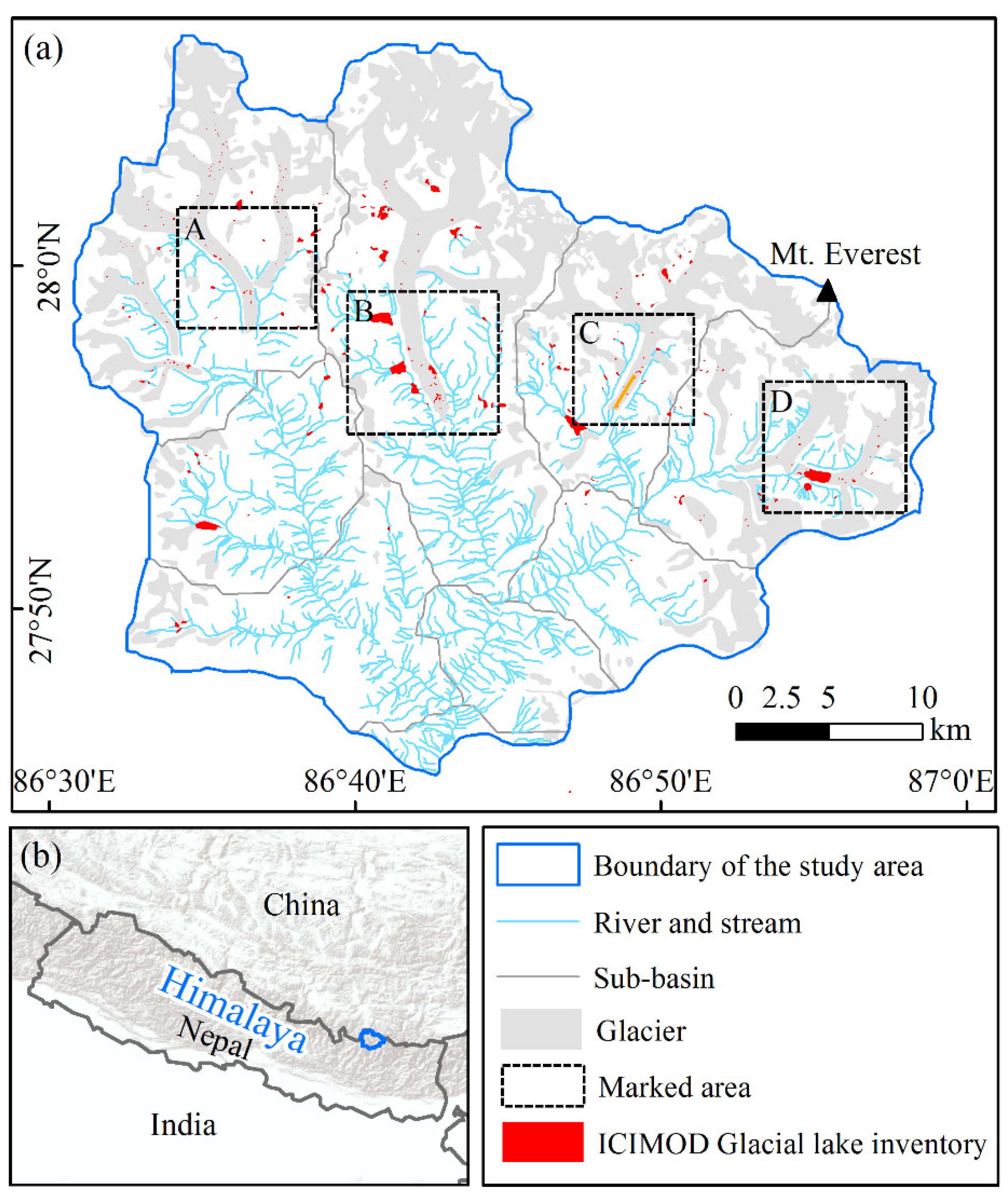
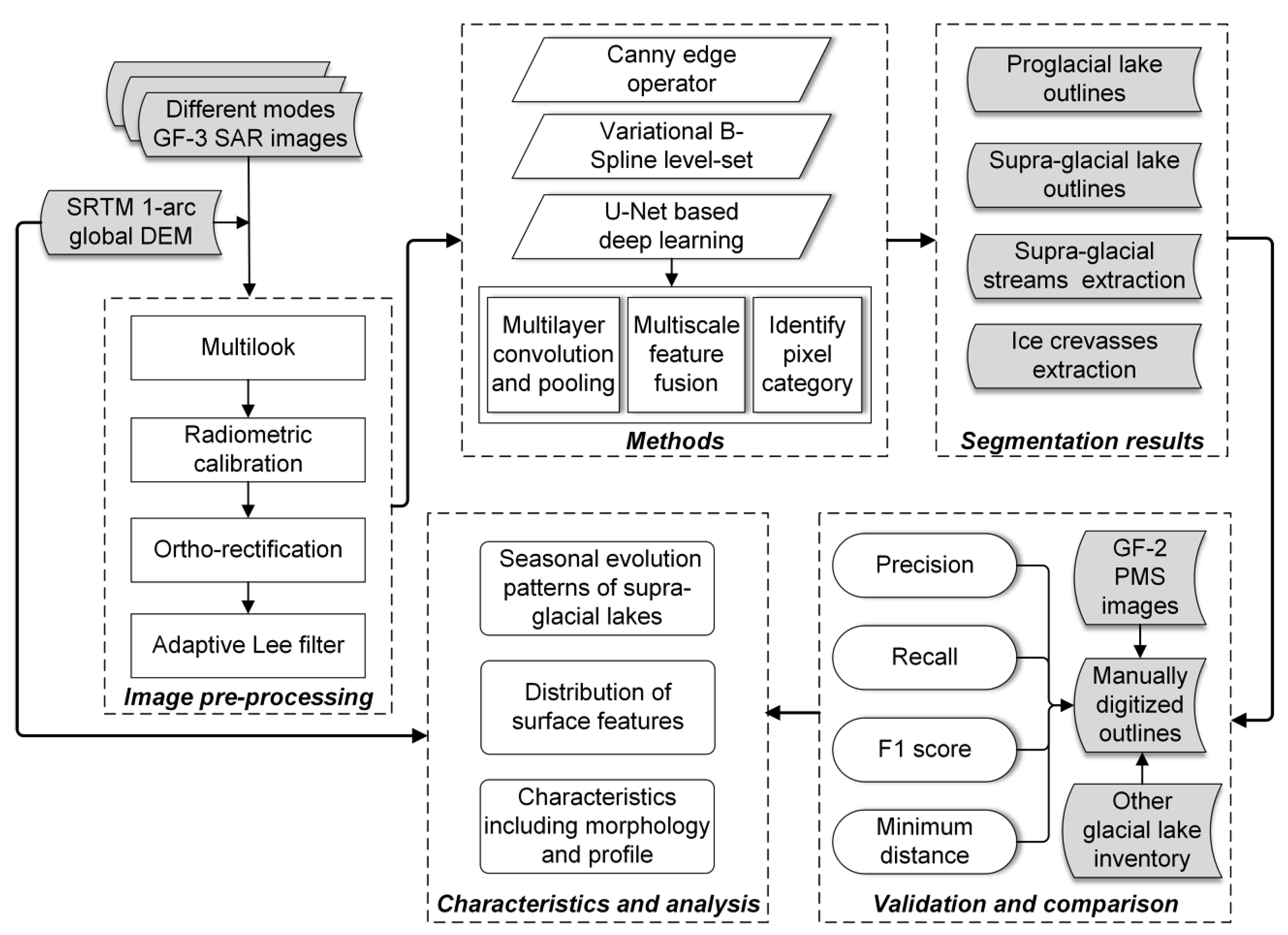
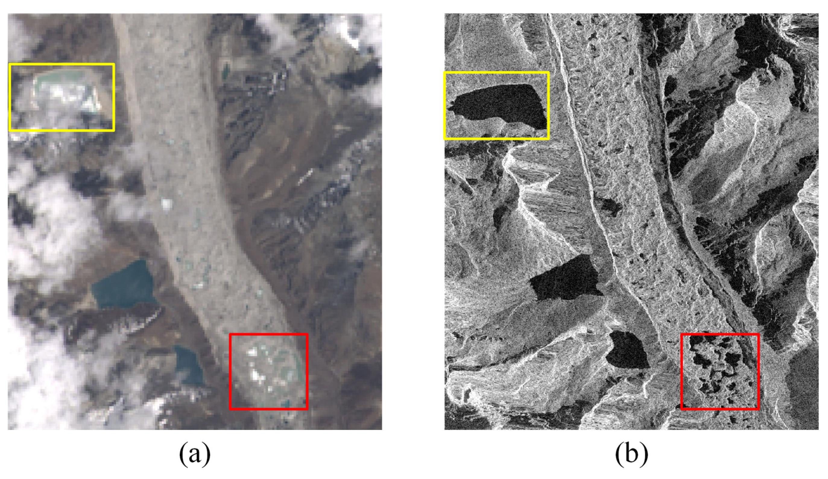
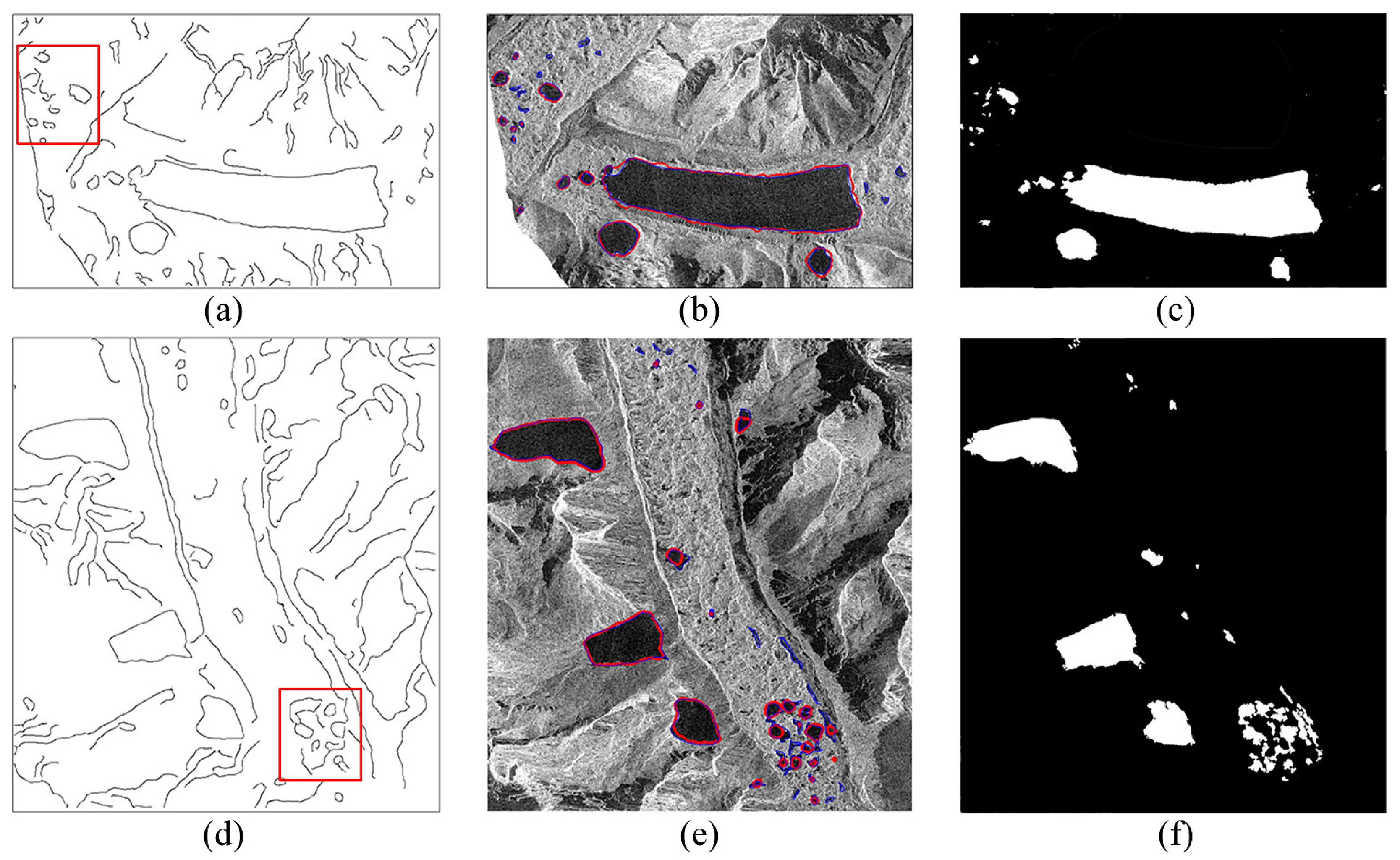
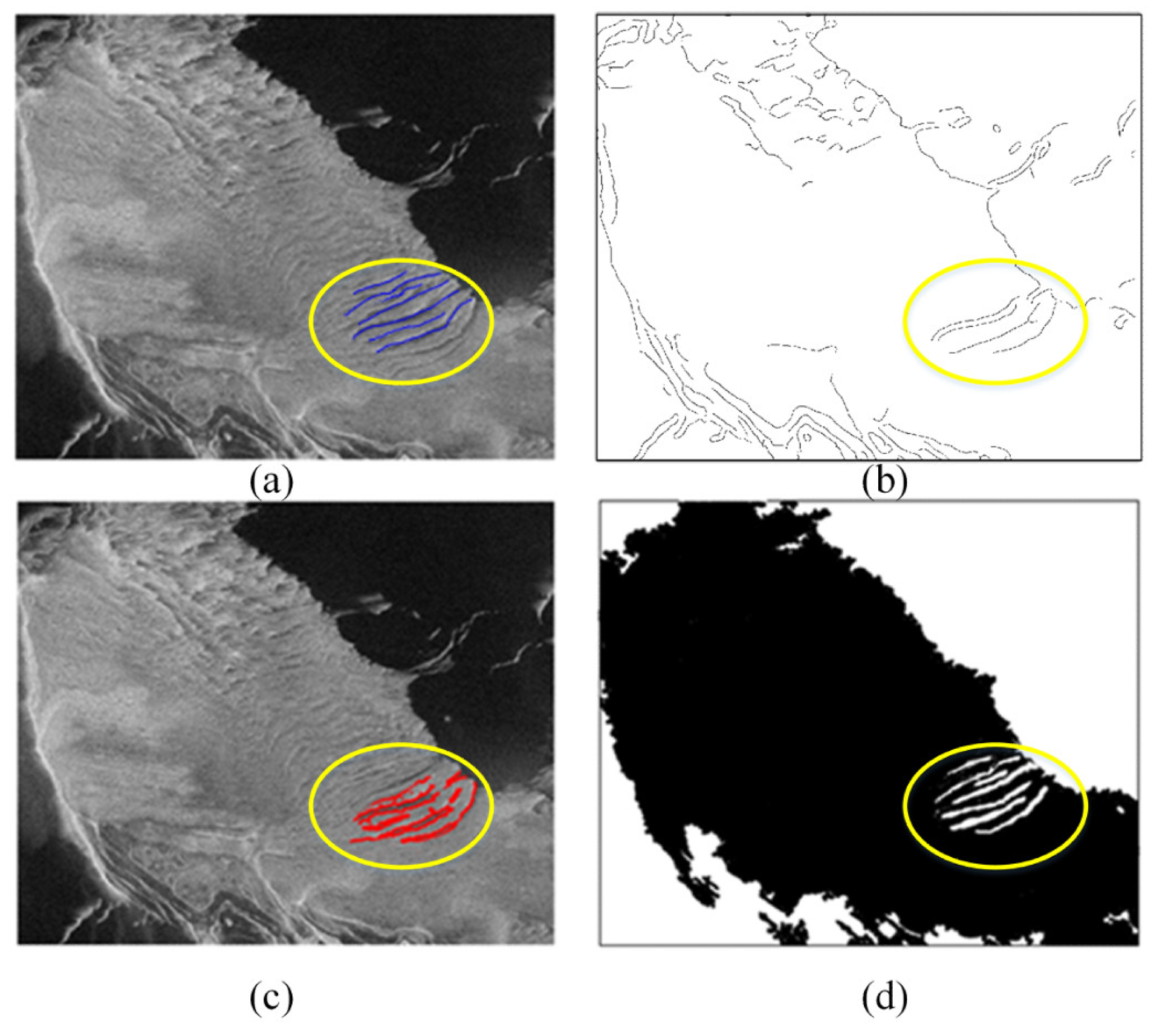
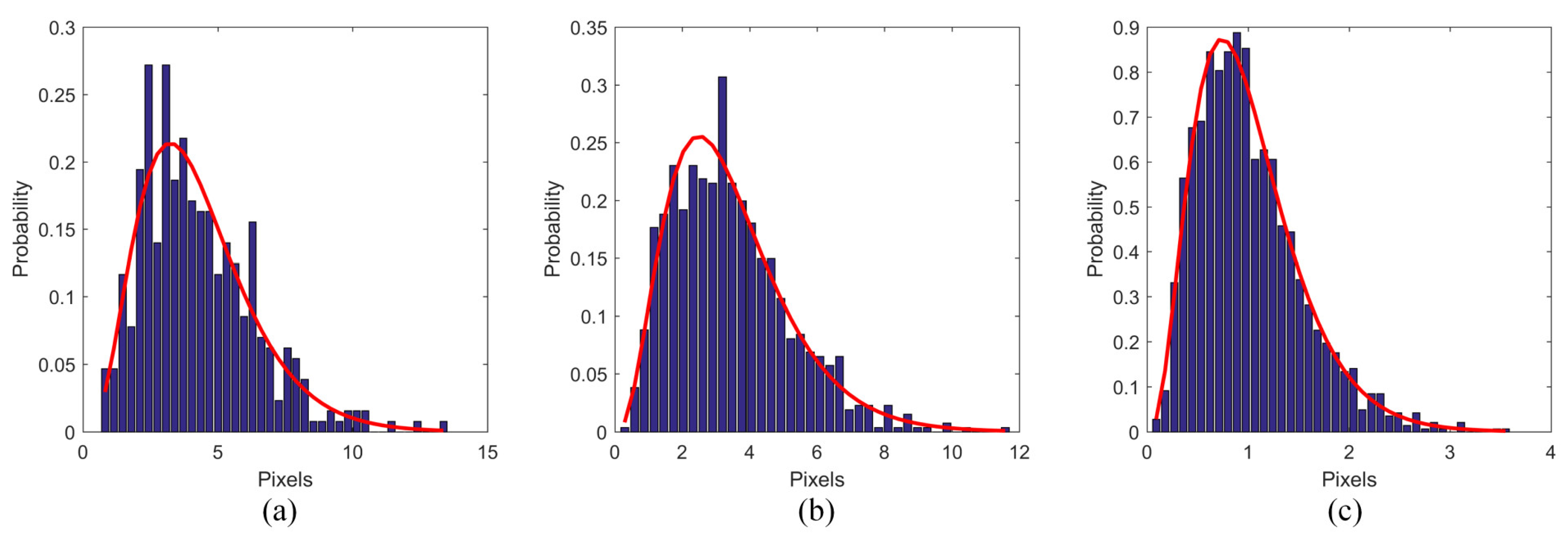
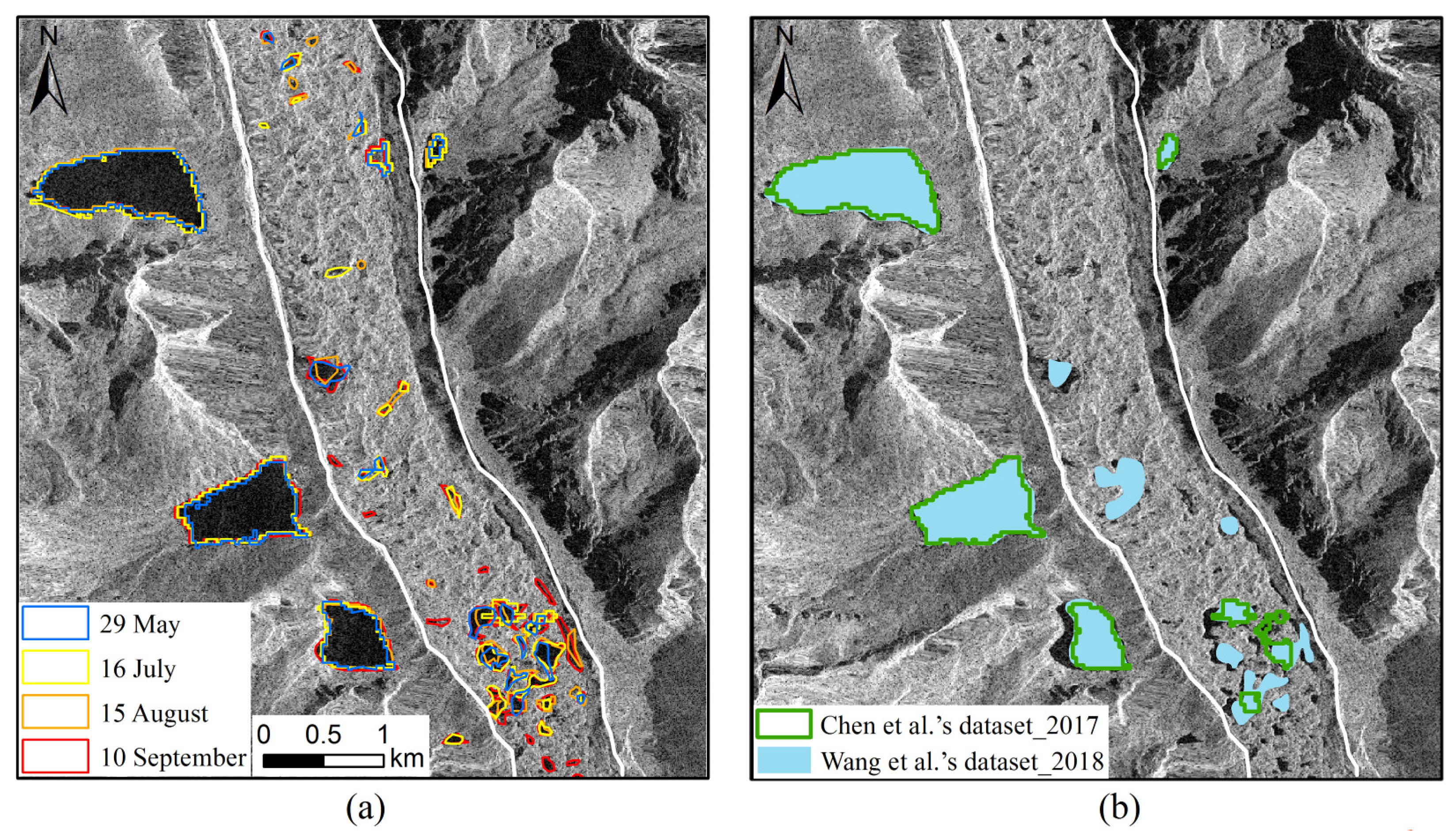
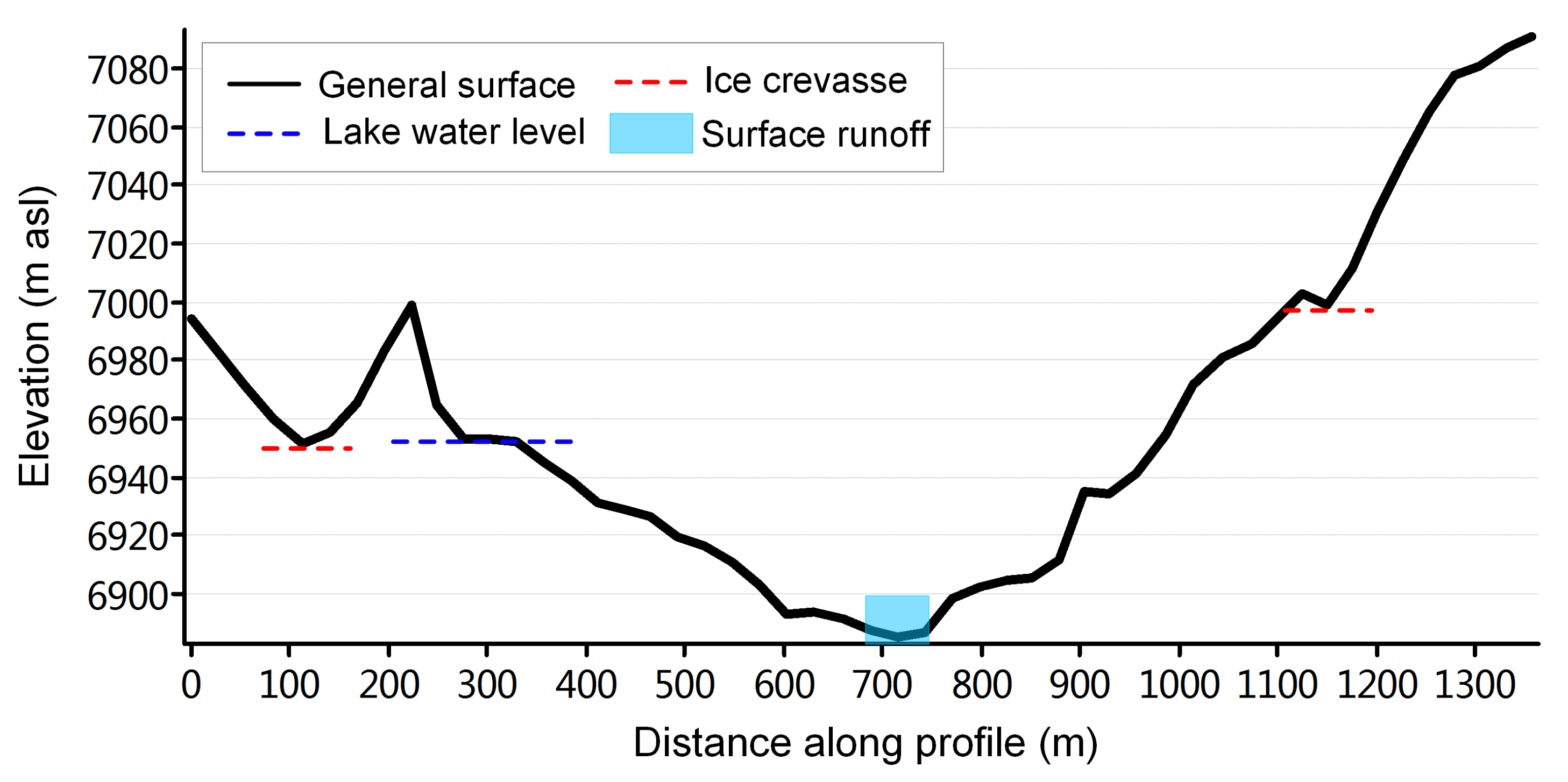
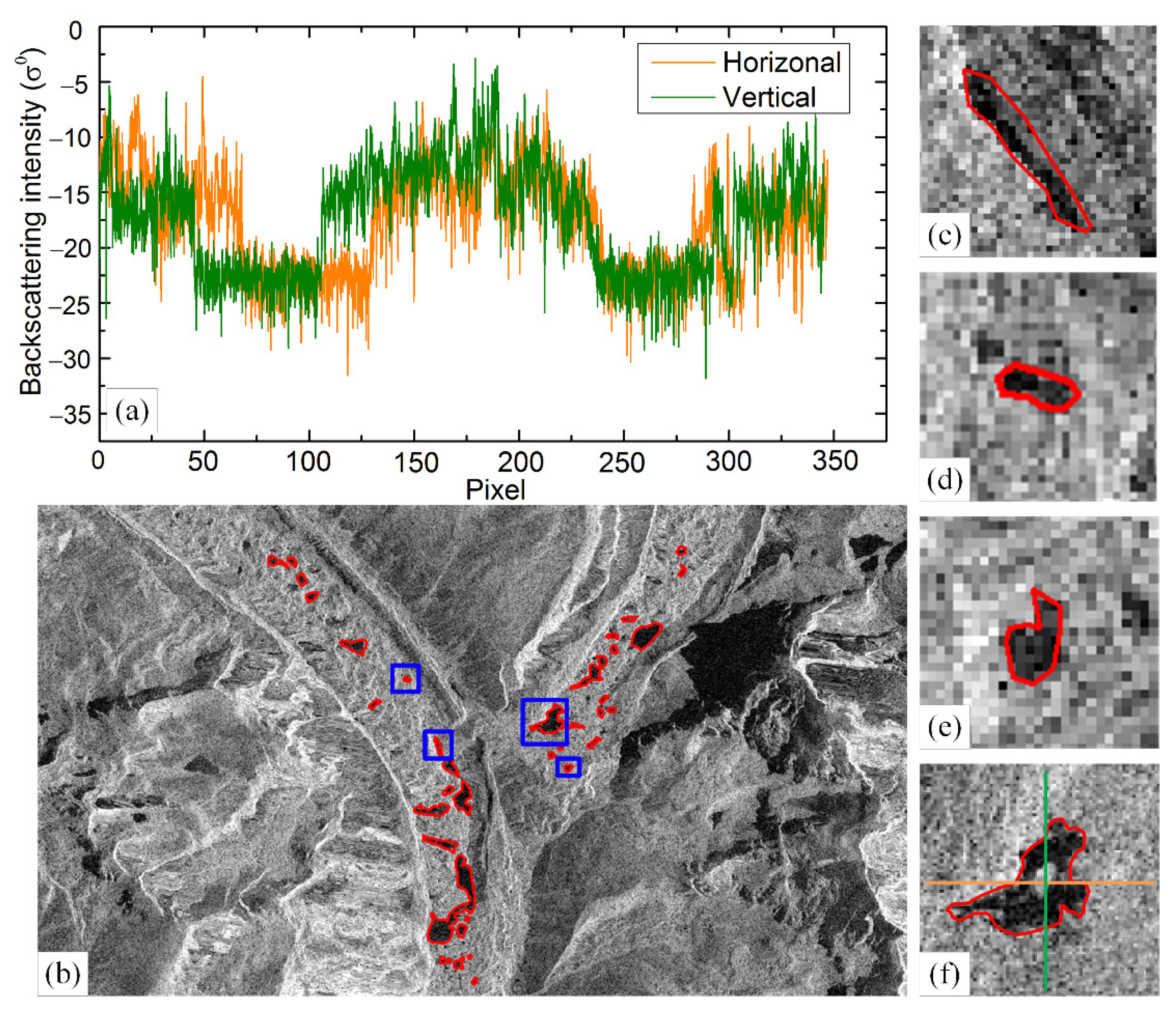
Table 1.
Summary of methods used for the segmentation of lakes and their surrounding features.
| Method Category | Method | Advantages | Disadvantages | References |
|---|---|---|---|---|
| Manual delineation | Manual delineation | High accuracy for small region | Time-consuming and labour-intensive; largely depends on the subjective experience and operational procedures | [1,7,8] |
| Edge detection | Canny edge operator | Extracts useful structural information, single edge response, and greatly reduces the amount of data | Manually defined thresholds; affected by a high degree of noise, resulting in the discontinuity of a line segment | [17] |
| Phase-congruency-based detector | Constant thresholds, not dependent on changes in image contrast and range, and can extract weak edge features completely | Seed points are manually selected; extracted edges are not completely closed | [19] | |
| Image segmentation | Thresholding segmentation | Simple and effective for small scale and homogeneous areas | Low accuracy for complex environments and large regions | [13,20,21,22,23] |
| Active-contour models | Topological variability and can be applied to all kinds of features, take full consideration of the regional heterogeneity | Complex calculation; many attempts should be made to choose optimized parameters | [12,24,25,26] | |
| Superpixel segmentation | Preserves the statistical characteristics of the image and segment image into many small homogeneous regions | Loss of important topological information of the original image | [27,28] | |
| Watershed segmentation | Fast and parallel computing, produces full boundaries | Over-segmentation problems; sensitive to the noise | [29,30] | |
| Object-oriented | Object-oriented segmentation | Fully express the semantic information between objects, and extracts feature information at different scales | Manually establishes optimal segmentation scale and appropriate classification rules | [31,32] |
| Deep learning | U-Net-based deep learning | Independent of auxiliary data and has a high degree of automation | The quality and quantity of training data are highly important | [34,35] |
Table 2.
Different satellite data used in this study.
| GF-3 SAR Image | GF-2 PMS Image | DEM | |||||||
|---|---|---|---|---|---|---|---|---|---|
| Orbit ID/ Scene ID | Image Mode | Acquisition Date (dd/mm/yyyy) | Spatial Resolution (m) | Swath Width (km) | Polarization | Path/Row | Acquisition Date (dd/mm/yyyy) | Cloud Cover (%) | |
| 020700/20 | FSII | 16/07/2020 | 10 | 100 | HH, HV | 77/170 | 17/07/2020 | 0.31 | SRTM 1-arcsecond global DEM |
| 020007/1 | SL | 29/05/2020 | 1 | 10 | HH | 78/171 | 02/06/2020 | 1.26 | |
| 021435/69 | UFS | 05/09/2020 | 3 | 30 | HH | 78/170 | 05/09/2020 | 0.83 | |
| 021507/70 | UFS | 10/09/2020 | 3 | 30 | HH | 76/171 | 10/09/2020 | 0.75 | |
| 021507/69 | UFS | 10/09/2020 | 3 | 30 | HH | 77/170 | 10/09/2020 | 2.10 | |
| 021141/26 | UFS | 15/08/2020 | 3 | 30 | HH | 76/171 | 16/08/2020 | 3.25 | |
| 021141/25 | UFS | 15/08/2020 | 3 | 30 | HH | 77/171 | 16/08/2020 | 0.58 | |
Table 3.
Performance evaluation for the three methods over all test regions.
| Method | Lake Type | Precision (%) | Recall (%) | F1 Score (%) |
|---|---|---|---|---|
| Canny edge operator | All glacial lakes | 85.30 | 81.23 | 86.50 |
| Supra-glacial lakes | 72.48 | 66.24 | 76.79 | |
| Variational B-spline level-set | All glacial lakes | 91.62 | 89.53 | 90.34 |
| Supra-glacial lakes | 88.39 | 80.12 | 85.73 | |
| U-Net-based deep learning | All glacial lakes | 98.45 | 95.82 | 96.93 |
| Supra-glacial lakes | 93.28 | 93.57 | 94.05 |
Table 4.
Changes in the number and area of glacial lakes at Ngozumpa and Khumbu Glaciers from May to September 2020.
Table 4.
Changes in the number and area of glacial lakes at Ngozumpa and Khumbu Glaciers from May to September 2020.
| Glacier | 29 May | 16 July | 15 August | 10 September | ||||
|---|---|---|---|---|---|---|---|---|
| No. | Area (km2) | No. | Area (km2) | No. | Area (km2) | No. | Area (km2) | |
| Ngozumpa | 18 | 0.22 | 31 | 0.41 | 28 | 0.32 | 36 | 0.42 |
| Khumbu | 19 | 0.19 | 28 | 0.37 | 30 | 0.35 | 38 | 0.21 |
Publisher’s Note: MDPI stays neutral with regard to jurisdictional claims in published maps and institutional affiliations. |
© 2021 by the author. Licensee MDPI, Basel, Switzerland. This article is an open access article distributed under the terms and conditions of the Creative Commons Attribution (CC BY) license (https://creativecommons.org/licenses/by/4.0/).
Share and Cite
MDPI and ACS Style
Chen, F. Comparing Methods for Segmenting Supra-Glacial Lakes and Surface Features in the Mount Everest Region of the Himalayas Using Chinese GaoFen-3 SAR Images. Remote Sens. 2021, 13, 2429. https://doi.org/10.3390/rs13132429
AMA Style
Chen F. Comparing Methods for Segmenting Supra-Glacial Lakes and Surface Features in the Mount Everest Region of the Himalayas Using Chinese GaoFen-3 SAR Images. Remote Sensing. 2021; 13(13):2429. https://doi.org/10.3390/rs13132429
Chicago/Turabian StyleChen, Fang. 2021. "Comparing Methods for Segmenting Supra-Glacial Lakes and Surface Features in the Mount Everest Region of the Himalayas Using Chinese GaoFen-3 SAR Images" Remote Sensing 13, no. 13: 2429. https://doi.org/10.3390/rs13132429
Note that from the first issue of 2016, this journal uses article numbers instead of page numbers. See further details here.