
A Constrained Markovian Diffusion Model for Controlling the Pollution Accumulation
by
 , and
, and
Beatris Adriana Escobedo-Trujillo
1,† ,
,
José Daniel López-Barrientos
2,*,† and
Javier Garrido-Meléndez
1 1
Facultad de Ingeniería, Universidad Veracruzana, Xalapa de Enriquez 91090, Mexico
2
Facultad de Ciencias Actuariales, Universidad Anáhuac México, Naucalpan de Juárez 52786, Mexico
*
Author to whom correspondence should be addressed.
†
These authors contributed equally to this work.
Mathematics 2021, 9(13), 1466; https://doi.org/10.3390/math9131466
Submission received: 19 May 2021
/
Revised: 16 June 2021
/
Accepted: 16 June 2021
/
Published: 22 June 2021
(This article belongs to the Special Issue Application of Optimal Control and Game Theory to the Problem of Resource Management)
Abstract
:This work presents a study of a finite-time horizon stochastic control problem with restrictions on both the reward and the cost functions. To this end, it uses standard dynamic programming techniques, and an extension of the classic Lagrange multipliers approach. The coefficients considered here are supposed to be unbounded, and the obtained strategies are of non-stationary closed-loop type. The driving thread of the paper is a sequence of examples on a pollution accumulation model, which is used for the purpose of showing three algorithms for the purpose of replicating the results. There, the reader can find a result on the interchangeability of limits in a Dirichlet problem.
1. Introduction
The aim of pollution accumulation models is to study the management of some goods to be consumed by a society. It is generally accepted that such consumption generates two byproducts: a social utility, and pollution. The difference between the utility and the disutility associated with the pollution is known as social welfare. The theory developed in this work enables the decision maker to find a consumption policy that maximizes an expected social welfare for the society, subject to a constraint that may represent, for example, that some costs of cleaning the environment are not to exceed some given quantity along time.
This paper deals with the problem of finding optimal controllers and values for a class of diffusions with unbounded coefficients on a finite-time horizon under the total payoff criterion subject to restrictions. It uses standard dynamic programming tools, the Lagrange multipliers approach, and a result on the interchangeability of limits in a Bellman equation. The driving thread of the paper is a sequence of examples on a pollution accumulation model, which is used for the purpose of showing how to replicate the theoretical results of the work.
The origin of the use of the optimal control theory in the context of stochastic diffusions on a finite-time horizon can be traced back to the works of Howard (see [1]), Fleming (see, for instance, [2,3,4]), Kogan (see [5]), and Puterman (cf. [6]). However, the stochastic optimization problem with constraints was attacked only in the late 90s and early 2000s, when some financial applications demanded the consideration of these models, under the hypothesis that the coefficients of all: the diffusion itself, the reward function, and the restrictions, are bounded (see, for Example [7,8,9,10]). Constrained optimal control under the discounted and ergodic criteria was studied in the seminal paper of Borkar and Ghosh (see [11]), the work of Mendoza-Pérez, Jasso-Fuentes, Prieto-Rumeau and Hernández-Lerma (see [12,13]), and the paper by Jasso-Fuentes, Escobedo-Trujillo and Mendoza-Pérez [14]. In fact, these works serve as an inspiration to pursue an extension of their research to the realm of non-stationary strategies.
Although this is not the first time that the problem of pollution accumulation has been studied from the point of view of dynamic optimization (for example, [15] uses an LQ model to describe this phenomenon, [16] deals with the average payoff in a deterministic framework, [17,18] extend the approach of the former to a stochastic context, and [19] uses a stochastic differential game against nature to characterize the situation), this paper contributes to the state-of-the-art by adding constraints to the reward function, and by taking into consideration a finite-time horizon. Moreover, this work profits from this fact by proposing a simulation scheme to test its analytic results. However, it would not be possible to find a suitable Lagrange multiplier for such simulations without the results presented in Example 3, and Theorem 2, below.
The relevance of this work lies in the applicability of its analytic results in a finite-time interval. Unlike the models under infinite-time criteria (i.e., discounted and average payoffs; and the refinements of the latter), which focus on finding optimal controllers in the set of (Markovian) stationary strategies, the criterion at hand considers as well the more general set of (Markovian) non-stationary strategies. This fact implies that the functional form of the Bellman equation includes a time-dependent term, and that the feedback controllers will depend explicitly on the time argument. Since the coefficients of the diffusions involved in this study are assumed to be unbounded, all of the points in will be attainable, and a verification result will be needed to ensure the existence of a solution to the Bellman equation that remains valid for all in , where T will be the horizon.
Significance and contributions.
- This paper presents an application of two classic tools: the Lagrange multipliers approach, and Bellman optimization in a finite horizon for diffusions with possibly unbounded coefficients. This fact represents a major technical contribution with respect to the existing literature.
- This study illustrates its results by means of the full development and implementation of an example on control of pollution accumulation. It also gives actual algorithms which can be used for the replication of the results presented along its pages.
- This work lies within the framework of dynamic optimization. However, it considers a broader class of coefficients than, for instance, [15]. As is the case of [16], it presents a pollution accumulation model. However, it focuses on a stochastic context (as in [17,18]), with the difference that the present project does so in a finite-time horizon, and with restrictions on both the reward and the cost functions.
The rest of the paper is divided as follows. The next section gives the generalities of the model under consideration, i.e., the diffusion that drives the control problem, the total payoff criterion, the restrictions on the cost and the control policies at hand. Example 1 introduces the pollution model. Section 3 deals with the actual (analytic and simulated) solution of the problem. Examples 2, 3, 4, Lemma 2, Theorem 2 and Example 5 illustrate the analytic technique and serve the purpose of comparing it with some numeric simulations. Finally, Section 4 is devoted to the presentation of the final Remarks.
This section concludes by introducing some notation for spaces of real-valued functions on an open set . The space stands for the Sobolev space consisting of all real-valued measurable functions h on such that exists for all in the weak sense, and it belongs to , where
Moreover, is the space of all real-valued continuous functions on with continuous ℓ-th partial derivative in , for , . In particular, when , stands for the space of real-valued continuous functions on . Now, is the subspace of consisting of all those functions h such that satisfies a Hölder condition with exponent , for all ; that is, there exists a constant such that
Define
The space is assumed to be endowed with the topology of . Similarly, in and .
2. Preliminaries
This work studies a finite-horizon optimal control problem with restrictions. In concrete, let be a measurable space. Let there also be an -adapted stochastic differential system of the form
where and are the drift and diffusion coefficients, respectively; and is a d-dimensional standard Brownian motion. Here, the set is a Borel set called the action (or control) set. Moreover, let be a U-valued stochastic process representing the controller’s action at each time .
Now, the profit that an agent can obtain from its activity in the system is measured with the performance index:
where r and are the running and terminal rewards, respectively; and the symbol stands for the conditional expectation of · given that , and the agent uses the sequence of controllers u.
The goal is to maximize (2) subject to a finite-horizon cost index of the operation:
where c is a running-cost rate, is a terminal cost rate function; is a running constraint-rate function, and is a terminal constraint-rate function. Observe that as the running reward-rate function r depends on the action of the controller; the running constraint-rate is independent of such variable.
The following is an assumption on the coefficients of the differential system (1).
Hypothesis (H1a).
The control set U is compact.
Hypothesis (H1b).
The drift coefficient is continuous on , and satisfies a local Lipschitz condition on , uniformly on U; that is, for each , there exists a constant such that for all
Hypothesis (H1c).
The diffusion coefficient σ satisfies a local Lipschitz condition on ; that is, for each , there exists a constant such that for all ; that is, there exists a positive constant such that for all
Hypothesis (H1d).
The matrix satisfies auniform ellipticitycondition, i.e., for some constant ,
Remark 1.
The local Lipschitz conditions on the drift and diffusion coefficients referred to in Hypothesis 1b–1c, along with the compactness of the control set U, stated in Hypothesis 1a, yield that for each , there exists a number such that
for all
For , and for all , define:
with as in Hypothesis 1d, and , representing the gradient and the Hessian matrix of h with respect to the state variable x, respectively.
The main application of this work is the pollution accumulation model. Although it will be possible to solve this problem within the realm of pure feedback strategies, this is not always the case. As a consequence, the set of actions needs to be widened.
Control Policies. Let be the family of measurable functions . A strategy , for some is called a Markov policy.
Definition 1.
Let be a measurable space, and be the family of probability measures supported on U. Arandomized policyis a family of stochastic kernels on satisfying:
- (a)
- for each and , such that and for each , is a Borel function on ; and
- (b)
- for each and , the function is a Borel-measurable in .
The set of randomized policies is denoted by Π.
Observe that every can be identified with a strategy in by means of the -valued trajectory , where represents the Dirac measure at f. When the controller operates policies , both the drift coefficient b, and the operator defined in (1) and (4), respectively, are written as
Under Hypothesis (H1a)–(H1d) and Remark 1, for each policy there exists an almost surely unique strong solution of (1), which is a Markov-Feller process. Furthermore, for each policy the operator becomes the infinitesimal generator of the dynamics (1) (for more details, see the arguments in [20] (Theorem 2.2.7)). Moreover, by the same reasoning of Theorem 4.3 in [20], for each , the associated probability measure of is absolutely continuous with respect to Lebesgue’s measure for every and . Hence, there exists a transition density function such that
for every Borel set .
Topology of relaxed controls. The set is topologized as in [21]. Such a topology renders a compact metric space, and it is determined by the following convergence criterion (see [20,21,22]).
Definition 2
(Convergence criterion). It will be said that the sequence in Πconverges to, and such convergence is denoted as , if and only if
for all , and , i.e., in the set of continuous and bounded functions on . Denoting by for each , the convergence referred to in (5) reduces to
Throughout this work, the convergence in is understood in the sense of the convergence criterion introduced in Definition 2.
The following Definition is this work’s version of the polynomial growth condition quoted in, for instance [18].
Definition 3.
Given a polynomial function of the form (with ), and , let the normed linear space be that which consists of all real-valued measurable functions ν on with finite w-norm given by
Remark 2.
- (a)
- Observe that for any function :This last inequality implies that any function satisfies the polynomial growth condition.
- (b)
- Assuming that the initial data has finite absolute moments of every order (i.e., for each )—see [23] [Theorem 4.2], gives thatwhere the constant depends on k, , and the constant is as in Hypothesis (H1b).
- (c)
- In the application developed throughout this paper, the constant initial data is considered. Then also has finite moments of every order (see Proposition 10.2.2 in [18]). Therefore,
Now, hypotheses on the reward, cost and constraint rates from (2) and (3) are stated. These are very standard, and represent an extension of the ones used in classic works, such as p. 157 in [23] (Chapter VI.3) and p. 130 in [24] (Chapter 3).
Hypothesis (H2a).
The functions are continuous, and locally Lipschitz on , uniformly on U; that is, for each , there exists a constant such that for all
Hypothesis (H2b).
and are in uniformly on U; in other words, there exists such that for all ,
Hypothesis (H2c).
The terminal reward and cost rates ; andthe running and terminal constraint rates are non-negative measurable functions which are locally Lipschitz on , i.e., for each , there exists a constant such that for all ,
For the reward and cost rates are written as
To complete this section, the main application of this work is introduced. It consists of a pollution accumulation model. This application is inspired by the one presented in [17,18], and satisfies Hypotheses 1a–1d and 2a–2c.
Example 1.
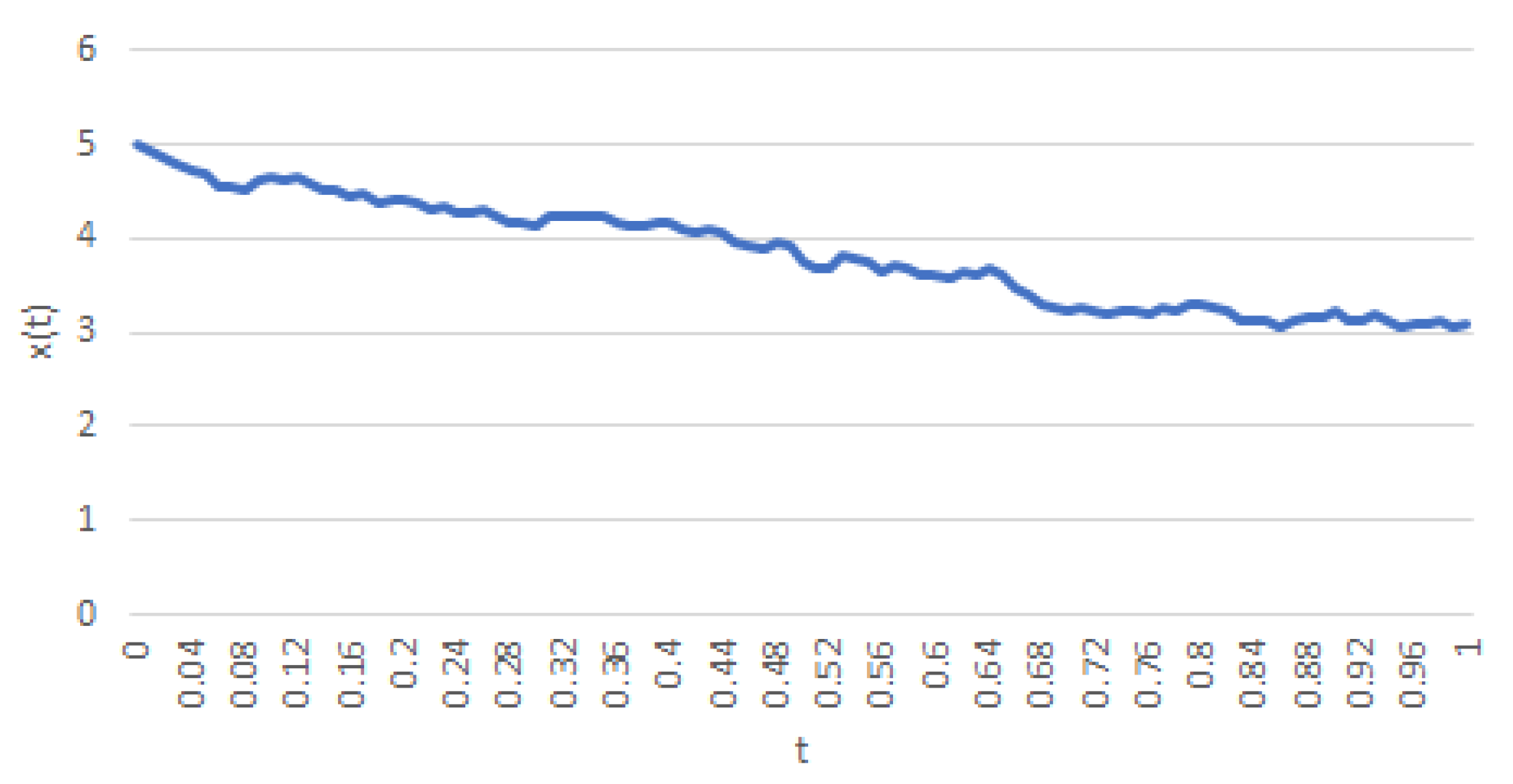
Fix the probability space , and let be a given time horizon. Consider the pollution process defined by the controlled diffusion
for , where . Here represents the consumption flow at time , and γ is certain consumption restriction imposed by, for instance worldwide protocols. Additionally, the number is the rate of pollution decay.
It is easy to see that the coefficients of (7) meet Hypothesis (H1a)–(H1c). A simple calculation yields that for any .
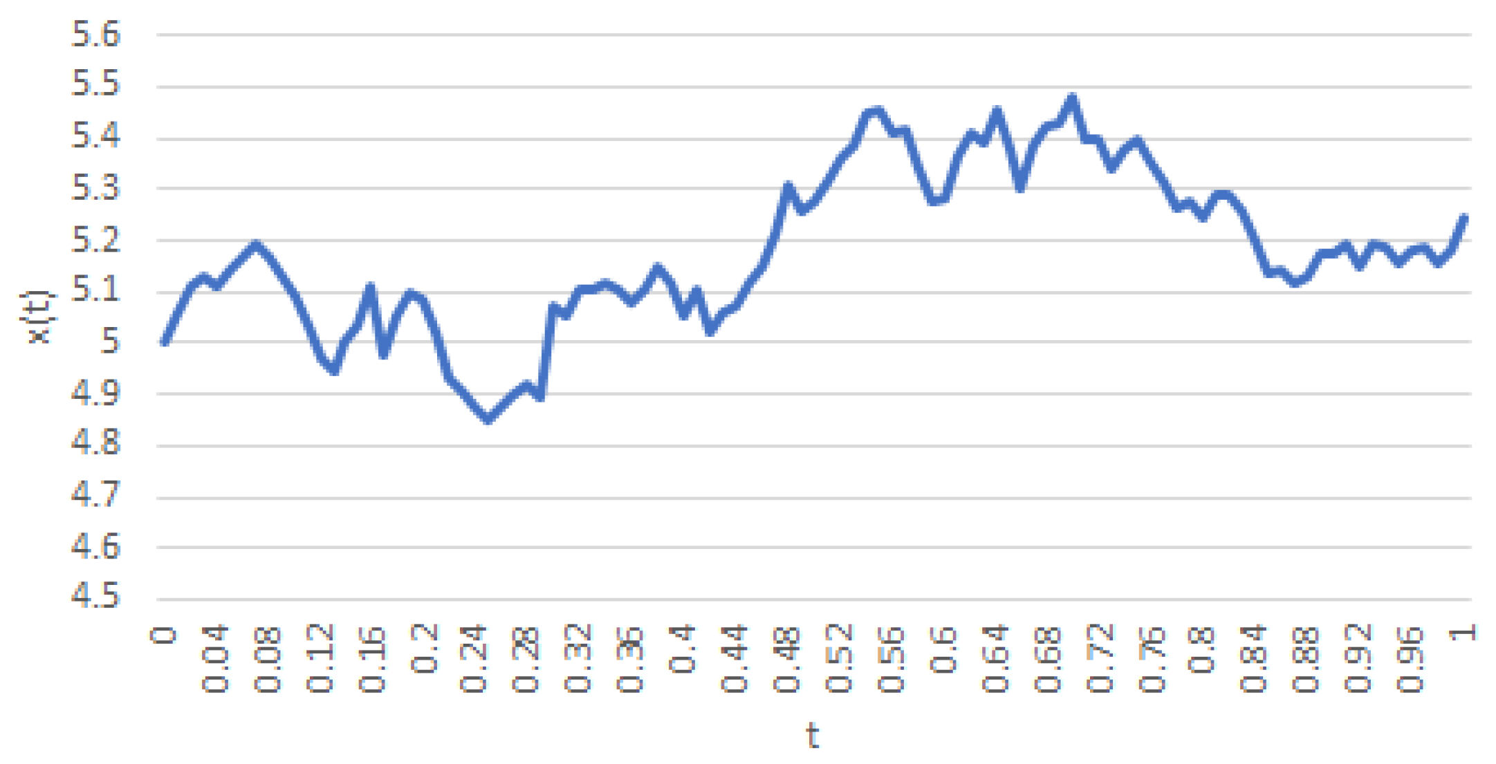
Now, a simulation of the trajectories of the Itô’s diffusion (1) is presented. To this end, the extension of Euler’s method for solving first order differential equations known asEuler-Maruyama’s method(see, for instance [25] and Chapter 1 in [26]) is used. This technique is suitable for diffusions that meet Hypothesis (H1a)–(H1d). The focus is on the comparison between Vasicek’s model for interest rates in finance (see, for instance Chapter 5 in [27]):
with , and Kawaghuchi–Morimoto’s model (7).
Let , , be the Euler-Maruyama approximations for the stochastic differential Equation (1), recursively defined by and
for all , with .
In Figure 1 and Figure 2, observe that Kawaguchi-Morimoto’s process allows one to choose a deterministic (implicit) function of t, whereas Vasicek’s series features what is known in the literature asmean reversion. The latter fact is clear from the choice of a constant parameter μ.
The polynomial function satisfies Definition 3. Please note that this function does not depend on the time argument t.
The reward-rate function used in further developments represents the social welfare, is given by , and is defined as:
where stands for the social utility of the consumption u, and stands for the social disutility (so to speak) of the pollution stock x, for fixed. It is assumed that
The cost rate function will be given by
with , and satisfying
Since the pollution stock x depends on the time variable , the functions defined in (9) and (11) also depend on this variable.
The running constraint-rate function has the form
where q is a positive constant. (Here, as with the reward and cost functions, it is assumed that x implicitly depends on t.) Theterminalconstraint, cost and reward rates will be fixed at a level of zero. It is not difficult to see that if F meets Hypothesis (H2a)–(H2c), then so do the social welfare, the cost rate and the running constraint functions.
3. A Finite-Horizon Control Problem with Constraints
This section is devoted to the introduction of the study of the finite-horizon problem with constraints.
Definition 4.
For each and thetotal expected reward, cost and constraint rates over the time interval given that are, respectively,
with and as in (6).
The proof of the next result is an extension of [28] [Proposition 3.6].
Lemma 1.
Hypothesis (H2a)–(H2c) imply that the total expected reward , the total expected cost , and the constraint rate belong to the space . In fact, for every ,
where .
Proof Proof of Lemma 1.
The proof is presented only for , for the line of reasoning is the same for and . By Hypothesis (H2b), it is known that for every ,
Now, Remark 2(b)–(c) gives that
Letting yields the result. □
For each , and , assume that the (running and terminal) constraint functions and are given, and that they satisfy Hypothesis 2c. In this way, let
To avoid trivial situations, it is assumed that this set is not empty (see Remark 3.8 in [14]). To formally introduce what is meant when talking about the maximization of (2) subject to (3), the finite-horizon problem with constraints is defined.
Definition 5.
A policy is said to be optimal for thefinite-horizon problem with constraints(FHPC) with initial state if and, in addition,
In this case, is called theT-optimal rewardfor the FHPC.
Example 2
(Example 1 continued). One intends to find a strategy that maximizes the total expected reward
subject to
That is, find such that
3.1. Lagrange Multipliers
To solve the FHPC, the Lagrange multipliers approach and the dynamic programming technique are used to transform the original FHPC into an unconstrained finite-horizon problem, parametrized by the so-named Lagrange multipliers. To do this, take and consider the new (running and terminal) reward rates
Using the same notation from (6), write
Observe also that for each , uniformly in , and . Indeed,
where , , and M as in Hypothesis (H2b).
It is natural to let, for all ,
Notice that
Example 3
(Examples 1 and 2 continued). The performance index for the FHUP is given by
Return now to Example 1, where a single trajectory of the processes (7) and (8) for certain parameters were simulated, and the policy , for (7); and , for (8). One’s aim is to compute (20) for a fixed value of , when the utility function derived from the consumption is given by , by means of Monte Carlo simulation. To this end, the following pseudocodes are presented.
Walkthrough of Algorithm 1.This pseudocode’s goal is to compute the integral inside (20).
- Line 1 initializes the process.
- Line 2 emphasizes the fact that is supposed to be given.
- Line 13 computes the integrand in (20) for the initial step.
- The while loop in lines 15–30 does the following:
- Line 31 computes the integral in (20).
Walkthrough of Algorithm 2.The purpose of this pseudocode is to compute a 95%-confidence interval for the expectation of the result of Algorithm 1 according to Monte Carlo’s method.
- Line 1 calls Algorithm 1 N times.
- Line 2 computes an average of the iterations just performed.
- Line 3 computes the sample mean of the iterations.
- The Algorithm uses the results of lines 2–3 to return the desired interval.
| Algorithm 1: Integral algorithm |
 |
Algorithm 1 receives the initial value , the step size , the time horizon T, and the parameters of the diffusion (7) (resp. (8)) to calculate the (Itô) integral inside the expectation operator in (20) when the process (7) (resp. (8)) is used; then, Algorithm 2 iterates this process and returns the average of such iteration, thus approximating the value of (20). These algorithms require a negative and constant value of the Lagrange multiplier. Later, in Example 5, a modification of Algorithm 1 that solves this situation will be proposed. For the sake of illustration, take the parameter values from Example 1 (that is , , , , , and ), and use Algorithms 1 and 2 to compute an approximation to the value of (20) when one considers the diffusion (8) (that is, the diffusion (7) with for all ). Additionally, take
| Algorithm 2: 95%-confidence interval for the expectation of an Itô’s integral using Monte Carlo’s method. |
 |
Let be any stopping time valued in , and . Should , an application of Itô’s Lemma to yields the following result.
Proposition 1.
Suppose that Hypotheses 1 and 2 are met. Fix and ; assume that there is a function satisfying:
with boundary condition Then
Notice that Proposition 1 does not assert the existence of a function that satisfies (21) (this is the purpose of Proposition 2 below). It rather motivates the definition of the finite-horizon unconstrained problem.
Definition 6.
A policy for which
is called finite-horizon optimalfor thefinite-horizon unconstrained problem(FHUP), and is referred to as thefinite-horizon optimal rewardfor the FHUP.
The first part of the following result is an extension of Proposition 1 and the verification result Theorem 3.5.2(i) in [29] to the realm of Sobolev spaces. The proof of the second part mimics that of Theorem 3.5.2(ii) in [29].
Proposition 2.
Suppose that Hypotheses 1 and 2 are met. Then:
- (i)
- For each fixed and all , the finite-horizon optimal reward defined in (23) belongs to , and verifies the total reward Hamilton-Jacobi-Bellman (HJB) equation; that is,with boundary condition . Conversely, if some function verifies (24) with boundary condition , then for all .
- (ii)
- If there exists a Markovian policy (depending on λ) that maximizes the right-hand-side of (24), i.e.,and this policy is such that the boundary condition is met as well, then this policy is a finite-horizon optimal policy for the FHUP.
Use the former result to introduce the HJB equation for the FHUP for the examples presented along the paper.
Example 4
(Examples 1–3 continued). The HJB equation for the FHUP is given by:
where ; and
According to Proposition 2, a solution of the HJB equation (25) yields the finite-horizon optimal reward and the optimal policy for the FHUP over the interval .
Now use Definition 6 and Propositions 1 and 2 to set expressions for the optimal performance index, policies, and constraint rates from the examples presented along this work.
Lemma 2
(Examples 1–4 continued). Let Λ and be the Lebesgue’s measure and the indicator function, respectively. Consider the planning horizon and assume the conditions in (7), (9)–(13) hold. Then,
- (i)
- (ii)
- DefineFor every and , the total expected reward, cost and constraint, respectively , , and ; defined in Example 2, take the form
Proof Proof of Lemma 2.
- (i)
- Start by making an informed guess of the solution of (25). NamelyObserve that , and . The substitution of these expressions in (25) yieldsThis means thatImpose the terminal condition to (34) to obtainwhere is as in (27). Now, from (35), writeTo find the supremum of the expression inside the braces, use a standard calculus argument to see that at a critical point u:Next, since by (10), , it turns out thatThen, from (37):andWith this in mind, (36) turns intoFinally, , which equalswhere stands for Lebesgue’s measure. Therefore, from (33), obtainThis proves (26)–(28). The optimality of (29) for the FHUP (20) follows from Proposition 2(ii).
- (ii)
- To see that (30) holds, use (17) to writeHere, the interchange of integrals is possible due to the finiteness of the interval , and Fubini’s rule. Now, since the solution of the controlled diffusion process (7) is given bywhere and its expected value isNow, by (29) observe that the former equals:To prove (31), use the two leftmost members in (18), and proceed as above to put:Finally, by the two rightmost members of (18), write
This proves (32).
The proof is now complete. □
3.2. From an Unconstrained Problem, to a Problem with Restrictions
This section starts with an important observation on the set of strategies which will be used.
Remark 4.
For each , define for all and
Since can be thought of as a subset of Π, Proposition 2(ii) ensures that the set is nonempty.
Lemma 3.
Let be a sequence in converging to some , and assume that there exists a sequence for each that converges to a policy . Then ; that is, π satisfies
Proof
(Proof of Lemma 3.). Recall Definition 2. Take an arbitrary sequence such that . Observe that Proposition 2 ensures that for each , satisfies:
In terms of the operator , defined in (A4), the former relation reduces to
for the special case , , , , , and constant. A verification that the hypotheses of Appendix A follows. Specifically, part (a) trivially follows from (39). Then, the focus will be on checking that part (b) of Theorem A1 is met. To do that, for some , take the ball . By [30] [Theorem 9.11], there exists a constant (depending on R) such that for a fixed :
where represents the volume of the closed ball with radius ; M and are the constants in Hypothesis (H2b), and in (14), respectively.
Notice that conditions (c) to (f) from Theorem A1 trivially hold, and that condition (g) is given as a part of the hypotheses just presented. Then, one can claim the existence of a function together with a subsequence such that uniformly in and pointwise on as and . Furthermore, satisfies:
Since the radius was arbitrary, one can extend the analysis to all of . Thus, Proposition 1 asserts that coincides with . This proves the result. □
Lemma 3 gives, in particular, the continuity of the mapping .
Lemma 4.
Assume the hypotheses of Proposition 1. Then:
- (a)
- For each fixed , , and under which :
- (b)
- The mapping is differentiable on , for any ; in fact, for each ,
Proof Proof of Lemma 4.
- (a)
- Observe that from (19), (23), and the definition of , one can assert thatOn the other hand, Proposition 2(ii) and the definition of yield the equalitySubtracting (43) from (42) yieldsApplying analogous arguments to those given in the above procedure, but taking and the policy , it is possible to obtain
- (b)
- By (15) and (16):Therefore, the continuity of follows by letting in all of the terms of (40). Now let and be fixed, and consider a sequence of negative numbers such that together with its associated sequence of policies , where for each m. From the compactness of the metric space , there exists a subsequence and such that as . From Lemma 3, belongs to , so, denote it by . By Lemma 3, the mapping is also continuous on , with . Please note that , which givesTherefore, from part (a) of this result, it turns out that the limitfor Similarly, if one considers a sequence of positive real numbers such that , it is possible to prove that there exists a subsequence such that (46) holds. This proves that is differentiable on , with derivative given by (41).
□
The following is the main result of this section. It shows how to compute optimal policies for the FHPC.
Theorem 1.
Let Hypotheses 1 and 2 hold, and consider a point fixed. Then:
- (a)
- If is a critical point of ; that is, if the derivative in (41) equals zero at , then every is optimal for the FHPC, andMoreover, is the optimal value for the FHPC which in turn coincides with . In addition,
- (b)
- Case : If satisfies ; i.e., , then this policy is optimal for the FHPC. Moreover, becomes the optimal value for the FHPC and it coincides with . Furthermore,
Proof Proof of Theorem 1.
- (a)
- Since is a critical point of , the relation (41) yields:Thus, using (19) and (49), it can be said that:Moreover, given that is in , Proposition 2(ii) and Remark 4 yieldOn the other hand, observe that for all , implying that . This last inequality, together with (19), (23), (50) and (51), leads toTherefore,Finally, by (49):yielding that is in . This fact, along with (52) and (53), gives thatthat is, is optimal for the FHPC, and coincides with the optimal reward for the FHPC.To prove (47), observe that for each and for all , Proposition 1 givesfor all , , in particular, taking in the latter expression, and observing that the second term is zero (see (49)) yieldSince was an arbitrary negative constant, then (47) holds.
- (b)
□
Theorem 2
(Examples 1–4, and Lemma 2 continued). Assume that and let fixed such that for all
and
- (a)
- (b)
- If thendefines a policy which belongs to and ; that is . Moreover, is an optimal policy for the FHPC with optimal value
Proof Proof of Theorem 2.
- (a)
- Consider from (56). Then it satisfies the following inequality tooFrom (55):Since is a strictly decreasing function, thenHence, from (29), takes the form (57). On the other hand, from Lemma 4(b), the mapping is differentiable in , withIn particular, if one considers as given by (57), and then replaces it in (31) and (32), one obtains that using the condition (54), i.e., is a critical point of the function . Thus, from Theorem 1(b), every is an optimal policy for the control problem with constraints, and , with optimal value .
- (b)
- Observe thatwhich implies that
□
Remark 5.
If the opposite condition in (54) occurs, then the existence of a critical point of the mapping implies necessarily that
In this case, every is a critical point of and is an optimal policy for the FHPC. To avoid this trivial situation, under the fact , choose γ large enough such that
Now use Theorem 2 to propose a modification of Algorithm 1 to compute the integral inside (20). Observe that it is no longer needed to include the computation of the Vasicek process (8) because the optimal values of the controllers —given by (57), and the Lagrange multipliers —given by (60)- are non-stationary along time.
Example 5
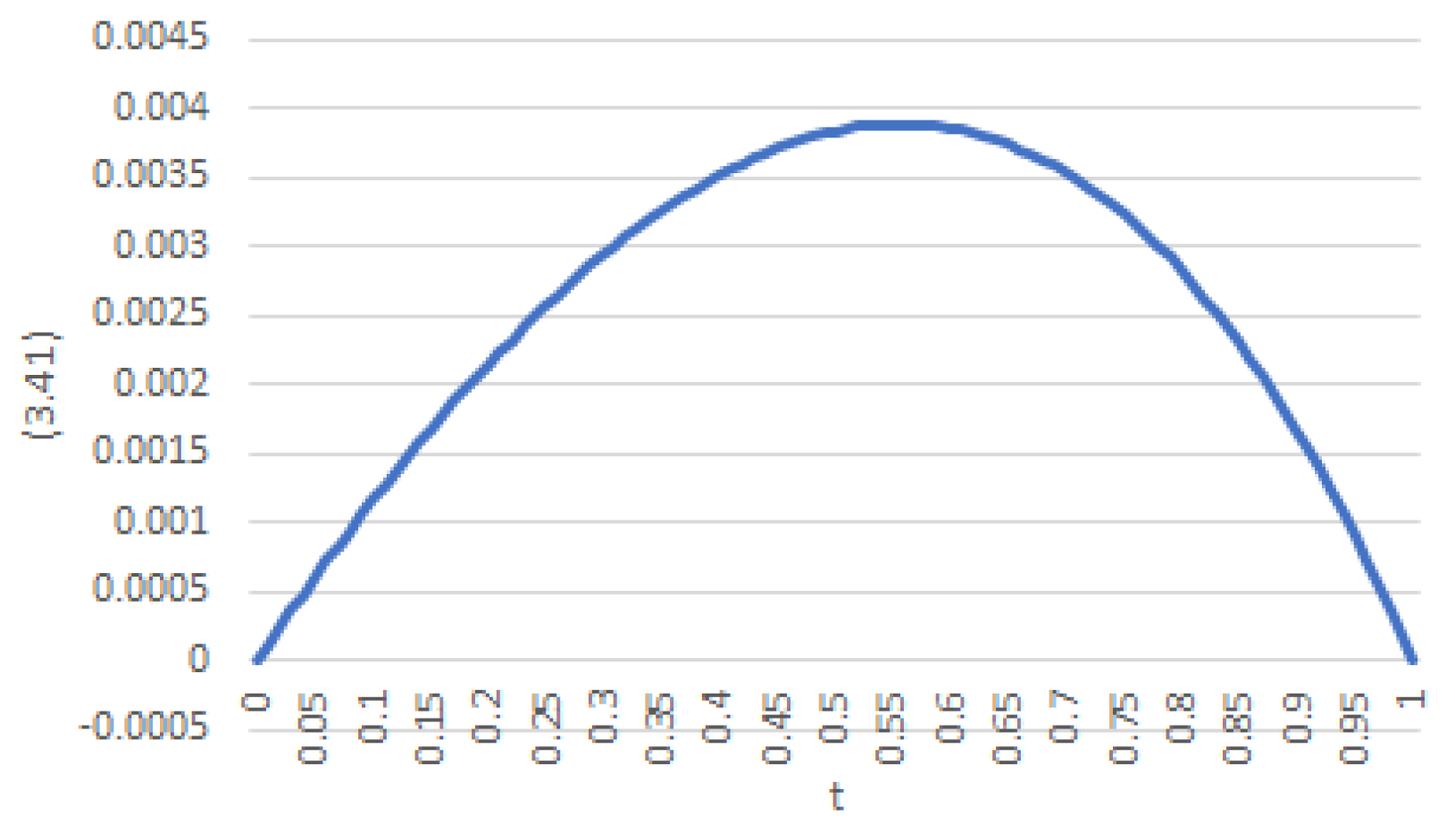
(Examples 1–4, Lemma 2, and Theorem 2 continued). Algorithms 2 and 3 can be used to compare the Monte Carlo simulations for the integral inside the expectation operator (20) with the results (formula (58)) from Theorem 2. To this end, recall from Example 1, the choice made for the parameters of (7) (that is: , , and ). In addition, choose constants that meet (12): these are , , , , and . With this configuration, condition (54) holds for all with an error of, at most (see Figure 3). With all these in mind, formula (58) in Theorem 2 yields an optimal value for the FHPC of
| Algorithm 3: Integral algorithm |
 |
The use of Algorithms 2 and 3 (with 10,000 simulations) gives optimal values for the FHUP around
4. Concluding Remarks
This paper studies a stochastic system on a finite-time horizon under the criterion of the total performance with restrictions with unbounded coefficients of all: the diffusion, the reward and the constraints. The results have been illustrated by means of a sequence of examples, a Lemma and a Theorem. The approach is based on the use of some classic dynamic programming tools, and the Lagrange multipliers technique for optimization with restrictions.
The results of this work represent a natural extension of the ones introduced in [12], to the non-stationary case. All these can also be applied to the control of pollution accumulation as presented in [17,18]. An additional contribution of this presentation is given by the optimal controllers –and objective function- for a finite-time horizon under constraints. Moreover, this work used the tools presented in [25], and the Monte Carlo simulation technique to test its analytic findings. This represents a major implication of this work concerning the current methodology for resource management and consumption when pollution has an active role. Indeed, the model presented along this paper can be used for the purpose of decision-making when the social welfare, and the cost and rewards constraints are known and parametrized.
A plausible extension of this paper could be related to looking for optimal controllers on a random horizon with a constrained performance index, in the fashion of [31].
Author Contributions
Conceptualization: B.A.E.-T. and J.D.L.-B.; methodology and software: J.D.L.-B.; investigation, validation and resources: B.A.E.-T., J.D.L.-B. and J.G.-M.; formal analysis: B.A.E.-T. and J.D.L.-B.; writing—original draft preparation: B.A.E.-T. and J.G.-M.; writing—review and editing: B.A.E.-T. and J.D.L.-B.; funding acquisition: B.A.E.-T., J.D.L.-B. and J.G.-M. All authors have read and agreed to the published version of the manuscript.
Funding
The APC was funded by Universidad Veracruzana and Universidad Anáhuac México.
Institutional Review Board Statement
Not applicable.
Informed Consent Statement
Not applicable.
Data Availability Statement
Not applicable.
Conflicts of Interest
The authors declare no conflict of interest.
Appendix A. Technical Complements
In this appendix, an extension of Theorem 5.1 from [32] to the non-stationary case with only one controller, in a finite horizon is introduced.
For , , , ; and assuming the existence of the functions , , . Now define
Furthermore, for , define
Definitions (A1)–(A4) will be used in the next couple of results.
Theorem A1.
Let be a -class bounded domain and suppose that Hypotheses 1 and 2 hold. Moreover, assume the existence of sequences , with , , satisfying that
- (a)
- , for
- (b)
- There exists a constant such that for
- (c)
- converges in to some function ε.
- (e)
- converges uniformly to some function λ.
- (f)
- .
Then, there exists a function and a sequence such that for fixed, in the norm of for as ; and for fixed, in the norm of . Moreover,
Proof of Theorem A1.
The first step is to prove the existence of a function , and a subsequence such that as weakly in , and for fixed, in the norm of for as ; and for fixed, in the norm of .
As is a reflexive space (see [33] [Theorem 3.5]), then, by [33] [Theorem 1.17], the ball
is sequentially compact for each fixed. Since , by [33] [Theorem 6.2, part III], the mapping , for is compact (and continuous too), so the subset in (A5) is relatively compact in . This ensures the existence of a function and a subsequence such that
for each . Now, since is a compact set, as weakly in , and for fixed, in the norm of for as ; and for fixed, in the norm of .
Now, it is needed to prove that
To this end, use (A1), and the triangle’s inequality, to write
Now work with the terms of the right-hand-side separately.
and
Now write
Since the mapping is continuous, Hypothesis 2b yields that for each fixed:
Since , remove the time argument from the latter expression by merely substituting the constants and by another constants. To keep the notation as straightforward as possible, this will not be done. Now, Hypothesis (H1b) gives the existence of a constant , such that Moreover, there also exists a positive constant such that
Take all of these facts, and observe that:
The boundedness of and in ; and the convergence of in the topology of relaxed controls yield that the right hand of the latter expression equals zero when . Use Theorem 2.10 in [34] to see that
This proves the result. □
References
- Howard, R. Dynamic Programming and Markov Processes; John Wiley and Sons: New York, NY, USA, 1960. [Google Scholar]
- Fleming, W.H. Some Markovian Optimization Problems. J. Math. Mech. 1963, 12, 131–140. [Google Scholar]
- Fleming, W.H. The Cauchy Problem for Degenerate Parabolic Equations. J. Math. Mech. 1964, 13, 987–1008. [Google Scholar]
- Fleming, W.H. Optimal Continuous-Parameter Stochastic Control. SIAM Rev. 1969, 11, 470–509. [Google Scholar] [CrossRef]
- Kogan, Y. On Optimal Control of a Non-Terminating Diffusion Process with Reflection. Theory Probab. Appl. 1969, 14, 496–502. [Google Scholar] [CrossRef]
- Puterman, M.L. Optimal control of diffusion processes with reflection. J. Optim. Theory Appl. 1977, 22, 103–116. [Google Scholar] [CrossRef]
- Broadie, M.; Cvitanic, J.; Soner, H.M. Optimal replication of contingent claims under portfolio constraints. Rev. Financ. Stud. 1998, 11, 59–79. [Google Scholar] [CrossRef]
- Cvitanic, J.; Pham, H.; Touzi, N. A closed form solution for the super-replication problem under transaction costs. Financ. Stoch. 1999, 3, 35–54. [Google Scholar] [CrossRef]
- Cvitanic, J.; Pham, H.; Touzi, N. Superreplication in stochastic volatility models under portfolio constraints. J. Appl. Probab. 1999, 36, 523–545. [Google Scholar] [CrossRef]
- Soner, M.; Touzi, N. Super replication under gamma constraints. SIAM J. Control Optim. 2000, 39, 73–96. [Google Scholar] [CrossRef] [Green Version]
- Borkar, V.; Ghosh, M. Controlled diffusions with constraints. J. Math. Anal. Appl. 1990, 151, 88–108. [Google Scholar] [CrossRef] [Green Version]
- Mendoza-Pérez, A.; Jasso-Fuentes, H.; Hernández-Lerma, O. The Lagrange approach to ergodic control of diffusions with cost constraints. Optimization 2015, 64, 179–196. [Google Scholar] [CrossRef]
- Prieto-Rumeau, T.; Hernández-Lerma, O. The vanishing discount approach to constrained continuous-time controlled Markov chains. Syst. Control Lett. 2010, 59, 504–509. [Google Scholar] [CrossRef]
- Jasso-Fuentes, H.; Escobedo-Trujillo, B.A.; Mendoza-Pérez, A. The Lagrange and the vanishing discount techniques to controlled diffusion with cost constraints. J. Math. Anal. Appl. 2016, 437, 999–1035. [Google Scholar] [CrossRef]
- Jiang, K.; You, D.; Li, Z.; Shi, S. A differential game approach to dynamic optimal control strategies for watershed pollution across regional boundaries under eco-compensation criterion. Ecol. Indic. 2019, 105, 229–241. [Google Scholar] [CrossRef]
- Kawaguchi, K. Optimal Control of Pollution Accumulation with Long-Run Average Welfare. Environ. Resour. Econ. 2003, 26, 457–468. [Google Scholar] [CrossRef]
- Kawaguchi, K.; Morimoto, H. Long-run average welfare in a pollution accumulation model. J. Econom. Dyn. Control 2007, 31, 703–720. [Google Scholar] [CrossRef]
- Morimoto, H. Optimal Pollution Control with Long-Run Average Criteria. In Stochastic Control and Mathematical Modeling: Applications in Economics; Encyclopedia of Mathematics and Its Applications, Cambridge University Press: Cambridge, UK, 2010; pp. 237–251. [Google Scholar] [CrossRef]
- Jasso-Fuentes, H.; López-Barrientos, J.D. On the use of stochastic differential games against nature to ergodic control problems with unknown parameters. Int. J. Control 2015, 88, 897–909. [Google Scholar] [CrossRef]
- Arapostathis, A.; Ghosh, M.K.; Borkar, V.S. Ergodic Control of Diffusion Processes; Cambridge University Press: Cambridge, UK, 2011. [Google Scholar]
- Borkar, V. A topology for Markov controls. Appl. Math. Optim. 1989, 20, 55–62. [Google Scholar] [CrossRef]
- Warga, J. Optimal Control of Differential and Functional Equations; Academic Press: New York, NY, USA, 1972. [Google Scholar]
- Fleming, W.H.; Rishel, R.W. Deterministic and Stochastic Optimal Control; Springer: Berlin/Heidelberg, Germany, 1975. [Google Scholar]
- Krylov, N.; Aries, A. Controlled Diffusion Processes; Springer: Berlin/Heidelberg, Germany, 2008. [Google Scholar]
- Higham, D. An Algorithmic Introduction to Numerical Simulation of Stochastic Differential Equations. SIAM Rev. 2001, 43, 525–546. [Google Scholar] [CrossRef]
- Hutzrnthaler, M.; Jentzen, A. Numerical Approximations of Stochastic Differential Equations with Non-Globally Lipschitz Continuous Coefficients; American Mathematical Society: Providence, RI, USA, 2015; Volume 236. [Google Scholar] [CrossRef]
- ksendal, B. Stochastic Differential Equations: An Introduction with Applications; Springer: Berlin/Heidelberg, Germany, 2003. [Google Scholar]
- Jasso-Fuentes, H.; Hernández-Lerma, O. Ergodic control, bias, and sensitive discount optimality for Markov diffusion processes. Stoch. Anal. Appl. 2009, 27, 363–385. [Google Scholar] [CrossRef]
- Pham, H. Continuous-Time Stochastic Control and Optimization with Financial Applications; Springer: Berlin/Heidelberg, Germany, 2009. [Google Scholar]
- Gilbarg, D.; Trudinger, N.S. Elliptic Partial Differential Equations of Second Order; Springer: Berlin/Heidelberg, Germany, 1998. [Google Scholar]
- López-Barrientos, J.D.; Gromova, E.V.; Miroshnichenko, E.S. Resource exploitation in a stochastic horizon under two parametric interpretations. Mathematics 2020, 8, 1081. [Google Scholar] [CrossRef]
- Alaffita-Hernández, F.A.; Escobedo-Trujillo, B.A.; López-Martínez, R. Constrained stochastic differential games with additive structure: average and discount payoffs. J. Dyn. Games 2018, 5, 109–141. [Google Scholar]
- Adams, R. Sobolev Spaces; Academic Press: New York, NY, USA, 1975. [Google Scholar]
- Folland, G. Real Analysis. Modern Techniques and Their Applications; John Wiley and Sons: New York, NY, USA, 1999. [Google Scholar]
Figure 1.
A realization of a trajectory of (7) with , , , , , and .
Figure 1.
A realization of a trajectory of (7) with , , , , , and .

Figure 2.
A realization of a trajectory of (8) with , , , , , and .
Figure 2.
A realization of a trajectory of (8) with , , , , , and .

Figure 3.
Error in the approximation of (57).
Figure 3.
Error in the approximation of (57).

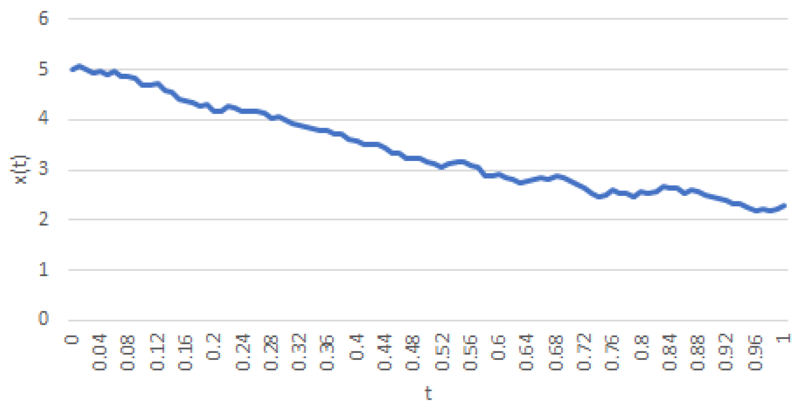
Figure 4.
A realization of a trajectory of (7) with , , , , , and .
Figure 4.
A realization of a trajectory of (7) with , , , , , and .

Publisher’s Note: MDPI stays neutral with regard to jurisdictional claims in published maps and institutional affiliations. |
© 2021 by the authors. Licensee MDPI, Basel, Switzerland. This article is an open access article distributed under the terms and conditions of the Creative Commons Attribution (CC BY) license (https://creativecommons.org/licenses/by/4.0/).
Share and Cite
MDPI and ACS Style
Escobedo-Trujillo, B.A.; López-Barrientos, J.D.; Garrido-Meléndez, J. A Constrained Markovian Diffusion Model for Controlling the Pollution Accumulation. Mathematics 2021, 9, 1466. https://doi.org/10.3390/math9131466
AMA Style
Escobedo-Trujillo BA, López-Barrientos JD, Garrido-Meléndez J. A Constrained Markovian Diffusion Model for Controlling the Pollution Accumulation. Mathematics. 2021; 9(13):1466. https://doi.org/10.3390/math9131466
Chicago/Turabian StyleEscobedo-Trujillo, Beatris Adriana, José Daniel López-Barrientos, and Javier Garrido-Meléndez. 2021. "A Constrained Markovian Diffusion Model for Controlling the Pollution Accumulation" Mathematics 9, no. 13: 1466. https://doi.org/10.3390/math9131466
Note that from the first issue of 2016, this journal uses article numbers instead of page numbers. See further details here.