
A Modelling Approach for the Assessment of Climate Change Impact on the Fungal Colonization of Historic Timber Structures


1
Department of Civil Engineering and Energy Technology, Oslo Metropolitan University—OsloMet, St. Olavs Plass 4, N-0130 Oslo, Norway
2
Finnish Meteorological Institute, Weather and Climate Change Impact Research, Erik Palménin Aukio 1, PB 503, 00101 Helsinki, Finland
*
Author to whom correspondence should be addressed.
Forests 2021, 12(7), 819; https://doi.org/10.3390/f12070819
Submission received: 28 May 2021
/
Revised: 17 June 2021
/
Accepted: 19 June 2021
/
Published: 22 June 2021
(This article belongs to the Special Issue Historical Wood: Structure, Properties and Conservation)
Abstract
:Climate change is anticipated to affect the degradation of the building materials in cultural heritage sites and buildings. For the aim of taking the necessary preventive measures, studies need to be carried out with the utmost possible precision regarding the building materials of each monument and the microclimate to which they are exposed. Within the present study, a methodology to investigate the mold risk of timber buildings is presented and applied in two historic constructions. The two case studies are located in Vestfold, Norway. Proper material properties are selected for the building elements by leveraging material properties from existing databases, measurements, and simulations of the hygrothermal performance of selected building components. Data from the REMO2015 driven by the global model MPI-ESM-LR are used in order to account for past, present, and future climate conditions. In addition, climate data from ERA5 reanalysis are used in order to assess the accuracy the MPI-ES-LR_REMO2015 model results. Whole building hygrothermal simulations are employed to calculate the temperature and the relative humidity on the timber surfaces. The transient hygrothermal condition and certain characteristics of the timber surfaces are used as inputs in the updated VTT mold model in order to predict the mold risk of certain building elements. Results show a significant increase of the mold risk of the untreated timber surfaces due to climate change. The treated surfaces have no mold risk at all. It is also observed that the most significant increase of the mold risk occurs in the north-oriented and the horizontal surfaces. It is underlined that the mold risk of the timber elements is overestimated by the MPI-ES-LR_REMO2015 model compared to ERA5 reanalysis. The importance of considering the surface temperature and humidity, and not the atmospheric temperature and humidity as boundary conditions in the mold growth model is also investigated and highlighted.
1. Introduction
Historic constructions constitute an integral part of the human cultural heritage and they play a significant role to the economies of the areas where they are located. Thus, we need to ensure their existence on a long-term horizon. Recent research underlines that an additional burden that the historic constructions have to deal with is climate change [1,2,3,4,5,6,7]. The impact of climate change on the tangible cultural heritage have been investigated in several projects, with the most known ones being the Noah’s Ark [1] and the Climate for Culture [3]. Within the Noah’s Ark project, data from climate models have been used as inputs in damage functions in order to examine the climate change impact on the deterioration of the building materials in cultural heritage sites. In the project Climate for Culture, the methodology that was followed included some additional steps in order to examine the impact of climate change on artifacts that are located in interior environments. Specifically, there were data used from climate models, material properties for the elements of the building cell, and the heat, air, and moisture (HAM) loads in the interior of certain rooms in order to calculate the air temperature and air relative humidity inside them. Then, by using appropriate standards and models describing the deterioration of the valuable tangible cultural heritage, the result of the action of certain deterioration mechanisms was investigated. The current research is conducted in the framework of the HYPERION EU project [8], which aims to create an online platform for the assessment of the resilience of historic areas by taking into account several different hazards. One of the examined hazards is climate change. In the framework of this project, specific buildings of high cultural significance are modelled in detail in order to be able to investigate their risks in a building component level. This detailed investigation is important, especially for the managers of the cultural heritage buildings, who mainly focus their conservation strategy on the material level and are also interested in examining the effectiveness of different conservation strategies. The focus of the current study is to investigate the mold risk of two timber historic buildings located in southern Norway.
In many studies, the impact of climate change on the mold risk of timber elements has been investigated [9,10,11,12] by using the biohygrothermal model [13]. In [9,10,12], the mold risk of historically significant artifacts that are made of timber was investigated, while in [11], the focus was placed on the investigation of the mold growth risk on the log walls of a historic timber construction. The biohygrothermal model accounts for the temperature and relative humidity on the surface of interest, and also for different substrate categories in order to calculate the mold growth in millimeters. One disadvantage of the biohygrothermal model is the limited number of the substrate categories that does not allow for defining of the different mold risks among different wood species, or between a rough and a planed wood surface. In addition, the biohygrothermal model does not account for the reduction of the mold risk under unfavorable conditions and, thus, it is not appropriate for the assessment of the mold risk for periods of several years. Considering the inputs, outputs, and applicability of several different mold growth models reviewed in [14,15,16], it was concluded that the assessment of the mold growth risk on the timber building elements can be most effectively employed by using the updated Technical Research Centre of Finland (VTT) mold growth model [17]. The updated VTT mold model, apart from the temperature and the relative humidity on the surface of interest, takes into account the wood species (hardwood or softwood), the type of surface (planed or rough), four different sensitivity classes, and four different material classes, according to which it can be parametrized in order to account for different final surfaces, e.g., untreated sapwood, surface treated with tar, etc. The updated VTT mold model also accounts for the decrease of the mold level during unfavorable growth periods.
The temperature and the relative humidity on both the exterior and the interior surfaces of the building components should be defined in order to be used as inputs in the mold growth model. Their calculation can be done by using whole building heat, air, and moisture (HAM) tools, given the outdoor climate, the material properties of the building components, the type of use (e.g., visitors, interior sources of moisture), and the operating heating, ventilation, and air conditioning (HVAC) systems. The HAM tools available for such applications have been reviewed in [18]. According to the conclusions of the Climate for Culture project [3], the software that are more appropriate to be used for applications related to historic buildings are the WUFI® Plus [19] and the HAMBase [20]. The studies [9,10,12,21,22,23,24,25] are relevant applications employed within the project ‘Climate for Culture’.
Then, the input material properties should be defined for the components of the buildings under investigation. Within the studies [9,10,12,21,22,23,24,25], the material properties have been selected from existing databases. In the current research, the material properties should be defined with greater accuracy. For this purpose, a methodology to select the proper material properties for the simulated building components is proposed. Within this method, material properties from existing databases, measurements, and simulations of the hygrothermal performance of selected building components are used. The hygrothermal models suitable to be used in such applications, as well as the input material properties that they take into account, have been reviewed in [26].
In addition, climate data from climate models are used in order to account for the past, present, and future conditions. The focus is to investigate the climate change impact on the mold growth of various building components and how it may vary based on the different exposure environment, i.e., differences between indoors and outdoors and differences among different orientations. Moreover, climate data from ERA5 reanalysis for the present conditions are used in order to assess the accuracy of the results deriving from the climate models. Finally, the importance of assessing the mold growth on the building components by taking into account the surface temperature and the surface relative humidity, and not the atmospheric temperature and the atmospheric relative humidity is also investigated. It should be highlighted that the calculation of the temperature and the relative humidity on the exterior and the interior surfaces of the building elements indicates the computationally demanding process of the employment of whole-building hygrothermal simulations, given the material properties of the building cell and the outdoor climate.
2. Materials and Methods
The study consists of an experimental part and numerical simulations.
The experimental part is focused on:
- Description of the case studies;
- Determination of the presence of fungal colonization in aerosol and on the material surface, and identification of the microfungi in the laboratory;
- Mapping the geometry and different building materials in the two case studies;
- Monitoring of the hygric and thermal performance of selected building elements in order to validate, on a later stage, respective numerical simulations.
The numerical simulations are focused on:
- Using measurements from the sensors, material properties from existing databases, and a one-dimensional hygrothermal simulation tool in order to select appropriate material properties for the components of the two buildings;
- Synthesis of climate files that will be used in order to assess the climate change impact on the hygric and thermal performance of the building components;
- Employment of whole building hygrothermal simulations in order to define the temperature and relative humidity on the surface of the building components (both exterior and interior) under the considered climate excitations;
- Use of a mold growth model that accounts for the transient hygrothermal conditions of the building elements in order to assess their mold risk.
At this point, it is noteworthy that the hygrothermal building simulation software WUFI® provides an extensive database with material properties relevant to the building materials of the current study. In addition, the software packages WUFI®Pro 5.3 by Fraunhofer Institute for Building Physics (IBP), Germany [27], WUFI®Plus V.3.2.0.1 by Fraunhofer IBP, Germany [28], and WUFI Mould Index VTT 2.1 by Technical Research Centre of Finland and Fraunhofer IBP, Germany [29] can be used for the one-dimensional hygrothermal simulations, whole building hygrothermal simulations, and mold risk assessment, respectively. This is the main reason why this specific software family has been selected in the current research. The WUFI® software is a numerical solver of a moisture transfer and an energy transfer equation, which are coupled. More information on the governing transport equations and the calculation procedure can be found at [30].
2.1. Experimental Part
2.1.1. Study Site
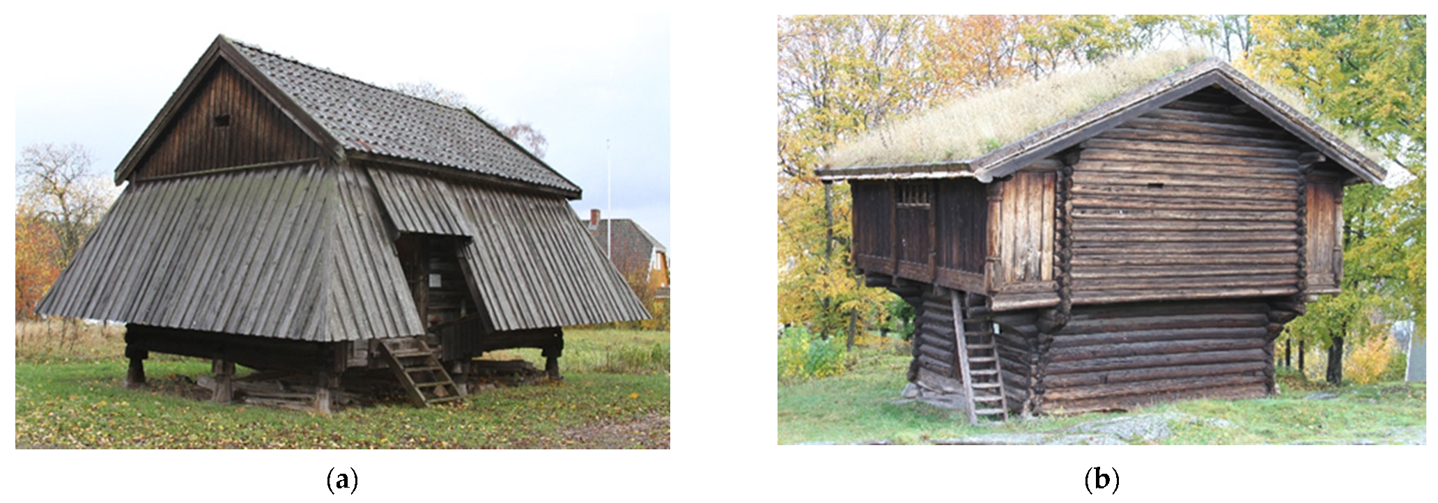
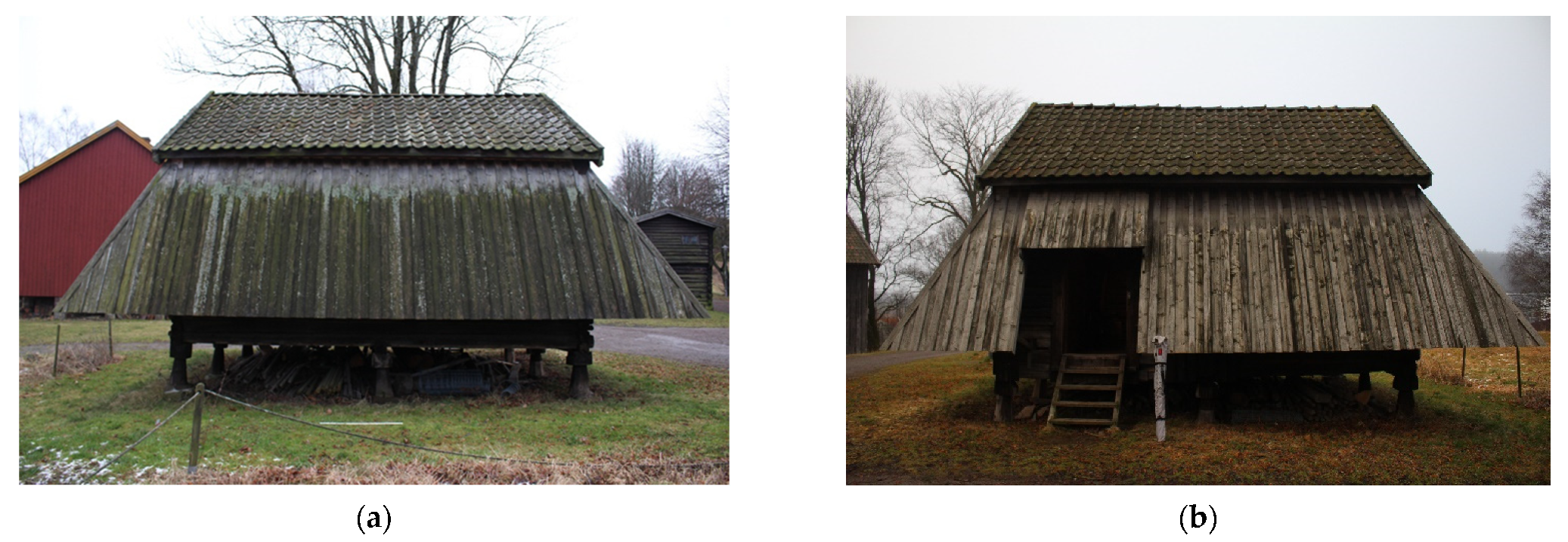
In this research, the focus has been placed in the county of Vestfold, Norway, which hosts the highest number of timber historic buildings in the country. Specifically, in the city of Tønsberg, there are several historic timber buildings which have been moved there from various regions around Vestfold, and they are currently property of the Slottsfjell museum. The effect of the buildings’ displacement on their hygrothermal performance was insignificant. That is because the climatic conditions in their former and current location—both in the county of Vestfold—are similar. In addition, the traditional techniques of wood preservation were respected in any rehabilitation project employed by the Slottsfjell museum. The two buildings selected to be investigated in the current research are the Fadum storehouse (Figure 1a), having a characteristic design that is found only in the examined area, and the Heierstad loft (Figure 1b), which is the oldest building in the area. Both buildings owe their names to the region that they originally come from.
The Fadum storehouse is a two-storey building and is dated back to 1820. In 1958, it was moved to its current location at the Slottsfjellet hill. It has a rectangular plan, with its major axis east–west oriented. Its entrance is in the southern façade. Its unique design features are the pillars or stumps upon which it stands and the shed or coating that surrounds the main body of the building. It also has openings in the eastern and western façade, both in the ground and upper floor. The stumps contribute to keeping the lower part of the construction dry, since they protect it from the ground rising damp, and they also allow the wind to flow under the main body of the construction. The coating-shed protects the outer walls from rain, wind, and solar radiation. Finally, the openings in the smaller facades of the building ensure adequate natural ventilation to its interior. The Heierstad loft is also a two-storey building. Its ground level is dated back to 1407, while its upper level was reconstructed in 1957, when the building was moved to the Slottsfjellet hill. The building is not directly based on the ground, but it stands on rocks. It has openings in its upper floor, in three out of four facades, and a turf roof that was reconstructed in 2019. The main body of both constructions is built of horizontal logs notched at the corners. The log walls are made of softwood, most likely Scotch pine (Pinus sylvestris) or Norway Spruce (Picea abies), treated with tar on their outer surface.
2.1.2. Fungi Sampling Strategy and Microscopy Analysis
Fungal growth was detected on some building components of the two constructions and, thus, it was decided to examine it thoroughly. Fungal colonization, both in aerosol and on the surface of the building elements, was investigated. Active sampling was performed outdoors, in the ground, and in the upper level of the two buildings in order to detect fungal cells and spores. A portable Surface Air System (SAS) sampler with a flow rate of 180 L/min was used for active sampling. In all sampling positions, both malt and dichloran glycerol (DG-18 without hyphen) agar were used as the growth media in the plates. The fungal colonies were counted three days after the sample collection and the fungal identification took place ten days after the sample collection. Regarding the fungal colonies on the building material surfaces, samples were collected in malt agar plates by using a pocketknife and the fungal species on them were identified in the laboratory ten days later. The morphology of fungi isolated colonies was observed by an optical microscope. In particular, conidiophores and conidia fungal structures were examined after methylene blue staining.
2.1.3. Monitoring Strategy and Sensors
The building elements of the examined constructions are made of different types of timber and have a different age. For that reason, the building components were grouped into homogeneous categories, and representative building elements from each category were selected in order to monitor their hygrothermal performance by using sensors (Figure 2). The sensors monitor the air temperature (θ) and the air relative humidity (φ) every 5 min on both sides of the building element, the moisture content inside the building element (u) every 4 h, and, in one case, the temperature inside the timber component (θtimber) every 5 min. The measurement of the temperature inside the timber prerequisites drilling a hole of 5 mm in diameter and 10 mm in depth in order to fit the sensor inside. The irreversible damage on the log wall in order to install this certain type of sensor is the reason why only one of them was used.
In more detail (Figure 2), three sensors monitoring the air temperature and the air relative humidity were placed in the Fadum storehouse. One sensor was placed in the upper floor (sensor A), the second in the ground floor (sensor C), and the third one under the coating (sensor F). Moreover, sensors monitoring the moisture content at the interior side of the south-oriented wall of the upper level (sensor B) and the ground level (sensor D) were installed. Finally, one sensor was installed to monitor the temperature inside the timber at the interior side of the south-oriented wall of the ground level (sensor E).
At the Heierstad loft, three sensors monitoring the air temperature and the air relative humidity were installed, one at the opening of the northwest façade of the upper floor (sensor G), another at the bigger room of the upper floor (sensor I), and the last one at the ground floor (sensor K). In addition, the moisture content at the interior side of the northwest-oriented log walls of the upper and ground level were monitored by the sensors H and J, respectively.
It is worth mentioning that the installation depth of the sensor monitoring the temperature inside the wood was 10 mm, and its measurements corresponded to the average temperature along the installation depth. In addition, the moisture content sensors measured the electrical resistance between two electrodes and converted it to water content units based on Equation (1). The electrodes were installed at the depth of 10 mm, and the distance between them was 20 mm. The measurements of the sensors corresponded to the average moisture content along the installation depth. The moisture content values estimated from Equation (1), together with the temperature measurements from the nearest temperature sensor, were used to calculate the temperature-corrected moisture content values with Equation (2).
The sensors installed in the Fadum storehouse have been operating since 22 November 2019, while the sensors installed in the Heierstad loft have been operating since 12 February 2020. For the aims of this study, measurements until 4 April 2020 were processed. An annual monitoring schedule would have provided a complete view of the hygrothermal performance and the moisture- and temperature-related damage on the timber components. Nevertheless, the selected period is still useful in order to assess the hygrothermal performance of the buildings and validate relevant numerical models.
where:
u: equilibrium moisture content (-);
R: electrical resistance (MΩ);
uc: temperature corrected moisture content (-);
θtimber: temperature in wood or close to the surface of wood (°C).
2.2. Numerical Simulations
2.2.1. Selection of Building Material Properties
Based on the information about the building components provided by the historic buildings’ curator (Slottsfjells museum), the planks are modern material (Figure 2) and have been replaced several times throughout the years, e.g., the planks of the coating of the Fadum storehouse were replaced in 2012 and the roof of the Heierstad loft was reconstructed in 2019. The material properties for these building elements were derived from another research on one of the two buildings [11] and coincides with the Softwood (by Fraunhofer-IBP) from the database of WUFI®Pro [27].
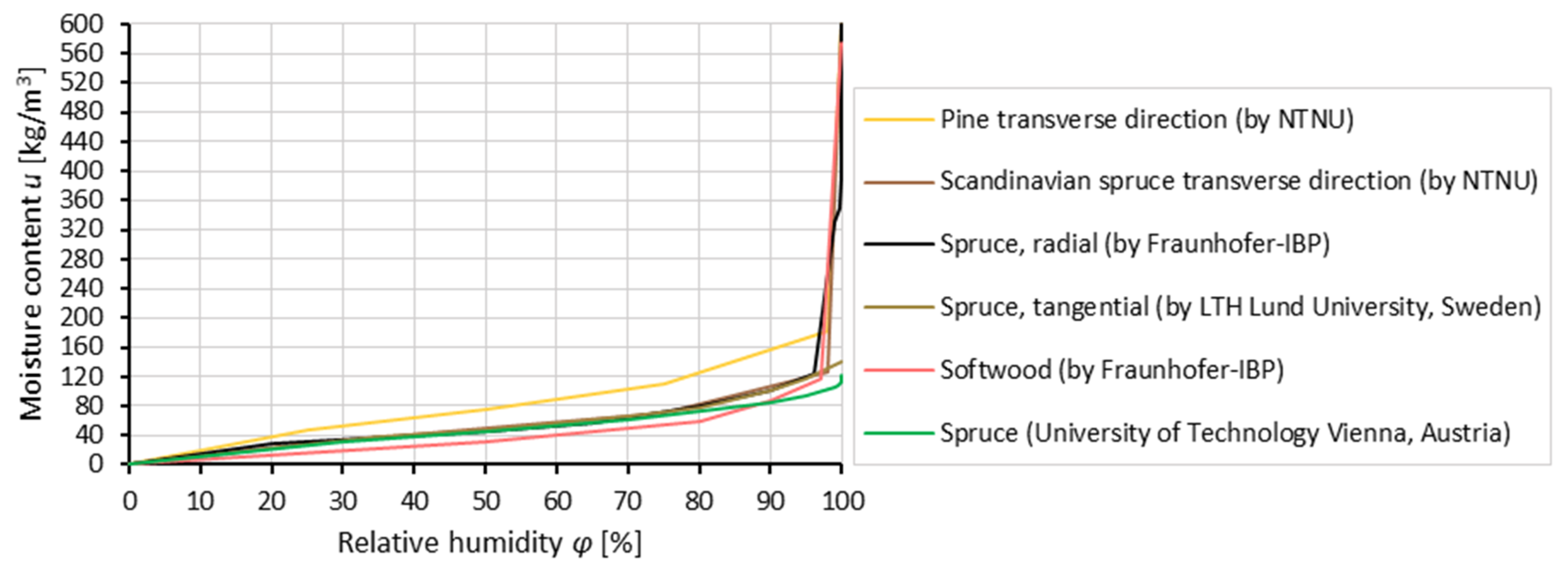
For the logs that form the main body of buildings, it is known that they have local origin and they are either Scots’ pine or Norway Spruce. In addition, all logs at the Fadum storehouse are of the same tree species and date back to 1820 (Figure 2). All logs of the ground level of the Heierstad loft are of the same tree species and are dated back to 1407 (Figure 2). Finally, all logs of the upper level of the Heierstad loft are of the same tree species and are dated back to 1957 (Figure 2). Representative logs from each category were selected in order to both monitor and simulate their hygrothermal performance (Table 1) by taking into account different sets of material properties and, finally, select the properties that provide the best fit between measurements and simulations (Equation (3)). The sets of material properties were derived from the built-in database of WUFI®Pro 5.3, and they are: (a) Softwood (by Fraunhofer-IBP, Germany), (b) Spruce, radial (by Fraunhofer-IBP, Germany), (c) Spruce, tangential (by LTH Lund University, Sweden), (d) Scandinavian spruce transverse direction (by Norwegian University of Science and Technology ‘NTNU’), (e) Pine transverse direction (by NTNU), and (f) Spruce (University of Technology Vienna, Austria). The different tree species have different hygric performance, which can be depicted in their moisture storage functions (Figure 3). For example, as can been seen in Figure 3, for an extended period of relative humidities, around 85% of the moisture content of the:
- Pine transverse direction (by NTNU) is approximately 142 kg/m3 or 27.8%, given that its bulk density (ρ) is 510 kg/m3;
- Scandinavian spruce transverse direction (by NTNU) is approximately 95 kg/m3 or 22.7%, given that ρ = 420 kg/m3;
- Spruce, radial (by Fraunhofer-IBP) is approximately 90 kg/m3 or 19.8%, given that ρ = 455 kg/m3;
- Spruce, tangential (by LTH Lund University, Sweden) is approximately 89 kg/m3 or 20.6%, given that ρ = 430 kg/m3;
- Softwood (by Fraunhofer-IBP) is approximately 74 kg/m3 or 18.5%, given that ρ = 400 kg/m3;
- Spruce (University of Technology Vienna, Austria) is approximately 79 kg/m3 or 13.1%, given that ρ = 600 kg/m3.
The 1D hygrothermal model [27] that was used to simulate the performance of the building components takes into account (i) heat transport via thermal conduction and enthalpy flow through moisture movement with phase change, (ii) vapor transport via vapor diffusion and solution diffusion, and (iii) liquid transport via capillary conduction and surface diffusion.
The agreement between measurements and simulated outputs was examined by using the goodness of fit (Equation (3)). The set of properties for which measurements and simulations had the highest fit were considered as the appropriate ones to be further used within the study.
where:
xi,meas: measured value of the hygrothermal parameter (u or θtimber) at the time step i;
xi,sim: simulated value of the hygrothermal parameter at the time step i;
N: total number of points across the studied period of time;
xmeas: the average of the measured values of the hygrothermal parameter during the studied time period.
2.2.2. Climate Data
Climate files including data about all climate parameters affecting the hygrothermal performance of the buildings were synthesized. Specifically, the following climate parameters were used:
- Air temperature θ (°C);
- Air relative humidity φ (%);
- Precipitation rr (mm);
- Wind speed ff (m/s);
- Wind direction dd (°);
- Cloud cover Nc (oktas);
- Atmospheric long-wave counter-radiation incident on a horizontal surface GLin (W/m2);
- Global short-wave radiation incident on a horizontal surface IH (W/m2);
- Diffusive short-wave radiation incident on a horizontal surface IdH (W/m2);
- Direct short-wave radiation incident on a horizontal surface IDH (W/m2).
In order to account for climate change, hourly climate data of 0.11 degrees spatial resolution were synthesized for three ten-year periods: 1960–1969 (past), 2010–2019 (current) under representative concentration pathway (RCP) 8.5, and 2060–2069 (future) under RCP8.5. The RCP8.5 represents a high-end emission scenario leading to accelerated global warming during the ongoing century [31]. The climate data used were produced with the latest hydrostatic version of the REgional MOdel REMO (version REMO2015), driven by the global model MPI-ESM-LR. The REMO [32] is a three-dimensional regional atmosphere model developed at the Max Planck Institute for Meteorology, Germany, and is currently maintained at the Climate Service Center Germany (GERICS). The MPI-ESM-LR is the low-resolution version of the Max Planck-Institute Earth System Model (MPI-ESM) [33]. The model data were acquired from the EURO-CORDEX project [34] data archive. Some additional calculations were employed in order to produce the wind direction, and diffuse and direct shortwave radiation data. Specifically, the hourly wind direction data were produced by combining files of northward and eastward wind speed having a 6 h temporal resolution and assuming constant wind direction during the whole 6 h period. In addition, the direct and diffuse shortwave radiation data were calculated by using the ENLOSS model introduced by Taesler and Andersson [35]. A brief description of the steps that were followed is provided below:
- Calculation of the solar altitude (a) and the zenith angle (z) for the sites’ position with an hourly timestep;
- Calculation of the airmass (m), given the z, by using the Young formula;
- Calculation of the saturation pressure of water vapor (pvs), given the θ, by using the relations found at [36];
- Calculation of the vapor partial pressure (pv), given the pvs and the φ;
- Calculation of the absorption of radiation by water vapor (F), given the pv and the m;
- Calculation of the intensity of direct radiation in the direction of normal (I’DN), given (i) the coefficient of turbidity (β), (ii) the spectral distribution of solar radiation outside the atmosphere i0 (λ) in the wavelength (λ) region 0.115–50 nm, (iii) the m, and (iv) the Nc;
- Calculation for each day of the year of the correction factor (ke) that takes into account the eccentricity of the Earth’s orbit around the Sun;
- Calculation of the direct normal radiation (IDN), given the F, the I’DN, and the ke;
- Calculation of the IDH, given the IDN and the a;
- Calculation of the IdH, given the IDH and the IH.
More information about each individual step can be found at [37]. By comparing climate data that derive from the same model and refer to different periods (past, present, and future), it is possible to detect the signal of climate change, i.e., quantify the change of each individual climate parameter throughout the years. In order to assess how much the modelled climate deviates from the actual one, a fourth climate file was prepared containing data from ERA5 reanalysis [38] for the period 2010–2019 (current conditions). ERA5 is the latest climate reanalysis produced by the European Centre for Medium-Range Weather Forecasts (ECMWF). Climate reanalyses combine past observations with models to generate consistent time series of multiple climate variables. The ERA5 data have been used because there were no applicable observations available near the study site for many of the parameters that should be taken into account. The spatial resolution of the ERA5 data is 0.25 degrees. The climate data from ERA5 are representative of the study site, given the minor topographic differences within the grid cell in ERA5, which includes the study site.
Once again, not all climate parameters that were needed could be directly downloaded. Relative humidity is not archived directly in ERA datasets, but the archive contains near-surface temperature (θ) and dew point temperature (θd), from which the relative humidity can be calculated from the equation:
where es is the saturation pressure, defined with respect to water for temperatures over 0 °C and ice for temperatures below 0 °C as described in [36].
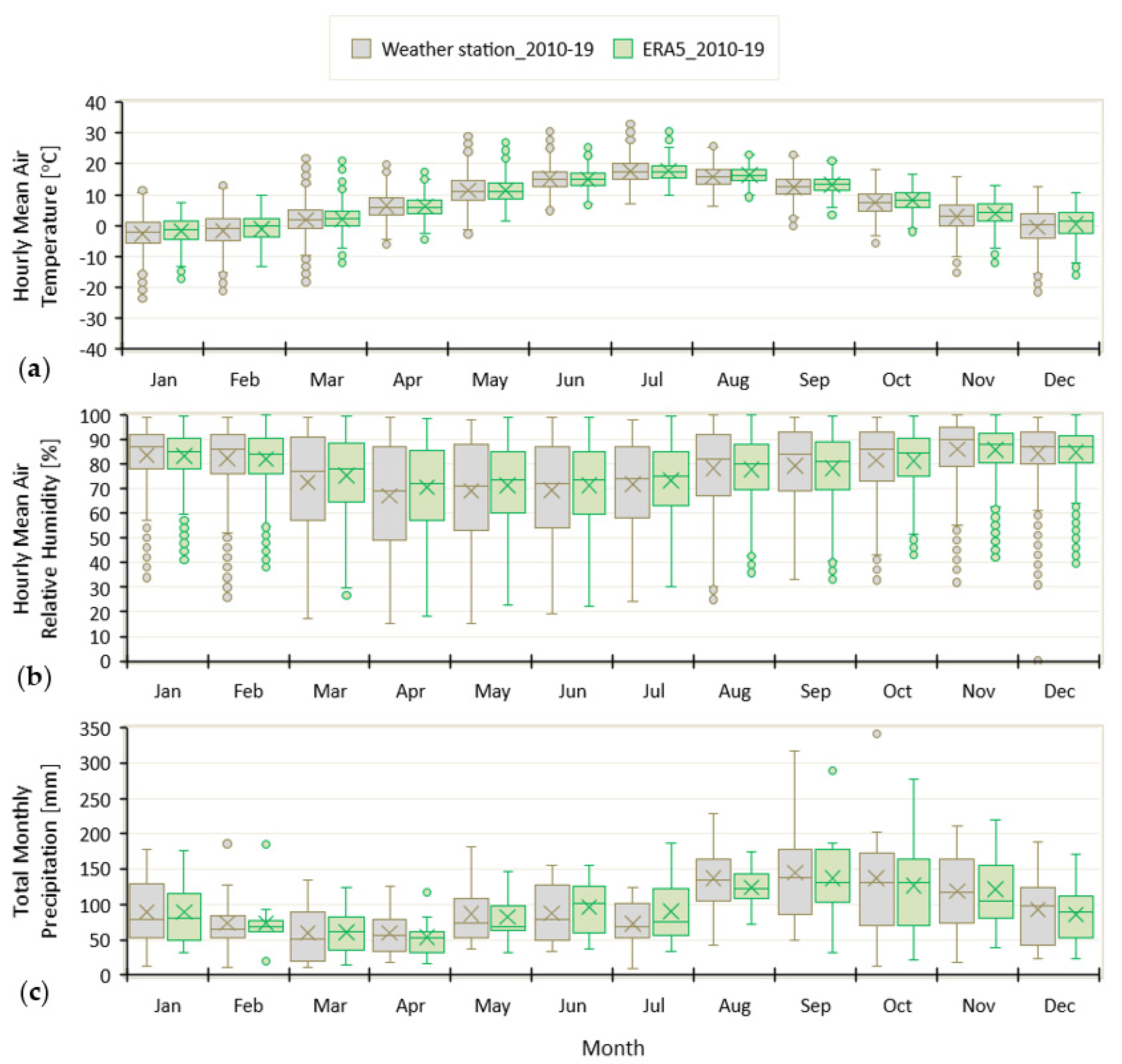
A comparison between air temperature, air relative humidity, and precipitation data derived from a weather station 5 km from the study site [39] and ERA5 reanalysis is presented in Figure 4a–c, respectively. It is verified that the data derived from ERA5 reanalysis can well describe the climate conditions in the study site. The most notable difference seems to be that the coldest temperatures are warmer in ERA5 in each month, but particularly in winter.
2.2.3. Whole-Building Hygrothermal Simulations
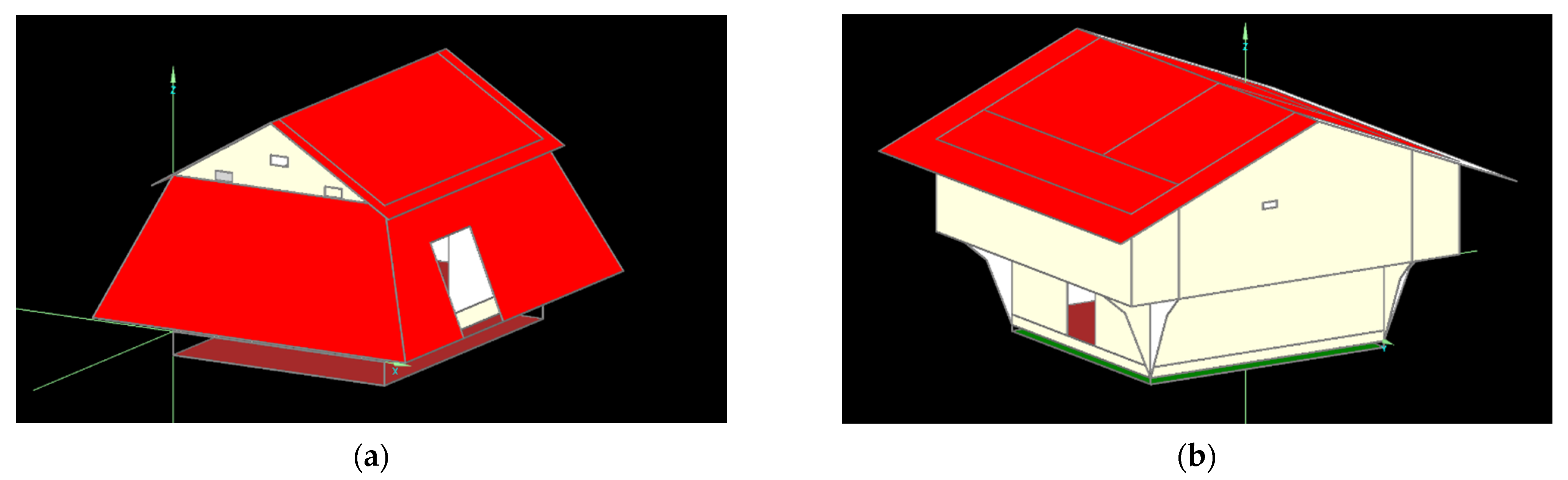
The selected material properties of the building components and the prepared climate data were used as an input in whole-building hygrothermal simulations using the software WUFI® Plus V.3.2.0.1 [28] (Figure 5). Within the employed models, the heat transport mechanisms that were taken into account were: thermal conduction, enthalpy flow through moisture movement with phase change, short-wave solar radiation, and night-time long-wave radiation cooling. The vapor transport mechanisms that were taken into account included vapor diffusion and solution diffusion. The considered liquid transport mechanisms were capillary conduction and surface diffusion. Moreover, the employed models incorporated calculations of explicit radiation balance on external surfaces shading calculations with hourly time step, wind dependent heat transfer on external surfaces, rain load calculation on external surfaces, and air flow calculation.
The buildings have no HVAC systems or transparent components. Within the airflow model the openings of the two buildings were modelled as orifices. Special attention was paid to consider within the simulations that the buildings are not directly based on the ground, but there is free air flow down below them. For that purpose, an additional zone was considered under the buildings which has the same length and width as the ground floor of each construction, and a height of 50 cm in the case of the Fadum store house and 30 cm in the case of the Heierstad loft. All vertical sides of this zone were considered as orifices within the simulations.
2.2.4. Mold Growth Model
In the current study, the WUFI Mold Index VTT 2.1 software [29] was used to calculate the mold growth on the building components according to the updated VTT mold model [17]. The updated VTT model is an empirical mold growth prediction model, which is based on regression analysis of a set of measured data [40,41]. The mold growth development is expressed by the mold index (M), which can range between 0 and 6 (Table 2). The mold index can be used as a design criterion, e.g., often M = 1 is defined as the maximum tolerable value, given that the germination process starts from the particular point.
Compared to the other mold growth models, the features of the updated VTT mold model that render it more appropriate for the aims of the current research are the following:
- Accounts for surface temperature, surface relative humidity, different types and qualities of the substrate timber;
- Estimation of growth and not just an indication of start;
- Decrease of mold level during unfavorable growth periods;
- Appropriate for application to extended periods of time (10-year periods in the current research).
The mold growth intensity in the updated VTT mold model is based on Equation (5) [17]:
where:
M: mold index (-)
t: time (h). The numerical simulation carried out using one-hour time steps (climate data intervals).
θ: temperature (°C)
φ: relative humidity (%)
W: coefficient that depends on the timber species. It is equal to 1 for hardwood and 0 for softwood and nontimber materials.
SQ: coefficient that depends on surface quality. It is equal to 1 for rough surfaces and 0 for planed surfaces and nontimber materials.
k1: coefficient that expresses the intensity of the mold growth and depends on the growth level. It is used to scale the equation for different substrate materials, e.g., a surface treated with tar and an untreated sapwood surface.
k2: coefficient to limit the growth to a maximum possible index level. It is also used to scale the equation for different substrate materials, and is calculated by Equation (6):
where:
Mmax: the maximum mold index on a specific substrate material, given by Equation (7):
where:
A, B, C: coefficients that have been determined experimentally and categorized into four sensitivity classes by [17], and they are dependent on the substrate material.
φcrit: The lowest relative humidity value where mold growth is possible when the material is exposed to it for a long enough period, and it is given by (Equation (8)):
where φmin is 80% for wood-based products and 85% for materials that are more resistant to mold growth, e.g., the surfaces treated with tar in the case studies of the current research.
The updated VTT mold model takes into account the decrease in the mold index level when the conditions (relative humidity or temperature) are outside the favorable conditions for mold growth. For this reason, the mold decline intensity for a reference material (re-sawn pine wood) is first calculated, and then multiplied by an appropriate scaling factor Cmat to adjust the mold decline intensity to the actual substrate material. More details about the updated VTT mold model can be found at [17].
As can be seen in Table 3, the model was parametrized accordingly in order to account for all different types of surfaces existing in the two case studies.
3. Results and Discussion
3.1. Mapping and Identification of Fungi
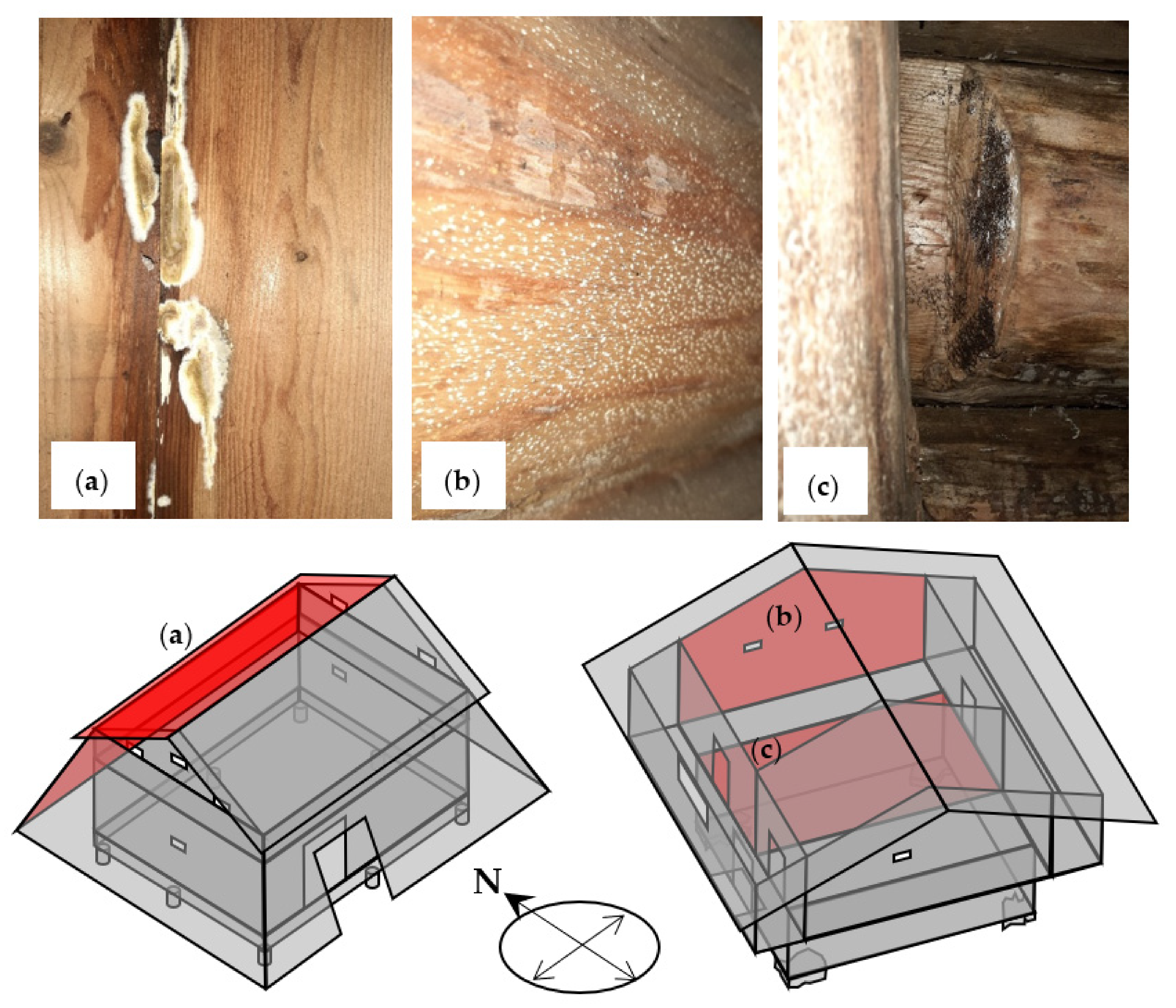
The exterior side of the building components that is treated with tar was not colonized by mold. In contrast, at the untreated planks of the coating/shed of the Fadum storehouse colonization was observed. As can be seen in Figure 6, the north-oriented side of the coating was the most aggravated. Moreover, fungal growth was detected at the interior of the two buildings. In the Fadum storehouse, brown-rot fungi (Coniophora puteana) was detected in the north-oriented side of both the roof and the coating (Figure 7a). The fungus was identified based on its fruiting body. Coniophora puteana is a wood-destroying fungus that breaks down the hemicellulose and cellulose [42]. The rotting fungus grew in positions with leaks in which the rainwater had penetrated. The infected building elements were untreated planks. These planks were replaced immediately by the historic buildings’ curator. In the Heierstad loft, fungal growth was detected at the inner side of the northeast-oriented wall of the upper level and on the ceiling of the ground floor (Figure 7). The infected surfaces were untreated logs.
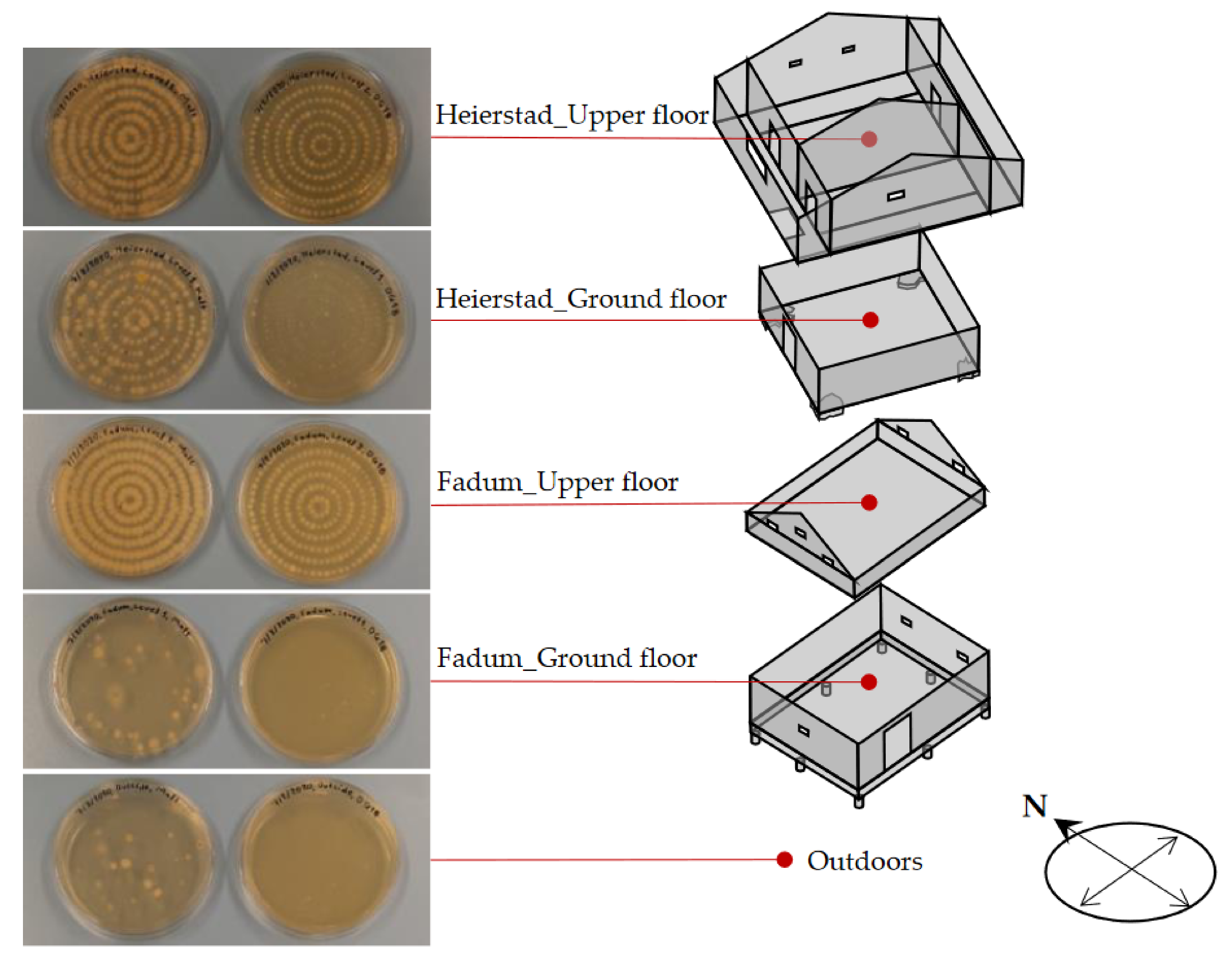
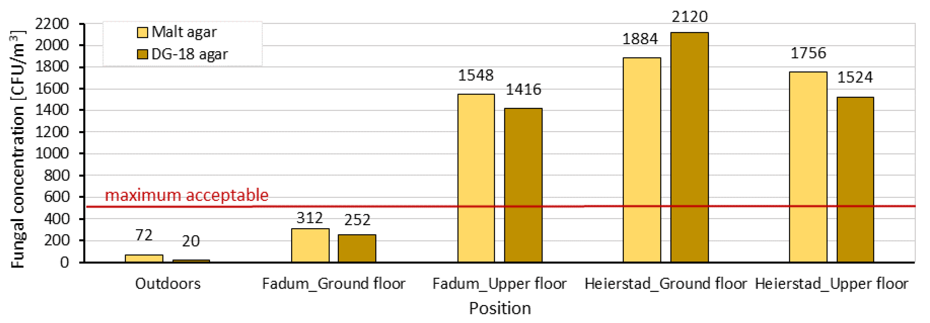
Apart from the fungi grown on the building components, samples of airborne fungal spores were also collected. In Figure 8, the position from which the aerosol samples were collected, as well as the fungi colonies grown three days after the samples collection, are shown. As has already been mentioned in Section 2.1.2, two different growth media were used in the plates. This is because some species of fungi grow favorably on malt agar, while others on DG-18 agar. Moreover, quantitative microbial concentrations were estimated for the culturable fungi colonies as colony forming units per air volume (CFU/m3) (Figure 9). As can be seen in Figure 8 and Figure 9, the smallest fungal concertation was observed outdoors. According to the same figures, in the ground level of the Fadum storehouse, the concertation of the airborne fungal spores was at acceptable levels, with values lower than 500 CFU/m3, which is the threshold defined by the World Health Organization (WHO) for noncontaminated indoor air [43]. On the upper level of the Fadum storehouse, on the ground level of the Heierstad loft, and on the upper level of the Heierstad loft, the concentration of the airborne fungal spores was extremely high, exceeding by far the maximum acceptable limit of the WHO (Figure 9).
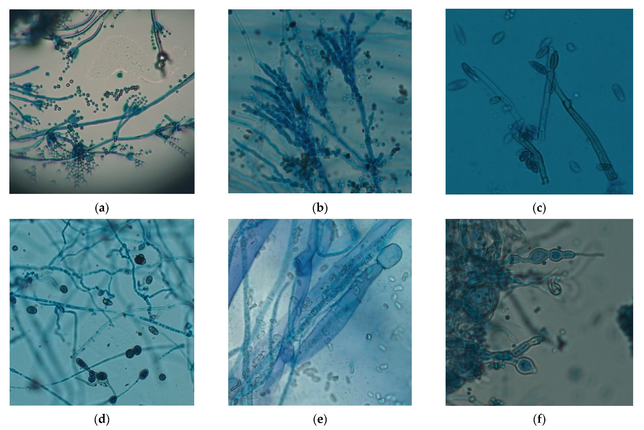
In addition, identification of microfungi grown on the plates was performed by using optical microscopy (Figure 10). In Table 4, the microfungi species found in each of the two buildings are presented. The identified microfungi (Figure 10 and Table 4) in the concentrations that were found (Figure 8) can cause irritation of the eyes and respiratory tract, headache, drowsiness, skin rash, and itching of the skin, or even allergies and more adverse human diseases [44].
It was suggested to the administrators of the historic timber buildings (i) to clean the rooms of the two buildings in order to remove the dust and organic materials that constitute proper medium for the spores to germinate, (ii) to open the doors of the two buildings during the working hours of the museum for better natural ventilation, and (iii) temporarily to not use the Heierstad loft and the upper level of the Fadum storehouse, since they constitute a threat for human health due to contaminated indoor air. A systematic air sampling strategy was also proposed in order to monitor the indoor air quality and adjust the measures that should be taken accordingly. Finally, it was highlighted that, in case of rot-fungi detection, the infected building element should be replaced immediately.
3.2. Material Selection, Measured and Simulated Hygrothermal Performance
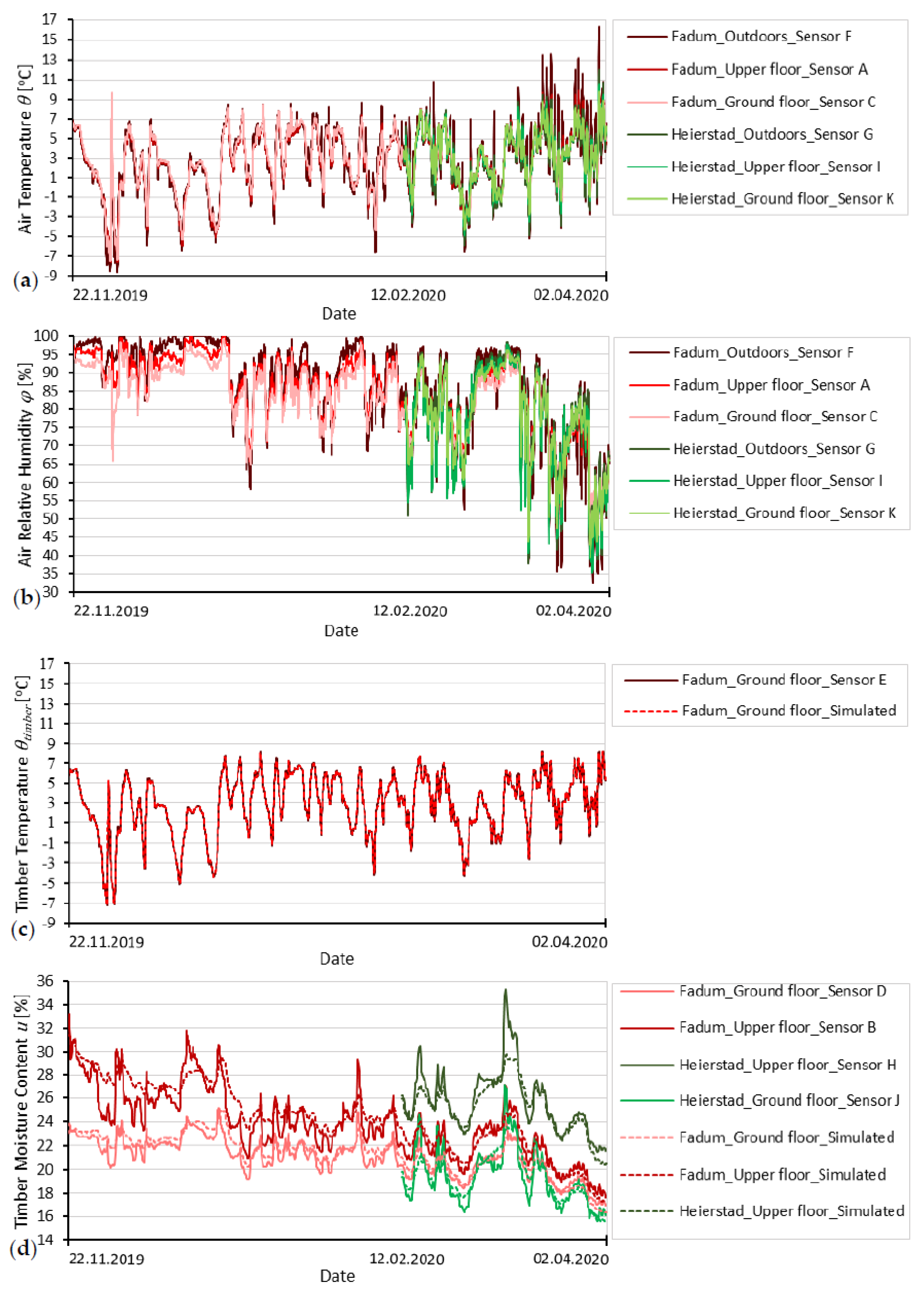
The goodness of fit between measured and simulated test parameters of the hygrothermal performance of selected building components in the two case studies was calculated (Table 5). Five different sets of material properties were examined within the simulations. According to the results (Table 5), the Fadum storehouse and the ground level of the Heierstad loft are most probably made of spruce logs. The upper level of the Heierstad loft, which was reconstructed is 1957, is most probably built of pine logs (Table 5). It is noteworthy that the measurements do not cover the whole range of the hygrothermal performance of the components during a year (Figure 11). In addition, they include incidents within the capillary region where the actual performance of the logs cannot be accurately simulated (Figure 11b,d). Hence, a longer period of measurements, e.g., one year, would provide more robust results. During the summer period, the material temperatures are expected to be significantly higher than the ones presented in Figure 11c, while the moisture content is expected to produce lower values than the ones depicted in Figure 11d. For the certain study site, the periods that the temperature and humidity conditions are favorable for mold growth and, thus, it would be interesting to have measurements for are typically from March to May and from August to October [11].
In regard to the monitored temperatures (Figure 11a,c) and the air relative humidity (Figure 11b), there are no significant differences between the indoors and outdoors environments. This is because the buildings have openings without transparent elements and they do not have HVAC systems. Among the different interior environments, the ground level of the two buildings is the one with the more stable conditions.
The monitored moisture content of the log walls is at very high levels, exceeding the values that are considered critical for mold growth. The low temperatures during the same period are the main reason that the conditions are unfavorable for mold or other wood-destroying microorganisms to grow.
3.3. Past, Present, and Future Climate Conditions
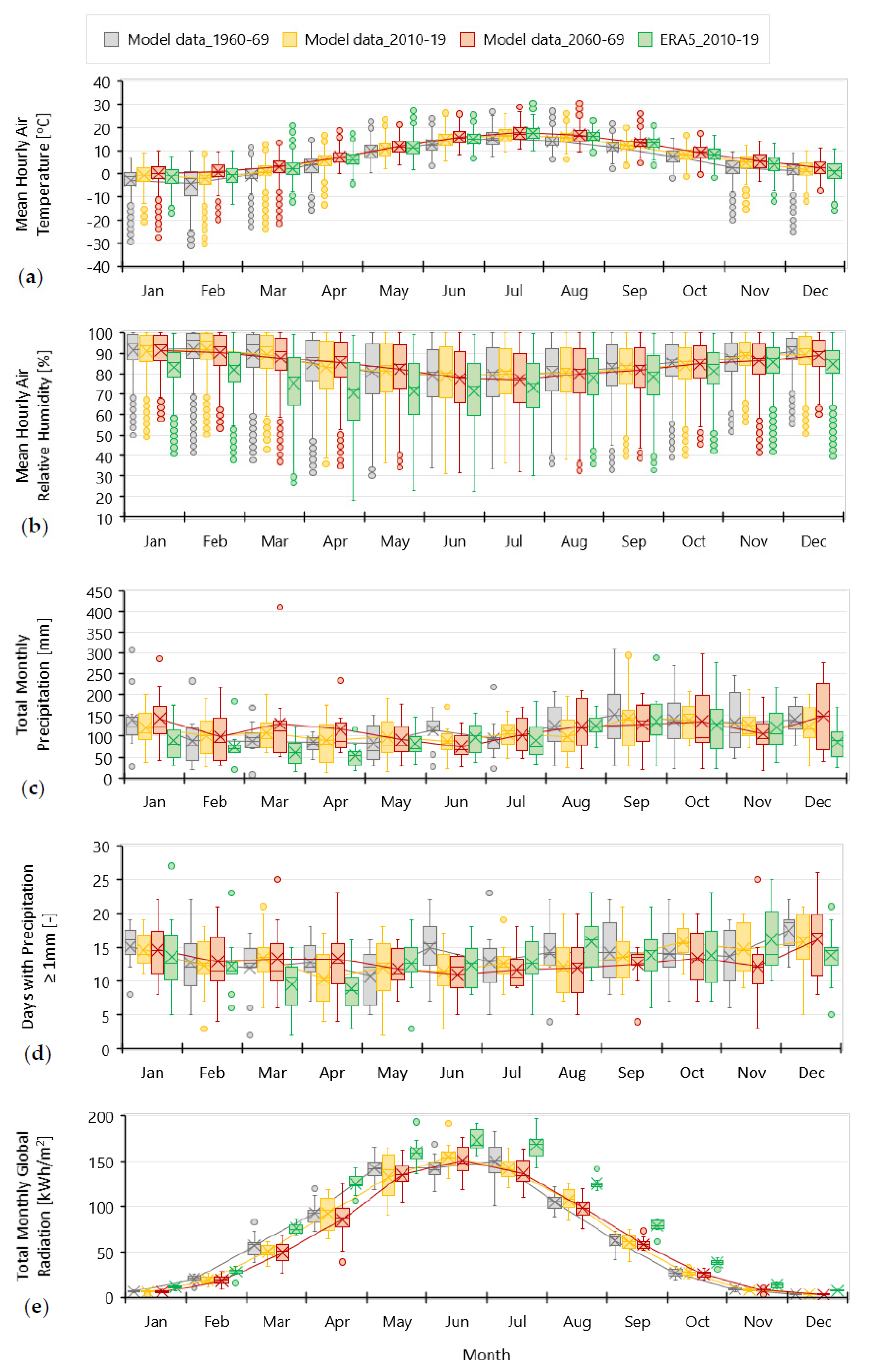
Climate data for three different decades, i.e., 1960–1969 (referred to as past), 2010–2019 (referred to as present), and 2060–2069 (referred to as future), derived from the MPI-ES-LR_REMO2015 model were used for the examination of the climatic changes occurring throughout the years. A fourth climate file with data derived from the ERA5 reanalysis for the period 2010–2019 (current) was used in order to examine the accuracy of the climate model data. The climate parameters that mostly affect the hygrothermal performance of the building components are presented in Figure 12.
The signal of climate change in terms of the air temperature (Figure 12a) is an average increase of 1.6 °C from past to current conditions, and 1.2 °C from current to potential future conditions. The air temperatures are slightly underestimated in the model data, showing an average difference of 0.3 °C compared to the ERA5 reanalysis.
According to the climate model data, the air relative humidity remains at the same levels under past, current, and potential future conditions, with an average value of approximately 85% (Figure 12b). The air relative humidity is overestimated significantly by the climate model data since, according to the ERA5 reanalysis dataset, its average value is 78%.
In some months, the precipitation levels seem to decrease slightly from past to current conditions and to increase from current to future conditions (Figure 12c). However, precipitation levels vary considerably between different years in the region so, based on 10-year periods, it is hard to consistently detect any trends and the results might be different based on a continuous data series. Nevertheless, in winter, from December to April, the highest precipitation level is projected for the latest period 2060–2069. This agrees with most of climate model simulations, indicating increasing wintertime precipitation in Southern Norway, and in Northern Europe in general, while only small changes are usually projected for summer precipitation [45,46]. At the same time, the number of days with precipitation (greater than 1 mm) is projected to change little in winter and spring, and decrease slightly in summer and autumn (Figure 12d). The climate model data overestimate significantly the precipitation. The number of days with precipitation is overestimated by the climate model for the period from December to April, while it is underestimated during the summer period.
The global radiation incident on a horizontal surface shows a slight decrease throughout the years, while it is underestimated according to the climate model data.
3.4. Hygrothermal Performance of Building Elements
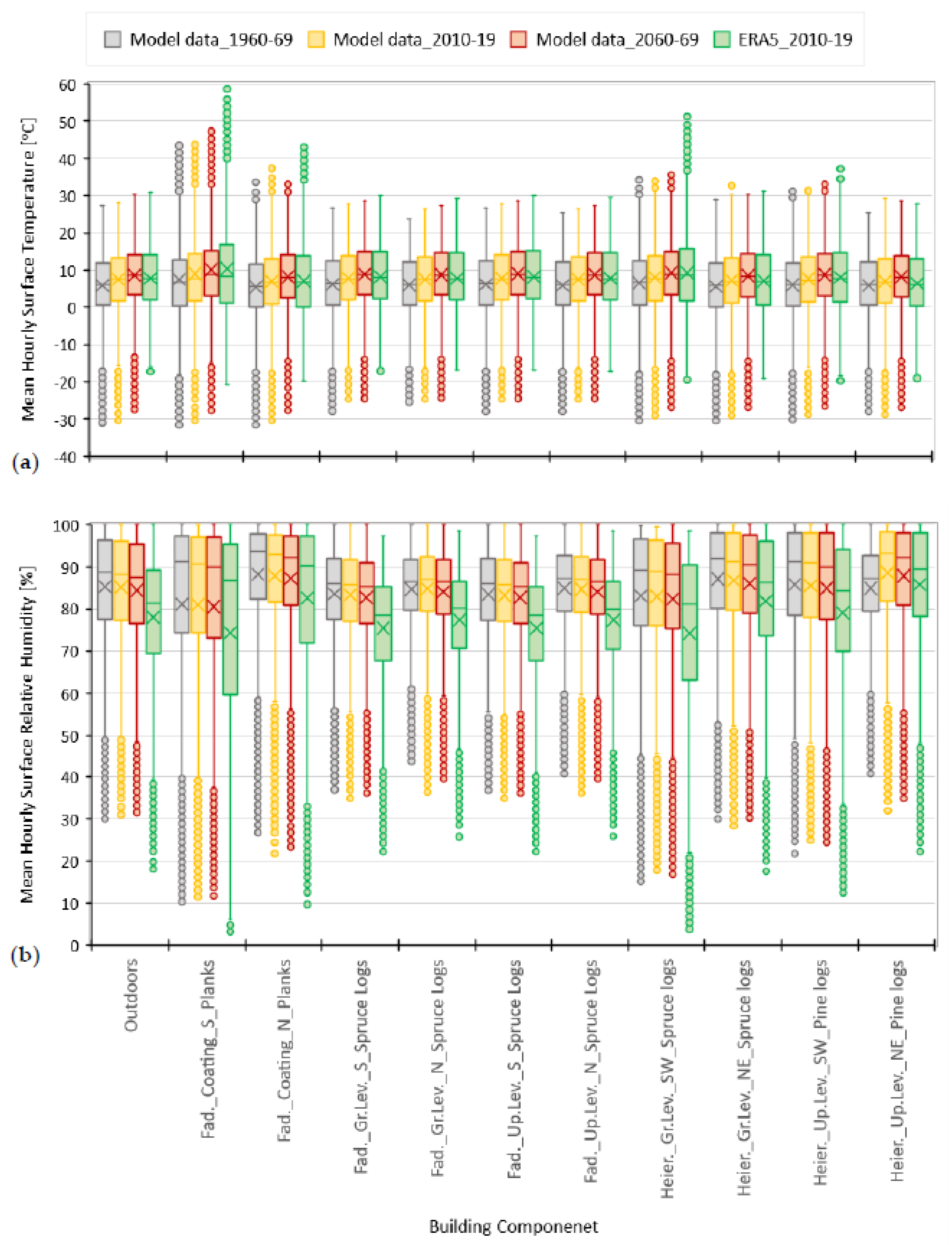
The surface temperature and the surface relative humidity of selected exterior surfaces of the two buildings are presented in Figure 13. Significant differences are observed on the range of the surface temperature and the surface relative humidity according to the exposure environment. The greatest range is observed at the south-oriented surfaces and the smallest one at the surfaces that are protected under the coating/shed of the Fadum storehouse. Moreover, substantive differences are observed among the average values of the surface temperature and the surface relative humidity according to the environment of exposure. The greatest differences are noticed at the coating of the Fadum storehouse. Specifically, pursuant to the data derived from the ERA5 reanalysis, the average value of the surface temperature of the south-oriented side of the coating is 3.18 °C higher than the respective one at the north-oriented side. In addition, according to the data derived from the ERA5 reanalysis, the surface relative humidity at the south-oriented side of the coating is 8% lower than the respective one at the north side. Thus, it is apparent that, for a given period of time, the surface temperature and the surface relative humidity vary significantly based on the orientation.
The surface temperatures simulated with the climate model data were underestimated, while the surface relative humidities were overestimated. Moreover, the differences among different orientations, and especially between south and north, were underestimated significantly based on the data derived from the used climate model. This was mainly due to the underestimation of the incident solar radiation (Figure 12).
The signal of climate change for all surfaces shows an increase of the surface temperature and a slight decrease of the surface relative humidity. The signal of climate change is more intense in the case of north-oriented surfaces and less intense in the case of south-oriented surfaces. The most important changes are observed in the case of the coating of the Fadum storehouse. Specifically, the average value of the surface temperature increases from the past to the future conditions as follows: 2.7 °C at the south and 2.8 °C at the north. Moreover, the average value of the surface relative humidity from the past to future conditions shows a decrease of 0.5% at the south and 1.0% at the north. It is also observed that the differences among all the cardinal orientations become smaller throughout the years.
3.5. Mold Risk
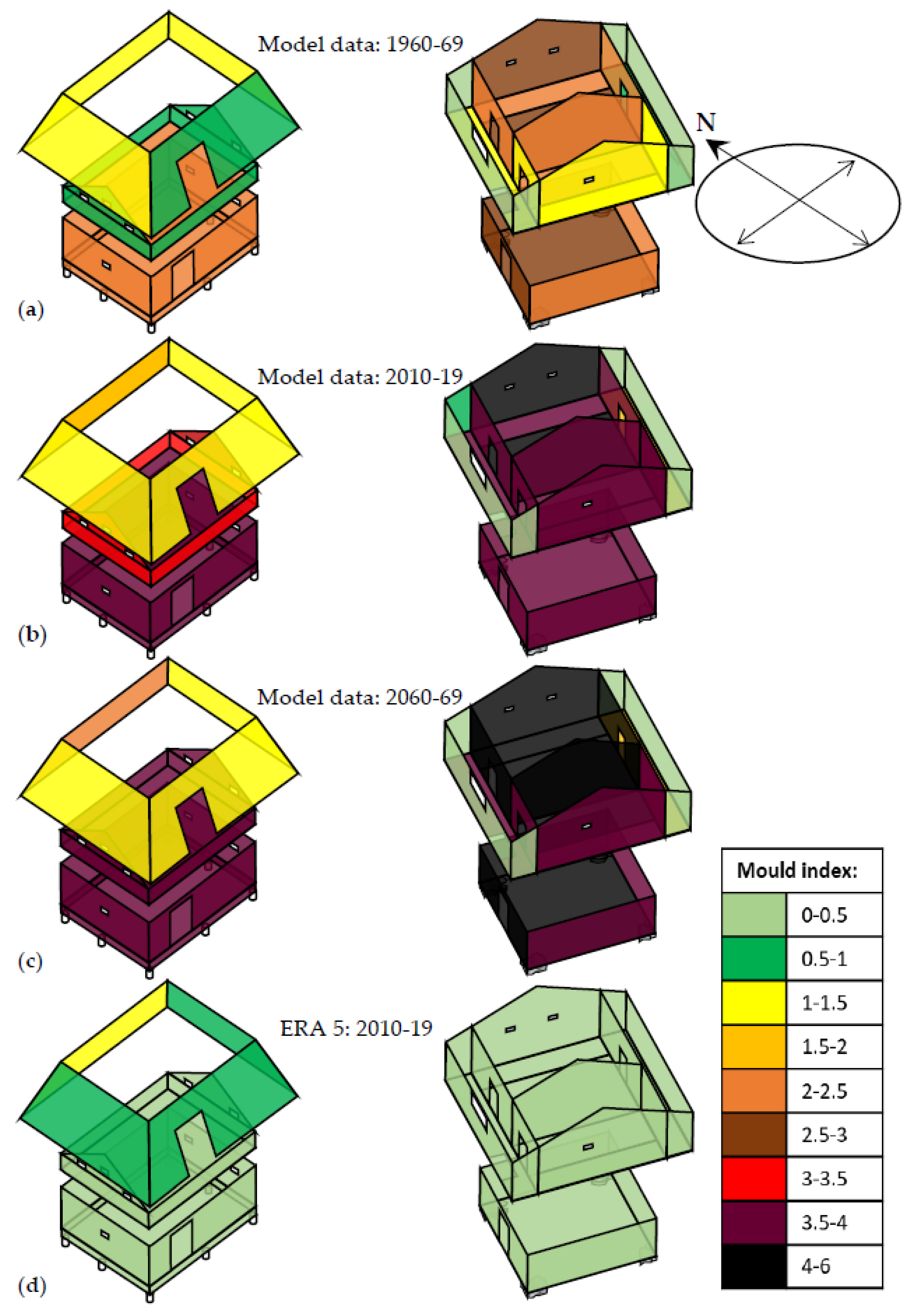
The type of wood (i.e., softwood or hardwood), the type of surface (i.e., planed or rough), the sensitivity of the surface to mold growth (i.e., different sensitivity classes by taking into account that the final surface is sapwood, heartwood, or tar treatment), the surface temperature, and the surface relative humidity were taken into account for the calculation of the mold index of the building components. The four different climate excitations described in the previous chapters were taken into account. The different types of surfaces found at the two case studies, in ascending order regarding their sensitivity to mold growth, are: (i) the exterior surfaces treated with tar, (ii) the surfaces of the planks that have no treatment, (iii) the surfaces of logs that have no treatment, and (iv) the exterior degraded surfaces (due to weathering, checks, and splits). For the assessment of the mold risk of the building components, it is taken into account that mold indices (M) from 0 to 1 are acceptable. That is because the germination process starts at M = 1. Mold indices from 1 to 3 are considered as a risk for the mold growth on the building elements. The mold index M = 3 is the threshold over which mold can be detected by the naked eye and new mold fungi spores are produced. Mold indices above 3 are considered as significant risk and are not acceptable. Considering the aforementioned categorization of the mold index values, in Figure 14, the mold indices from 0 to 1 are depicted with different shades of green, the mold indices from 1 to 3 are depicted with different shades of yellow, and the mold indices from 3 to 6 are depicted with different shades of red.
3.5.1. Current Conditions
First and foremost, the current conditions of the two case studies based on the climate data derived from the ERA5 reanalysis will be discussed. According to the results of the mold growth model, all exterior surfaces treated with tar have no mold risk at all (M = 0). The untreated planks that are exposed to the exterior environment, i.e., the exterior surfaces of the coating of the Fadum storehouse, have a different mold risk depending on their orientation. These differences are depicted in Figure 14d, in which the average values of the annually maximum mold index of the exterior surfaces of the coating are presented. The surface with the highest mold risk is the north-oriented one, with a maximum mold index of 1.3 for the period 2010–19. In contrast, the surface with the lowest mold risk is the south-oriented one, with a maximum mold index of 0.6 during the same period. The untreated planks exposed to the interior environment, i.e., the planks at the roof of the two buildings, and at the walls of the northwest and southeast cantilevers of the Heierstad loft (Figure 14d), are not threatened by mold. In addition, the interior untreated surfaces of the logs are not threatened by mold (Figure 14d). The degraded exterior surfaces (positions with extreme weathering, checks, and splits) that are exposed to rain and solar radiation have significant mold risk. In these cases, the maximum annual mold index fluctuates between 4.5 and 6. This observation underlines the importance of the immediate cleaning and treatment of the damaged surfaces. The degraded exterior surfaces of the floors of the two buildings, which are not exposed to rain and solar radiation, have a maximum mold index of 1.5 during the period 2010–19 and, thus, their risk is not significant. Finally, the degraded exterior surfaces that are protected under the coating of the Fadum storehouse have mold indices lower than 1 and, thus, they are not threatened by mold.
3.5.2. Impact of Climate Change
The mold risk of the surfaces of the two buildings is clearly overestimated by the climate model data. However, the results from the climate model are useful to highlight future changes in sensitivity to mold growth, even though the effect is exaggerated. The exterior surfaces treated with tar are not threatened by mold. Specifically, the maximum mold index occurring on a surface of this category is M = 0.1. The untreated planks that are exposed to the exterior environment have an increase of their mold risk due to climate change. In Figure 14a–c, it can be seen that the increase of the mold index of the exterior surfaces of the coating of the Fadum storehouse depends on their orientation. The increase of the mold index is greater in the case of the north-oriented surface. The mold risk of the untreated planks that are exposed to the interior environment, i.e., the planks at the roof of the two buildings and at the walls of the northwest and southeast cantilevers of the Heierstad loft, do not change due to the climate change (Figure 14a–c). The interior untreated surfaces of the logs of the two buildings have an increase of their mold risk due to climate change. This increase is even more significant from the past to the current conditions. In addition, in both buildings, the interior surfaces of the north-oriented log walls are at a higher mold risk (Figure 14a–c). Finally, all exterior degraded surfaces have significant mold risk under past, current, and future conditions that is intensified due to climate change.
At a given room, very similar mold indices are observed among the interior surfaces of the same surface category (Figure 14). This observation indicates that the air temperature and the air relative humidity of the room can be used instead of the surface temperature and the surface relative humidity as a simplification. At this point, it is worth mentioning that, in Figure 14, the floor of the upper level in both buildings and the log walls of the Heierstad loft that are exposed in both sides to the interior environment are represented by their surface with the highest mold risk. At the Fadum storehouse, the surfaces at the ground level have higher mold risk than the upper level. At the Heierstad loft, higher mold risk occurs at the surfaces of the ground level, secondly at the upper level at the northeast-oriented room, thirdly at the southwest-oriented room, fourthly at the northwest-oriented cantilever, and lastly at the southeast-oriented cantilever. It is worth mentioning that the most aggravated surfaces of the Heierstad loft according to the numerical simulations results (Figure 14) are the same as those where fungal growth was detected in reality (Figure 7). In the case of the Fadum storehouse, both simulations (Figure 14) and reality (Figure 6 and Figure 7) underline that the north-oriented surfaces are more vulnerable to fungal colonization.
3.5.3. Surface vs. Air Temperature and Relative Humidity
The calculation of the surface temperature and the surface relative humidity of the building components, given the outdoor climate from the models, is important for the production of accurate and robust assessment of their mold risk. However, it is a computationally demanding process. In addition, considering that the buildings have openings without transparent elements, are not occupied, and do not have HVAC systems, their indoor and outdoor conditions do not differ significantly. For these reasons, it was examined whether the atmospheric temperature and the relative humidity could be effectively used for the assessment of the mold risk instead of the surface air temperature and the surface air relative humidity. The results (Table 6) show that this simplification is not appropriate for the description of the mold risk at the exterior untreated planks of the coating of the Fadum storehouse (Figure 14). That is because both the mold risk of the surfaces at a given period and the signal of climate change in terms of the mold risk vary significantly based on the orientation. Additionally, this simplification is not appropriate for the interior surfaces of the untreated logs and planks, since it overestimates significantly their mold risk and cannot reproduce the differences occurring among the different rooms (Figure 14 and Table 6).
4. Conclusions
The focus of the current research is on investigating the impact of climate change on the mold risk of two historic timber buildings located in the county of Vestfold, Norway. Climate data from REMO2015 driven by the global model MPI-ESM-LR were used in order to take into account the climate change. The climate data refer to the past, present, and potential future climate conditions. After selecting proper material properties for the building components of the two constructions, and given the outdoors climate, whole-building hygrothermal simulations were employed in order to calculate the temperature and the relative humidity on the surface of the building elements. Given the transient hygrothermal conditions and certain characteristics of the timber surfaces, the updated VTT mold model was used in order to calculate their mold index.
Based on the climate data from the MPI-ES-LR_REMO2015 model, it is concluded that there is an increased mold risk of the two timber constructions due to climate change. This impact of climate change is more severe in the case of the untreated logs exposed, either in the outdoors or the indoors environment. It is also significant in the case of the untreated planks which are exposed to the outdoors environment, e.g., the planks of the coating/shed of the Fadum storehouse. The surfaces which are treated are not threatened by mold risk due to climate change. In addition, the untreated surfaces of the planks which are exposed to the indoors environment are not threatened by mold due to climate change. It was also observed that the increase of the mold risk due to climate change is more intense in the case of the horizontal surfaces, i.e., ceilings and floors, and the north-oriented vertical or inclined surfaces. According to the employed numerical simulations, the ceiling at the ground level of the Heierstad loft and the northeast-oriented wall at the upper level of the same building are the most aggravated ones in terms of the mold risk due to climate change. These same surfaces are the ones on which fungal colonization was detected on site.
The results derived from the MPI-ES-LR_REMO2015 model overestimate significantly the mold risk of the two buildings compared to results derived from ERA5 reanalysis. This is mainly attributed to the fact that the MPI-ES-LR_REMO2015 model overestimates significantly the relative humidity and the precipitation compared to the ERA5 reanalysis.
The importance of using the surface temperature and the surface relative humidity as inputs in the updated VTT mold model, and not the atmospheric temperature and the atmospheric relative humidity, is also underlined. The mold risk of the interior surfaces is significantly lower than the respective one that is calculated based on the temperature and the relative humidity of the outdoor air. In the opposite direction, the mold risk of the north-oriented exterior surfaces is higher than the respective risk that is calculated based on the temperature and the relative humidity of the outdoor air.
According to the onsite inspection and the numerical simulation results based on the ERA5 reanalysis climate data, the two buildings are in good condition. The only surfaces that have significant mold risk are the exterior degraded surfaces—which have lost their tar treatment—that are exposed to rain and solar radiation. At this point, it is highlighted that the exterior surfaces should be treated systematically in order for the vulnerable positions that occur due to weathering, checks, and splits to not be exposed to rain and solar radiation. In case of extensive degradation, the building elements should be replaced. Moreover, there is moderate mold risk of the untreated wood surfaces with north orientation that are exposed to the outdoors environment. This observation highlights that the orientation of the untreated timber surfaces influences their mold risk.
It is also worth mentioning that the mold risk of wooden cultural heritage is considered vital, as it involves health hazards, aesthetic problems, and implications on other wood deteriogens’ niches. It is possible that, in the near future, proper cleaning from mold growth will be needed for the untreated logs in the interior of the historic buildings on a periodic basis.
Author Contributions
Conceptualization, P.C. and D.K.; methodology, P.C., D.K., I.L., and B.H.; software, P.C.; validation, P.C.; formal analysis, P.C.; investigation, P.C. and D.K.; resources, P.C., D.K., and I.L.; data curation, P.C.; writing—original draft preparation, P.C.; writing—review and editing, P.C., D.K., I.L., and B.H.; visualization, P.C.; supervision, D.K.; project administration, P.C. and D.K.; funding acquisition, P.C., D.K., and I.L. All authors have read and agreed to the published version of the manuscript.
Funding
This work is a part of the HYPERION project. HYPERION has received funding from the European Union’s Framework Program for Research and Innovation (Horizon 2020) under grant agreement no. 821054. The content of this publication is the sole responsibility of Oslo Metropolitan University and the Finnish Meteorological Institute and does not necessarily reflect the opinion of the European Union.
Institutional Review Board Statement
Not applicable.
Informed Consent Statement
Not applicable.
Data Availability Statement
Acknowledgments
We would like to thank Jørgen Solstad, consultant at Vestfold county culture department, and the personnel of the Slottsfjell museum for providing information and access to the two historic timber buildings examined in the current research.
Conflicts of Interest
The authors declare no conflict of interest.
References
- Sabbioni, C.; Brimblecombe, P.; Cassar, M. The Atlas of Climate Change Impact on European Cultural Heritage: Scientific Analysis and Management Strategies; Anthem Press: London, UK; New York, NY, USA, 2010. [Google Scholar]
- Fatorić, S.; Seekamp, E. Are cultural heritage and resources threatened by climate change? A systematic literature review. Clim. Chang. 2017, 142, 227–254. [Google Scholar] [CrossRef]
- Leissner, J.; Kilian, R.; Kotova, L.; Jacob, D.; Mikolajewicz, U.; Broström, T.; Ashley-Smith, J.; Schellen, H.L.; Martens, M.; van Schijndel, J. Climate for Culture: Assessing the impact of climate change on the future indoor climate in historic buildings using simulations. Herit. Sci. 2015, 3, 38. [Google Scholar] [CrossRef]
- Brimblecombe, P. Refining climate change threats to heritage. J. Inst. Conserv. 2014, 37, 85–93. [Google Scholar] [CrossRef]
- Howard, A.J.; Knight, D.; Coulthard, T.; Hudson-Edwards, K.; Kossoff, D.; Malone, S. Assessing riverine threats to heritage assets posed by future climate change through a geomorphological approach and predictive modelling in the Derwent Valley Mills WHS, UK. J. Cult. Herit. 2016, 19, 387–394. [Google Scholar] [CrossRef] [Green Version]
- Kaslegard, A.S. Climate Change and Cultural Heritage in the Nordic Countries; Nordic Council of Ministers: Copenhagen, Sweden, 2011. [Google Scholar]
- Kelman, I.; Haugen, A.; Mattsson, J. Preparations for climate change’s influences on cultural heritage. Int. J. Clim. Chang. Strateg. Manag. 2011. [Google Scholar] [CrossRef]
- The Hyperion Project. Available online: https://www.hyperion-project.eu/ (accessed on 25 May 2021).
- Huijbregts, Z.; Schellen, H.; Martens, M.; van Schijndel, J. Object damage risk evaluation in the European project Climate for Culture. Energy Procedia 2015, 78, 1341–1346. [Google Scholar] [CrossRef] [Green Version]
- Huijbregts, Z.; Kramer, R.; Martens, M.; Van Schijndel, A.; Schellen, H. A proposed method to assess the damage risk of future climate change to museum objects in historic buildings. Build. Environ. 2012, 55, 43–56. [Google Scholar] [CrossRef]
- Choidis, P.; Tsikaloudaki, K.; Kraniotis, D. Hygrothermal performance of log walls in a building of 18th century and prediction of climate change impact on biological deterioration. E3S Web Conf. 2020, 172, 15006. [Google Scholar] [CrossRef]
- Rajčić, V.; Skender, A.; Damjanović, D. An innovative methodology of assessing the climate change impact on cultural heritage. Int. J. Archit. Herit. 2018, 12, 21–35. [Google Scholar] [CrossRef]
- Sedlbauer, K. Prediction of Mould Fungus Formation on the Surface of/and Inside Building Components. Ph.D. Thesis, University of Stuttgart, Fraunhofer Institute for Building Physics, Stuttgart, Germany, 2001. [Google Scholar]
- Lepage, R.; Glass, S.V.; Knowles, W.; Mukhopadhyaya, P. Biodeterioration models for building materials: Critical review. J. Archit. Eng. 2019, 25, 04019021. [Google Scholar] [CrossRef]
- Vereecken, E.; Roels, S. Review of mould prediction models and their influence on mould risk evaluation. Build. Environ. 2012, 51, 296–310. [Google Scholar] [CrossRef] [Green Version]
- Gradeci, K.; Labonnote, N.; Köhler, J.; Time, B. Mould models applicable to wood-based materials–a generic framework. Energy Procedia 2017, 132, 177–182. [Google Scholar] [CrossRef]
- Ojanen, T.; Viitanen, H.; Peuhkuri, R.; Lähdesmäki, K.; Vinha, J.; Salminen, K. Mold growth modeling of building structures using sensitivity classes of materials. In Proceedings of the 11th International Conference on Thermal Performance of the Exterior Envelopes of Whole Buildings, Buildings XI, Clearwater, FL, USA, 4–9 December 2010. [Google Scholar]
- Woloszyn, M.; Rode, C. Tools for performance simulation of heat, air and moisture conditions of whole buildings. Build. Simul. 2008, 1, 5–24. [Google Scholar] [CrossRef]
- Lengsfeld, K.; Holm, A. Entwicklung und Validierung einer hygrothermischen Raumklima-Simulationssoftware WUFI®-Plus. Bauphysik 2007, 29, 178–186. [Google Scholar] [CrossRef]
- De Wit, M. Hambase: Heat, Air and Moisture Model for Building and Systems Evaluation; Technische Universiteit Eindhoven: Eindhoven, Germany, 2006. [Google Scholar]
- Antretter, F.; Schöpfer, T.; Kilian, R. An approach to assess future climate change effects on indoor climate of a historic stone church. In Proceedings of the 9th Nordic Symposium on Building Physics, Tampere, Finland, 29 May–2 June 2011. [Google Scholar]
- Leissner, J.; Kilian, R.; Antretter, F.; Holm, A. Modelling climate change impact on cultural heritage the European project climate for culture. In Urban Habitat Constructions Under Catastrophic Events: Proceedings of the COST C26 Action Final Conference; CRC Press: London, UK, 2010; p. 45. [Google Scholar]
- Antretter, F.; Kosmann, S.; Kilian, R.; Holm, A.; Ritter, F.; Wehle, B. Controlled Ventilation of Historic Buildings: Assessment of Impact on the Indoor Environment via Hygrothermal Building Simulation. In Hygrothermal Behavior, Building Pathology and Durabilit; de Freitas, V., Delgado, J., Eds.; Springer: Berlin/Heidelberg, Germany, 2013; Volume 1, pp. 93–111. [Google Scholar] [CrossRef]
- Coelho, G.B.; Silva, H.E.; Henriques, F.M. Calibrated hygrothermal simulation models for historical buildings. Build. Environ. 2018, 142, 439–450. [Google Scholar] [CrossRef]
- Erhardt, D.; Antretter, F. Applicability of regional model climate data for hygrothermal building simulation and climate change impact on the indoor environment of a generic church in Europe. In Proceedings of the 2nd European Workshop on Cultural Heritage Preservation EWCHP-2012, Kjeller, Norway, 23–26 September 2012; pp. 99–105. [Google Scholar]
- Delgado, J.; Ramos, N.M.; Barreira, E.; De Freitas, V.P. A critical review of hygrothermal models used in porous building materials. J. Porous Media 2010, 13. [Google Scholar] [CrossRef]
- Zirkelbach, D.; Schmidt, T.; Kehrer, M.; Künzel, H. Wufi® Pro–Manual; Fraunhofer Institute: Munich, Germany, 2007. [Google Scholar]
- Antretter, F.; Winkler, M.; Fink, M.; Pazold, M.; Radon, J.; Stadler, S. WUFI® Plus 3.1-Manual; Fraunhofer Institute: Munich, Germany, 2017. [Google Scholar]
- WUFI® Mold Index VTT. Available online: http://wufi.de/en/software/wufi-add-ons/ (accessed on 25 May 2021).
- Karagiozis, A.; Künzel, H.; Holm, A. WUFI-ORNL/IBP—A North American hygrothermal model. In Proceedings of the 8th Intrnational Conference on Thermal Performance of the Exterior Envelopes of Whole Buildings, Buildings VIII, Clearwater Beach, FL, USA, 2–7 December 2001; pp. 2–7. [Google Scholar]
- Riahi, K.; Rao, S.; Krey, V.; Cho, C.; Chirkov, V.; Fischer, G.; Kindermann, G.; Nakicenovic, N.; Rafaj, P. RCP 8.5—A scenario of comparatively high greenhouse gas emissions. Clim. Chang. 2011, 109, 33–57. [Google Scholar] [CrossRef] [Green Version]
- Jacob, D.; Podzun, R. Sensitivity studies with the regional climate model REMO. Meteorol. Atmos. Phys. 1997, 63, 119–129. [Google Scholar] [CrossRef]
- Giorgetta, M.A.; Jungclaus, J.; Reick, C.H.; Legutke, S.; Bader, J.; Böttinger, M.; Brovkin, V.; Crueger, T.; Esch, M.; Fieg, K. Climate and carbon cycle changes from 1850 to 2100 in MPI-ESM simulations for the Coupled Model Intercomparison Project phase 5. J. Adv. Modeling Earth Syst. 2013, 5, 572–597. [Google Scholar] [CrossRef]
- Jacob, D.; Petersen, J.; Eggert, B.; Alias, A.; Christensen, O.B.; Bouwer, L.M.; Braun, A.; Colette, A.; Déqué, M.; Georgievski, G. EURO-CORDEX: New high-resolution climate change projections for European impact research. Reg. Environ. Chang. 2014, 14, 563–578. [Google Scholar] [CrossRef]
- Taesler, R.; Andersson, C. A method for solar radiation computations using routine meteorological observations. Energy Build. 1984, 7. [Google Scholar] [CrossRef]
- Handbook, A. Fundamentals. Atlanta, Ga; American Society of Heating, Refrigerating and Air Conditioning Engineers, Inc.: Norcross, GA, USA, 2001. [Google Scholar]
- Nik, V.M. Climate Simulation of an Attic Using Future Weather Data Sets-Statistical Methods for Data Processing and Analysis; Chalmers University of Technology: Göteborg, Sweden, 2010; Available online: https://core.ac.uk/download/pdf/70582877.pdf (accessed on 21 June 2021).
- Hersbach, H.; Bell, B.; Berrisford, P.; Hirahara, S.; Horányi, A.; Muñoz-Sabater, J.; Nicolas, J.; Peubey, C.; Radu, R.; Schepers, D. The ERA5 global reanalysis. Q. J. R. Meteorol. Soc. 2020, 146, 1999–2049. [Google Scholar] [CrossRef]
- Norwegian Climate Service Center: Observations and Weather Statistics. Available online: https://seklima.met.no/observations/ (accessed on 25 May 2021).
- Hukka, A.; Viitanen, H. A mathematical model of mould growth on wooden material. Wood Sci. Technol. 1999, 33, 475–485. [Google Scholar] [CrossRef]
- Viitanen, H.; Ojanen, T. Improved model to predict mold growth in building materials. In Proceedings of the 10th International Conference on Thermal Performance of the Exterior Envelopes of Whole Buildings, Buildings X, Clearwater Beach, FL, USA, 2–7 December 2007. [Google Scholar]
- Schmidt, O.; Grimm, K.; Moreth, U. Molecular identity of species and isolates of the Coniphora cellar fungi. Holzforschung 2002, 56, 563–571. [Google Scholar] [CrossRef]
- Heseltine, E.; Rosen, J. WHO Guidelines for Indoor Air Quality: Dampness and Mould; World Health Organization Regional Office for Europe: Copenhagen, Denmark, 2009. [Google Scholar]
- Baxi, S.N.; Portnoy, J.M.; Larenas-Linnemann, D.; Phipatanakul, W.; Barnes, C.; Baxi, S.; Grimes, C.; Horner, W.E.; Kennedy, K.; Larenas-Linnemann, D. Exposure and health effects of fungi on humans. J. Allergy Clin. Immunol. Pract. 2016, 4, 396–404. [Google Scholar] [CrossRef] [Green Version]
- Lehtonen, I.; Ruosteenoja, K.; Jylhä, K. Projected changes in European extreme precipitation indices on the basis of global and regional climate model ensembles. Int. J. Climatol. 2014, 34, 1208–1222. [Google Scholar] [CrossRef]
- Räisänen, J.; Ylhäisi, J.S. CO 2-induced climate change in northern Europe: CMIP2 versus CMIP3 versus CMIP5. Clim. Dyn. 2015, 45, 1877–1897. [Google Scholar] [CrossRef]
- Copernicus Climate Change Service: ERA5 Hourly Data on Single Levels from 1979 to Present. Available online: https://cds.climate.copernicus.eu/cdsapp#!/dataset/reanalysis-era5-single-levels?tab=form (accessed on 25 May 2021).
- NCI ESGF Node. Available online: https://esgf.nci.org.au/search/esgf-nci/ (accessed on 25 May 2021).
Figure 1.
Photographs of (a) the Fadum storehouse and (b) the Heierstad loft taken from south-west.

Figure 2.
The building components have been grouped in four homogeneous categories, highlighted with different colors, based on the type and age of wood that they are made of. The positions of the installed sensors are also highlighted with green color for the air temperature and humidity sensors (A, C, F, G, I, K), blue color for the moisture content sensors (B, D, H, J), and red color for the sensor monitoring the temperature inside the timber (E).

Figure 3.
Moisture storage functions of the wood species that were tested for the selection of proper material properties for the two case studies. The data derive from the WUFI® database.
Figure 3.
Moisture storage functions of the wood species that were tested for the selection of proper material properties for the two case studies. The data derive from the WUFI® database.

Figure 4.
Comparison between (a) air temperature, (b) air relative humidity and (c) precipitation data derived from the Melsom weather station that is located 5 km from the study site, and from the ERA5 reanalysis. In the boxplots the box shows 50% of the data, with median represented as a horizontal bar and the average value highlighted with the ‘x’ symbol. The whisker extends to two standard deviations of the data and the circles represent the outliers.

Figure 5.
The whole-building simulation models of (a) the Fadum storehouse and (b) the Heierstad loft.
Figure 5.
The whole-building simulation models of (a) the Fadum storehouse and (b) the Heierstad loft.

Figure 6.
At the Fadum storehouse, the growth of biological organisms is more intense on (a) the north façade than on (b) the south façade.
Figure 6.
At the Fadum storehouse, the growth of biological organisms is more intense on (a) the north façade than on (b) the south façade.

Figure 7.
(a) Brown-rot fungi (Coniophora puteana) detected at the positions highlighted with red color at the Fadum storehouse. (b) Scopulariopsis colonies and (c) Myxomycetes detected at the positions highlighted with red color at the Heierstad loft.
Figure 7.
(a) Brown-rot fungi (Coniophora puteana) detected at the positions highlighted with red color at the Fadum storehouse. (b) Scopulariopsis colonies and (c) Myxomycetes detected at the positions highlighted with red color at the Heierstad loft.

Figure 8.
Positions of aerosol sampling and fungi colonies grown after 3 days at 25 °C on malt agar (plates on the left side of the pictures) and on DG-18 agar (plates on the right side of the pictures).
Figure 8.
Positions of aerosol sampling and fungi colonies grown after 3 days at 25 °C on malt agar (plates on the left side of the pictures) and on DG-18 agar (plates on the right side of the pictures).

Figure 9.
Fungal concentration in the two case studies considering the number of colony forming units found on the plates. The maximum acceptable value of 500 CFU/m3 for noncontaminated indoor environments [43] is highlighted with the red line.
Figure 9.
Fungal concentration in the two case studies considering the number of colony forming units found on the plates. The maximum acceptable value of 500 CFU/m3 for noncontaminated indoor environments [43] is highlighted with the red line.

Figure 10.
Fungal structures of (a) Penicillium spp., (b) Aureobasidium spp., (c) Cladosporium spp., (d) Alternaria spp., (e) Mucor spp., and (f) Scopulariopsis spp. after methylene blue staining.
Figure 10.
Fungal structures of (a) Penicillium spp., (b) Aureobasidium spp., (c) Cladosporium spp., (d) Alternaria spp., (e) Mucor spp., and (f) Scopulariopsis spp. after methylene blue staining.

Figure 11.
Measurements of the (a) air temperature and (b) relative humidity, which have been used as boundary conditions in the hygrothermal models, and both measured and simulated (c) temperature and (d) moisture content in the timber building components.
Figure 11.
Measurements of the (a) air temperature and (b) relative humidity, which have been used as boundary conditions in the hygrothermal models, and both measured and simulated (c) temperature and (d) moisture content in the timber building components.

Figure 12.
Comparison among (a) air temperature, (b) air relative humidity, (c,d) precipitation and (e) radiation data derived from the MPI-ESM-LR_REMO2015 model and ERA5 reanalysis. In the boxplots the box shows 50% of the data, with median represented as a horizontal bar and the average value highlighted with the ‘x’ symbol. The whisker extends to two standard deviations of the data and the circles represent the outliers.

Figure 13.
Distribution of (a) hourly surface temperature and (b) hourly surface relative humidity for the exterior surface of selected building components. In the boxplots the box shows 50% of the data, with median represented as a horizontal bar and the average value highlighted with the ‘x’ symbol. The whisker extends to two standard deviations of the data, and the circles represent the outliers.

Figure 14.
Average values of annually maximum mold indices under (a) past, (b) current, and (d) future climate conditions, considering climate data from MPI-ESM-LR_REMO2015 model. (d) Respective results for the current conditions by considering climate data from the ERA5 reanalysis. The results refer to the interior surfaces of the building components, with the exception of the coating of the Fadum storehouse where the exterior side is taken into account.


Table 1.
Inputs, outputs, and origin of the measurements to validate the outputs of the simulated hygrothermal performance of selected building components.
Table 1.
Inputs, outputs, and origin of the measurements to validate the outputs of the simulated hygrothermal performance of selected building components.
| Group | 1D Hygrothermal Simulations | Origin of Measurements to Validate the Output | |||
|---|---|---|---|---|---|
| Component | Input Climate | Output | |||
| Interior θ, φ | Exterior θ, φ | ||||
| II | Log at the southern wall of the ground level of the Fadum storehouse | Sensor C | Sensor F | θtimber 1 | Sensor E |
| u 1 | Sensor D | ||||
| Log at the southern wall of the upper level of the Fadum storehouse | Sensor A | Sensor F | u 1 | Sensor B | |
| III | Log at the northwest wall of the ground level of the Heierstad loft | Sensor K | Sensor G | u 1 | Sensor J |
| IV | Log at the northwest wall of the upper level of the Heierstad loft | Sensor I | Sensor G | u 1 | Sensor H |
1 The simulated outputs of θtimber (temperature inside the timber) and u (moisture content) were calculated as the average values along a depth of 10 mm from the inner surface of the building components.
Table 2.
Description of the mold growth index [41].
Table 2.
Description of the mold growth index [41].
| Index | Growth Rate | Description |
|---|---|---|
| 0 | No growth | Spores not activated |
| 1 | Small amounts of mold on surface (microscope) | Initial stages of growth |
| 2 | <10% coverage of mold on surface (microscope) | - |
| 3 | 10–30% coverage of mold on surface (visual) | New spores produced |
| 4 | 30–70% coverage of mold on surface (visual) | Moderate growth |
| 5 | >70% coverage of mold on surface (visual) | Plenty of growth |
| 6 | Very heavy and tight growth | Coverage around 100% |
Table 3.
Parametrization of the updated VTT mold model based on the features of the examined surfaces.
Table 3.
Parametrization of the updated VTT mold model based on the features of the examined surfaces.
| Surface Description | W | SQ | k1 | k2 (Mmax) | Cmat | ||||
|---|---|---|---|---|---|---|---|---|---|
| M < 1 | M ≥ 1 | A | B | C | φmin [%] | ||||
| Log/plank treated with tar | 0 | 0 | 0.072 | 0.097 | 0.0 | 5 | 1.5 | 85 | 1 |
| Log without treatment | 0 | 0 | 1.000 | 2.000 | 1.0 | 7 | 2.0 | 80 | 1 |
| Plank without treatment | 0 | 0 | 0.578 | 0.386 | 0.3 | 6 | 1.0 | 80 | 1 |
| Degraded surface (positions with cracks, splits, etc.) | 0 | 1 | 1.000 | 2.000 | 1.0 | 7 | 2.0 | 80 | 1 |
Table 4.
Fungi genera identified from the samples collected from the two case studies.
| Fungi Genera | Fadum Storehouse | Heierstad Loft |
|---|---|---|
| Penicillium spp. | ✓ | ✓ |
| Aureobasidium spp. | ✓ | ✓ |
| Cladosporium spp. | ✓ | ✓ |
| Alternaria spp. | ✓ | ✓ |
| Scopulariopsis spp. | ✓ | ✓ |
| Mucor spp. | ✓ |
Table 5.
Selection of material properties for the logs of the two case studies by examining the goodness of fit between measured and simulated hygrothermal performance.
Table 5.
Selection of material properties for the logs of the two case studies by examining the goodness of fit between measured and simulated hygrothermal performance.
| Group | Group Description | Test Component | Test Parameter | Goodness of Fit | ||||
|---|---|---|---|---|---|---|---|---|
| a 1 | b 1 | c 1 | d 1 | e 1 | ||||
| II | Logs forming the walls and floors of the Fadum storehouse | Log at the southern wall of the ground level | θtimber | 92.9 | 92.9 | 93.5 | 94.1 | 90.2 |
| u | 44.5 | 31.1 | 57.4 | 24.5 | 1.74 | |||
| Log at the southern wall of the upper level | u | 56.9 | 17.7 | 57.2 | 38.7 | 4.3 | ||
| III | Logs forming the walls and floors of the ground level of the Heierstad loft | Log at the northwest wall of the ground level | u | 28.3 | 20.7 | 43.0 | 44.2 | 7.7 |
| IV | Logs forming the walls and floors of the upper level of the Heierstad loft | Log at the northwest wall of the upper level | u | 7.2 | 0.3 | 8.29 | 13.2 | 48.3 |
1 The materials are derived from WUFI database and they can be found under the names: (a) Softwood (by Fraunhofer-IBP), (b) Spruce, radial (by Fraunhofer-IBP), (c) Spruce, tangential (by LTH Lund University, Sweden), (d) Scandinavian spruce transverse direction (by NTNU), (e) Pine transverse direction (by NTNU). The color of group of the building components in the first column of the table is in accordance with the color of the material categories in Figure 2. Data in green correspond to the material according to which measurements and simulations have the best fit.
Table 6.
Average values of annually maximum mold indices by taking into account all different substrate surfaces of the case studies, the atmospheric temperature, and the relative humidity under four different climatic excitations.
Table 6.
Average values of annually maximum mold indices by taking into account all different substrate surfaces of the case studies, the atmospheric temperature, and the relative humidity under four different climatic excitations.
| Surface Description | Climate Model Data | ERA5 | ||
|---|---|---|---|---|
| 1960–69 | 2010–19 | 2060–69 | 2010–19 | |
| Log/plank treated with tar | 0.0 | 0.0 | 0.0 | 0.0 |
| Log without treatment | 5.7 | 5.7 | 5.8 | 1.1 |
| Plank without treatment | 1.1 | 1.3 | 1.5 | 0.2 |
| Degraded surface (positions with cracks) | 5.8 | 5.8 | 5.9 | 4.5 |
Data (i) in green mean that there is not mold growth risk, (ii) in different shades of yellow mean that there is mold growth risk and (iii) in red mean that there is significant mold growth risk, which is not acceptable.
Publisher’s Note: MDPI stays neutral with regard to jurisdictional claims in published maps and institutional affiliations. |
© 2021 by the authors. Licensee MDPI, Basel, Switzerland. This article is an open access article distributed under the terms and conditions of the Creative Commons Attribution (CC BY) license (https://creativecommons.org/licenses/by/4.0/).
Share and Cite
MDPI and ACS Style
Choidis, P.; Kraniotis, D.; Lehtonen, I.; Hellum, B. A Modelling Approach for the Assessment of Climate Change Impact on the Fungal Colonization of Historic Timber Structures. Forests 2021, 12, 819. https://doi.org/10.3390/f12070819
AMA Style
Choidis P, Kraniotis D, Lehtonen I, Hellum B. A Modelling Approach for the Assessment of Climate Change Impact on the Fungal Colonization of Historic Timber Structures. Forests. 2021; 12(7):819. https://doi.org/10.3390/f12070819
Chicago/Turabian StyleChoidis, Petros, Dimitrios Kraniotis, Ilari Lehtonen, and Bente Hellum. 2021. "A Modelling Approach for the Assessment of Climate Change Impact on the Fungal Colonization of Historic Timber Structures" Forests 12, no. 7: 819. https://doi.org/10.3390/f12070819
Note that from the first issue of 2016, this journal uses article numbers instead of page numbers. See further details here.