Earthquake Early Warning System for Structural Drift Prediction Using Machine Learning and Linear Regressors

Introduction

Seismic risk is one of the main concerns for public authorities in seismic prone regions. Earthquake Early Warning Systems (EEWSs) are complex infrastructures that can mitigate the seismic risk of citizens and losses by the rapid analysis of seismic waves (Gasparini et al., 2011). Typically, EEWS analyzes seismic data in real-time for automatically detects and predict the earthquake size using the first seconds of P-wave signals. Generally, by these pieces of information, EEWSs attempt predicting the ground motion (e.g., Peak Ground Acceleration, PGA) at specified targets. Hence, EEWSs disseminate alerts to targets where the shaking intensity is expected to overcome a damage threshold.

There are two main families of EEWS: on-site and regional systems (Satriano et al., 2011). The on-site approaches use a single station, or a small seismic network, installed near the target. On the other hand, in regional systems, a seismic network is placed near the seismogenic zone, which normally is placed sufficiently far from the target area to protect. Furthermore, on-site systems use P-waves information to directly predict ground motion through empirical scaling laws, while regional ones exploit primarily P-waves, but also S-waves information, from stations close to the epicenter for estimating the source location and magnitude, which in turn are feeding GMPEs (Ground Motion Prediction Equation) for predicting the ground motion at targets.

A fundamental EEWS parameter is the time available to mitigate the seismic risk at a target before damaging ground motion related to S-waves or surface waves reach it (hereinafter called “lead-time”). Depending on the hypocentral distance between seismic source and target, the lead-time of the EEWS approaches is different: at higher distances, the lead-time is greater for regional systems; at shorter distances, on-site EEWSs are faster and can provide useful alerts when the regional systems fail (Satriano et al., 2011).

In the last 2 decades, several works have proposed the use of P-wave features in on-site EEW framework. Wu and Kanamori (2005) proposed the inverse of the predominant period, τ_c, measured on the first 3s of P-wave waveforms to predict the magnitude. The same authors have also proposed the Peak of Displacement, Pd, on 3s window to predict the Peak Ground Velocity, PGV (Wu and Kanamori, 2008). Brondi et al. (2015) used the Pd and the Integral of squared Velocity, IV² to predict the PGV and the Housner Intensity, I_H. Spallarossa et al. (2019) and Iaccarino et al. (2020) explored the use of Pd and the IV² and for predicting PGV and the Response Spectra of Acceleration, RSA, amplitudes at nine periods, respectively, using a mixed-effect regression approach aiming to account for site-effects.

Besides the ground motion in free field, recently, efforts to predict the structural response in EEWS applications have also been proposed (i.e., applications where the Structural Health Monitoring, SHM, meets the EEWS goal to disseminate real-time alerts). The outputs of these methods can, for instance, trigger automatic isolation systems (Chan et al., 2019; Lin et al., 2020) based on damage level predictions through Engineering Demand Parameters (EDP). For example, Picozzi (2012) proposed to combine P-wave features with the structural building response retrieved by interferometry and a multi-sensors system (Fleming et al., 2009) to predict both the earthquake parameters and the structural response. Kubo et al. (2011) proposed a built-in EEWS for buildings that is able to automatically stop the elevator, start an acoustic alert at each floor, and predict displacement intensity and story drift angle at each floor. In perspective, the use of new advanced technologies, such as Internet of Things and 5G, will significantly facilitate for the easy and huge implementation of such systems (D’Errico et al., 2019).

This work aims to explore the use of P-wave parameters (i.e., Pd, IV² and the integral of squared displacement, ID²) to predict the structural response in on-site EEWS applications. In particular, following Astorga et al. (2020), we considered the drift ratio (Dr.) as a robust and reliable parameter to link in the building response. The parameter Dr. is computed as the relative displacement between two sensors in the building (one placed at the top floor and the other at the bottom floor of the building) divided by the height difference between the sensors.

To this purpose, we investigated the performance of different algorithms to develop robust empirical model between our EEWS parameters and Dr Specifically, we explored both Least Square Regression (LSR) and Machine Learning (ML) techniques. Since Mignan and Broccardo (2019) have demonstrated that complex ML models are often overused, one of our goal is to verify whether MLs, considering their complexity and the difficulties in a suitable training, provide advantages or not with respect to simpler linear models in EEW applications.

We investigated four different machine learning regressors: Random Forest (RF, Breiman, 2001), Gradient Boosting (GB, Friedman, 2001), Support Vector Machine (SVM, Cortes and Vapnik, 1995) and K-Nearest Neighbors (KNN, Altman, 1992). These MLs are used to parameterize models aiming to predicting ${\log }_{10}Dr$ from the three P-wave proxies and three time-windows (i.e., 1, 2, and 3 s). For each regressor, we tune two hyper-parameters by comparing the results of K-fold cross-validation (with K = 5) using the training set (Stone, 1974). Then, the best hyper-parameters set is used to train the ML algorithms with the entire training set (i.e., 80% of the data), and finally, we test their performance with a testing set (i.e., 20% of the data). This procedure allows us to assess in a robust way the regression performance. In parallel, we calibrated models also using linear least square regressors (LSR). To this aim, we used two strategies: we calibrated LSR models for single P-wave features (i.e., three P-wave proxies times three time-window lengths); we used all the features together for calibrating LSR models, mimicking what is done for ML. Therefore, we compare the ML performance with the LSR models.

The calibration and performance analysis are carried out by progressive steps, where the complexity of the dataset is increased at each step. In the first analysis, we focused on the Shiodome Annex (ANX) building, a Japanese Steel-Reinforce-Concrete (SRC) building. With its 20 years-long history of earthquakes recording, ANX represents the perfect starting case study to understand the capabilities of the methods.

In the second step, we considered all the Japanese SRC buildings. The rationale in this choice is that, even if they are of the same typology of ANX, we expect that the combination of the buildings response with different site conditions can contribute to inflate the drift variability.

Finally, in the third step we used the complete Japanese dataset, and we performed a residuals analysis de-aggregating them for building and earthquake characteristics. The aim of this last analysis is to explore the possibility of retrieving correction factors that in future EEW applications can be used for improving the drift predictions.

Finally, we verified the validity of the ergodic assumption for the EEWS calibrated models, a typical problem in seismology when models calibrated for a region are applied to data in other areas. To this aim, we applied the models calibrated using the Japanese dataset to the waveforms recorded in U.S. buildings.

Datasets and Methods

Datasets

We consider 3-components waveforms recorded at Japanese and U.S. buildings (Astorga et al., 2020). The considered buildings belong to three different types of construction (Table 1): steel (ST), reinforced concrete (RC) and steel-reinforced concrete (SRC, only Japanese buildings). All buildings have one sensor at the ground floor and one at the top floor. We measure P-waves EEW parameters (Pd, IV², ID²; hereinafter we refer to them in general way as XP parameters) for different signal lengths (i.e., 1, 2 and 3 s) from the station at the ground level, while Dr. is measured using both sensors.

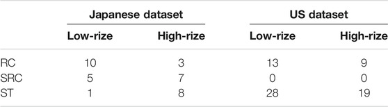
TABLE 1. Dataset summary.

The Japanese dataset (Figure 1A) is made up by 5,942 waveforms collected from 2,930 earthquake recorded at 34 buildings. The magnitude of the events, from the Japan Meteorological Agency (JMA), ranges from M_JMA 2.6 to M_JMA 9, and the epicentral distances vary between 2.2 and 2,514 km.

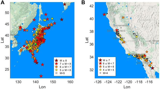
FIGURE 1. Map of the dataset used in the study. The stars indicate the events, the color and the size refer to the magnitude following the legends in the figure. The black squares indicate the buildings, the green one in figure a) is the ANX building.

The US dataset (Figure 1B) is formed by 240 waveforms from 90 events recorded at 69 buildings. The magnitude of these events ranges from Mw 3.5 to Mw 7.3, while the epicentral distance ranges from 2.7 to 391 km.

Table 1 presents the buildings classification according to construction material and height. The largest set of data is available for ANX (Figure 1A), an SRC building in Japan that includes 1,616 waveforms recordings. Since the height is considered important in determining the buildings response, we used the number of floors to divide the dataset into two categories: 1) low-rize buildings when the number of floors is less than eight; 2) high-rize buildings for the others. This classification is similar to the one done in Astorga et al., 2020, but, here, low-rize and mid-rize categories are merged in the low-rize category.

P-Wave Features

Waveforms are filtered using a narrow bandpass Butterworth filter between the frequencies 0.5 and 2 Hz. This choice was made following Astorga et al. (2019) and is motivated by the aim of selecting signals that are strongly related to the structural response. Indeed, for the building as those considered in this study the co-seismic fundamental frequency is usually within this range (Astorga et al., 2020).

Since our objective is to calibrate models for on-site EEW application, we considered as proxy of drift parameters estimated from P-wave signal windows of limited lengths (i.e., 1, 2 and 3 s after the P-waves first arrival). The rationale behind this choice is that the three time windows can allow to capture the temporal evolution of the drift, and also to assess the consistence/robustness of the estimates in time. Furthermore, selecting a fixed time window length in EEW systems is not a trivial task. Indeed, two contrasting effects play a role in taking this decision. From one hand, the signal windows should be as shorter as possible to increase the lead-time. On the other hand, since the rupture duration increases with magnitude, selecting too short time-windows lead to the saturation of the prediction, which results in wrong prediction for large earthquakes (i.e., in analogy with the typical magnitude saturation problem in seismology). In this study, using time windows with maximum length equal to 3 s, we expect our P-wave proxies to saturate around magnitude Mw 7 (e.g., Yamada and Mori, 2009).

To assess the structural response, we consider the dimensionless structural drift, Dr., defined as (Astorga et al., 2020)

where PTD is the Peak of Displacement in the top of the building, PGD is the Peak of Displacement at the ground level of the building and h is the distance between the two sensors.

Concerning the P-waves features, we rely on the peak of displacement (Pd), the integral of the squared velocity (IV²) and the integral of the squared displacement (ID²).

These features are computed on the vertical component following Iaccarino et al. (2020).

where t_p is the first arrival time, t is the window length, d(t) is the displacement, and v(t) is the velocity. Pd is measured in cm, IV² in cm²/s and ID² in cm²∙s. Since we measure these three XPs on three different windows, we have a total of nine different features: ID²_1s, ID²_2s, ID²_3s, IV²_1s, IV²_2s, IV²_3s, Pd_1s, Pd_2s, Pd_3s.

Case Studies

The availability of two rich datasets, relevant to two countries with different building typology and tectonic contexts, motivated us to explore the effect of the dataset complexity in the robustness of EEW model predictions. It is quite common in seismology, and especially in EEW applications, to use an ergodic approach in the use of EEW models. In other words, models calibrated combining datasets from different regions are exported to further areas assuming that regional effects do not play role in the model uncertainty (Stafford, 2014). However, results of recent EEW studies (e.g., among others Spallarossa et al., 2019; Iaccarino et al., 2020) have shown the opposite; that is to say, regional characteristics can play an important role in the robustness and accuracy of the EEW predictions, leading to increase the epistemic uncertainty (Al Atik et al., 2010). For this reason, we proceeded setting four different case studies using datasets of increasing order of heterogeneity. We started calibrating EEW models from a specific building (i.e., ANX in Japan); then, we moved forwards including more buildings from the same typology and region (i.e., SRC from Japan); and then, the same region but with different construction typology. Finally, we applied the models calibrated with Japanese data to those recorded at U.S. buildings. Our strategy of assessing the performance of LSR and ML models in progressively harder conditions (i.e., varying dataset size and composition) aims to unveil eventual drawbacks and limitations in their use.

To set a robust assessment of the models calibrated by different approaches (i.e., ML and linearized algorithms) and datasets (i.e., #1 ANX, #2 SRC-JAPAN, #3 all JAPAN buildings, #4 U.S. buildings), we define a training set (80% of the data) and a testing set (20% of the data) for each of the case studies. In all cases, the data for training and testing are selected by randomly splitting the dataset. The training set is used to tune the model parameters. Then, the trained model is used to predict the drift of the testing set. This will provide a trustworthy way to compare LSR and ML models. This procedure will avoid any bias in the evaluation of the models.

Case 1. The ANX building is considered for a building specific analysis (i.e., the same site conditions and building features characterize all the data). Therefore, the variability of data in terms of amplitude and duration length is, in this case, due to only the within-event and aleatory variability (Al Atik et al., 2010).

Case 2. In the second step of our analysis, we considered the dataset formed by all the data from SRC buildings in Japan. This second dataset is made up by 3,086 waveforms from 2,034 events and 12 buildings (of course including also ANX). This analysis, thus, allows us to study the variability related to different site conditions and building responses.

Case 3. We considered the complete Japanese dataset. With respect to the previous one, this dataset also includes the complexity due to differences in the seismic response between different types of construction.

Case 4. We studied the implications of exporting the retrieved model for Japan to another region. To do this, we apply the models trained on the Japanese dataset to the U.S. dataset. Clearly, this application is expected to be the more difficult since different aspects can play a role in degrading the model prediction capability. First of all, there are well-known tectonic and geological differences between Japan and California. The main difference is that the former is a subduction zone with a prevalence of thrust earthquakes, while, in the latter, most of the earthquakes are associated to strike-slip faults. Another important aspect to account for is that differences may exist within the building type of construction, due to different building design codes between Japan and United States.

Linear Least Square Regression

The selected nine XP_w (see P-Wave Features) are strongly covariant, since they are relevant to the same P-wave signals observed in different domains (i.e., displacement, and velocity) and time (i.e., 1, 2 and 3 s). While ML techniques can address this issue, the LSR approaches are prone to problems in cases where the dependent variables are correlated each other. For this reason, we applied the LSR in two different ways.

In the first approach, we used the features separately. This leads us to have nine different linear models that, for the sake of simplicity, have the same functional form, as:

where XP_w can be any of the P-wave parameters (Eqs 2–4) at a specific window-length w (i.e., 1, 2 or 3 s). We will refer to these models as “LSR XP_w”.

For all these techniques, we calibrated ML models by adopting an approach that mimics increase of information with time typical of EEW applications (i.e., the temporal evolution of time-windows in 1, 2, and 3°s). In particular, for the first time-window (1 s), we use only the 3 P-wave parameters available at that time. For the second time-window (2 s), we consider the information available at this moment (i.e., the features at 1 and 2 s, for a total of 6 features). Finally, for the 3 s window, we use all nine features.

In the second approach we mimic the increasing of information with time typical of EEW applications (i.e., the temporal evolution of time-windows in 1, 2, and 3 s). In particular, for the first time-window (1 s), we use only the 3 P-wave parameters available at that time. For the second time-window (2 s), we consider the information available at this moment (i.e., the features at 1 and 2 s, for a total of 6 features). Finally, for the 3s window, we use all nine features. We will refer to three combined models as “LSR_w”.

In total, we will compare 12 linear models.

Machine Learning Regressors

As previously said, we use four different ML techniques: Random Forest (RF, Breiman, 2001), Gradient Boosting (GB, Friedman, 2001), Support Vector Machine (SVM, Cortes and Vapnik, 1995) and K-Nearest Neighbors (KNN, Altman, 1992). In this section, we shortly present them focusing on hyper-parameters tuned by a K-fold cross validation. Of course, we refer to the referenced works for their deeper understanding.

RF Regressor

RF regressor (Breiman, 2001) is an ensemble of a specified number of decision tree regressors (N_tr). A decision tree regressor works as a flow-chart in which, for each node, a feature is selected randomly to subdivide the data in two further nodes through a threshold. This latter is chosen to minimize the node impurity, as follows:

where N is the number of the training data in the node, y_i is the real value of the target for the ith datum and $\widehat{y}$ is the predicted value of the end node in which the ith point is assigned. The predicted value of the end node is simply the mean value of the data in the end node itself. The depth of the trees is controlled by a tolerance factor that stops the subdivision procedure if the gain in impurity is not enough, or by reaching a maximum depth value M_dep. The final regression is given by the average prediction of all the trees. We select N_tr and M_dep as the hyper-parameters to tune.

GB Regressor

In a similar way to RF, the GB regressor is an ensemble of N_tr decision tree regressors (Friedman, 2001). The main difference between the two is that in GB the steepest descent technique is applied to minimize a least square loss function. In this algorithm, each decision tree plays the role of a new iteration, while the procedure is controlled by the hyper-parameter learning rate (L_r). From preliminary studies, we decide to fix N_tr = 300 and we tune M_dep and L_r.

SVM Regressor

The SVM regressor searches the best hyperplane to predict the target value also minimizing the number of predictions that lies outside an ε-margin from the hyperplane (Cortes and Vapnik, 1995). The result is achieved solving the problem:

where $\omega \in {\mathrm{ℝ}}^p$ and $b\in \mathrm{ℝ}$ are the linear regression parameters for p features, C is a penalty factor, and ${\xi }_i , {\xi }_i^{\ast }$ are positive slack variables representing the distance from the lower or the upper margins. It is worth to note that the slack variables (${\xi }_i \text{and} {\xi }_i^{\ast }$) are both non-zero only if the datum lies inside the margins. Furthermore, to include any nonlinear trends, we used a Gaussian kernel with σ_SVM as variance. In summary, the main hyper-parameters for this technique are ε, C and σ_SVM. Looking at preliminary testing results, we fixed ε = 0.1 and we tuned C and σ_SVM.

KNN Regressor

Finally, the KNN regressor predicts the target of a certain datum as the weighted average of the K_N nearest data target, where the weights are the opposite of the distance (Altman, 1992). This technique is a lazy learner because the training step consists only in the memorization of a training set. We use the Minkowski distance of order p (van de Geer, 1995). We use K_N and p as hyper-parameters to tune.

For all these techniques, we calibrated ML models by adopting an approach similar to the one adopted for combined LSR models. That is to say, we will use all the available features at each second (i.e., 3 features at 1s, 6 at 2s and, finally, nine features at 3s) to calibrate the ML models. In this way, we have three configurations for each ML regressor with a total of 12 ML models. Hereinafter, we will refer to these models as ML_w, where ML can be RF, GB, SVM or KNN, and w is the time window used.

Validation Process

For all ML methods, we apply the logarithm base 10 to all the features and then we standardize them to have a unit variance. For each ML algorithm, we apply a K-fold cross-validation (Stone, 1974) on the training set with K = 5 for each set of hyper-parameters. We use the coefficient of determination R² as comparative score, so as to find the optimal configuration for each model. This effort is done to avoid two critical issues that are well-known with ML techniques: underfitting and overfitting (Dietterich, 1995; Hawkins, 2004; Raschka and Mirjalili, 2017). A model is underfitted when it is too simple and is not able to retrieve good predictions even on the training set (e.g., this can happen also when LSR is performed on strongly non-linear databases). On the other hand, a model is overfitted when it performs very well on the training set but presents a lack of accuracy on the testing set. This problem arises when a model is so complex that it results too linked with the training data variability.

ANX and SRC Analysis

In this section, we analyze the EEW models calibrated considering the ANX and SRC buildings subsets.

Least Square Regression Models

As said above, we develop 12 linear models (i.e., derived combining three P-wave proxies and three different windows, and the combined LSR models) for the two datasets. As example, we show in Figure 2 the results of the regression performed for Pd considering the three windows on the ANX (similar figures are shown for IV² and ID² as supplementary information, Supplementary Figures S1, S2). Figure 2 shows that both the training set (gray circles) and testing set (green triangles) have the same variability around the fit. We report the results of all the linear regressions, for ANX in Table 2, and for SRC in Table 3, whereas the first two columns report the regression parameters as in Eq. 5 (for LSR_w models, we reported the regression coefficients in Supplementary Table S1). Moreover, the third column, σ_train, contains the standard deviation of the residuals for the training set, while the fourth column, σ_test, contains the same but for the testing set. Finally, in the last two columns, we report the R² value for training and testing sets.

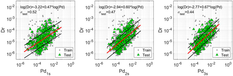
FIGURE 2. Dr. vs. Pd (cm) of the ANX dataset for three different windows. Gray dots refer to train set data. Green dots refer to test set data. The red lines are the least square regression performed for the train set. The black lines, instead, represent the ±σtrain confidence level. The equation of this line is written in the upper part of each figure with its own test residual variability, σ_test.

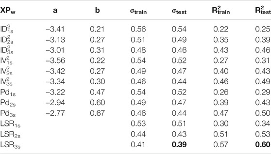
TABLE 2. Least square regression results, ANX dataset.

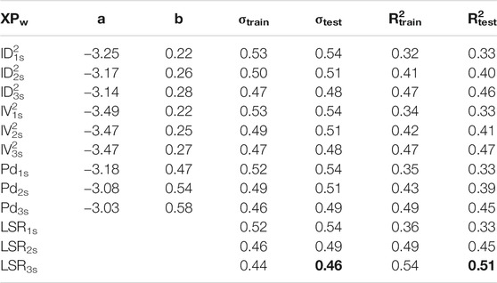
TABLE 3. Least square regression results, SRC dataset.

Looking at the results shown in Table 2 (i.e., ANX), the models perform slightly better on the testing set both in terms of σ and R². This difference is probably due to the different amount of data within the two sets. It is worth to note that the prediction improves with the increasing of the window length for all the models, i.e., looking at Pd, σ_test is 0.52 at 1 s, 0.47 at 2 s and 0.44 at 3 s. In the end, comparing XPs, we note that IV² and Pd have similar performances, while ID² is the worst. The combined models perform always better than the single-feature models looking window-by-window. LSR_3s provides the best performances with σ_test = 0.39 and R²_test = 0.60 (these values are bolded in Table 2).

From Table 3, we can note that the performance of the LSR models for the Japanese SRC buildings is always slightly worse than that for ANX. This result is probably due to the increase in the between-buildings variability of the observations, that can also be affected by different site conditions (we will focus on this important aspect in the following section). An improvement of predictions with the time window lengths is again observed. In this case, the combined models improve the predictions only for 2 s, and 3 s windows. Finally, we obtain again the best results for LSR_3s with σ_test = 0.46 and R²_test = 0.51 (bolded in Table 3).

We show, in Figure 3, the predicted Dr. vs. the real Dr. using the LSR model calibrated using the combined model LSR_w for the three windows on the ANX (Figures 3A–C) and SRC (Figures 3D–F) testing datasets as red triangles. We also plot the standard deviation references as red dashed lines. From these results, we can see the improving of the performances due to the increasing of the window length.

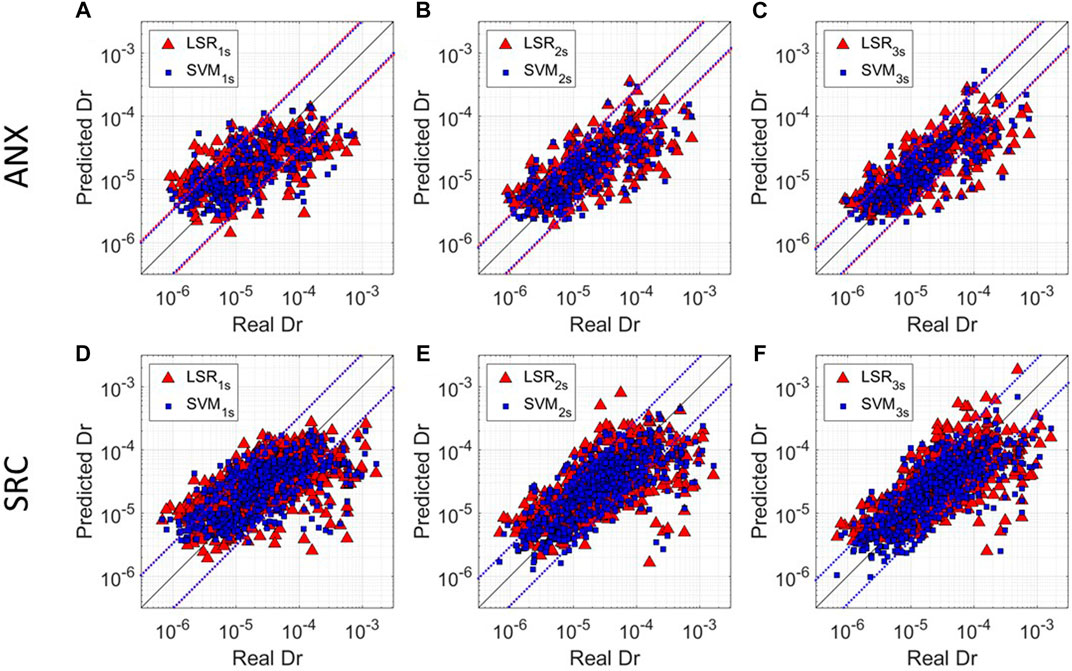
FIGURE 3. Predicted Dr. vs. Real Dr. for three different windows for ANX dataset (A–C) and for SRC dataset (D–F). Red triangles refer to the prediction made least square regression using combined LSR for both datasets measured at the reference window. Blue squares refer to the predictions of the SVM regressor at the reference window. The black line Real Dr. = Predicted Dr. reference line. The dotted lines represent ±σ_train confidence level for LSR (red) and ML (blue) models.

Machine Learning Regression

Tables 4, 5 report the results for 12 ML regression models (see Linear Least Square Regression) for the ANX and SRC datasets, respectively. In these tables, each row refers to a different ML_w. The parameters σ_train and R²_train are the mean of the same parameters obtained by the K-fold cross-validation on the training set. After the training, we apply the calibrated models to the testing dataset.

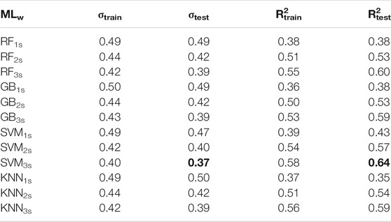
TABLE 4. ML regression results, ANX dataset.

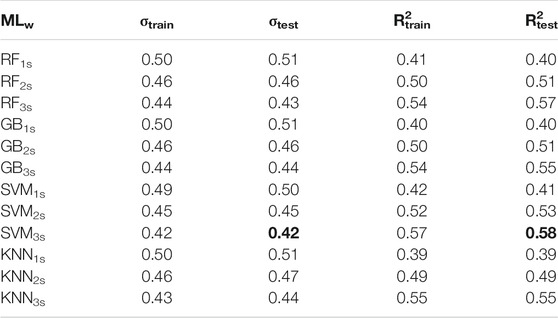
TABLE 5. ML regression results, SRC dataset.

Looking at Table 4, σ_test and R²_test are in general equal or slightly better than the values for the training set. A similar result has been observed also in the least square regression analysis (Table 2). Since our predictions do not worsen on the testing set, we are confident that we are avoiding overfitting. Furthermore, applying ML analyses, the prediction performance is improved by using the longest time window available. Lastly, SVM_3s is the best ML among the tested ones, with σ_test = 0.37 and R²_test = 0.64 (bolded in Table 4).

As for the least square regression analysis results, also in this case we observe that drift prediction worsens increasing the building numbers (i.e., going from ANX to SRC buildings). This result shows us that despite buildings are of the same construction typology, the varying site conditions can play a significant role in increasing the drift estimates variability. As for the ANX analysis, the SVM technique provides the best Dr. predictions; in particular, SVM_3s provides the best model with σ_test = 0.42 and R²_test = 0.58.

Figure 3 shows the comparison between the best LSR model (i.e., combined LSR for both datasets, red triangles) and the best ML technique (i.e., SVM for both datasets, blue squares). As expected, we observe for both datasets that the model prediction improves with the time window length (i.e., predictions and observations get closer to the 1:1 reference line; black line), especially for higher Dr. values.

Our results highlight also that the SVM technique provides slightly better predictions than LSR models for both ANX and SRC datasets. Indeed, the variability of prediction for SVM is smaller than that from the linear regression models. This effect is even more evident looking at low and high Dr. values (Figure 3), for which the linear regression models lead to higher variability in the prediction (i.e., especially for SRC buildings, panels d–f).

Such underestimation increases with drift amplitude, which is clearly function also of the events magnitude. For this reason, we hypothesize that the drift underestimation is due to two main effects: 1, for larger magnitude earthquakes (i.e., Mw > 7.5) the moment rate function is longer than 3 s, leading the maximum time-window (3s) to saturate, which in turns makes it difficult to predict Dr.; 2, differently from most of the datasets, the waveforms of large magnitude events are recorded at very large hypocentral distances and can be dominated by high amplitude surface waves. The dominance of surface waves in such signals can pose a problem to our analyses, because our dataset is mostly dominated by moderate to large magnitude events (the 90% of the Japanese data is between Mw 3.6 and 7.0) and the larger ground motion is related to the S-waves. Therefore, models calibrated for estimating the drift associated to S-waves are not efficient in predicting Dr. associated to very large magnitude earthquakes at large hypocentral distances generating high amplitude surface waves.

The analysis on the ANX and SRC datasets suggest us that it is possible to predict in real-time Dr. using P-wave parameters. The best predictions are obtained using the 3stime-windows and using ML models (i.e., the model SVM_3s).

Japanese Dataset Analysis

In this section, we discuss the development and testing of prediction models considering the entire Japanese dataset.

Least Square Regression Laws

Table 6 reports the results for LSR models calibrated on the Japanese dataset. In this case, we observe that the performances on training and testing set are very similar. Again, we notice an overall worsening of both the scores with respect to the ANX (Table 2) and SRC buildings (Table 3). Clearly, this outcome was expected, given that the Japanese dataset includes more variability than the other two datasets.

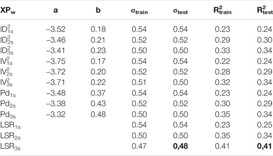
TABLE 6. Least square regression results, Japanese dataset.

In this case, all the P-wave proxies (XPs) show basically the same results in terms of σ_test and R²_test for the same windows. On the other hand, combined LSR models perform slightly better at 2 and 3s. We have the best results for LSR_3s, as in the other cases, σ_test = 0.48 and R²_test = 0.41. Despite such low fitting score can generate skepticism about these LSR models utility, in the following Residual Analysis, we will show that by a residual analysis we can identify some of the component generating the large variability of predictions.

Machine Learning Regression

Table 7 is the analogue of Tables 4, 5 for the Japanese dataset. As for the previous cases, MLs perform better than LSR for the same time window. In this case also, the best model is SVM_3s, with σ_test = 0.45 and R²_test = 0.47. In Figure 4, we compare the predictions of LSR_3s for one of the best LSR models (Table 5) with that of SVM_3s. This comparison clearly shows us that the cloud of SVM_3s estimates is thinner than that for LSR. Despite that, both models seem to saturate above Dr. equal to 4*10^–4.

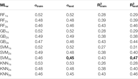
TABLE 7. ML regression results, Japanese dataset.

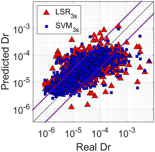
FIGURE 4. Predicted Dr. vs. Real Dr. of the test set for the Japanese dataset for 3s windows. Red triangles refer to the predictions with LSR_3s. Blue squares refer to the predictions of the SVM_3s model. The black line Real Dr. = Predicted Dr. reference line. The dotted lines represent ±σtrain confidence level for LSR (red) and ML (blue) models.

The performances of the calibrated models seem to be worse than those proposed by on-site EEW studies (among others, (Olivieri et al., 2008; Wu and Kanamori, 2008; Zollo et al., 2010; Brondi et al., 2015; Caruso et al., 2017). A direct comparison among different approaches is however unfair. Indeed, despite the appearance, we must consider that generally on-site EEW studies focus on the prediction of ground motion parameters (e.g., peak ground acceleration, PGA) using data collected in free field. On the contrary, in this study, we predict an engineering demand parameter (Dr.) using data from in-building sensors. Our approach is certainly challenging because building responses inflate the variability of our predictions. Furthermore, we must also consider that recent studies (Astorga et al., 2020; Ghimire et al., 2021) explored the prediction of drift from PGA measures using the same dataset considered here and found a prediction variability similar to that of our models. Moreover, other studies, such as Tubaldi et al., 2021, pointed out that event-to-event variability contributes significatively to the uncertainties in the damage prediction, even for single structure models.

Residual Analysis

As we saw in Tables 6, 7, the fitting scores for all the methods are generally rather low. This can be due to numerous factors. One reason can be the lack of information of the EEW input features that, as said, are extracted from p waves, while the final building drift is related to S and surface waves. Anyway, this effect is unavoidable in onsite EEW and also difficult to quantify. Instead, we can try to assess which other factors influence the variability of our methods. So, to better understand the strengths and weaknesses of the calibrated models, we performed a residual analysis (Al Atik et al., 2010). To this purpose, we disaggregate the residuals (predicted minus real Dr. values) by site and event characteristics. In Figure 5, we compare the testing set residuals for the LSR model considering Pd_3s (red error-bars) and the equivalent for SVM_3s (blue error-bars). For each group, we show the mean and the standard deviation of residuals. In all sub-plots of Figure 5, we also show the ±σ_train references for both methods (i.e., 0.50 for Pd_3s represented as red lines, and 0.46 for SVM_3s represented as blue lines).

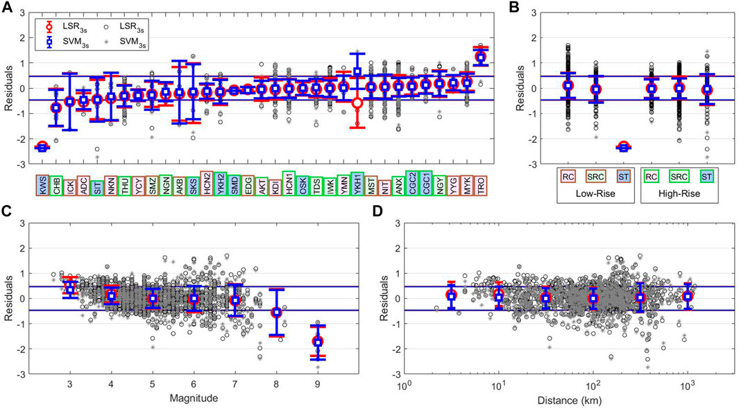
FIGURE 5. Decomposition of the residuals of Dr. prediction for Japanese test set. The residuals are computed as real Dr. - predicted Dr., so positive values mean overestimation, and negative residuals mean underestimation. In each panel we show the residuals for two different models: LSR_3s with circles representing the single prediction and red errorbars representing the mean prediction of the group; SVM_3s with stars for the single prediction and blue errorbars for the group mean. Red and blue lines represent the ±σtrain for LSR_3s and SVM_3s, respectively. The labels in panels (A) and (B) are colored by construction type and height: pink for RC; light green for SRC; blue for ST; brown edges for low-rize; green edges for high-rize. In panel (A) we decompose the residuals by buildings. In (B) we group them by building type of construction and height. In panel (C) we use the magnitude to decompose residuals, the groups are evenly spaced and the errorbars are placed in the center of the bin. In panel (D) the residuals are grouped by distance in km, the groups are evenly spaced and the errorbars are placed in the center of the bin.

Figure 5A presents the residuals grouped by buildings, which are ordered by the mean of the residuals for the two methods. We colored the labels of the buildings by type of construction (pink for RC, light green for SRC, blue for ST) and the edge of the label by the height (brown for low-rize, green for high-rise). At first glance, we observe that the two methods show similar performance in terms of mean of the residuals for all the buildings. Looking at residual variability, however, we observe that in most of the cases ML performs better than LSR, especially for two buildings “YKH1” and “SKS”.

A more detailed examination to residuals variation for different buildings suggests conclusions similar to those of Al Atik et al. (2010) for ground motion prediction equations (GMPEs). These authors, indeed, explored the epistemic uncertainty by splitting it into source, path, and site contributions. If we consider one or many of these factors in our model, we are relaxing the ergodic assumption which states that the variability of the dataset is completely aleatory. The variability of the residuals in Figure 5A is the result of the site-effect, which in our particular case is a term used to describe the response of the soil-structure system that can lead to a very complex behavior. Nevertheless, the full investigation and explanation of the causes of these site conditions is beyond the aim of this paper. In our opinion, the significant variation in residuals shown in Figure 5A is not surprising, being in agreement with other studies (Spallarossa et al., 2019; Iaccarino et al., 2020); which have recently discussed how to reduce the prediction variability considering site-effect terms in EEW model using the mixed-effect regression approach (Pinheiro and Bates, 2000).

As second step, we analyze the residuals grouping them for building characteristics and height (see Table 1 and Figure 5B). Our results show that the mean of residuals for all building groups are close to zero, except for low-rize ST buildings. This latter class, however, includes only the building KWS, that also in the previous analysis showed a peculiar response (Figure 5A). Being the average of residuals consistent with zero, the predictions seem independent from the type of construction and the height of the buildings.

In Figures 5C,D, we show the residuals vs. the event parameters magnitude and distance. It is worth noting that these are not “sufficiency analysis” as intended by Luco (2002). Indeed, in the sufficiency analysis a cinematic parameter is defined as sufficient for predicting an engineering demand parameter (e.g., Dr.) if the predictions are independent from magnitude and distance. To confirm this property, a probabilistic analysis would be needed (Ghimire et al., 2021), but that is beyond the aim of this study.

Figure 5C shows the error bars, the residual mean and standard deviation in bins of 1 unit centered on the magnitude value. From these results, we can clearly see that the magnitude has a great effect on the prediction. In particular, we see that the predictions are good between magnitude 4 and 7, while we overestimate Dr. at lower magnitudes and underestimate Dr. at higher magnitudes. The overestimation at magnitudes lower than 3.5 is probably due to the fact that the predominant frequencies of such events are too high to stimulate an effective response of the building (i.e., we consider a frequencies range between 0.5 and 2 Hz). On the other hand, as previously discussed, the underestimation for magnitude greater than 7.5 is likely due to: 1) the window length of 3 s, which is too small compared to the rupture duration and lead to saturation problems of the prediction; 2) the measured Dr. can be affected by the presence of surface waves associated to large magnitude events. Measures of Dr. form signals dominated by surface waves, indeed, might add non-linear terms to the equation between our XP and Dr. itself. The underestimation at high magnitudes can be also caused by the lower number of recordings in the dataset with respect to those for the smaller magnitudes, i.e. a typical problem for all the EEWS (Hoshiba et al., 2011; Chung et al., 2020). Moreover, another possible bias that big events can introduce are the non-linear responses of site and buildings, especially during long sequence of earthquakes (Guéguen et al., 2016; Astorga et al., 2018). The saturation of Dr. predictions for earthquakes with M > 7.5 is certainly a big issue for the application of the calibrated models in operational EEW systems in areas where very large earthquakes are expected, and further studies are necessary to deal with it. Nevertheless, our results indicate that the calibrated models can be useful in countries characterized by moderate to large seismic hazard (e.g., Italy, Greece, Turkey; where the seismic risk is high due to high vulnerability and exposure). A more in-depth analysis of the performances for EEW systems using the models calibrated is beyond the aim of this study, because it would require target dependent economic cost-benefit analyses (Strauss and Allen, 2016; Minson et al., 2019).

Interestingly, SVM_3s seems providing better results than LSR for both for lowest and highest magnitude events. In our opinion, this result suggests a higher performance of non-linear models.

Finally, Figure 5D shows the residuals grouped by the distance, using 6 bins evenly spaced in logarithmic scale from 10^0.5 to 10³ km. The mean of residuals and the associated standard deviation are plotted at the center of each corresponding bin. We observe that all the residuals are close to zero. Nevertheless, we observe a small overestimation of the prediction at distances lower than 20 km. This effect is partially connected to the overestimation seen for low magnitudes (Figure 5C), because in this range of distances the magnitude is limited between 2.6 and 5.2. In this case too, the machine learning seems able to learn how to solve the bias.

The results of the residual analysis suggest: 1) SVM_3s is confirmed as the best model; 2) decomposing the residuals with respect to buildings, construction type, magnitude, and distance, we found a broad variation of the mean residuals with the buildings typology. This result suggests that site-correction terms should be included in future EEW application to buildings. 3) The residuals are correlated to the magnitude, while they seem be much less dependent from the distance.

US Dataset Application

In the last part of this work, we apply the models calibrated using the Japanese dataset to the U.S. dataset. Our aim is to verify if the usual ergodic assumption often used in EEW application is valid or not, and eventually to look for strategies that could allow to successfully export the models from one region to another.

Least Square Regression Laws

Table 8 reports the results for the linear regression performed on the complete dataset. The most noticeable aspect here is the R²_test column that presents all negative value. This is due to a quite important bias in the prediction of Dr. for U.S. building. In Figure 6, we show the mean residual for U.S. dataset, which are plotted as orange error bars with the length equal to σ_test/σ_train. Since the residuals are computed as differences between predicted and observed Dr., the linear regression of the Japanese dataset underestimates the Dr. of the U.S. buildings of about 1σ. We find a similar bias also for ML techniques. These observations confirm that exporting EEW models among different regions, independently from the algorithm used for their calibration, is not a straightforward operation.

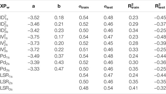
TABLE 8. Least square regression results, complete dataset.

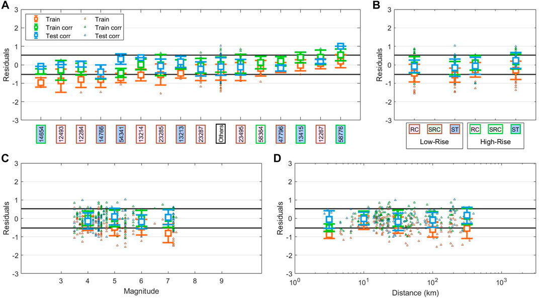
FIGURE 6. Decomposition of the residuals of Dr. prediction for US dataset using Japanese model. The residuals are computed as real Dr. - predicted Dr., so positive values mean overestimation, and negative residuals mean underestimation. In each panel we show the residuals for LSR IV²_2s model in three cases: for the training set without corrections, with orange tringles representing the single prediction and orange errorbars representing the mean prediction of the group; for the training set with magnitude dependent correction with green triangles for the single prediction and green errorbars for the group mean; for the testing set with magnitude dependent correction with light blue triangles for the single prediction and light blue errorbars for the group mean. Black lines represent the ±σ_train for LSR IV²_2s. The labels in panels (A) and (B) are colored by construction type and height: pink for RC; light green for SRC; blue for ST; brown edges for low-rize; green edges for high-rize. The “Others” label is white. In panel (A) we decompose the residuals by buildings. In (B) we group them by building type of construction and height. In panel (C) we use the magnitude to decompose residuals, the groups are evenly spaced and the errorbars are placed in the center of the bin. In panel (D) the residuals are grouped by distance in km, the groups are evenly spaced and the errorbars are placed in the center of the bin.

In the next section, we analyze the causes of this bias, and we propose a solution.

Bias Analysis

We present here the results of the residual analysis carried out on the U.S. buildings predictions. Figure 6 shows the results as orange error-bars for LSR with IV²_2s. We selected this particular model because, as we will show also later, after the application of a correction term it becomes the best predictive model for drift on U.S. buildings.

To correctly evaluate the effectiveness of the method, we divided the U.S. dataset in two subsets (60 and 40%): whereas the first subset is used to compute the correction terms and the second one is used to test the models. The residuals for the corrected model are plotted as green error-bars for the U.S. train set and as light blue for the U.S. test set. We report as reference level the ±σ_train as black lines (see also Table 8).

First, we consider only the uncorrected residuals (i.e., orange error-bars). In Figure 6A, we plot only the results for U.S. buildings with at least 3 records, grouping the remaining ones as “Others”. The buildings are ordered for increasing mean value of residuals. We observe a general smaller variability of the residuals with the buildings than for Japanese buildings (Figure 5A), but at the same time we notice that the majority of the buildings have predictions underestimated and non-zero residuals. These results indicate that there is a bias in the global trend of predictions with respect to the buildings.

Looking at Figure 6B, we can note that, while a small bias is still present for high-rize buildings, the majority of the bias is due to low-rize buildings. However, this difference between building classes is not significant since all the bars are consistent with each other.

In Figure 6C, as for Figure 5C, we notice a strong correlation between residuals and magnitude. We can see, indeed, that the predictions worsen with the increasing of the magnitude.

Finally, in Figure 6D, the residuals for U.S. dataset seem to be not significantly affected by the distance. Indeed, the residuals remain equally underestimated but in the second range that goes from about 6 to 18 km. The anomaly in this range of distances is probably connected to data distribution. In fact, here we find events with magnitude between 3.5–4.5 and we can relate this result with what we observe for low magnitude in Figure 6C.

Bias Correction

In this section, we propose a methodology to account for the bias observed from the residual analysis applied to U.S. buildings drift predictions. To this aim, we borrowed the strategy adopted in seismic hazard studies where the decomposition of the variability in the ground motion predictions can be used to improve the estimates (Al Atik et al., 2010).

We consider, as correction terms, the residuals for magnitude classes, ΔDr_M, computed for the U.S. training set (Figure 5C, orange error-bars). Estimating the magnitude in EEW applications is a well-established task, with a large number of operational, reliable algorithms and a wide literature, at least for earthquakes with magnitude smaller than Mw 7.5. For example, Mousavi and Beroza (2020) showed that by ML approaches reliable estimation of earthquake magnitude from raw waveforms recorded at single stations can be obtained (standard deviation ∼0.2). We thus foresee similar achievements in EEW in the next future. Here, we considered suitable to set corrections for our models be magnitude dependent. Therefore, for the sake of simplicity, we assume that magnitude estimates are provided in real-time by other EEW systems and are available as input for our Dr. predictions.

It is worth noting that for very large earthquakes (Mw > 7.5) the 3-s P-wave windows considered in our study do not include enough information to estimate the magnitude (Hoshiba et al., 2011; Chung et al., 2020). Therefore, the proposed magnitude dependent correction is considered valid only for events smaller than Mw 7.5.

The ΔDr_M terms computed using the EEW magnitude estimates as input can thus be subtracted to the predicted Dr. in order to set at zero the mean residual in each magnitude range: ${\log }_{10}D{r}^{corr}={\log }_{10}Dr-D{r}_M$.

Table 9 shows the R² scores for all the models and time windows after that we have applied the $D{r}_M$corrections on the testing dataset. We observe that, in this case, the 2s predicting models performs better than the 3s ones. Moreover, LSR_3s has still negative R² and so the correction in this case is ineffective. It is difficult to understand if this effect is due to the correction or to the window that can include more S-wave content at 3s for these events. The most interesting aspect is that the LSR methods with single feature perform now better than combined LSR, and ML models. This result is probably connected to the characteristics of ML techniques. In fact, ML algorithms are typically less able than LSR ones to extrapolate the predictions outside the features’ domain of the training set. In addition, some of them, like RF or KNN, cannot predict target values outside the target domain for the training set by construction. Probably, combined LSR models also suffer of the same problems of ML techniques because of their complexity.

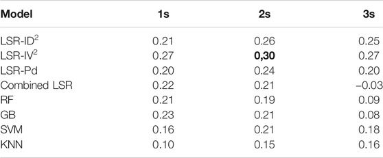
TABLE 9. R² scores for US dataset corrected drift prediction.

The best model after the $D{r}_M$ correction is the LSR with IV²_2s. As anticipated, this is the reason why we plotted the result for this model in Figure 6.

By construction, after the magnitude correction, the error-bars (green) have all zero-mean, but we can see that also the residuals for the test set are consistent with zero (Figure 6C). Figure 6A now shows that residuals for the training set have the same number of buildings with underestimated and overestimated predictions. Moreover, the residuals for the testing set are consistent the training one, but for three buildings (i.e., “14,654”, “54,341”, and “58,776”). This variability well agrees with Figure 5A and as discussed, it depends on site and buildings effects. In Figure 6B, for both training and testing set, we find again the difference in mean residuals for low-rize and high-rize buildings, but this effect is present especially for ST buildings. Moreover, the drift for high-rize ST buildings is now meanly overestimated. In the end, in Figure 6D, we see that, despite some oscillation, the residuals have not any more dependence with distance, as seen for Japanese buildings in Figure 5D.

As conclusion of this analysis, we can state that when the models retrieved considering the Japanese dataset are applied to the U.S. dataset, the Dr. predictions present a severe bias. However, by including a magnitude dependent correction term seems a relatively simple and practice solution to solve the problem. We have also found that the LSR models, after the correction, perform better than ML models. The best model, in this case, is the LSR with IV²_2s.

Conclusion

In this work, we tested the performance of several predicting models for building drift using three different EEW P-wave parameters computed considering three time-window lengths, for a total of nine features. We used a dataset of almost 6,000 waveforms from in-building sensors recorded in Japan and California. We compared linear least square and non-linear machine learning regressions for a total of 21 different models. We set up four different case-studies to understand how the data variability affects the predictions.

Our results can be summarized as follow:

Analyzing a single building (“ANX”) with a very long history of records, then all the data for the steel-reinforced concrete buildings (which contains “ANX”), and finally the entire Japanese dataset, we show that the training and the testing set have the same kind of variability and ML models perform always better than least square regression. In particular, ML models result more efficient in dealing with the non-linearity of the problem, likely because they are able to get more information from features combining them together. Moreover, the results prove that the increasing of the time window always improves the predictions. The results showed us that it is possible to retrieve building specific EEW models for Dr. prediction. This result is probably also related to the large size and good quality of the ANX dataset.

The results for the steel-reinforced concrete buildings dataset show that we can retrieve reliable models also grouping data from similar buildings. Having a lot of data from more buildings can help to overcome the problems of a few data from a single building, but at the price of a decrease in the accuracy of the predictions. Indeed, we observed a further reduction in accuracy when we used the entire Japanese dataset. So, increasing in variability of the dataset lead to models prone to precision of the predictions problems that should be considered accurately.

To better understand this issue, we used models retrieved on the entire dataset to explore the residuals correlation with buildings, types of construction, magnitude, and distance. This analysis has shown that the prediction residuals are strongly dependent from buildings and magnitude. In particular, we have found that some buildings are not well described by the models. This effect can be considered as a site-effects, which is in this application due to effects of many combined factors (e.g., 1D-to-3D soil amplification, soil-structure interaction, building resonance). Instead, looking at the magnitude, we observed a drift overestimation at lower magnitude (M < 4) and an underestimation at higher magnitude (M > 7.5). Such latter effect is the more worrying for EEW applications and it is likely due to both the lack of data in this range of larger magnitude, and to the time window length of 3s that does not contain enough information about the source size.

We have applied the Japanese models to predict the Dr. in U.S. buildings, and we have found that in this case the predictions are biased leading Dr. being underestimated. An important warning from our study is that EEW models for drift prediction are not directly exportable. This bias may be mainly due to geological and seismological differences between Japan and California. An analysis of residuals decomposed for different factors has shown a strong dependency from site-effects and magnitude.

We proposed a method to correct the prediction bias resulting from exporting EEW model to other regions from those of calibration. We showed that by applying a magnitude dependent correction terms to the predictions the biases can be removed. Hence, we showed that by the suggested method, the predictions become reliable again.

Finally, an interesting result is that, in the particular case of exporting models to another region, the linear models perform better than machine learning. This result, despite is not very surprising since it is well-known that the non-linear models are less able to extrapolate predictions outside the features’ domain of the training set, can be a useful warning for the EEWS community approaching to ML regressors.

Future studies will explore the application of the proposed methodology considering dataset from different regions. For those areas characterized by very large earthquakes, as Japan or Chile, we will explore the use of larger P-wave time-windows. We believe that this study can stimulate applications of non-linear ML models in the on-site EEW framework. Indeed, future studies can use similar approaches for the computation of ground motion parameters (i.e., PGV, PGA, etc.), as well as of other engineering demand parameters.

A final key point coming out from our analysis is the importance to better understand how the inner variability of a dataset affects the predictions. Our results suggest in fact that by increasing the datasets, we can improve the characterization of the prediction variability ascribed to site effects (e.g. soil-conditions, building response, soil to structure interaction, etc.).

Data Availability Statement

The pre-processed data supporting the conclusion of this article will be made available by the authors, without undue reservation.

Author Contributions

AI made most of the analysis and wrote the first draft. PG provided the dataset. SG organized the database. All authors contributed to conception and design of the study. All authors contributed to manuscript revision, read, and approved the submitted version.

Funding

AI was funded by the “Programma Operativo Nazionale FSE-FESR Ricerca e Innovazione” (PON FSE-FESR RI) 2014-2020. PG and SG were funded by the URBASIS-EU project (H2020-MSCA-ITN-2018, grant number 813137). Part of this work (PG) was supported by the Real-time earthquake rIsk reduction for a reSilient Europe (RISE) project, funded by the EU Horizon 2020 program under Grant Agreement Number 821115.

Conflict of Interest

The authors declare that the research was conducted in the absence of any commercial or financial relationships that could be construed as a potential conflict of interest.

Supplementary Material

The Supplementary Material for this article can be found online at: https://www.frontiersin.org/articles/10.3389/feart.2021.666444/full#supplementary-material

References

Altman, N. S. (1992). An Introduction to Kernel and Nearest-Neighbor Nonparametric Regression. The Am. Statistician 46, 175–185. doi:10.1080/00031305.1992.10475879
Astorga, A., Guéguen, P., Ghimire, S., and Kashima, T. (2020). NDE1.0: a New Database of Earthquake Data Recordings from Buildings for Engineering Applications. Bull. Earthquake Eng. 18, 1321–1344. doi:10.1007/s10518-019-00746-6
Astorga, A., Guéguen, P., and Kashima, T. (2018). Nonlinear Elasticity Observed in Buildings during a Long Sequence of Earthquakes. Bull. Seismol. Soc. Am. 108, 1185–1198. doi:10.1785/0120170289
Astorga, A. L., Guéguen, P., Rivière, J., Kashima, T., and Johnson, P. A. (2019). Recovery of the Resonance Frequency of Buildings Following strong Seismic Deformation as a Proxy for Structural Health. Struct. Health Monit. 18, 1966–1981. doi:10.1177/1475921718820770
Atik, L. A., Abrahamson, N., Bommer, J. J., Scherbaum, F., Cotton, F., and Kuehn, N. (2010). The Variability of Ground-Motion Prediction Models and its Components. Seismological Res. Lett. 81 (5), 794–801. doi:10.1785/gssrl.81.5.794
Brondi, P., Picozzi, M., Emolo, A., Zollo, A., and Mucciarelli, M. (2015). Predicting the Macroseismic Intensity from Early Radiated P Wave Energy for On-Site Earthquake Early Warning in Italy. J. Geophys. Res. Solid Earth 120, 7174–7189. doi:10.1002/2015JB012367
Caruso, A., Colombelli, S., Elia, L., Picozzi, M., and Zollo, A. (2017). An On-Site Alert Level Early Warning System for Italy. J. Geophys. Res. Solid Earth 122, 2106–2118. doi:10.1002/2016JB013403
Chan, R. W. K., Lin, Y.-S., and Tagawa, H. (2019). A Smart Mechatronic Base Isolation System Using Earthquake Early Warning. Soil Dyn. Earthquake Eng. 119, 299–307. doi:10.1016/j.soildyn.2019.01.019
Chung, A. I., Meier, M.-A., Andrews, J., Böse, M., Crowell, B. W., McGuire, J. J., et al. (2020). Shakealert Earthquake Early Warning System Performance during the 2019 ridgecrest Earthquake Sequence. Bull. Seismol. Soc. Am. 110, 1904–1923. doi:10.1785/0120200032
Cortes, C., and Vapnik, V. (1995). Support-vector Networks. Mach. Learn. 20, 273–297. doi:10.1007/bf00994018
D’Errico, L., Franchi, F., Graziosi, F., Marotta, A., Rinaldi, C., Boschi, M., et al. 2019, Structural Health Monitoring and Earthquake Early Warning on 5g Urllc Network, in IEEE 5th World Forum on Internet of Things, WF-IoT 2019 - Conference Proceedings.
Dietterich, T. (1995). Overfitting and Undercomputing in Machine Learning. ACM Comput. Surv. 27, 326–327. doi:10.1145/212094.212114
Fleming, K., Picozzi, M., Milkereit, C., Kuhnlenz, F., Lichtblau, B., Fischer, J., et al. (2009). The Self-Organizing Seismic Early Warning Information Network (SOSEWIN). Seismological Res. Lett. 80, 755–771. doi:10.1785/gssrl.80.5.755
Friedman, J. H. (2001). Greedy Function Approximation: A Gradient Boosting Machine. Ann. Statist. 29. doi:10.1214/aos/1013203451
Gasparini, P., Manfredi, G., and Zschau, J. (2011). Earthquake Early Warning as a Tool for Improving Society's Resilience and Crisis Response. Soil Dyn. Earthquake Eng. 31, 267–270. doi:10.1016/j.soildyn.2010.09.004
Ghimire, S., Guéguen, P., and Astorga, A. (2021). Analysis of the Efficiency of Intensity Measures from Real Earthquake Data Recorded in Buildings. Soil Dyn. Earthquake Eng. 147, 106751. doi:10.1016/j.soildyn.2021.106751
Guéguen, P., Johnson, P., and Roux, P. (2016). Nonlinear Dynamics Induced in a Structure by Seismic and Environmental Loading. The J. Acoust. Soc. America 140, 582–590. doi:10.1121/1.4958990
Hoshiba, M., Iwakiri, K., Hayashimoto, N., Shimoyama, T., Hirano, K., Yamada, Y., et al. (2011). Outline of the 2011 off the Pacific Coast of Tohoku Earthquake (M W 9.0) -Earthquake Early Warning and Observed Seismic Intensity-. Earth Planet. Sp 63 (7), 547–551. doi:10.5047/eps.2011.05.031
Iaccarino, A. G., Picozzi, M., Bindi, D., and Spallarossa, D. (2020). Onsite Earthquake Early Warning: Predictive Models for Acceleration Response Spectra Considering Site Effects. Bull. Seismol. Soc. Am. 110 (3), 1289–1304. doi:10.1785/0120190272
Kubo, T., Hisada, Y., Murakami, M., Kosuge, F., and Hamano, K. (2011). Application of an Earthquake Early Warning System and a Real-Time strong Motion Monitoring System in Emergency Response in a High-Rise Building. Soil Dyn. Earthquake Eng. 31, 231–239. doi:10.1016/j.soildyn.2010.07.009
Lin, Y.-S., Chan, R. W. K., and Tagawa, H. (2020). Earthquake Early Warning-Enabled Smart Base Isolation System. Automation in Construction 115, 103203. doi:10.1016/j.autcon.2020.103203
Luco, N. (2002). Probabilistic Seismic Demand Analysis, SMRF Connection Fractures, and Near-Source Effects. Stanford University.
Mignan, A., and Broccardo, M. (2019). One Neuron versus Deep Learning in Aftershock Prediction. Nature 574, E1–E3. doi:10.1038/s41586-018-0438-y
Minson, S. E., Baltay, A. S., Cochran, E. S., Hanks, T. C., Page, M. T., McBride, S. K., et al. (2019). The Limits of Earthquake Early Warning Accuracy and Best Alerting Strategy. Sci. Rep. 9–1. doi:10.1038/s41598-019-39384-y
Mousavi, S. M., and Beroza, G. C. (2020). A Machine‐Learning Approach for Earthquake Magnitude Estimation. Geophys. Res. Lett. 47. doi:10.1029/2019GL085976
Olivieri, M., Allen, R. M., and Wurman, G. (2008). The Potential for Earthquake Early Warning in Italy Using ElarmS. Bull. Seismological Soc. America 98 (1), 495–503. doi:10.1785/0120070054
Picozzi, M. (2012). An Attempt of Real-Time Structural Response Assessment by an Interferometric Approach: A Tailor-Made Earthquake Early Warning for Buildings. Soil Dyn. Earthquake Eng. 38, 109–118. doi:10.1016/j.soildyn.2012.02.003
Pinheiro, J. C., and Bates, D. M. (2000). Mixed-Effects Models in S and S-Plus: Statistics and Computing. Switzerland: Springer Nature. doi:10.1007/978-1-4419-0318-1
Raschka, S., and Mirjalili, V. (2017). Python Machine Learning: Machine Learning and Deep Learning with Python, Scikit-Learn, and TensorFlow. 2nd Edition Packt Publishing
Satriano, C., Wu, Y.-M., Zollo, A., and Kanamori, H. (2011). Earthquake Early Warning: Concepts, Methods and Physical Grounds. Soil Dyn. Earthquake Eng. 31, 106–118. doi:10.1016/j.soildyn.2010.07.007
Spallarossa, D., Kotha, S. R., Picozzi, M., Barani, S., and Bindi, D. (2019). On-site Earthquake Early Warning: A Partially Non-ergodic Perspective from the Site Effects point of View. Geophys. J. Int. 216 (2), 919–934. doi:10.1093/gji/ggy470
Stafford, P. J. (2014). Crossed and Nested Mixed-Effects Approaches for Enhanced Model Development and Removal of the Ergodic assumption in Empirical Ground-Motion Models. Bull. Seismological Soc. America 104, 702–719. doi:10.1785/0120130145
Stone, M. (1974). Cross-validation and Multinomial Prediction. Biometrika 61, 509–515. doi:10.1093/biomet/61.3.509
Strauss, J. A., and Allen, R. M. (2016). Benefits and Costs of Earthquake Early Warning. Seismological Res. Lett. 87, 765–772. doi:10.1785/0220150149
Tubaldi, E., Ozer, E., Douglas, J., and Gehl, P. (2021). Examining the Contribution of Near Real-Time Data for Rapid Seismic Loss Assessment of Structures. Struct. Health Monit., 147592172199621. doi:10.1177/1475921721996218
van de Geer, J. P. (1995). Some Aspects of Minkowski Distance. Leiden, Netherlands: Leiden University, Department of Data Theory, Esearch report.
Wu, Y.-M., and Kanamori, H. (2008). Development of an Earthquake Early Warning System Using Real-Time strong Motion Signals. Sensors 8, 1–9. doi:10.3390/s8010001
Wu, Y.-M., and Kanamori, H. (2005). Experiment on an Onsite Early Warning Method for the Taiwan Early Warning System. Bull. Seismological Soc. America 95, 347–353. doi:10.1785/0120040097
Yamada, M., and Mori, J. (2009). Using τC to Estimate Magnitude for Earthquake Early Warning and Effects of Near-Field Terms. J. Geophys. Res. 114, B05301–353. doi:10.1029/2008JB006080
Keywords: earthquake early warning, onsite EEW, structural drift, machine learning regressors, building monitoring
Citation: Iaccarino AG, Gueguen P, Picozzi M and Ghimire S (2021) Earthquake Early Warning System for Structural Drift Prediction Using Machine Learning and Linear Regressors. Front. Earth Sci. 9:666444. doi: 10.3389/feart.2021.666444
Received: 10 February 2021; Accepted: 21 June 2021;
Published: 08 July 2021.
Edited by:
Maren Böse, ETH Zurich, SwitzerlandReviewed by:
Stephen Wu, Institute of Statistical Mathematics (ISM), JapanEnrico Tubaldi, University of Strathclyde, United Kingdom
Copyright © 2021 Iaccarino, Gueguen, Picozzi and Ghimire. This is an open-access article distributed under the terms of the Creative Commons Attribution License (CC BY). The use, distribution or reproduction in other forums is permitted, provided the original author(s) and the copyright owner(s) are credited and that the original publication in this journal is cited, in accordance with accepted academic practice. No use, distribution or reproduction is permitted which does not comply with these terms.
*Correspondence: Antonio Giovanni Iaccarino, antoniogiovanni.iaccarino@unina.it