An Efficient Algorithm for Retrieving CO₂ in the Atmosphere From Hyperspectral Measurements of Satellites: Application of NLS-4DVar Data Assimilation Method

Introduction

The concentration of CO₂ in the atmosphere has continued to increase since the Industrial Revolution, which has had a significant impact on the global climate (Cox et al., 2000; Le Quéré et al., 2016). The formulation of climate policy and control of the future climate require a more accurate and comprehensive understanding of the global carbon cycle (Dilling et al., 2003). Current ground-based and aircraft observations could provide help in modelling and understanding global sources and sinks of CO₂ (Wunch et al., 2011); however, the insufficient number and sparse spatial coverage make it difficult to obtain accurate CO₂ fluxes on regional scales (Baker et al., 2010; O'Dell et al., 2012).

To acquire CO₂ fluxes with high spatial and temporal resolutions to supplement the deficiencies of ground-based and aircraft observations, efforts have been made to retrieve the column-averaged dry air mole fraction of atmospheric CO₂ (X_CO2) from satellite observations (Rayner and O'Brien, 2001; Miller et al., 2007). Data retrieved from the thermal infrared spectrograph are able to provide good information of CO₂ in the mid-troposphere (Chédin et al., 2003; Crevoisier et al., 2009; Kulawik et al., 2010), but the measurements are less sensitive to near surface CO₂ variations. Therefore measurements in Near-infrared (NIR)- and short-wave infrared (SWIR)-band are proposed, such as the SCanning Imaging Absorption spectroMeter for Atmospheric CHartographY (SCIAMACHY) (Buchwitz et al., 2005; Reuter et al., 2011), which is a mid-resolution spectrometer. The first dedicated greenhouse gas satellite Greenhouse gases Observing SATellite (GOSAT) and its successor GOSAT-2, with ultra-high spectral resolution in NIR and SWIR bands, were launched into space by Japan Erospace Exploration Agency (JAXA) separately in 2008 (Yokota et al., 2009) and 2018 (Nakajima et al., 2012). Similar specific satellites such as Orbiting Carbon Observatory-2 (OCO-2) (Crisp et al., 2004) and OCO-3 (Eldering et al., 2019) are launched into space separately in 2014 and 2019. China also launched its first satellite, TanSat, for Carbon dioxide measurements in 2016 (Yang et al., 2018). These measurements from space could provide spatial map of atmospheric CO₂ and its variation both on regional and global scales (Jiang and Yung, 2019).

A variety of algorithms have been developed for retrievals of CO₂ from NIR and SWIR spectra, including the Differential Optical Absorption Spectroscopy (DOAS) approach for SCIAMACHY (Buchwitz et al., 2000; Honninger et al., 2004; Reuter et al., 2010), the National Institute for Environment Studies (NIES) algorithm developed for GOSAT measurements (Yoshida et al., 2011), the Atmospheric CO₂ Observations from Space (ACOS) algorithm applied to GOSAT and OCO-2 measurements (Crisp et al., 2012; O'Dell et al., 2012; O'Dell et al., 2018), the University of Leicester Full Physics (UoL-FP) algorithm (Boesch et al., 2011), the RemoTeC algorithm developed by SORN Netherlands Institute for Space Research and Deutsches Zentrum für Luft-und Raumfahrt e.V. (DLR) (Hasekamp and Butz, 2008; Butz et al., 2011; Guerlet et al., 2013) and the ensemble median (EEMA) algorithm (Reuter et al., 2013).

Until now, it is still a challenge to retrieve accurate CO₂ concentrations and its vertical profiles from satellite measurements (Yue et al., 2016), some of them can only produce reasonable results under very clear skies. This is due to limitations of parameterization and simplification in the algorithm, i.e., first guess of CO₂ profile, atmospheric parameters and their vertical distributions, and simplification of the weighting function matrix calculation owing to time-consuming burden. In this paper, a novel algorithm, NLS-4DVar-based CO₂ Retrieval Algorithm (NARA), is proposed. The NLS-4DVar method rewrites the cost function as a nonlinear least squares problem and solves it iteratively using the Gauss-Newton method. In the iterative process, the a priori covariance matrix is not a fixed one but constantly updated. Moreover, the calculations of the weighting function matrix and its transposition are avoided through simple mathematical transformations, which greatly reduces programming difficulty and computational complexity while maintaining the retrieval accuracy. This is particularly important for space-based CO₂ retrievals considering the huge number of satellite measurements.

The rest of this article is organized as follows. Sect. 2 introduces the NARA algorithm in detail, including the forward and inverse models. Sect. 3 evaluates the NARA algorithm in terms of X_CO2 and the CO₂ profile through observing system simulation experiments (OSSEs). Sect. 4 describes real-data retrievals using OCO-2 observations and comparisons between NARA retrieved X_CO2 and coincident TCCON measurements. Finally, Sect. 5 discusses and concludes the paper.

Description of the NLS-4DVar-based CO₂ Retrieval Algorithm

The NARA retrieval algorithm obtains the optimal state vector under the joint constraints of satellite measurements and prior information. The state vector contains the CO₂ profile and several parameters to which the spectra are sensitive. The optimal column-averaged CO₂ is calculated according to the CO₂ profile. The NARA algorithm can be applied to any greenhouse gas satellites, but requires some specific modifications according to the satellite instruments. At present, we use information and observations from OCO-2 satellite to make preliminary evaluations of the NARA algorithm. The OCO-2 observations of the reflected sunlight spectra in three bands: O₂ A band at 0.76 µm, weak CO₂ band at 1.61 µm, and strong CO₂ band at 2.06 µm are used for retrievals (O'Dell et al., 2018). NARA algorithm include data preparation, X_CO2 retrieval and bias correction. A flow chart of the NARA algorithm is shown in Figure 1.

1. Data Input and Pre-screening

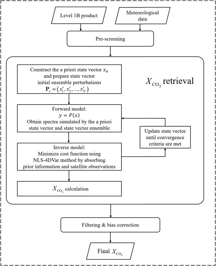
FIGURE 1. Flow chart of the NARA algorithm.

The input data of the algorithm include the Level 1B product of satellite measurements and meteorological data interpolated to the observation points. The Level 1B product includes the calibrated radiances for three spectral bands and geolocation information. The pixels with low signal-to-noise ratio and those contaminated by clouds and aerosols are filtered out (Taylor et al., 2016). The meteorological data include surface pressure, water vapor profile, temperature profile, and surface wind speed, which are from gridded GEOS5-FP-IT (Goddard Earth Observing System, Version 5, Forward Processing for Instrument Teams) reanalysis and interpolated to the observation location.

2. X_CO2 Retrieval

The X_CO2 retrieval is the core of the algorithm. X_CO2 is the column-averaged dry air mole fraction of atmospheric CO₂, and the unit is part per million (ppm). The a priori state vector from the input data, as well as the initial ensemble of the state vector, are constructed. They are then input into the forward model to obtain simulated spectra. This information and satellite observations are input into the inverse model, and the optimal estimate of the state vector is obtained through the NLS-4DVar method. X_CO2 is then calculated according to the CO₂ profile in the state vector.

3. Bias Correction

Currently all space-borne X_CO2 retrievals have systematic biases, mainly due to uncertainty in spectroscopy, limitations in the information provided by the observations, imperfect modelling of the atmosphere and surface, as well as uncertainty in instruments. Therefore, bias correction is necessary for the retrieved X_CO2 (Schneising et al., 2012; Guerlet et al., 2013; Crisp et al., 2017). The bias correction procedure of NARA algorithm adopted from OCO-2 consists of three main parts: first, correct the parametric biases that is caused by the spurious correlation of the retrieved X_CO2 with other retrieval parameters; second, correct the footprint-dependent biases that are truly instrument-related; finally, apply a global scaling to remove the remaining biases (O'Dell et al., 2018).

Forward Model

The parameters to be optimized in the forward model constitute the state vector $\mathit{x}$. The reflected sunlight received by all channels in the three bands constitutes the observation vector $\mathit{y}$. The simulation of observation from a state vector can be expressed by the following formula:

where $F$ is the forward model, $\mathit{b}$ is a set of fixed input parameters, and $\mathbf{\epsilon }$ is the error in both the instrument and forward model. The forward model uses the Linearized Discrete Ordinate Radiative Transfer (LIDORT) model (Spurr et al., 2001; Spurr and Natraj, 2011) as the radiative transfer model and some parameters about solar, surface and instrument provided by the ACOS algorithm (O'Dell et al., 2018). The state vector includes the CO₂ profile defined at a set of 20 atmospheric pressure levels, a temperature profile offset, surface pressure, a water vapor profile multiplier, aerosol parameters, surface albedo parameters, instrument correction parameters, spectrum correction parameters, and solar-induced fluorescence (SIF) parameters, which are listed in Table 1 in detail. The atmosphere with few clouds and aerosols can retrieve more accurate X_CO2 than other conditions because of atmospheric scattering. To account for scattering effects of thin clouds and aerosols, the retrieval solves simultaneously for amounts and Gaussian vertical profiles of five different kinds of scatterers with fixed optical properties: a water cloud type, an ice cloud type, two fixed aerosol types, and an upper tropospheric / lower stratospheric sulfate aerosol type. The two fixed aerosol types are chosen from co-located GEOS-5 FP-IT aerosols. They are the types that form the highest and second highest fraction of the AOD (aerosol optical depth) at 755 nm for a co-located GEOS-5 grid cell for a given sounding.

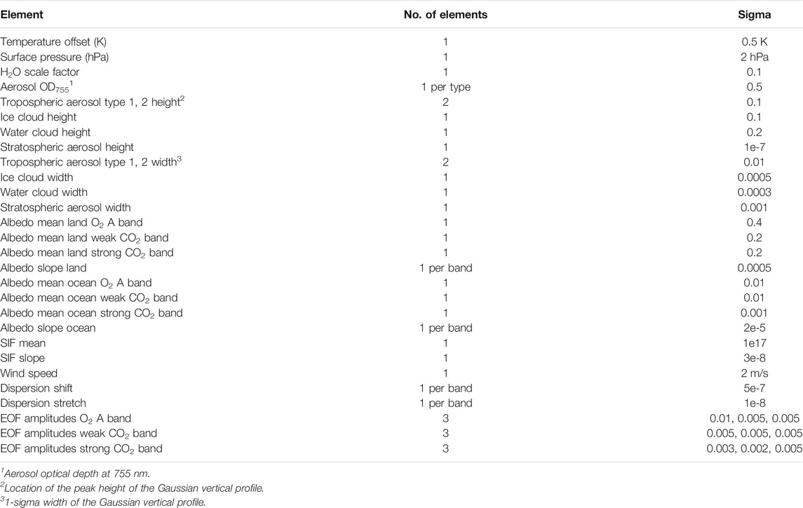
TABLE 1. Standard deviations of normal distributions when generating ensembles of initial perturbations for parameters in the state vector excluding the CO₂ profile.

The prior value of the state vector is calculated by the ACOS algorithm (O'Dell et al., 2012; O'Dell et al., 2018). The vertical coordinate uses a simple sigma coordinate system, that is ${\mathit{P}}_{\text{levels}}={\mathit{P}}_{\text{surf}}\cdot \mathit{a}$, $\mathit{a}={\left(0.0001,\frac{1}{19},\frac{2}{19},\dots ,\frac{18}{19},1\right)}^T$, where ${\mathit{P}}_{\text{levels}}$ is the 20 vertical pressure levels, ${\mathit{P}}_{\text{surf}}$ is the surface pressure, and $\mathit{a}$ is a fixed coefficient array. For ${\mathit{P}}_{\text{surf}}=1000 \text{hPa}$, the pressure width of all the layers (except the top layer) is 52.63 h Pa; for the top layer it is 52.53 hPa. The typical model lid is roughly 0.1 hPa. Assume that the tropopause pressure is 200 hPa (Hoinka, 1998), then the ratio of the tropopause pressure to the surface pressure is 0.2. According to the $\mathit{a}$ coefficient, the CO₂ profile mainly describes the troposphere CO₂ concentration, apart from about the first four levels describing the CO₂ concentration above the troposphere.

Inverse Model

The inverse model is used to obtain the minimum value of the following cost function through the optimization algorithm:

where ${\mathit{x}}_{\mathbf{a}}\in {\mathrm{ℝ}}^{n_x}$ ($n_x$ is the dimension of the state vector) is the a priori state vector, ${\mathbf{S}}_{\mathbf{a}}$ is the a priori covariance matrix, $F\left(\mathit{x}\right)$ is the spectra simulated by the state vector, ${\mathbf{S}}_{\mathbf{\epsilon }}$ is the observation error covariance matrix, and the superscript $\text{T}$ stands for the matrix transposition. The NARA algorithm uses the NLS-4DVar method to minimize the cost function.

NLS-4DVar Method

The NLS-4DVar method (Tian and Feng, 2015; Tian et al., 2018) rewrites the cost function in Eq. 2 into an incremental format to determine the analysis increment for the a priori state vector:

where $\mathit{x}\prime =\mathit{x}-{\mathit{x}}_a$ is the perturbation of the prior field ${\mathit{x}}_a$, $\mathit{y}\in {\mathrm{ℝ}}^{n_y}$, and $n_y$ is the dimension of the observation. To avoid the direct inversion of the a priori covariance matrix ${\mathbf{S}}_a$, the NLS-4DVar method expresses the analysis increment $\mathit{x}{\prime }^{,\ast }$ as a linear combination of the initial perturbations:

where ${\mathbf{P}}_{\mathit{x}}=\left(\mathit{x}{\mathrm{\prime }}_{\mathrm{1}},\mathit{x}{\mathrm{\prime }}_{\mathrm{2}},\dots ,\mathit{x}{\mathrm{\prime }}_{\mathrm{N}}\right)$ is the ensemble of prepared initial perturbations, ${\mathit{x}}_j^{\prime }={\mathit{x}}_j-{\mathit{x}}_a\left(j=\mathrm{1,2},\dots ,N\right)$ is the jth perturbation, N is the ensemble size, and $\mathit{\beta }={\left({\beta }_1,{\beta }_2,\dots ,{\beta }_N\right)}^{\text{T}}$ is the coefficient vector. A reasonable ensemble of perturbations ${\mathbf{P}}_{\mathit{x}}$ can provide an appropriate solution space for the analysis increment $\mathit{x}{\prime }^{,\ast }$. We further assume that the a priori covariance matrix can be approximated by the ensemble covariance matrix ${\mathbf{B}}_e$, that is, ${\mathbf{S}}_a\approx {\mathbf{B}}_e=\left({\mathbf{P}}_x\right){\left({\mathbf{P}}_x\right)}^{\text{T}}/N-1$. As the ensemble of perturbations is updated with iterations, the a priori covariance matrix ${\mathbf{S}}_a$ will also be updated. Compared with the general methods that use a fixed ${\mathbf{S}}_a$, this constantly updated ${\mathbf{S}}_a$ tends to be more precise as the iteration progresses. Substituting the above assumptions into Eq. 3 yields

Obviously, Eq. 7 can be solved iteratively by computing the cost function and its gradient:

where $\mathbf{K}=\partial F\left(\mathit{x}\right)/\partial \mathit{x}$ is the weighting function matrix (tangent linear model) and ${\left(\mathbf{K}\right)}^{\text{T}}$ is the transposition of the weighting function matrix (adjoint model). The programming difficulty and computational complexity of the weighting function matrix and its transposition are huge; combined with the large number of satellite measurements, this greatly increases the computational cost. This is a problem faced by some other algorithms (Connor et al., 2008; Butz et al., 2009; Yoshida et al., 2011; Butz et al., 2012; Cogan et al., 2012).

To circumvent the calculation of the weighting function matrix and its transposition, the NLS-4DVar method converts Eq. 7 into the following nonlinear least squares problem:

Here $\left({\mathbf{S}}_{\epsilon ,+}^{1/2}\right){\left({\mathbf{S}}_{\epsilon ,+}^{1/2}\right)}^{\mathrm{T}}={\mathbf{S}}_{\epsilon }$. The Gauss-Newton iteration method (Dennis and Schnabel, 1996) is used to minimize the cost function. After a simple mathematical derivation, the optimal state vector is obtained without calculating the weighting function matrix and its transposition, which is shown in Appendix A. The final formula is given below (Tian et al., 2018):

where ${\mathit{y}}^{\prime ,i-1}=\mathit{y}-F\left({\mathit{x}}^{i-1,\ast }\right)$, ${\mathit{x}}^{i-1,\ast }$ is the optimal analysis of the state vector in the last step, and

where

According to Tian et al. (2018), the cost function generally reaches the minimum convergence standard after three iterations. Here the optimal state vector contains the CO₂ profile component, allowing the calculation of the best estimation of X_CO2.

Initial Ensemble Generation

As mentioned above, the NLS-4DVar method assumes that the analysis increment can be expressed as the linear combination of the initial perturbations; the quality of the initial ensemble of perturbations is vital to the success of the retrieval. For different components in the state vector, we use different initial ensemble generation methods. The CO₂ profile ensemble of perturbations is generated by the random state variable (RSV) method (Zhang, 2019), the ensembles of the other components are generated by normal distributions.

The RSV method first requires a big ensemble of perturbations. The method then performs singular value decomposition and the random orthogonal matrix to obtain the final small ensemble (Evensen, 2009). The big ensemble comes from the model simulated CO₂ of GEOS-Chem (v11-01; http://acmg.seas.harvard.edu/geos/). There are seven carbon fluxes used to drive GEOS-Chem: fossil fuel emissions, ocean carbon fluxes, terrestrial ecosystem fluxes, biomass burning emissions, ships emissions, aviation emissions, and chemical oxidation production. The ocean carbon fluxes and terrestrial ecosystem fluxes are optimized by the Tan-Tracker flux inversion system (Tian et al., 2014a; Tian et al., 2014b) through assimilating OCO-2 X_CO2 retrievals. GEOS-Chem simulates the CO₂ profile at 47 atmospheric pressure levels, with a horizontal resolution of 2° latitude × 2.5° longitude. The 47 pressure levels are defined using the hybrid sigma-pressure grid, and the top atmospheric pressure level is about 0.038 hPa (http://wiki.seas.harvard.edu/geos-chem/index.php/GEOS-Chem_vertical_grids#Hybrid_grid_definition, last access: June 3, 2021). In order to avoid the size of big ensemble being too large, the CO₂ profile is taken every 4 grid points along the longitude and the daily average CO₂ profile is computed. The profile is then interpolated to the 20 pressure levels, where the CO₂ profile in the NARA algorithm is located. According to the month and latitude of the satellite measurement, the model data of the two latitude bands above and below the measurement latitude during an entire month are selected as the big ensemble. For example, consider the measurement at 36.641° N and 97.441° W on January 30, 2016. The simulation results of GEOS-Chem at 36.0° N and 38.0° N in January 2016 show a total of $36\times 2\times 31=2232$ CO₂ profiles, which constitute the big ensemble after subtraction of the a priori CO₂ profile, denoted by ${\mathbf{C}}_e$. Singular value decomposition of ${\mathbf{C}}_e$ yields

where $\mathbf{U}\in {ℝ}^{n_x\times n_x}$, ${\displaystyle \sum \in {\mathrm{ℝ}}^{n_x\times \alpha N}}$, and $\mathbf{V}\in {ℝ}^{\alpha N\times \alpha N}$.

Here ${\mathbf{C}}_s$ is the initial ensemble, $1\le \gamma \le \alpha$ and $\mathbf{\Theta }\in {ℝ}^{N\times \gamma N}$ (Evensen, 2009). $\mathbf{\Theta }$ is a random matrix and has orthonormal rows, which can be constructed by extracting the first N rows of the random orthogonal matrix $\mathbf{\Theta }\in {ℝ}^{\gamma N\times \gamma N}$ (Evensen, 2009). Adding the a priori CO₂ profile to the initial ensemble, we obtain the initial CO₂ profiles.

The initial ensembles of the other parameters in the state vector are the random perturbations of normal distributions; that is, the mean of the normal distribution takes the prior value. The standard deviations (Table 1) were obtained by sensitivity experiments and analysing OCO-2 data. The initial ensemble of the state vector is constructed by combining the CO₂ profile ensemble and the remaining parameter ensembles together. Add the a priori state vector to the ensemble and input it into the forward model to obtain the simulated spectra. After preparing the above data, we can determine the optimal estimate of X_CO2 using the NLS-4DVar method introduced in Sect. 2.2.1.

Observing System Simulation Experiments for Evaluating the (NLS-4DVar)-based CO₂ Retrieval Algorithm

In this section, we evaluated the NARA algorithm comprehensively by performing observing system simulation experiments (OSSEs) at four different sites around the world. Besides, we conducted a set of experiments at one site, discussing the effects of aerosol amounts on X_CO2 retrievals.

Experimental Setup

A total of four sites around the world were selected for retrievals. Three were near Total Carbon Column Observing Network (TCCON) (Wunch et al., 2011) stations, specifically the Lamont (LA), Bremen (BR), and Wollongong (WO) stations, and the remaining one was on the North Pacific (OC). Information on these four sites is listed in Table 2, and their specific locations are shown in Figure 2. The impacts of surface properties, latitudes, seasons, and land–sea distribution on retrievals were carefully considered when selecting the retrieval sites to ensure the comprehensiveness of the experiments. Especially, previous studies have indicated that scenes without aerosol contamination could yield better results, and X_CO2 retrieval biases appeared to be correlated with scattering by aerosols (Wunch et al., 2017; O'Dell et al., 2018). Thus, we performed a set of OSSEs at the Lamont station to evaluate retrieval results under different aerosol amounts.

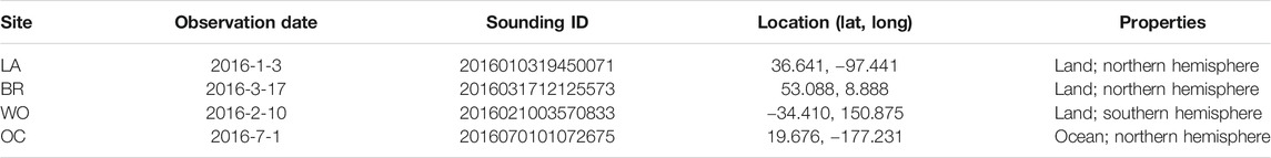
TABLE 2. Information on the four retrieval sites in the OSSEs, including the observation date, sounding ID, location (listed in degrees latitude and degrees longitude), and surface properties. (LA: Lamont; BR: Bremen; WO: Wollongong; OC: the ocean site).

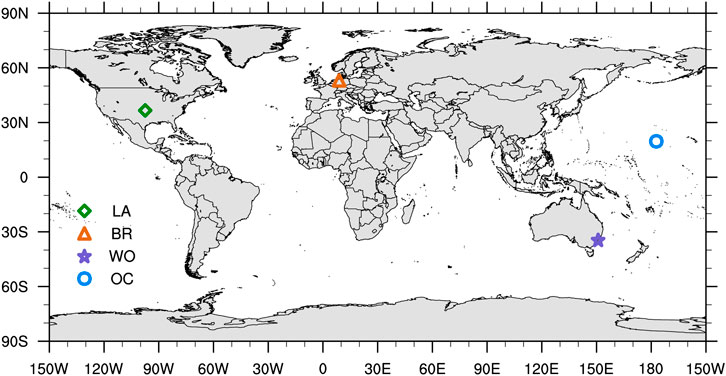
FIGURE 2. Map of the four retrieval sites in OSSEs. (LA, Lamont; BR, Bremen; WO, Wollongong; OC, the ocean site).

We used OCO-2 version eight retrospective (i.e., 8r) data in the OSSEs, including Level 1B data OCO2_L1B_Calibration 8r, meteorological data OCO2_L2_Met 8r, pre-screening data OCO2_L2_ABand 8r, and OCO2_IMAPDOAS 8r, as well as diagnostic data OCO2_L2_Diagnostic 8r (https://disc.gsfc.nasa.gov/datasets?keywords=oco2&sort=processLevel&page=1). The pre-screening procedure uses ABO₂ and IMAP-DOAS pre-processors to remove scenes contaminated by clouds or aerosols (Taylor et al., 2016). The diagnostic data provide prior and retrieved state vectors and prior X_CO2 in the OSSEs. We used target-mode data for the three retrieval sites over land and glint-mode data for the retrieval site over the ocean. We generated the initial ensemble following the method introduced in Sect. 2.2.2, and we chose 50 for the size of the ensemble after sensitivity experiments.

In OSSEs, the a priori state vector adopts the a priori value calculated by OCO-2 according to the input data, and the constructed true state vector adopts the OCO-2 retrieval result of the observation point or a nearby point. The constructed true state vector is input into the forward model to obtain the simulated spectra. The observation error of OCO-2 is then added to the simulated spectra to obtain the observation spectra. The a priori CO₂ profile and constructed true CO₂ profile are shown in Figure 6. The spectra simulated by the a priori state vector and constructed observation spectra are shown in Figure 3. For the aerosol specific evaluation, we conducted a set of OSSEs at the Lamont station on January 3, 2016 under three different tropospheric aerosol amounts. The two tropospheric aerosol types were sulfate and organic carbon. As the values of $ln\left(\text{AOD}\right)$ at 755 nm are used in the state vector, we chose three sets of $ln\left(\text{AOD}\right)$ for these two aerosols. For $ln\left(\text{AOD}\right)$ of sulfate and organic carbon, they were −4.47 and −5.97, −5.47 and −6.97, −10.47 and −11.97, respectively in the three sets.

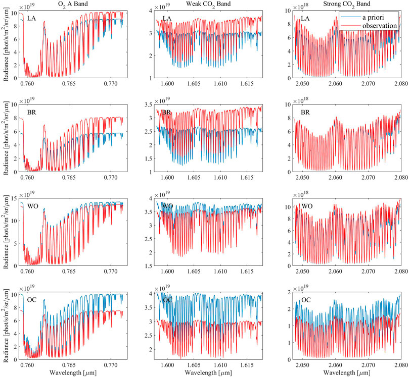
FIGURE 3. Spectra simulated by the a priori state vector and constructed observation spectra in three bands. The first column is the O₂ A band, the second column is the weak CO₂ band, and the third column is the strong CO₂ band. The first to fourth rows are the spectra at LA, BR, WO, and OC, respectively. The name of the observation point is in the upper left corner of each subplot.

Experimental Results

The retrieval quality was evaluated in terms of the X_CO2 and CO₂ profiles. X_CO2 is the product currently provided by satellite retrievals, and accurate CO₂ profiles are the goals of retrieval algorithms.

X_CO2 Results

The differences between the a priori X_CO2 and the true X_CO2 were relatively large; specifically, LA, BR, WO, and OC showed differences of 1.88, 1.70, –3.15, and 2.27 ppm, respectively. Figure 4 shows the X_CO2 obtained by the NARA algorithm after one, two, and three iterations and comparisons with the a priori X_CO2 and the true X_CO2 at the four retrieval sites. The retrieved X_CO2 gradually approached the true value as the iterations of the NARA algorithm progressed, ultimately reaching the optimal value at the third iteration. The differences between the NARA retrieved X_CO2 and the true X_CO2 after three iterations were 0.33, 0.11, 0.11, and –1.13 ppm at LA, BR, WO, and OC, respectively, which was a big improvement from the prior X_CO2 and showed that our algorithm was effective.

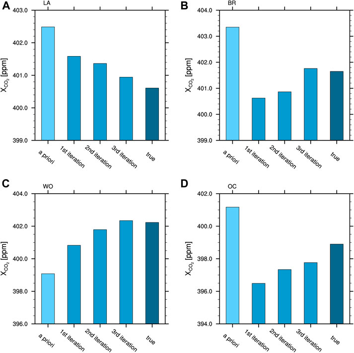
FIGURE 4. NARA retrieved X_CO2 after one, two, and three iterations and comparisons with the a prioriX_CO2 and the true X_CO2 at (A) LA, (B) BR, (C) WO, and (D) OC.

The retrievals at LA and WO were similar. At these two sites, the retrieval of the first iteration was very effective, with subsequent iterations approaching the true value. After three iterations, the NARA retrieved X_CO2 was quite close to the true X_CO2. The results for BR and OC were similar. The retrieval of the first iteration was significantly changed compared with the prior value, which showed that observation information had a huge impact on retrieval. In subsequent iterations at BR and OC, under the mutual constraints of the prior information and observations, the retrieved X_CO2 gradually approached the true value and reached the optimal X_CO2 at the third iteration. The NARA retrieved X_CO2 of the three retrieval sites over land were closer to the true X_CO2 than the NARA retrieved X_CO2 at the ocean site OC, which was attributable to the different observation modes and surface properties over land and ocean and/or the varying accuracies of the prior values.

The NARA retrieved X_CO2 depended on atmospheric AODs (Figure 5A). The prior and true X_CO2 at the observation site were 402.49 ppm and 400.61 ppm. The NARA retrieved X_CO2 for scenario 1 (S1), scenario 2 (S2), and scenario 3 (S3) were 400.94, 401.13, and 401.24 ppm, respectively. S1 had the highest AOD while S3 had the lowest AOD. It’s clear that as the AOD decreased, the bias of retrieved X_CO2 increased, which indicated that more accurate X_CO2 can be retrieved under atmospheric conditions with less aerosols.

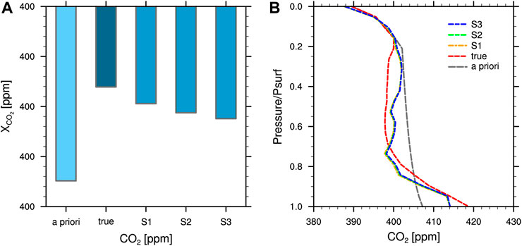
FIGURE 5. The prior and true values as well as NARA retrievals with different atmospheric AODs. (A) depicts the CO₂ profiles, and (B) depicts the X_CO2. S1, S2, and S3 indicates scenario 1, scenario 2, and scenario 3, respectively.

CO₂ Profile Results

Figure 6 shows the CO₂ profiles obtained by the NARA algorithm after one, two, and three iterations and comparisons with the a priori CO₂ profile and the true CO₂ profile at the four retrieval sites. The CO₂ profiles differed between the Northern and Southern hemispheres. The vertical gradient of the CO₂ profile in the Northern Hemisphere was larger than in the Southern Hemisphere, which is depicted in Figure 6.

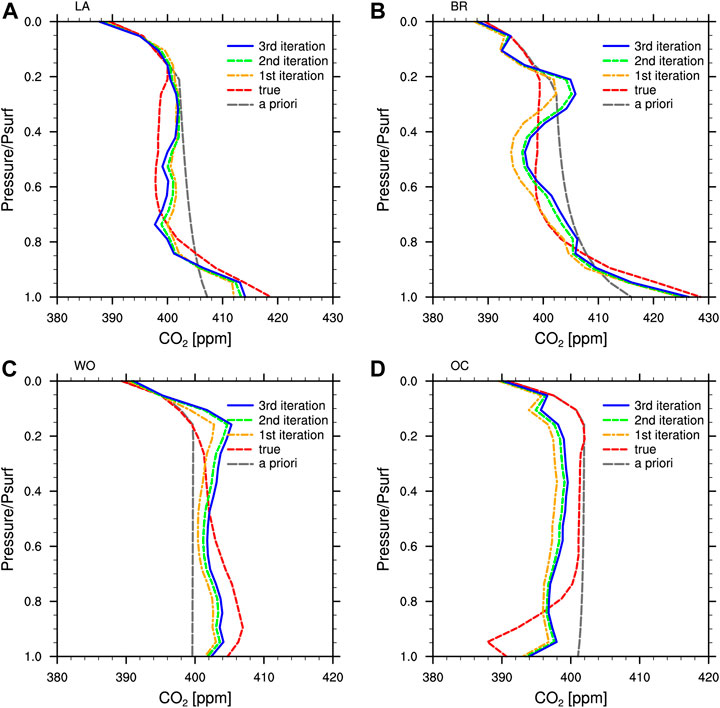
FIGURE 6. NARA retrieved CO₂ profiles after one, two, and three iterations and comparisons with a priori and true CO₂ profiles at (A) LA, (B) BR, (C) WO, and (D) OC.

First look at the retrieval results for the two Northern Hemisphere sites LA and BR. The vertical gradient of the a priori CO₂ profile was relatively small. The true CO₂ profile above the troposphere was in good agreement with the a priori CO₂ profile; however, the vertical gradient in the troposphere was greater than that of the a priori profile. As the iterations progressed, the NARA retrieved CO₂ profile gradually approached the true value. After three iterations, the NARA retrieved CO₂ profile was very close to the true profile, in particular in the lower troposphere. This is particularly important given that the carbon sources and sinks of interest are all located in the lower troposphere. A close look at the retrieval results for the two Southern Hemisphere sites WO and OC shows that the vertical gradient of the a priori CO₂ profile in the troposphere was quite small. The NARA retrieved CO₂ profiles roughly grasped the characteristics of the true profiles; however, they were unable to well simulate the relatively large vertical gradient of the true profile in the lower troposphere, which were not as good as the results for the Northern Hemisphere. Because the vertical gradient of the a priori CO₂ profile in the Southern Hemisphere was small, the vertical gradient of the CO₂ profile ensemble decomposed on the basis of the prior value was also small. The analysis increment was a linear combination of the ensemble members, thus it could not retrieve well a large vertical gradient as the true profile indicated. This problem may be solved by providing a better prior CO₂ profile. The retrieved CO₂ profile can also be influenced by aerosol contents (Figure 5B). The patterns of the CO₂ profile under different AODs were similar, but the specific CO₂ concentrations at each level were various, which contributed to the discrepancy of the column-averaged value. The above analyses demonstrate that the NARA retrieved CO₂ profiles in the Northern Hemisphere were relatively accurate, in particular in the lower troposphere. The retrieval results for the Southern Hemisphere roughly grasped the characteristics of the true profiles but still needed more improvement. The effects of aerosol scattering should also be considered during the retrievals.

Real-Data Retrievals and Comparisons With Total Carbon Column Observing Network Data

In this section, we evaluated the X_CO2 retrieved by the NARA algorithm using OCO-2 version 8r target-mode observations at two target locations and compared the NARA retrieved X_CO2 with coincident TCCON data. TCCON is a global network of ground-based instruments that can retrieve accurate and precise X_CO2, which provides an essential validation resource for space-based measurements (Wunch et al., 2011). In addition, we performed real retrievals using the normal 4DVar method, which requires the calculation of the pressure weighting function and its transposition, and compared the retrievals with NARA retrieved ones.

Experimental Setup

Target mode is designed to evaluate biases in the OCO-2 X_CO2 product, whose strength is that thousands of spectra can be obtained in a short period of time over a small region (about 0.2° latitude × 0.2° longitude for the densest measurements) (Wunch et al., 2017). The target locations are mostly selected to be coincident with ground-based stations, typically at TCCON sites (Wunch et al., 2011). Given the differences between the Northern and Southern hemispheres, the two target locations selected for validation were Lamont, Oklahoma, in the central United States and Darwin, Australia, on the northern coast. The Lamont location has relatively uniform surface properties and is reasonably far from anthropogenic CO₂ sources, and the ground cover changes with the seasons (Wunch et al., 2017); in contrast, target-mode measurements at the Darwin location contain observations over both land and ocean. Information on these two target locations is shown in Table 3. OCO-2 measurements over about 1 year were selected for validation at each of the two locations. The observation dates are listed in Table 4.

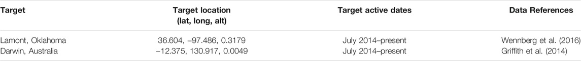
TABLE 3. Information on the two validated target locations for real retrievals. The target location is listed in degrees latitude, degrees longitude, and altitude above sea level in km.

TABLE 4. Dates of the target-mode observations selected for real retrievals at the two validated target locations.

Restricted by our computational resources, we randomly selected 10 observation points from OCO-2 pre-screened measurements for retrievals each day at the Lamont location; for the Darwin location, we randomly selected 10 observation points over land and 10 observation points over the ocean each day. For the 4DVar retrievals, we performed experiments at the Lamont station on November 24, 2014. We retrieved X_CO2 at the same 10 observation points and used the same prior values as the NARA algorithm. We assumed that TCCON data were coincident with OCO-2 target-mode measurements when they were recorded within ±30 min of the target-mode maneuver. If there were fewer than five TCCON measurements within that time frame, the period was extended to ±120 min. Then we compared the median of the NARA retrieved X_CO2 of the 10 selected observation points with the median of coincident TCCON measurements. In the real retrievals, the size of the initial ensemble was 50, and the number of iterations was three. Then we corrected the NARA retrieved X_CO2 for bias using the OCO-2 bias correction method (O'Dell et al., 2018).

Experimental Results

Figure 7 shows the median of the NARA retrieved X_CO2 and comparisons with the median of the OCO-2 retrieved X_CO2 using the ACOS algorithm for the same observation points and the median of the coincident TCCON measurements at Lamont and Darwin locations. Retrievals over the land and ocean at the Darwin location were evaluated separately because land and ocean surface reflections were modelled differently as purely Lambertian over land and Cox–Munk with a Lambertian component over water (O'Dell et al., 2018). The X_CO2 retrieved by the NARA algorithm and OCO-2 were generally smaller than TCCON data, in particular over land. It is common for OCO-2 that a retrieved X_CO2 will be smaller than TCCON data. The NARA algorithm uses similar state vector setting and aerosol characterization as the ACOS algorithm; thus, some features of NARA retrievals are similar to OCO-2 results. This problem may be mitigated by fitting an intensity offset for all three bands and improving aerosol treatments (Wu et al., 2018).

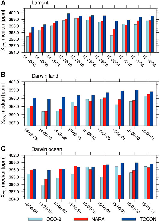
FIGURE 7. The median of the NARA retrieved X_CO2 and comparisons with median of the OCO-2 retrieved X_CO2 for the same observation points and the median of the coincident TCCON data at (A) the Lamont location, (B) the Darwin location over land, and (C) the Darwin location over the ocean.

To better evaluate the retrieval quality, we defined the bias ($b$) as the mean difference between the retrieved X_CO2 from satellite measurements and coincident TCCON data and the sounding precision ($\sigma$) as the standard deviation of the difference (Wu et al., 2018). The bias and sounding precision obtained by NARA retrievals and OCO-2 retrievals at the Lamont and Darwin locations are shown in Table 5. As shown in Figure 7 and Table 5, medians of the NARA retrieved X_CO2 were generally closer to the TCCON measurements than the OCO-2 retrievals, which demonstrates that the NARA algorithm was effective and the retrievals from NARA were comparable to those from OCO-2. For the NARA algorithm, the retrieval results (i.e., bias and sounding precision) differed at the Lamont and Darwin locations, which indicated the existence of location-dependent biases. The location dependence of the target-mode retrievals further showed that spurious variability in the NARA retrieved X_CO2 can be caused by variability in surface properties, such as altitude, albedo, and surface roughness. The NARA retrievals also differed over the land and ocean at the Darwin location; this was attributed to the different surface properties and modelling of the surface reflections.

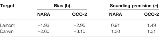
TABLE 5. Bias ($b$) and sounding precision ($\sigma$) of NARA and OCO-2 real retrievals at the two validated target locations. The units for $b$ and $\sigma$ are ppm.

Define the daily standard deviation (${\sigma }_d$) as the standard deviation of retrieved X_CO2 from 10 selected satellite observation points within a day or the standard deviation of coincident TCCON measurements within a day. Because X_CO2 can be assumed to be constant spatially and temporally during a target maneuver, the daily standard deviation is considered an artifact and can be used to discern biases caused by the algorithm’s processing of parameters. Figure 8 shows the ${\sigma }_d$ of the NARA retrieved X_CO2 and comparisons with ${\sigma }_d$ of the OCO-2 retrieved X_CO2 of the same observation points and ${\sigma }_d$ of the coincident TCCON measurements at the Lamont and Darwin locations. Whether over land or ocean, ${\sigma }_d$ of the two satellite retrievals were larger than that of coincident TCCON measurements. Sometimes ${\sigma }_d$ of satellite retrievals can be particularly large, such as ${\sigma }_d$ on September 4, 2015, at the Lamont location or ${\sigma }_d$ on March 19, 2015, at the Darwin location, which greatly exceeded ground-based values. Although retrievals of 10 randomly selected satellite observation points cannot fully represent the target-mode retrieval, the outcome indicated to a certain extent that ground-based measurements were more robust than satellite retrievals. Comparing the two satellite retrieval results, we found that ${\sigma }_d$ of NARA retrievals were generally larger than those of OCO-2, in particular for measurements at the Darwin location over the ocean. The robustness of the NARA algorithm needs to be improved further, in particular over the ocean, which may be achieved by optimizing the ensemble generation method or imposing more constraints on the parameters of the state vector in the process of minimizing the cost function.

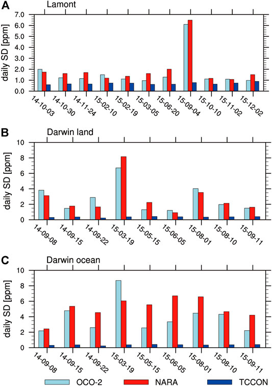
FIGURE 8. Daily standard deviation (σd) of the NARA retrieved X_CO2 and comparisons with σd of the OCO-2 retrieved X_CO2 for the same observation points and σd of the coincident TCCON data at (A) the Lamont location, (B) the Darwin location over land, and (C) the Darwin location over the ocean.

For the further contrast between different optimization methods, the medians and standard deviations of retrievals from 4DVar, NARA, OCO-2, and TCCON at the Lamont station on November 24, 2014 were compared. Without bias correction, the medians of X_CO2 from 4DVar, NARA, OCO-2, and TCCON were 403.28, 397.25, 396.19, and 398.26 ppm, respectively. The corresponding standard deviations were 8.85, 1.70, 1.15, and 0.65 ppm, respectively. The 4DVar retrieved X_CO2 was much higher than TCCON estimate, and the standard deviation was also bigger than other methods. The NARA median X_CO2 was closest to the TCCON median, and OCO-2 retrievals had the smallest standard deviation. We additionally compared the computational time consumed by each method. The retrieval time of one iteration (excluding forward simulation) from the NARA algorithm was about 0.2–0.3 s. The retrieval time of one iteration for the 4DVar method varied under different circumstances, but most exceeded 1 s. The retrieval time of OCO-2 was close to the 4DVar method.

Figure 9 shows the variation over time in NARA retrieved X_CO2 and coincident TCCON measurements at the Lamont and Darwin locations. As can be seen from the results for the Lamont location, the NARA retrievals captured well the seasonal variation in X_CO2. In addition, the retrieval results improved greatly after bias correction. After bias correction, the bias ($b$) was −0.15 ppm, and the sounding precision ($\sigma$) was 0.76 ppm. The seasonal variation in X_CO2 was much smaller in the Southern Hemisphere than in the Northern Hemisphere, and the observation data distribution for the Darwin location was inhomogeneous; therefore, the retrievals at the Darwin location did not show obvious seasonal variation, but X_CO2 increased steadily over time. The bias correction was very effective for observations over land at the Darwin location; however, it was not quite ideal for ocean observations. After the bias correction, the bias ($b$) was -0.17 ppm, and the sounding precision ($\sigma$) was 1.26 ppm. In this case, we used the bias correction method from OCO-2. Future work will focus on formulating a dedicated bias correction method for the NARA algorithm.

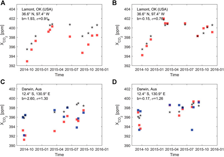
FIGURE 9. Variation over time in NARA retrieved X_CO2 over land (red squares) and ocean (blue squares) and coincident TCCON measurements (black stars) at the Lamont and Darwin locations. The NARA retrievals in (A) and (C) are before bias correction, and those in (B) and (D) are bias-corrected. In each subplot, the site location in latitude and longitude, bias (B) and sounding precision (σ) are presented. The units for b and σ are ppm.

Figure 10 shows the relationship between the median of NARA target-mode retrievals and the median of coincident TCCON data. The best fit straight lines were computed in a least squares sense. Figure 10A shows the relationship prior to bias correction and had a correlation coefficient of $R^2=0.89$. Figure 10B shows the retrieval results after bias correction and had a correlation coefficient of $R^2=0.90$. Both correlation coefficients passed the significance test at the 5% level. This demonstrates that the retrieval results were credible and that bias correction was effective, although some residual biases required further investigation.

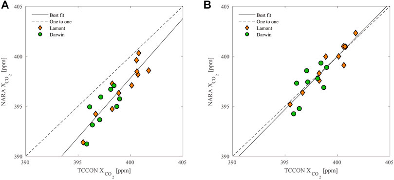
FIGURE 10. Relationships between the median of NARA target-mode retrievals and the median of coincident TCCON data. (A) Data before bias correction. (B) Data after bias correction. A one-to-one line is indicated by the dashed line, and the best fit line is indicated by the solid line.

Summary and Discussion

In this study, we developed a novel CO₂ retrieval algorithm, NARA, which used the NLS-4DVar method as the optimization method, and adopted the LIDORT radiative transfer model and necessary parameters provided by the ACOS algorithm in the forward model. The advantages of the NARA algorithm are its simplicity and efficiency given the NLS-4DVar method as its basis, as there is no need to calculate the weighting function matrix and its transposition during the retrieval process. This greatly reduces computational complexity while maintaining retrieval accuracy, which is extremely important for satellite retrievals whose data volume is quite huge.

OSSEs and real-data retrievals were carefully designed to evaluate the NARA algorithm. The OSSEs showed that the NARA retrievals of both X_CO2 and the CO₂ profile were greatly improved compared to prior values and were close to the true values. In particular, the retrieved CO₂ profiles of the two sites in the Northern Hemisphere over land captured well the real situation in the lower troposphere, where CO₂ sources and sinks are located. The effect of aerosol concentrations on X_CO2 retrieval was also discussed. We performed a set of three OSSEs with different AODs, and the results indicated that the retrieved X_CO2 was more accurate with lower aerosol concentrations. Then we performed real-data retrievals using OCO-2 target-mode observations and compared the NARA retrieved X_CO2 with coincident TCCON measurements at the Lamont and Darwin locations. Before bias correction, the mean difference between the NARA retrieved X_CO2 and coincident TCCON measurements was –1.93 ppm (SD: 0.91 ppm) at the Lamont location; the mean difference was –2.60 ppm (SD: 1.30 ppm) at the Darwin location. These results were not inferior to the OCO-2 retrieval results for the corresponding observation points. We also compared the X_CO2 retrievals with the normal 4DVar method. The retrieval bias and standard deviation of 4DVar method were bigger than NARA and OCO-2 results. Besides, the computational time consumed by one iteration from NARA was the least.

At present, the NARA algorithm is demonstrated effective, but still needs further improvements. The daily standard deviations of NARA X_CO2 retrievals were relatively large, especially over the ocean. In future work, we intend to further optimize the NARA algorithm, such as improving the prior state vector and generation of the initial ensemble, to enhance its robustness. Moreover, the algorithm was tested at several TCCON stations, next it will be tested through all TCCON stations to evaluate the retrieval results of target-, nadir-, and glint-mode observations. In addition, we plan to construct and incorporate data filtering and bias correction components customized to the NARA algorithm, and make the algorithm become an operation procedure to produce mature X_CO2 products.

Data Availability Statement

The raw data supporting the conclusions of this article will be made available by the authors, without undue reservation.

Author Contributions

ZJ: Software, Validation, Formal analysis, Investigation, Data Curation, Writing-Original Draft, Visualization XT: Conceptualization, Methodology, Resources, Writing-Review and Editing, Supervision, Funding acquisition DM: Methodology, Writing-Review and Editing, Supervision HR: Software, Investigation, Writing-Review and Editing.

Funding

This work was supported by the National Key Research and Development Program of China (2016YFA0600203), the National Natural Science Foundation of China (41575100), and the Key Research Program of Frontier Sciences, Chinese Academy of Sciences (CAS) (QYZDYSSW-DQC012).

Conflict of Interest

The authors declare that the research was conducted in the absence of any commercial or financial relationships that could be construed as a potential conflict of interest.

References

Appendix A

The following mathematical derivation exhibits how the optimal state vector is obtained without calculating the weighting function matrix and its transposition.

The first-derivative matrix $J_{ac}Q\left(\mathit{\beta }\right)$ of $Q\left(\mathit{\beta }\right)$ can be computed as follows:

where $\mathbf{I}$ denote the $N\times N$ identity matrix. The Gauss-Newton iterative solution for the nonlinear least squares problem is defined by (Dennis and Schnabel 1996):

Substituting Eqs. 10, A1 into Eq. A2, we obtain

where $\Delta {\mathit{\beta }}^i={\mathit{\beta }}^i-{\mathit{\beta }}^{i-1}$. The linear system Eq. A3 can be solved using the conjugate gradient (CG) method or a preconditioned CG method. Since ${\left(\mathbf{K}{\mathbf{P}}_x\right)}^{\mathrm{T}}$ can be obtained simply by transposing $\mathbf{K}{\mathbf{P}}_x$, the transposition of weighting function matrix is nicely avoided.

We substitute ${\mathbf{P}}_y=\mathbf{K}{\mathbf{P}}_x$ and ${\mathit{\beta }}^{i-1}\approx {\left[{\left({\mathbf{P}}_y\right)}^{\mathrm{T}}\left({\mathbf{P}}_y\right)\right]}^{-1}{\left({\mathbf{P}}_y\right)}^{\mathrm{T}}\mathbf{K}\left({\mathbf{P}}_x{\mathit{\beta }}^{i-1}\right)$ into Eq. A3 and obtain:

where

and

Here $\Delta {\mathit{\beta }}^i$ can be computed explicitly by Eq. A4 and the CG iterations are thus avoided.

To further reduce the implementation complexity by abandoning the use of the weighting function matrix, we rewrite Eq. A4 into

where

and

References

Baker, D. F., Bösch, H., Doney, S. C., O'Brien, D., and Schimel, D. S. (2010). Carbon Source/sink Information provided by Column CO2 Measurements from the Orbiting Carbon Observatory. Atmos. Chem. Phys. 10 (9), 4145–4165. doi:10.5194/acp-10-4145-2010
Boesch, H., Baker, D., Connor, B., Crisp, D., and Miller, C. (2011). Global Characterization of CO2 Column Retrievals from Shortwave-Infrared Satellite Observations of the Orbiting Carbon Observatory-2 Mission. Remote Sensing. 3 (2), 270-304. doi:10.3390/rs3020270
Buchwitz, M., de Beek, R., Noël, S., Burrows, J. P., Bovensmann, H., Bremer, H., et al. (2005). Carbon Monoxide, Methane and Carbon Dioxide Columns Retrieved from SCIAMACHY by WFM-DOAS: Year 2003 Initial Data Set. Atmos. Chem. Phys. 5 (12), 3313-3329. doi:10.5194/acp-5-3313-2005
Buchwitz, M., Rozanov, V. V., and Burrows, J. P. (2000). A Near-Infrared Optimized DOAS Method for the Fast Global Retrieval of Atmospheric CH4, CO, CO2, H2O, and N2O Total Column Amounts from SCIAMACHY Envisat-1 Nadir Radiances. J. Geophys. Res. 105 (D12), 15231-15245. doi:10.1029/2000jd900191
Butz, A., Galli, A., Hasekamp, O., Landgraf, J., Tol, P., and Aben, I. (2012). TROPOMI Aboard Sentinel-5 Precursor: Prospective Performance of CH4 Retrievals for Aerosol and Cirrus Loaded Atmospheres. Remote Sensing Environ. 120, 267-276. doi:10.1016/j.rse.2011.05.030
Butz, A., Guerlet, S., Hasekamp, O., Schepers, D., Galli, A., Aben, I., et al. (2011). Toward Accurate CO2 and CH4 observations from GOSAT. Geophys. Res. Lett. 38 (14), a-n. doi:10.1029/2011gl047888
Butz, A., Hasekamp, O. P., Frankenberg, C., and Aben, I. (2009). Retrievals of Atmospheric CO2 from Simulated Space-Borne Measurements of Backscattered Near-Infrared Sunlight: Accounting for Aerosol Effects. Appl. Opt. 48 (18), 3322-3336. doi:10.1364/ao.48.003322
Chédin, A., Serrar, S., Scott, N. A., Crevoisier, C., and Armante, R. (2003). First Global Measurement of Midtropospheric CO2 from NOAA Polar Satellites: Tropical Zone. J. Geophys. Res. 108 (D18), 4581. doi:10.1029/2003jd003439
Cogan, A. J., Boesch, H., Parker, R. J., Feng, L., Palmer, P. I., Blavier, J.-F. L., et al. (2012). Atmospheric Carbon Dioxide Retrieved from the Greenhouse Gases Observing SATellite (GOSAT): Comparison with Ground-Based TCCON Observations and GEOS-Chem Model Calculations. J. Geophys. Res. 117 (21), a-n. doi:10.1029/2012jd018087
Connor, B. J., Boesch, H., Toon, G., Sen, B., Miller, C., and Crisp, D. (2008). Orbiting Carbon Observatory: Inverse Method and Prospective Error Analysis. J. Geophys. Res. 113 (D5), a-n. doi:10.1029/2006jd008336
Cox, P. M., Betts, R. A., Jones, C. D., Spall, S. A., and Totterdell, I. J. (2000). Acceleration of Global Warming Due to Carbon-Cycle Feedbacks in a Coupled Climate Model. Nature. 408 (6809), 184-187. doi:10.1038/35041539
Crevoisier, C., Chédin, A., Matsueda, H., Machida, T., Armante, R., and Scott, N. A. (2009). First Year of Upper Tropospheric Integrated Content of CO2 from IASI Hyperspectral Infrared Observations. Atmos. Chem. Phys. 9 (14), 4797-4810. doi:10.5194/acp-9-4797-2009
Crisp, D., Atlas, R. M., Breon, F.-M., Brown, L. R., Burrows, J. P., Ciais, P., et al. (2004). The Orbiting Carbon Observatory (OCO) mission. Adv. Space Res. 34 (4), 700-709. doi:10.1016/j.asr.2003.08.062
Crisp, D., Fisher, B. M., O'Dell, C., Frankenberg, C., Basilio, R., Bösch, H., et al. (2012). The ACOS CO2 Retrieval Algorithm - Part II: Global XCO2 Data Characterization. Atmos. Meas. Tech. 5 (4), 687-707. doi:10.5194/amt-5-687-2012
Crisp, D., Pollock, H. R., Rosenberg, R., Chapsky, L., Lee, R. A. M., Oyafuso, F. A., et al. (2017). The On-Orbit Performance of the Orbiting Carbon Observatory-2 (OCO-2) Instrument and its Radiometrically Calibrated Products. Atmos. Meas. Tech. 10 (1), 59–81. doi:10.5194/amt-10-59-2017
Dennis, J. E., and Schnabel, R. B. (1996). Numerical Methods for Unconstrained Optimization and Nonlinear Equations. Philadelphia, PA, USA: Society for Industrial and Applied Mathematics. doi:10.1137/1.9781611971200
Dilling, L., Doney, S. C., Edmonds, J., Gurney, K. R., Harriss, R., Schimel, D., et al. (2003). Therole Ofcarboncycleobservations Andknowledge Incarbonmanagement. Annu. Rev. Environ. Resour. 28, 521-558. doi:10.1146/annurev.energy.28.011503.163443
Eldering, A., Taylor, T. E., O'Dell, C. W., and Pavlick, R. (2019). The OCO-3 mission: Measurement Objectives and Expected Performance Based on 1 Year of Simulated Data. Atmos. Meas. Tech. 12 (4), 2341–2370. doi:10.5194/amt-12-2341-2019
Evensen, G. (2009). Data Assimilation: The Ensemble Kalman Filter. Berlin Heidelberg: Springer-Verlag. doi:10.1007/978-3-642-03711-5
Griffith, D. W. T., Deutscher, N. M., Velazco, V. A., Wennberg, P. O., Yavin, Y., Keppel-Aleks, G., et al. (2014). TCCON Data from Darwin (AU). Anmeyondo, South Korea, Release GGG2014R0, TCCON data archive: CaltechDATA
Guerlet, S., Butz, A., Schepers, D., Basu, S., Hasekamp, O. P., Kuze, A., et al. (2013). Impact of Aerosol and Thin Cirrus on Retrieving and Validating XCO2 from GOSAT Shortwave Infrared Measurements. J. Geophys. Res. Atmos. 118 (10), 4887-4905. doi:10.1002/jgrd.50332
Han, R., and Tian, X. (2019). A Dual-Pass Carbon Cycle Data Assimilation System to Estimate Surface CO2 Fluxes and 3D Atmospheric CO2 Concentrations from Spaceborne Measurements of Atmospheric CO2. Geoscientific Model. Develop. Discussion Rev. doi:10.5194/gmd-2019-54
Hasekamp, O. P., and Butz, A. (2008). Efficient Calculation of Intensity and Polarization Spectra in Vertically Inhomogeneous Scattering and Absorbing Atmospheres. J. Geophys. Res. 113 (D20), D20309. doi:10.1029/2008JD010379
Hoinka, K. P. (1998). Statistics of the Global Tropopause Pressure. Mon. Wea. Rev. 126, 3303-3325. doi:10.1175/1520-0493(1998)126<3303:SOTGTP>2.0.CO;2
Hönninger, G., von Friedeburg, C., and Platt, U. (2004). Multi axis Differential Optical Absorption Spectroscopy (MAX-DOAS). Atmos. Chem. Phys. 4, 231-254. doi:10.5194/acp-4-231-2004
Jiang, X., and Yung, Y. L. (2019). Global Patterns of Carbon Dioxide Variability from Satellite Observations. Annu. Rev. Earth Planet. Sci. 47, 225-245. doi:10.1146/annurev-earth-053018-060447
Kulawik, S. S., Jones, D. B. A., Nassar, R., Irion, F. W., Worden, J. R., Bowman, K. W., et al. (2010). Characterization of Tropospheric Emission Spectrometer (TES) CO2 for Carbon Cycle Science. Atmos. Chem. Phys. 10 (12), 5601-5623. doi:10.5194/acp-10-5601-2010
Le Quéré, C., Andrew, R. M., Canadell, J. G., Sitch, S., Ivar Korsbakken, J., Peters, G. P., et al. (2016). Global Carbon Budget 2016. Earth Syst. Sci. Data 8 (2), 605-649. doi:10.5194/essd-8-605-2016
Miller, C. E., Crisp, D., DeCola, P. L., Olsen, S. C., Randerson, J. T., Michalak, A. M., et al. (2007). Precision Requirements for Space-Based Data. J. Geophys. Res. 112 (D10), D10314. doi:10.1029/2006jd007659
Nakajima, M., Kuze, A., and Suto, H. (2012). The Current Status of GOSAT and the Concept of GOSAT-2. In Sensors, Systems, and Next-Generation Satellites XVI. Edinburgh, United Kingdom: Society of Photo-Optical Instrumentation Engineers, 853306.
O'Dell, C. W., Connor, B., Bösch, H., O'Brien, D., Frankenberg, C., Castano, R., et al. (2012). The ACOS CO2 Retrieval Algorithm - Part 1: Description and Validation against Synthetic Observations. Atmos. Meas. Tech. 5 (1), 99-121. doi:10.5194/amt-5-99-2012
O'Dell, C. W., Eldering, A., Wennberg, P. O., Crisp, D., Gunson, M. R., Fisher, B., et al. (2018). Improved Retrievals of Carbon Dioxide from Orbiting Carbon Observatory-2 with the Version 8 ACOS Algorithm. Atmos. Meas. Tech. 11 (12), 6539-6576. doi:10.5194/amt-11-6539-2018
Rayner, P. J., and O'Brien, D. M. (2001). The Utility of Remotely Sensed CO2 concentration Data in Surface Source Inversions. Geophys. Res. Lett. 28 (1), 175-178. doi:10.1029/2000gl011912
Reuter, M., Bösch, H., Bovensmann, H., Bril, A., Buchwitz, M., Butz, A., et al. (2013). A Joint Effort to Deliver Satellite Retrieved Atmospheric CO2 Concentrations for Surface Flux Inversions: the Ensemble Median Algorithm EMMA. Atmos. Chem. Phys. 13 (4), 1771–1780. doi:10.5194/acp-13-1771-2013
Reuter, M., Bovensmann, H., Buchwitz, M., Burrows, J. P., Connor, B. J., Deutscher, N. M., et al. (2011). Retrieval of Atmospheric CO2 with Enhanced Accuracy and Precision from SCIAMACHY: Validation with FTS Measurements and Comparison with Model Results. J. Geophys. Res. 116 (D4), D04301. doi:10.1029/2010jd015047
Reuter, M., Buchwitz, M., Schneising, O., Heymann, J., Bovensmann, H., and Burrows, J. P. (2010). A Method for Improved SCIAMACHY CO2 Retrieval in the Presence of Optically Thin Clouds. Atmos. Meas. Tech. 3 (1), 209-232. doi:10.5194/amt-3-209-2010
Schneising, O., Bergamaschi, P., Bovensmann, H., Buchwitz, M., Burrows, J. P., Deutscher, N. M., et al. (2012). Atmospheric Greenhouse Gases Retrieved from SCIAMACHY: Comparison to Ground-Based FTS Measurements and Model Results. Atmos. Chem. Phys. 12 (3), 1527-1540. doi:10.5194/acp-12-1527-2012
Spurr, R. J. D., Kurosu, T. P., and Chance, K. V. (2001). A Linearized Discrete Ordinate Radiative Transfer Model for Atmospheric Remote-Sensing Retrieval. J. Quantitative Spectrosc. Radiative Transfer 68 (6), 689-735. doi:10.1016/S0022-4073(00)00055-8
Spurr, R., and Natraj, V. (2011). A Linearized Two-Stream Radiative Transfer Code for Fast Approximation of Multiple-Scatter fields. J. Quantitative Spectrosc. Radiative Transfer. 112 (16), 2630–2637. doi:10.1016/j.jqsrt.2011.06.014
Taylor, T. E., O'Dell, C. W., Frankenberg, C., Partain, P. T., Cronk, H. Q., Savtchenko, A., et al. (2016). Orbiting Carbon Observatory-2 (OCO2) Cloud Screening Algorithms: Validation against Collocated MODIS and CALIOP Data. Atmos. Meas. Tech. 9 (3), 973-989. doi:10.5194/amt-9-973-2016
Tian, X., Xie, Z., Liu, Y., Cai, Z., Fu, Y., Zhang, H., et al. (2014a). A Joint Data Assimilation System (Tan-Tracker) to Simultaneously Estimate Surface CO2 Fluxes and 3-D Atmospheric CO2 Concentrations from Observations. Atmos. Chem. Phys. 14 (23), 13281–13293. doi:10.5194/acp-14-13281-2014
Tian, X., Xie, Z., Cai, Z., Liu, Y., Fu, Y., and Zhang, H. (2014b). The Chinese Carbon Cycle Data-Assimilation System (Tan-Tracker). Chinese Sci. Bull. 59 (14), 1541–1546. doi:10.1007/s11434-014-0238-1
Tian, X., and Feng, X. (2015). A Non-linear Least Squares Enhanced POD-4DVar Algorithm for Data Assimilation. Tellus A: Dynamic Meteorology and Oceanography. 67 (1), 25340. doi:10.3402/tellusa.v67.25340
Tian, X., Zhang, H., Feng, X., and Xie, Y. (2018). Nonlinear Least Squares En4DVar to 4DEnVar Methods for Data Assimilation: Formulation, Analysis, and Preliminary Evaluation. Monthly Weather Rev. 146 (1), 77-93. doi:10.1175/mwr-d-17-0050.1
Wennberg, P. O., Wunch, D., Roehl, C. M., Blavier, J.-F., Toon, G. C., and Allen, N. T. (2016). TCCON Data from Lamont (US). (GGG2014R1, TCCON data archive: CaltechDATA)
Wu, L., Hasekamp, O., Hu, H., Landgraf, J., Butz, A., aan de Brugh, J., et al. (2018). Carbon Dioxide Retrieval from OCO-2 Satellite Observations Using the RemoTeC Algorithm and Validation with TCCON Measurements. Atmos. Meas. Tech. 11 (5), 3111-3130. doi:10.5194/amt-11-3111-2018
Wunch, D., Toon, G. C., Blavier, J. F. L., Washenfelder, R. A., Notholt, J., Connor, B. J., et al. (2011). The Total Carbon Column Observing Network. Phil. Trans. R. Soc. A. 369, 2087-2112. doi:10.1098/rsta.2010.0240
Wunch, D., Wennberg, P. O., Osterman, G., Fisher, B., Naylor, B., Roehl, C. M., et al. (2017). Comparisons of the Orbiting Carbon Observatory-2 (OCO-2) XCO2 Measurements with TCCON. Atmos. Meas. Tech. 10 (6), 2209-2238. doi:10.5194/amt-10-2209-2017
Yang, D., Liu, Y., Cai, Z., Chen, X., Yao, L., and Lu, D. (2018). First Global Carbon Dioxide Maps Produced from TanSat Measurements. Adv. Atmos. Sci. 35 (6), 621-623. doi:10.1007/s00376-018-7312-6
Yokota, T., Yoshida, Y., Eguchi, N., Ota, Y., Tanaka, T., Watanabe, H., et al. (2009). Global Concentrations of CO2 and CH2 Retrieved from GOSAT: First Preliminary Results. Sola. 5 (1), 160-163. doi:10.2151/sola.2009‒04110.2151/sola.2009-041
Yoshida, Y., Ota, Y., Eguchi, N., Kikuchi, N., Nobuta, K., Tran, H., et al. (2011). Retrieval Algorithm for CO2 and CH2 Column Abundances from Short-Wavelength Infrared Spectral Observations by the Greenhouse Gases Observing Satellite. Atmos. Meas. Tech. 4 (4), 717-734. doi:10.5194/amt-4-717-2011
Yue, T., Zhang, L., Zhao, M., Wang, Y., and Wilson, J. (2016). Space- and Ground-Based CO2 Measurements: A Review. Sci. China Earth Sci. 59 (11), 2089-2097. doi:10.1007/s11430-015-0239-7
Zhang, H. (2019). Improvement and Application of Nonlinear Least Squares Ensemble Four-Dimensional Variational Assimilation Method. Beijing, China: Institute of Atmospheric Physics, Chinese Academy of Sciences.