
Utilizing TVDI and NDWI to Classify Severity of Agricultural Drought in Chuping, Malaysia

 , , ,
, , ,  ,
,  and
and 
Abstract
:1. Introduction

| Agricultural Drought Indices | Formula | Advantages | Limitation |
|---|---|---|---|
| NDVI | [28] |
| |
| VCI | [30] noting that NDVIi represents the continuous mean NDVI of a certain period i e.g., a month, NDVImax represents the maximum NDVI and NDVImin represents the minimum NDVI. | ||
| TCI | [30] where the smoothed weekly brightness temperature, multi-year maximum and multi-year minimum, respectively, at each grid cell are BTj, BTmax and BTmin. |
|
|
| VHI | [37]
is the coefficient defining the contribution of the two indices at 0.5. A VHI value of less than 40 indicates the presence of vegetation stress, while a value of greater than 60 indicates that the vegetation is in good condition. |
| |
| SVI | VI whereby both either NDVI or EVI can be utilized [41]. Adding on is the z-value for pixel i during week j for year k. |
|
|
| NDWI | [22] |
| |
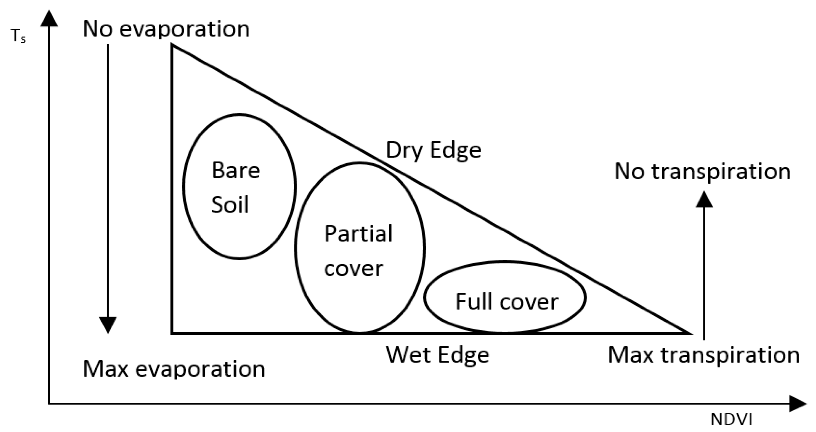
| TVDI | [46] |
2. Materials and Methods
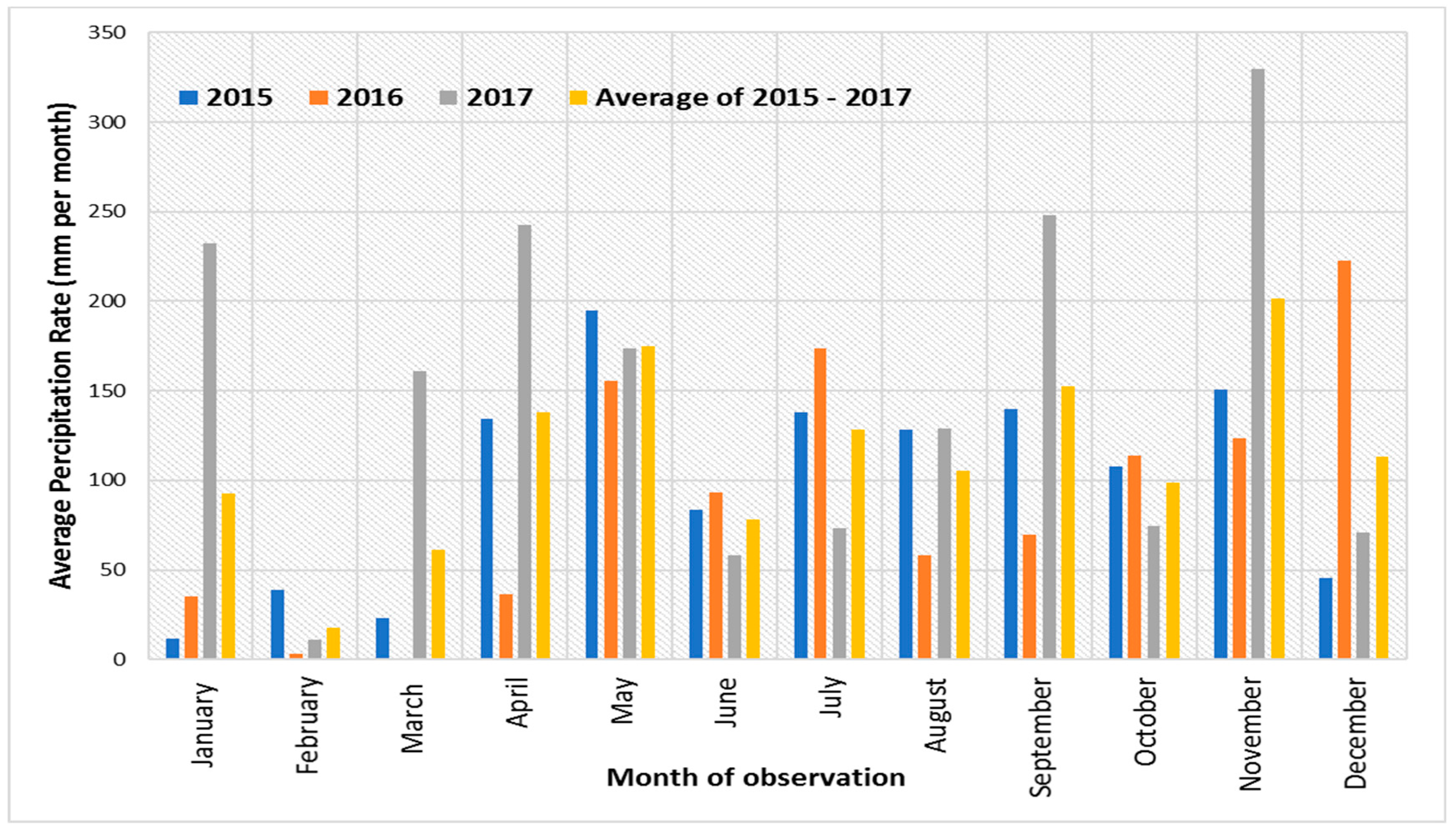
2.1. Meteorology Data
2.2. Landsat Image Processing
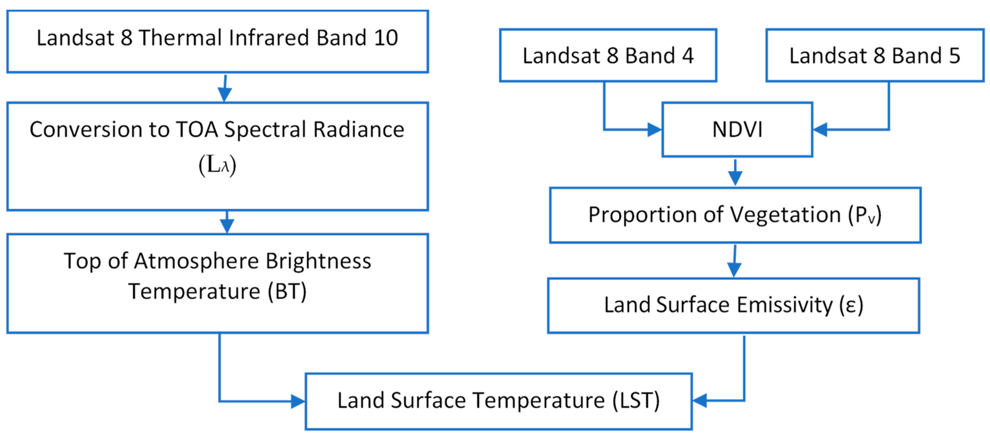
2.3. Steps in Derivation of LST
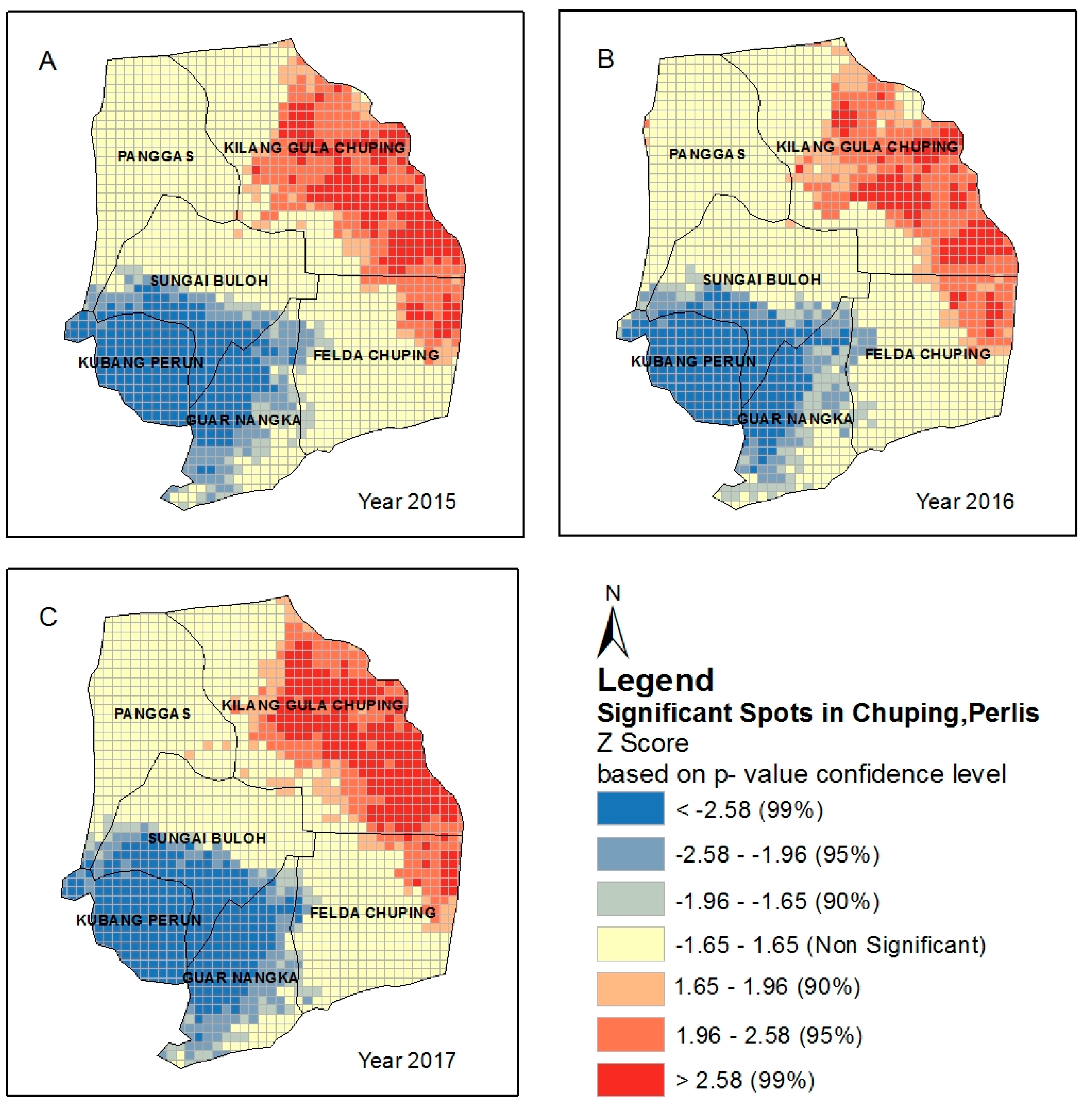
2.4. Statistical Analysis and Derivation of Global Moran’s Index
3. Results and Discussions
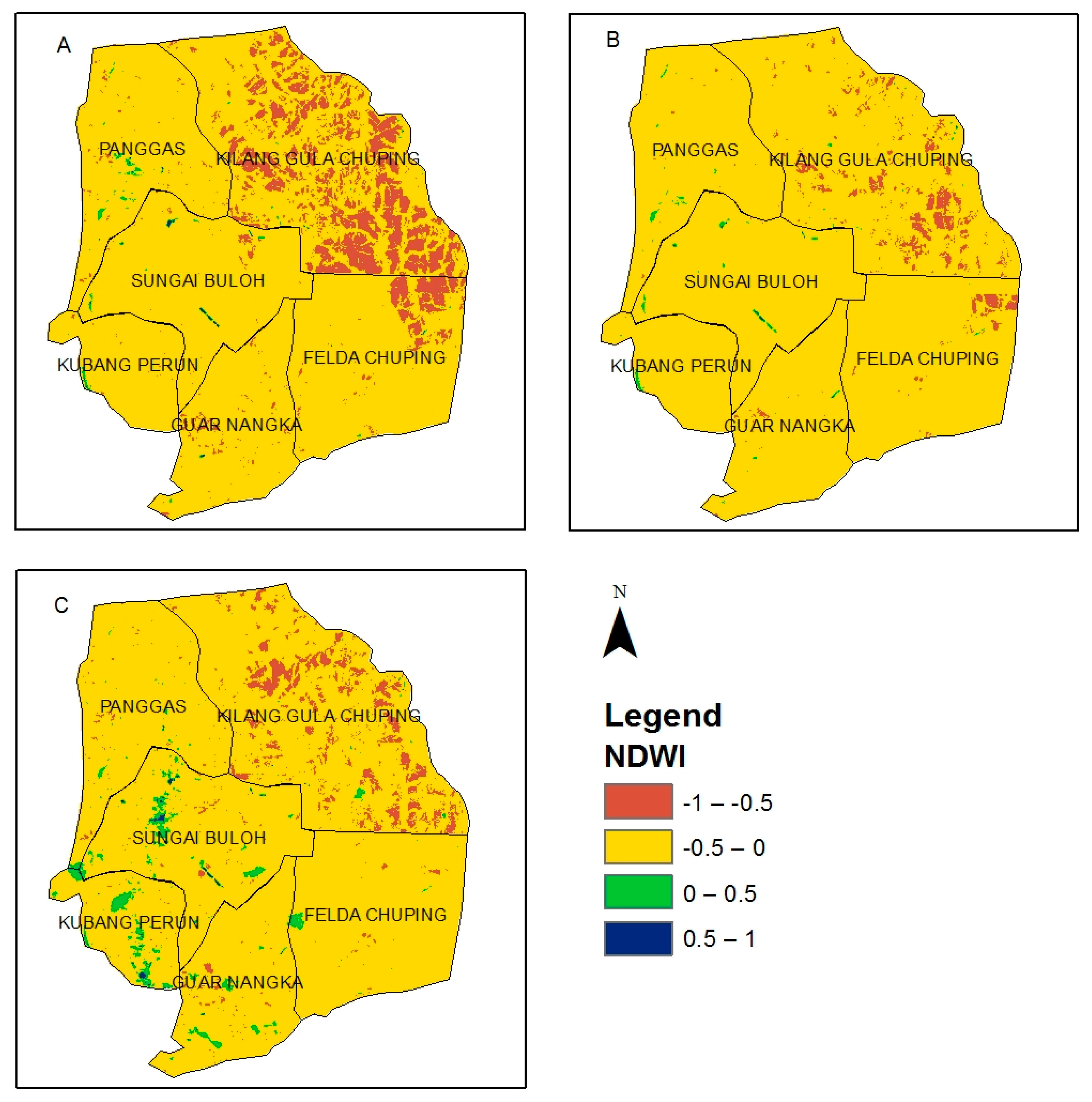
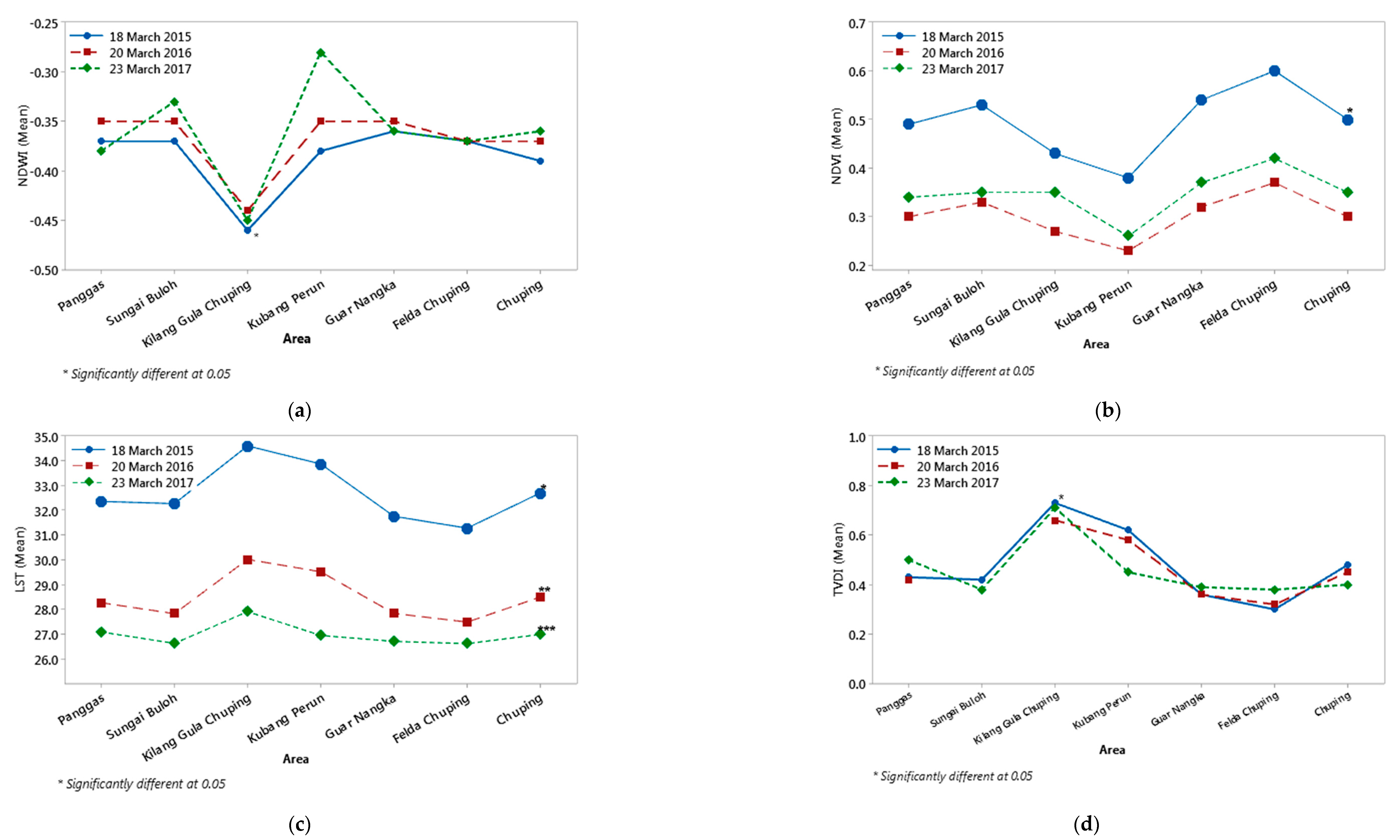
3.1. NDWI Derivation
3.2. NDVI Derivation
3.3. TVDI Derivation
3.4. Correlation of TVDI and NDWI
4. Conclusions
Author Contributions
Funding
Institutional Review Board Statement
Informed Consent Statement
Data Availability Statement
Acknowledgments
Conflicts of Interest
References
- Moneo, M.; Iglesias, A. España Food and Climate; Universidad Politécnica de Madrid: Madrid, Spain, 2004. [Google Scholar]
- Dai, A. Increasing drought under global warming in observations and models. Nat. Clim. Chang. 2012, 3, 52–58. [Google Scholar] [CrossRef]
- Bhandari, G.; Panthi, B.B. Analysis of Agricultural Drought and its Effects on Productivity at Different District of Nepal. J. Inst. Sci. Technol. 2015, 19, 106–110. [Google Scholar] [CrossRef] [Green Version]
- Anjum, S.A.; Ashraf, U.; Zohaib, A.; Tanveer, M.; Naeem, M.; Ali, I.; Tabassum, T.; Nazir, U. Growth and developmental responses of crop plants under drought stress: A review. Zemdirb. Agric. 2017, 104, 267–276. [Google Scholar] [CrossRef]
- Fang, Y.; Xiong, L. General mechanisms of drought response and their application in drought resistance improvement in plants. Cell. Mol. Life Sci. 2015, 72, 673–689. [Google Scholar] [CrossRef] [PubMed]
- Legros, S.; Mialet-Serra, I.; Clement-Vidal, A.; Caliman, J.-P.; Siregar, F.; Fabre, D.; Dingkuhn, M. Role of transitory carbon reserves during adjustment to climate variability and source-sink imbalances in oil palm (Elaeis guineensis). Tree Physiol. 2009, 29, 1199–1211. [Google Scholar] [CrossRef] [Green Version]
- Tadesse, A.; Anteneh, A.M. Drought Tolerance Mechanisms in Field Crops. World J. Biol. Med. Sci. 2016, 3, 15–19. [Google Scholar]
- Putra, E.T.; Purwanto, B.H. Physiological Responses of Oil Palm Seedlings to the Drought Stress Using Boron and Silicon Applications. J. Agron. 2015, 14, 49–61. [Google Scholar] [CrossRef] [Green Version]
- Noor, M.R.M.; Harun, M.H. Water Deficit and Irrigation in Oil Palm: A Review of Recent Studies and Findings. Oil Palm Bull. 2004, 49, 1–6. [Google Scholar]
- Caliman’, J.P.; Southworth, A.; Caliman, J.P.; Southworth, A. Effect of Drought and Haze on the Performance of Oil Palm. 1998. Available online: https://agritrop.cirad.fr/401034/ (accessed on 28 April 2021).
- Corley, R.H.V.; Rao, V.; Palat, T.; Praiwan, T. Breeding for drought tolerance in oil palm. J. Oil Palm Res. 2018, 30, 26–35. [Google Scholar]
- Ji, K.; Wang, Y.; Sun, W.; Lou, Q.; Mei, H.; Shen, S.; Chen, H. Drought-responsive mechanisms in rice genotypes with contrasting drought tolerance during reproductive stage. J. Plant Physiol. 2012, 169, 336–344. [Google Scholar] [CrossRef] [PubMed]
- Zhang, J.; Zhang, S.; Cheng, M.; Jiang, H.; Zhang, X.; Peng, C.; Lu, X.; Zhang, M.; Jin, J. Effect of Drought on Agronomic Traits of Rice and Wheat: A Meta-Analysis. Int. J. Environ. Res. Public Health 2018, 15, 839. [Google Scholar] [CrossRef] [Green Version]
- Khaled, K.A.; El-Arabi, N.I.; Sabry, N.M.; El-Sherbiny, S. Sugarcane Genotypes Assessment Under Drought Condition Using Amplified Fragment Length Polymorphism. Biotechnology 2018, 17, 120–127. [Google Scholar] [CrossRef] [Green Version]
- Bartels, D.; Sunkar, R. Drought and Salt Tolerance in Plants. Crit. Rev. Plant Sci. 2005, 24, 23–58. [Google Scholar] [CrossRef]
- Wahid, A.; Close, T.J. Expression of dehydrins under heat stress and their relationship with water relations of sugarcane leaves. Biol. Plant. 2007, 51, 104–109. [Google Scholar] [CrossRef]
- Ebrahim, M.K.; Zingsheim, O.; El-Shourbagy, M.N.; Moore, P.H.; Komor, E. Growth and sugar storage in sugarcane grown at temperatures below and above optimum. J. Plant Physiol. 1998, 153, 593–602. [Google Scholar] [CrossRef]
- Xue, J.; Su, B. Significant Remote Sensing Vegetation Indices: A Review of Developments and Applications. J. Sens. 2017, 2017, 1–17. [Google Scholar] [CrossRef] [Green Version]
- Gandhi, G.M.; Parthiban, S.; Thummalu, N.; Christy, A. Ndvi: Vegetation Change Detection Using Remote Sensing and Gis—A Case Study of Vellore District. Procedia Comput. Sci. 2015, 57, 1199–1210. [Google Scholar] [CrossRef] [Green Version]
- Seelig, H.D.; Hoehn, A.; Stodieck, L.S.; Klaus, D.M.; Emery, W.J. The assessment of leaf water content using leaf reflectance ratios in the visible, near-, and short-wave-infrared. Int. J. Remote Sens. 2008, 29, 3701–3713. [Google Scholar] [CrossRef]
- AghaKouchak, A.; Farahmand, A.M.; Melton, F.S.; Teixeira, J.P.; Anderson, M.C.; Wardlow, B.D.; Hain, C.R. Remote sensing of drought: Progress, challenges and opportunities. Rev. Geophys. 2015, 53, 452–480. [Google Scholar] [CrossRef] [Green Version]
- Gao, B.-C. NDWI—A normalized difference water index for remote sensing of vegetation liquid water from space. Remote Sens. Environ. 1995, 58, 257–266. [Google Scholar] [CrossRef]
- Zhang, C.; Pattey, E.; Liu, J.; Cai, H.; Shang, J.; Dong, T. Retrieving Leaf and Canopy Water Content of Winter Wheat Using Vegetation Water Indices. IEEE J. Sel. Top. Appl. Earth Obs. Remote Sens. 2017, 11, 112–126. [Google Scholar] [CrossRef]
- Ji, L.; Zhang, L.; Wylie, B. Analysis of Dynamic Thresholds for the Normalized Difference Water Index. Photogramm. Eng. Remote Sens. 2009, 75, 1307–1317. [Google Scholar] [CrossRef]
- Dangwal, N. Detection of Crop Water Stress and Its Impact on Productivity of Cropland Ecosystem. 2014. Available online: https://www.iirs.gov.in/content/detection-crop-water-stress-and-its-impact-productivity-cropland-ecosystem (accessed on 30 March 2021).
- Liang, L.; Zhao, S.-H.; Qin, Z.-H.; He, K.-X.; Chen, C.; Luo, Y.-X.; Zhou, X.-D. Drought Change Trend Using MODIS TVDI and Its Relationship with Climate Factors in China from 2001 to 2010. J. Integr. Agric. 2014, 13, 1501–1508. [Google Scholar] [CrossRef]
- Meng, L.; Li, J.; Chen, Z.; Xi, W.; Chen, D.; Duan, H. The Calculation of TVDI Based on the Composite of Pixel and Drought Analysis. Int. Arch. Photogramm. Remote Sens. Spat. Inf. Sci. 2008, 38, 519–524. [Google Scholar]
- Tucker, C.J. Red and photographic infrared linear combinations for monitoring vegetation. Remote Sens. Environ. 1979, 8, 127–150. [Google Scholar] [CrossRef] [Green Version]
- Avitabile, V.; Baccini, A.; Friedl, M.A.; Schmullius, C. Capabilities and limitations of Landsat and land cover data for aboveground woody biomass estimation of Uganda. Remote Sens. Environ. 2012, 117, 366–380. [Google Scholar] [CrossRef]
- Kogan, F. Application of vegetation index and brightness temperature for drought detection. Adv. Space Res. 1995, 15, 91–100. [Google Scholar] [CrossRef]
- Liu, W.T.; Kogan, F.N. Monitoring regional drought using the Vegetation Condition Index. Int. J. Remote Sens. 1996, 17, 2761–2782. [Google Scholar] [CrossRef]
- Han, Y.; Li, Z.; Huang, C.; Zhou, Y.; Zong, S.; Hao, T.; Niu, H.; Yao, H. Monitoring Droughts in the Greater Changbai Mountains Using Multiple Remote Sensing-Based Drought Indices. Remote Sens. 2020, 12, 530. [Google Scholar] [CrossRef] [Green Version]
- Bayarjargal, Y.; Karnieli, A.; Bayasgalan, M.; Khudulmur, S.; Gandush, C.; Tucker, C. A comparative study of NOAA–AVHRR derived drought indices using change vector analysis. Remote Sens. Environ. 2006, 105, 9–22. [Google Scholar] [CrossRef]
- Sholihah, R.I.; Trisasongko, B.H.; Shiddiq, D.; Iman, L.O.S.; Kusdaryanto, S.; Manijo; Panuju, D.R. Identification of Agricultural Drought Extent Based on Vegetation Health Indices of Landsat Data: Case of Subang and Karawang, Indonesia. Procedia Environ. Sci. 2016, 33, 14–20. [Google Scholar] [CrossRef] [Green Version]
- Padhee, S.K. Agricultural Drought Assessment under Irrigated and Rainfed Conditions. Ph.D. Thesis, Andhra University, Andhra Pradesh, India, 2013. [Google Scholar]
- Singh, R.P.; Roy, S.; Kogan, F. Vegetation and temperature condition indices from NOAA AVHRR data for drought monitoring over India. Int. J. Remote Sens. 2003, 24, 4393–4402. [Google Scholar] [CrossRef]
- Kogan, F. World droughts in the new millennium from AVHRR-based vegetation health indices. Eos 2002, 83, 557–563. [Google Scholar] [CrossRef]
- Yu, H.; Li, L.; Liu, Y.; Li, J. Construction of Comprehensive Drought Monitoring Model in Jing-Jin-Ji Region Based on Multisource Remote Sensing Data. Water 2019, 11, 1077. [Google Scholar] [CrossRef] [Green Version]
- Bento, V.A.; Trigo, I.F.; Gouveia, C.M.; DaCamara, C.C. Contribution of Land Surface Temperature (TCI) to Vegetation Health Index: A Comparative Study Using Clear Sky and All-Weather Climate Data Records. Remote Sens. 2018, 10, 1324. [Google Scholar] [CrossRef] [Green Version]
- Wgnn, J.; Vmi, C. Investigate the Sensitivity of the Satellite-Based Agricultural Drought Indices to Monitor the Drought Condition of Paddy and Introduction to Enhanced Multi-Temporal Drought Indices. J. Remote Sens. GIS 2020, 9, 271. [Google Scholar]
- Peters, A.J.; Walter-Shea, E.A.; Ji, L.; Viña, A.; Hayes, M.; Svoboda, M.D. Drought monitoring with NDVI-based Standardized Vegetation Index. Photogramm. Eng. Remote Sens. 2002, 68, 71–75. [Google Scholar]
- Uttaruk, Y.; Laosuwan, T. Drought Analysis Using Satellite-Based Data and Spectral Index in Upper Northeastern Thailand. Pol. J. Environ. Stud. 2019, 28, 4447–4454. [Google Scholar] [CrossRef]
- Shukla, V. Modelling Spatio-Temporal Pattern of Drought Using Three-Dimensional Markov Random Field. 2007. Available online: https://www.iirs.gov.in/iirs/sites/default/files/StudentThesis/virat_thesis.pdf (accessed on 30 May 2021).
- Campos, J.C.; Sillero, N.; Brito, J. Normalized difference water indexes have dissimilar performances in detecting seasonal and permanent water in the Sahara–Sahel transition zone. J. Hydrol. 2012, 464–465, 438–446. [Google Scholar] [CrossRef]
- Herndon, K.; Muench, R.; Cherrington, E.; Griffin, R. An Assessment of Surface Water Detection Methods for Water Resource Management in the Nigerien Sahel. Sensors 2020, 20, 431. [Google Scholar] [CrossRef] [Green Version]
- Sandholt, I.; Rasmussen, K.; Andersen, J. A simple interpretation of the surface temperature/vegetation index space for assessment of surface moisture status. Remote Sens. Environ. 2002, 79, 213–224. [Google Scholar] [CrossRef]
- Przeździecki, K.; Zawadzki, J.; Miatkowski, Z. Use of the temperature–vegetation dryness index for remote sensing grassland moisture conditions in the vicinity of a lignite open-cast mine. Environ. Earth Sci. 2018, 77, 623. [Google Scholar] [CrossRef]
- Rahimzadeh-Bajgiran, P.; Omasa, K.; Shimizu, Y. Comparative evaluation of the Vegetation Dryness Index (VDI), the Temperature Vegetation Dryness Index (TVDI) and the improved TVDI (iTVDI) for water stress detection in semi-arid regions of Iran. Isprs J. Photogramm. Remote Sens. 2012, 68, 1–12. [Google Scholar] [CrossRef]
- Chen, S.; Wen, Z.; Jiang, H.; Zhao, Q.; Zhang, X.; Chen, Y. Temperature Vegetation Dryness Index Estimation of Soil Moisture under Different Tree Species. Sustainability 2015, 7, 11401–11417. [Google Scholar] [CrossRef] [Green Version]
- Faassen, K.; Nolet, C.; Contreras, S. Determining the Dryness Index and Evaporative Fraction for Satellite and Drone Images Internship Report. 2020. Available online: https://www.futurewater.nl/wp-content/uploads/2020/12/KimFaassen_InternshipReport_final.pdf (accessed on 1 June 2021).
- Hard, S. A Low-Cost Normalized Difference Vegetation Index (NDVI) A Low-Cost Normalized Difference Vegetation Index (NDVI) Payload for Cubesats and Unmanned Aerial Vehicles (UAVs) Payload for Cubesats and Unmanned Aerial Vehicles (UAVs). 2018. Available online: https://researchrepository.wvu.edu/etd/5761/ (accessed on 2 April 2021).
- Observatory, E.D. NDWI (Normalized Difference Water Index). Prod. Fact Sheet 2011, 5, 6–7. [Google Scholar]
- Jackson, T. Vegetation water content mapping using Landsat data derived normalized difference water index for corn and soybeans. Remote Sens. Environ. 2004, 92, 475–482. [Google Scholar] [CrossRef]
- Sánchez-Ruiz, S.; Piles, M.; Sánchez, N.; Martínez-Fernández, J.; Vall-llossera, M.; Camps, A. Combining SMOS with visible and near/shortwave/thermal infrared satellite data for high resolution soil moisture estimates. J. Hydrol. 2014, 516, 273–283. [Google Scholar] [CrossRef]
- U.S. Geological Survey. Landsat 8 Data Users Handbook. Nasa 2016, 8, 97. [Google Scholar]
- Carlson, T.N.; Riziley, D.A. On the Relation between NDVI, Fractional Vegetation Cover, and Leaf Area Index. Remote Sens. Environ. 1997, 62, 241–252. [Google Scholar] [CrossRef]
- Sobrino, J.A.; Jiménez-Muñoz, J.C.; Paolini, L. Land surface temperature retrieval from LANDSAT TM 5. Remote Sens. Environ. 2004, 90, 434–440. [Google Scholar] [CrossRef]
- Guo, J.; Ren, H.; Zheng, Y.; Lu, S.; Dong, J. Evaluation of Land Surface Temperature Retrieval from Landsat 8/TIRS Images before and after Stray Light Correction Using the SURFRAD Dataset. Remote Sens. 2020, 12, 1023. [Google Scholar] [CrossRef] [Green Version]
- Moran, P.A.P. The Interpretation of Statistical Maps. J. R. Stat. Soc. Ser. B Methodol. 1948, 10, 243–251. [Google Scholar] [CrossRef]
- Schabenberger, O.; Gotway, C.A. Statistical Methods for Spatial Data Analysis; CRC Press: Boca Raton, FL, USA, 2017. [Google Scholar]
- Boots, B.N.; Getis, A. Point Pattern Analysis; Google Books. Available online: https://books.google.com.my/books/about/Point_Pattern_Analysis.html?id=nJwQAQAAIAAJ&redir_esc=y (accessed on 2 June 2021).
- Bian, F.; Xie, Y.; Cui, X.; Zeng, Y. Geo-informatics in resource management and sustainable ecosystem. In Proceedings of the International Symposium, GRMSE 2013, Wuhan, China, 8–10 November 2013; Volume 398. [Google Scholar]
- Liu, Y.; Li, X.; Wang, W.; Li, Z.; Hou, M.; He, Y.; Wu, W.; Wang, H.; Liang, H.; Guo, X. Investigation of space-time clusters and geospatial hot spots for the occurrence of tuberculosis in Beijing. Int. J. Tuberc. Lung Dis. 2012, 16, 486–491. [Google Scholar] [CrossRef] [PubMed]
- Mathur, M. Spatial autocorrelation analysis in plant population: An overview. J. Appl. Nat. Sci. 2015, 7, 501–513. [Google Scholar] [CrossRef] [Green Version]
- Valcu, M.; Kempenaers, B. Spatial autocorrelation: An overlooked concept in behavioral ecology. Behav. Ecol. 2010, 21, 902–905. [Google Scholar] [CrossRef] [PubMed] [Green Version]
- Zygielbaum, A.I.; Gitelson, A.A.; Arkebauer, T.J.; Rundquist, D.C. Non-destructive detection of water stress and estimation of relative water content in maize. Geophys. Res. Lett. 2009, 36, 2–5. [Google Scholar] [CrossRef] [Green Version]
- Zhang, F.; Zhou, G. Estimation of vegetation water content using hyperspectral vegetation indices: A comparison of crop water indicators in response to water stress treatments for summer maize. BMC Ecol. 2019, 19, 1–12. [Google Scholar] [CrossRef] [Green Version]
- Zhang, X.; Yamaguchi, Y.; Li, F.; He, B.; Chen, Y. Assessing the Impacts of the 2009/2010 Drought on Vegetation Indices, Normalized Difference Water Index, and Land Surface Temperature in Southwestern China. Adv. Meteorol. 2017, 2017. [Google Scholar] [CrossRef]
- Yaa’Cob, N.; Rashid, Z.N.A.A.; Tajudin, N.; Kassim, M. Landslide Possibilities using Remote Sensing and Geographical Information System (GIS). Iop Conf. Ser. Earth Environ. Sci. 2020, 540. [Google Scholar] [CrossRef]
- Naif, S.S.; Mahmood, D.A.; Al-Jiboori, M.H. Seasonal normalized difference vegetation index responses to air temperature and precipitation in Baghdad. Open Agric. 2020, 5, 631–637. [Google Scholar] [CrossRef]
- Ozdogan, M.; Woodcock, C.E.; Salvucci, G.D.; Demir, H. Changes in Summer Irrigated Crop Area and Water Use in Southeastern Turkey from 1993 to 2002: Implications for Current and Future Water Resources. Water Resour. Manag. 2006, 20, 467–488. [Google Scholar] [CrossRef] [Green Version]
- Biggs, T.W.; Thenkabail, P.S.; Gumma, M.K.; Scott, C.; Parthasaradhi, G.R.; Turral, H.N. Irrigated area mapping in heterogeneous landscapes with MODIS time series, ground truth and census data, Krishna Basin, India. Int. J. Remote Sens. 2006, 27, 4245–4266. [Google Scholar] [CrossRef]
- Kamthonkiat, D.; Honda, K.; Turral, H.; Tripathi, N.K.; Wuwongse, V. Discrimination of irrigated and rainfed rice in a tropical agricultural system using SPOT VEGETATION NDVI and rainfall data. Int. J. Remote Sens. 2005, 26, 2527–2547. [Google Scholar] [CrossRef]
- Dappen, P. Using Satellite Imagery to Estimate Irrigated Land: A Case Study in Scotts Bluff and Kearney Counties, Summer 2002 Final Report Principal Investigator. 2003. Available online: https://calmit.unl.edu/pdf/final_report_irr_study.pdf (accessed on 2 June 2021).
- Pervez, M.S.; Brown, J.F. Mapping irrigated lands at 250-m scale by merging MODIS data and National Agricultural Statistics. Remote Sens. 2010, 2, 2388–2412. [Google Scholar] [CrossRef] [Green Version]
- Karnieli, A.; Agam, N.; Pinker, R.; Anderson, M.; Imhoff, M.L.; Gutman, G.G.; Panov, N.; Goldberg, A. Use of NDVI and Land Surface Temperature for Drought Assessment: Merits and Limitations. J. Clim. 2010, 23, 618–633. [Google Scholar] [CrossRef]
- Sarker, M.; Latifur, R.; Janet, N.; Mansor, S.A.; Ahmed, B.B.; Shahid, S.; Chung, E.S.; Reid, J.S.; Siswanto, E. An integrated method for identifying present status and risk of drought in Bangladesh. Remote Sens. 2020, 12, 2686. [Google Scholar] [CrossRef]
- Galiano, S.G. Assessment of vegetation indexes from remote sensing: Theoretical basis. Options Méditerr. 2012, 67, 65–75. [Google Scholar]
- Yengoh, G.T.; Dent, D.; Olsson, L.; Compton, A.E.T.; Tucker, J. The Use of the Normalized Difference Vegetation Index (NDVI) to Assess Land Degradation at Multiple Scales: A Review of the Current Status, Future Trends, and Practical Considerations; Springer: Berlin/Heidelberg, Germany, 2014. [Google Scholar]
- Erena, M.; López-Francos, A.; Montesinos, S.; Berthoumieu, J.-F. The use of remote sensing and geographic information systems for irrigation management in Southwest Europe OPTIONS méditerranéennes the use of remote sensing and geographic information systems for irrigation management in Southwest Europe The use of remote sensing and geographic information systems for irrigation management in Southwest Europe. Opt. Méditerr. Sér. B Etudes Rech. 2012, 67, 55–63. [Google Scholar]
- Nemani, R.R.; Running, S.W. Estimation of Regional Surface Resistance to Evapotranspiration from NDVI and Thermal-IR AVHRR Data. J. Appl. Meteorol. 1989, 28, 276–284. [Google Scholar] [CrossRef]
- Aik, D.H.J.; Ismail, M.H.; Muharam, F.M. Land Use/Land Cover Changes and the Relationship with Land Surface Temperature Using Landsat and MODIS Imageries in Cameron Highlands, Malaysia. Land 2020, 9, 372. [Google Scholar] [CrossRef]
- Sheikhi, A.; Kanniah, K.D.; Ho, C.H. Effect of land cover and green space on land surface temperature of a fast growing economic region in Malaysia. In Earth Resources and Environmental Remote Sensing/GIS Applications VI; International Society for Optics and Photonics: Bellingham, WA, USA, 2015; Volume 9644, p. 964413. [Google Scholar]
- Sheikhi, A.; Kanniah, K.D. Impact of land cover change on urban surface temperature in Iskandar Malaysia. Chem. Eng. Trans. 2018, 63, 25–30. [Google Scholar]


| Year | Maximum Length of Dry Spell per Year (Days) |
|---|---|
| 2015 | 20 |
| 2016 | 43 |
| 2017 | 22 |
| Year | Moran’s Index | Z Score | p Value | Variance |
|---|---|---|---|---|
| 2015 | 0.6252 | 17.806 | 0.0001 | 0.0012 |
| 2016 | 0.2962 | 8.625 | 0.0001 | 0.0012 |
| 2017 | 0.2299 | 6.769 | 0.0001 | 0.0011 |
Publisher’s Note: MDPI stays neutral with regard to jurisdictional claims in published maps and institutional affiliations. |
© 2021 by the authors. Licensee MDPI, Basel, Switzerland. This article is an open access article distributed under the terms and conditions of the Creative Commons Attribution (CC BY) license (https://creativecommons.org/licenses/by/4.0/).
Share and Cite
Shashikant, V.; Mohamed Shariff, A.R.; Wayayok, A.; Kamal, M.R.; Lee, Y.P.; Takeuchi, W. Utilizing TVDI and NDWI to Classify Severity of Agricultural Drought in Chuping, Malaysia. Agronomy 2021, 11, 1243. https://doi.org/10.3390/agronomy11061243
Shashikant V, Mohamed Shariff AR, Wayayok A, Kamal MR, Lee YP, Takeuchi W. Utilizing TVDI and NDWI to Classify Severity of Agricultural Drought in Chuping, Malaysia. Agronomy. 2021; 11(6):1243. https://doi.org/10.3390/agronomy11061243
Chicago/Turabian StyleShashikant, Veena, Abdul Rashid Mohamed Shariff, Aimrun Wayayok, Md Rowshon Kamal, Yang Ping Lee, and Wataru Takeuchi. 2021. "Utilizing TVDI and NDWI to Classify Severity of Agricultural Drought in Chuping, Malaysia" Agronomy 11, no. 6: 1243. https://doi.org/10.3390/agronomy11061243