Cartesian Differential Categories as Skew Enriched Categories

Abstract

We exhibit the cartesian differential categories of Blute, Cockett and Seely as a particular kind of enriched category. The base for the enrichment is the category of commutative monoids—or in a straightforward generalisation, the category of modules over a commutative rig k. However, the tensor product on this category is not the usual one, but rather a warping of it by a certain monoidal comonad Q. Thus the enrichment base is not a monoidal category in the usual sense, but rather a skew monoidal category in the sense of Szlachányi. Our first main result is that cartesian differential categories are the same as categories with finite products enriched over this skew monoidal base. The comonad Q involved is, in fact, an example of a differential modality. Differential modalities are a kind of comonad on a symmetric monoidal k-linear category with the characteristic feature that their co-Kleisli categories are cartesian differential categories. Using our first main result, we are able to prove our second one: that every small cartesian differential category admits a full, structure-preserving embedding into the cartesian differential category induced by a differential modality (in fact, a monoidal differential modality on a monoidal closed category—thus, a model of intuitionistic differential linear logic). This resolves an important open question in this area.

1 Introduction

This paper brings together two active strands of research in current category theory. The first is concerned with a certain categorical axiomatics for differential structure; it originates in the work of Ehrhard and Regnier on the differential $\lambda$-calculus [21], with the definitive notions of tensor differential category and cartesian differential category being identified by Blute, Cockett and Seely in [7, 8], and further studied by the Canadian school of category theorists [4,5,6, 14, 16, 17, 33]. This has led to novel applications in computer science [11, 13, 15, 20, 23, 36] and in other areas such as abelian functor calculus [2].

The second strand which informs this paper is the study of skew monoidal categories, a certain generalisation of Mac Lane’s monoidal categories. Skew monoidal categories were introduced by Szlachányi [43] with motivation from quantum algebra, and their general theory has been developed by the Australian school of category theorists [30,31,32, 41]. This has led to novel applications in operad theory [29], two-dimensional category theory and abstract homotopy theory [9], and computer science [1].

These two strands meet in the first main result of this paper, which for the purposes of this introduction we will term the enrichment theorem: it states that the cartesian differential categories of [8] are exactly the categories with finite products enriched over a certain skew monoidal category ${{\mathcal {V}}}$. While the notion of a category enriched over a monoidal category [22] is classical, and has been studied extensively—see, for example, [28]—enrichment over a skew monoidal base is much less well-developed, having been considered only in [12, 41], and with fewer compelling examples. We feel our result clinches the argument for the value of skew enrichment, and should serve as a useful test-bed for developing the theory further.

Of course, knowing that a certain structure can be exhibited as a kind of enriched category is not a priori useful. However, in particular cases, it typically is so, and often because it makes available the presheaf construction, allowing any instance of the structure at issue to be embedded into a particularly well-behaved one. This is this case here. Using the presheaf construction for our enrichment base, we will prove our second main theorem, the embedding theorem, which states that every cartesian differential category admits a full, structure-preserving embedding into one induced via the co-Kleisli construction from a tensor differential category. This answers an important open question in the area.

In order to describe our results further, we now recall some more details of the notions involved. We begin on the side of the differential structures. The key tension here, reflective of the subject’s origins in linear logic, is between axiomatising a category of non-linear (smooth) maps, and a category of linear maps.

The first axiomatisation is perhaps more intuitive, and leads to the cartesian differential categories of [8]: these are categories with finite products ${{\mathcal {A}}}$ which are endowed with a differential operator providing for each $f :A \rightarrow B$ a new map $\mathrm {D}f :A \times A \rightarrow B$. This $\mathrm {D}f$ is thought of as assigning to an input pair (x, v) the directional derivative of f at x in the direction of v. To express the desired linearity of this operation in v needs further structure on ${{\mathcal {A}}}$: we ask that it be left additive, meaning that each hom-set of ${{\mathcal {A}}}$ has a commutative monoid structure $(+,0)$ which is preserved by precomposition, but not necessarily by postcomposition—this is reasonable since, after all, ${{\mathcal {A}}}$ is supposed to be a category of non-linear maps. With the appropriate axioms, this is the notion of cartesian differential category.

The second axiomatisation, in terms of a category of linear maps, leads to the tensor differential categories of [7] (there called merely differential categories; we say “tensor” to avoid ambiguity). These are symmetric monoidal, additively enriched categories ${{\mathcal {A}}}$ equipped with a differential modality !—a comonad on ${{\mathcal {A}}}$ endowed with certain extra structure. Much as in linear logic, this ! is intended to allow “smooth maps” from X to Y to be encoded as “linear maps”—i.e., ${{\mathcal {A}}}$-maps—from !X to Y. The extra structure of ! which allows this interpretation is cocommutative coalgebra structure on each !X, modelling discard and duplication of non-linear inputs; and a deriving transformation $\mathsf {d} :{!}X \otimes X \rightarrow {!}X$, precomposition with which implements the differential operator. This interpretation is justified by the key result that, in the presence of finite products, the co-Kleisli category ${\mathcal {K}}\mathrm{l}(!)$ of the differential modality on a tensor differential category is a cartesian differential category.

An important refinement of these notions makes explicit the connection with linear logic. A differential modality is called monoidal if its underlying endofunctor ${!} :{{\mathcal {A}}}\rightarrow {{\mathcal {A}}}$ is (lax) monoidal, in a manner which is compatible with the rest of the structure. This makes ! a model of the exponential modality of linear logic; if moreover the monoidal structure of ${{\mathcal {A}}}$ is closed, then we have a model of intuitionistic differential linear logic [20]. In this case, the co-Kleisli category ${\mathcal {K}}\mathrm{l}(!)$ is a cartesian closed differential category, and so a model of the differential $\lambda$-calculus [11, 21].

With the refinement just noted, the embedding theorem can be stated as follows:

Theorem

Any small cartesian differential category has a full, structure-preserving embedding into the co-Kleisli category ${\mathcal {K}}\mathrm{l}({!})$ of the monoidal differential modality associated to a model of intuitionistic differential linear logic.

We will obtain this using our other main result, the enrichment theorem, and to describe that we must now turn to the other side of our story: skew monoidal categories. Recall that monoidal structure [34] on a category ${{\mathcal {V}}}$ involves a unit object I, a tensor product functor $\otimes$, and invertible coherence constraints $\alpha :(A \otimes B) \otimes C \rightarrow A \otimes (B \otimes C)$, $\lambda :I \otimes A \rightarrow A$ and $\rho :A \rightarrow A \otimes I$, subject to suitable axioms. Skew monoidal structure [43] generalises this by dropping invertibility of $\alpha$, $\lambda$ and $\rho$—being careful to give them the stated orientations and no other.

Many aspects of the theory of monoidal categories can be adapted to the skew context; in particular, the classical notion [22] of enrichment over a monoidal category. Following [41], a category ${{\mathcal {A}}}$ enriched over a skew monoidal category ${{\mathcal {V}}}$ involves a set of objects; a hom-object ${{\mathcal {A}}}(A,B)$ in ${{\mathcal {V}}}$ for every pair of such objects; and composition and identities morphisms ${{\mathcal {A}}}(B,C) \otimes {{\mathcal {A}}}(A,B) \rightarrow {{\mathcal {A}}}(A,C)$ and $I \rightarrow {{\mathcal {A}}}(A,A)$ in ${{\mathcal {V}}}$, subject to the three usual associativity and identity axioms—where suitable attention now has to be paid to orienting these axioms correctly.

We will be interested in enrichment over skew monoidal categories arising in a particular way. Given a genuine monoidal category ${{\mathcal {V}}}= ({{\mathcal {V}}}, \otimes , I)$, one can warp it [43, § 7] by a monoidal comonad ! on ${{\mathcal {V}}}$ to obtain a skew monoidal category ${{\mathcal {V}}}^! \mathrel {\mathop :}=({{\mathcal {V}}}, \otimes ^{!}, I)$, where $A \otimes ^{!} B \mathrel {\mathop :}=A \otimes {!}B$, and where the constraint maps $\alpha , \lambda , \rho$ for $V^{!}$ come from those for ${{\mathcal {V}}}$ and the structure maps of the monoidal comonad !.

A first indicator of the relevance of these ideas to cartesian differential categories is the following observation, made by Cockett and Lack in 2012, and recorded in passing in [4, § 5.1]. Consider the monoidal category ${\mathcal {CM}}\mathrm{on}$ of commutative monoids with its usual tensor product. There is a monoidal comonad K induced by the (monoidal) forgetful–free adjunction ${\mathcal {CM}}\mathrm{on} \leftrightarrows {\mathcal {S}}\mathrm{et}$, with action on objects

$$\begin{aligned} K(A) = \textstyle \bigoplus _{a \in A} \mathbb {N}{ ,} \end{aligned}$$

and it is not hard to see that a category enriched over the skew-warping ${\mathcal {CM}}\mathrm{on}^K$ is exactly a left additive category. Our enrichment theorem takes this observation further. It turns out that to get from left additive to cartesian differential structure, the key step is to replace K with a more elaborate monoidal comonad Q on ${\mathcal {CM}}\mathrm{on}$, which acts on objects by

$$\begin{aligned} Q(A) = \textstyle \bigoplus _{a \in A} \mathrm {Sym}(A) \end{aligned}$$

where $\mathrm {Sym}(A)$ is the free commutative rig (=semiring) on the commutative monoid A. This Q is not just a monoidal comonad, but also a monoidal differential modality; in fact, it turns out to be the initial monoidal differential modality on ${\mathcal {CM}}\mathrm{on}$, and so our enrichment theorem can be stated as:

Theorem

To give a cartesian differential category is equally to give a ${\mathcal {CM}}\mathrm{on}^Q$-enriched category with finite products, where Q is the initial monoidal differential modality on $({\mathcal {CM}}\mathrm{on}, \otimes , \mathbb {N})$.

We derive the embedding theorem from the enrichment theorem via the mechanism advertised above: enriched presheaves. As explained in [41], the presheaf construction for enrichment over a monoidal category [28, 40] generalises without difficulty to the skew monoidal case. Thus, for a small cartesian differential category ${{\mathcal {A}}}$, seen as a ${\mathcal {CM}}\mathrm{on}^Q$-enriched category, its enriched Yoneda embedding ${{\mathcal {A}}}\rightarrow {\mathcal {P}}\mathrm{sh}({{\mathcal {A}}})$ corresponds to a full structure-preserving embedding of cartesian differential categories. A deeper analysis shows that, in fact, the cartesian differential category ${\mathcal {P}}\mathrm{sh}({{\mathcal {A}}})$ is induced from a monoidal differential modality on a symmetric monoidal closed additively enriched category, so yielding our embedding theorem. Since the proof is entirely constructive, we are able to compute a concrete description of all aspects of the embedding so obtained; and these are delicate enough that there seems to be little chance of having arrived at them by any other means—so justifying our approach.

Let us also say a few words about the proof of the enrichment theorem. Perhaps the most interesting point is the manner in which the initial monoidal differential modality Q comes into the picture. One point of reference is that the formula $QA = \bigoplus _{a \in A} \mathrm {Sym}(A)$ is the same formula as for the cofree cocommutative coalgebra over an algebraically closed field k; see [13, 42]. However, our motivation comes from the striking [14], which proves that the forgetful functor from cartesian differential categories to cartesian left additive categories has a right adjoint. The value of this right adjoint at ${{\mathcal {A}}}$ is the so-called Faà di Bruno category $\mathsf {Fa} \grave{\mathsf {a} }({{\mathcal {A}}})$, whose objects are those of ${{\mathcal {A}}}$; whose maps $f^{(\bullet )} :A \rightsquigarrow B$ are $\mathbb {N}$-indexed families of maps $f^{(n)} :A \times A^n \rightarrow B$ in ${{\mathcal {A}}}$ which are symmetric multilinear in their last n variables; and whose composition law is given by the higher-order chain rule, the so-called Faà di Bruno formula. This is analogous to the fact that the forgetful functor to commutative rings from differential rings—commutative rings endowed with a derivation—has a right adjoint, which sends a ring R to its ring of Hurwitz series [26]; this is the ring whose elements are $\mathbb {N}$-indexed families of elements $r^{(n)} \in R$, endowed with a suitable multiplication.

In particular, we may look at one of the most basic cartesian left additive categories, the category ${\mathcal {CM}}\mathrm{on}_w$ of commutative monoids and arbitrary functions, and construct its cofree cartesian differential category $\mathsf {Fa} \grave{\mathsf {a} }({\mathcal {CM}}\mathrm{on}_w)$. A natural question is whether this is induced as the co-Kleisli category of a differential modality on a symmetric monoidal additively enriched category. The answer turns out to be yes—with the differential modality involved being precisely the initial differential modality Q on the category ${\mathcal {CM}}\mathrm{on}$ of commutative monoids.

We conclude this introduction with a brief overview of the contents of the paper. In Sect. 2, we recall the notion of cartesian differential category, and give a range of examples. In Sect. 3, we describe the Faà di Bruno construction of [14], and give new proofs of the main results of loc. cit. In Sect. 4, we recall the notion of tensor differential category and its relation to cartesian differential structure, before showing that every Faà di Bruno category $\mathsf {Fa} \grave{\mathsf {a} }({{\mathcal {A}}})$ arises via a co-Kleisli construction (this will later follow from the embedding theorem). Section 5 develops some of the basics of skew monoidal categories and enrichment over a skew monoidal base, before Sect. 6 provides the proof of our first main result, the enrichment theorem. Section 7 then develops the theory of presheaves for categories enriched over a skew monoidal base; before, finally, Sect. 8 exploits this and our first main result to prove the embedding theorem for cartesian differential categories.

2 Cartesian Differential Categories

In this purely expository section, we recall the necessary background from [8] on cartesian differential categories. As explained in the introduction, a cartesian differential category is a category endowed with an abstract notion of differentiation; the motivating example is the category whose objects are Euclidean spaces $\mathbb {R}^n$ and whose maps are smooth functions, but there are other examples coming from algebraic geometry and linear logic, which we will recall below.

2.1 Cartesian Left-k-Linear Categories

In the introduction, we saw that cartesian differential structure on a category involved commutative monoid structure $(+,0)$ on each hom-set. For examples coming from differential or algebraic geometry, this can generally be enhanced to the structure of a real or complex vector space, or at least that of an R-module over a commutative ring R. This is by contrast with examples coming from linear logic, where negatives may not exist all.

To account for these distinctions, we will incorporate into the definitions that follow the parameter of a commutative rig (or semiring) of scalars k. When $k = \mathbb {N}$ we re-find the original definitions of [7, 8]; when $k=\mathbb {Z}$ we get variants with negatives; when k is a field we get versions involving k-vector spaces; and so on.

For the rest of the paper, then, k will be a fixed commutative rig. We write $k\text{- }{\mathcal {M}}\mathrm{od}$ for the category of modules over k, whose objects are commutative monoids M (written additively) with a multiplicative action $k \times M \rightarrow M$ that respects addition in each variable, and whose maps are k-linear maps, i.e., functions respecting the additive structure and the k-action. As with modules over a commutative ring, we have a tensor product $\otimes$ on $k\text{- }{\mathcal {M}}\mathrm{od}$ which classifies bilinear maps, and this forms part of a symmetric monoidal structure on $k\text{- }{\mathcal {M}}\mathrm{od}$ with unit k. We also have all limits and colimits, but in particular finite biproducts $M \oplus N$, computed as cartesian products at the underlying set level.

The following is the basic notion on which the definition of (k-linear) cartesian differential category will be built.

Definition 2.1

A left-k-linear category is a category ${{\mathcal {A}}}$ in which each hom-set ${{\mathcal {A}}}(A,B)$ is endowed with k-module structure, and for each $f \in {{\mathcal {A}}}(A,B)$, the precomposition function $({\mathord {-}}) \circ f :{{\mathcal {A}}}(B, C) \rightarrow {{\mathcal {A}}}(A,C)$ is k-linear. A left-k-linear category ${{\mathcal {A}}}$ is cartesian if its underlying category has finite products, and the binary product isomorphisms as below are k-linear

$$\begin{aligned} {{\mathcal {A}}}(A,B \times C) \rightarrow {{\mathcal {A}}}(A,B) \oplus {{\mathcal {A}}}(A,C){ .} \end{aligned}$$

(1)

The notion of left-k-linear category should be compared with that of k-linear category, in which we also require that each function $g \circ ({\mathord {-}}) :{{\mathcal {A}}}(A,B) \rightarrow {{\mathcal {A}}}(A,C)$ is k-linear. While the basic example of a k-linear category is $k\text{- }{\mathcal {M}}\mathrm{od}$, the basic example of a left-k-linear category is $k\text{- }{\mathcal {M}}\mathrm{od}_w$, the category of k-modules and arbitrary maps. In this case, the k-module structure on homs is given pointwise, and is still preserved by precomposition, but not necessarily by postcomposition.

In fact, those maps of $k\text{- }{\mathcal {M}}\mathrm{od}_w$ by which postcomposition does preserve the k-module structure are precisely the ones lying in $k\text{- }{\mathcal {M}}\mathrm{od}$. This motivates:

Definition 2.2

A map $g :B \rightarrow C$ in a left-k-linear category ${{\mathcal {A}}}$ is called k-linear if, for every $A \in {{\mathcal {A}}}$, the function $g \circ ({\mathord {-}}) :{{\mathcal {A}}}(A,B) \rightarrow {{\mathcal {A}}}(A,C)$ is k-linear. More generally, a map $g :B_1 \times \cdots \times B_n \rightarrow C$ in a cartesian left-k-linear category ${{\mathcal {A}}}$ is said to be k-linear in the ith variable if, for each $A \in {{\mathcal {A}}}$, the function

is k-linear in its ith argument. If g is linear in all n of its arguments separately, we may say that it is k-multilinear or simply multilinear.

We make three remarks. Firstly, for a map $f :A_1 \times A_2 \times A_3 \rightarrow B$, say, we could ask that it be k-linear in the first variable, and also k-linear in the third variable—so a kind of bilinearity—but also that it be linear in variables 1 and 3 taken together, i.e., that $f \circ (g_0+g_1, h, k_0+k_1) = f \circ (g_0, h, k_0) + f \circ (g_1, h, k_1)$. In the latter situation, we may say that f is jointly k-linear in variables 1 and 3.

Secondly, we note that in [8], “additive” is used for what we call “k-linear”, while “linear” is reserved for a stronger concept which we call “$\mathrm {D}$-linear”; see Definition 2.6.¹ Finally, we can now equate our notion of cartesianness for a left-k-linear category with that in [8]. Indeed, to require the k-linearity of the product isomorphisms in (1) is equally to require the k-linearity of the two product projections $\pi _0 :B \times C \rightarrow B$ and $\pi _1 :B \times C \rightarrow C$—which, by [33, Lemma 2.4], is equivalent to the original definition of “cartesian”.

We conclude this section with some examples of cartesian left-k-linear categories.

Examples 2.3

(i) As already noted, $k\text{- }{\mathcal {M}}\mathrm{od}_w$ is a left-k-linear category; in fact, it is also cartesian, with finite products computed as in $k\text{- }{\mathcal {M}}\mathrm{od}$. Note that in $k\text{- }{\mathcal {M}}\mathrm{od}_w$, these finite products are not biproducts, and so we will write them as $A \times B$ rather than $A \oplus B$. The k-multilinear maps in $k\text{- }{\mathcal {M}}\mathrm{od}_w$ are multilinear maps in the usual sense.

(ii) A k-linear category with finite biproducts, such as $k\text{- }{\mathcal {M}}\mathrm{od}$, is the same thing as a cartesian left-k-linear category in which every map is k-linear. On the other hand, the only k-multilinear maps in such a catgory are the zero maps.

(iii) The category ${\mathcal {S}}\text {mooth}{{\mathcal {E}}}\mathrm{uc}$, whose objects are the Euclidean spaces $\mathbb {R}^n$, and whose maps are smooth functions, is cartesian left-$\mathbb {R}$-linear. Once again, the $\mathbb {R}$-linear and $\mathbb {R}$-multilinear maps take on their usual meaning, and finite products are simply cartesian products.

(iv) If k is a commutative rig, we define the category ${\mathcal {P}}\mathrm{oly}_k$ to have natural numbers as objects, maps $f :n \rightarrow m$ given by m-tuples of polynomials $f_1, \ldots , f_m \in k[x_1, \ldots , x_n]$, and composition given by polynomial substitution. ${\mathcal {P}}\mathrm{oly}_k$ is left-k-linear under the pointwise addition of polynomials; it is moreover cartesian, with finite products given by addition of natural numbers, and (k-linear) projection maps ${n \leftarrow n+m \rightarrow m}$ given by $\pi _0 = (x_1, \ldots , x_n)$ and $\pi _1 = (x_{n+1}, \ldots , x_m)$. The k-linear maps $f :n \rightarrow m$ in ${\mathcal {P}}\mathrm{oly}_k$ are those for which each $f_i$ is of the form $\lambda _1 x_1 + \cdots + \lambda _m x_m$ for some $\lambda _1, \ldots , \lambda _m \in k$; the k-bilinear maps $f :n+m \rightarrow r$ are likewise those for which each $f_i$ is a k-linear combination of monomials $x_i x_j$ with $1 \leqslant i \leqslant n < j \leqslant n+m$.

(v) Generalising (iv), we have a category ${\mathcal {G}}\mathrm{en}{{\mathcal {P}}}\mathrm{oly}_k$ with k-modules $M,N,\ldots$ as objects, and maps from N to M being k-module maps $M \rightarrow \mathrm {Sym}(N)$, where

$$\begin{aligned} \mathrm {Sym}(N) = k \oplus N \oplus (N \otimes N) / \mathfrak {S}_2 \oplus (N \otimes N \otimes N) / \mathfrak {S}_3 \oplus \cdots \end{aligned}$$

(2)

is the free symmetric k-algebra on N. Since $\mathrm {Sym}$ is a monad on $k\text{- }{\mathcal {M}}\mathrm{od}$, composition in ${\mathcal {G}}\mathrm{en}{{\mathcal {P}}}\mathrm{oly}_k$ can be described as Kleisli composition for $\mathrm {Sym}$. Proceeding as before, mutatis mutandis, yields a cartesian left-k-linear structure on ${\mathcal {G}}\mathrm{en}{{\mathcal {P}}}\mathrm{oly}_k$, whose k-linear maps from N to M are maps $M \rightarrow \mathrm {Sym}(N)$ in $k\text{- }{\mathcal {M}}\mathrm{od}$ which factor through the unit $\eta :N \rightarrow \mathrm {Sym}(N)$; and whose bilinear maps from $N \times M$ to R are maps in $k\text{- }{\mathcal {M}}\mathrm{od}$ of the form

2.2 Cartesian Differential Categories

We now recall the key notion from [8]. Note that we omit in (iii) the condition $\mathrm {D}(f,g) = (\mathrm {D}f, \mathrm {D}g)$ which was originally taken as axiomatic, since by [33, Lemma 2.8], this follows from (iii) and (iv).

Definition 2.4

A k-linear cartesian differential category is a cartesian left-k-linear category ${{\mathcal {A}}}$ equipped with operators $\mathrm {D} :{{\mathcal {A}}}(A,B) \rightarrow {{\mathcal {A}}}(A \times A, B)$ such that:

• (i) Each $\mathrm {D}$ is k-linear;

• (ii) Each $\mathrm {D}f :A \times A \rightarrow B$ is k-linear in its second argument;

• (iii) $\mathrm {D}(\pi _i) = \pi _i \pi _1 :(A_0 \times A_1) \times (A_0 \times A_1) \rightarrow A_i$ for $i = 0,1$;

• (iv) $\mathrm {D}(1_A) = \pi _1 :A \times A \rightarrow A$ for all $A \in {{\mathcal {A}}}$;

• (v) $\mathrm {D}(gf) = \mathrm {D}g\bigl (f\pi _0,\mathrm {D}f\bigr ) :A \times A \rightarrow C$ for all $f :A \rightarrow B$ and $g :B \rightarrow C$.

• (vi) $\mathrm {D}(\mathrm {D}f)(x,r,0,v) = \mathrm {D}f(x,v) :Z \rightarrow B$ for all $x,r,v :Z \rightarrow A$, $f :A \rightarrow B$;

• (vii) $\mathrm {D}(\mathrm {D}f)(x,r,s,0) = \mathrm {D}(\mathrm {D}f)(x,s,r,0) :Z \rightarrow B$ for all $x,r,s :Z \rightarrow A$, $f :A \rightarrow B$.

In the examples that follow, we emphasise the ground rig k. However, subsequently we will typically write “cartesian differential category” to mean “k-linear cartesian differential category”, leaving the parameter k implicit.

Examples 2.5

(i) ${\mathcal {S}}\text {mooth}{{\mathcal {E}}}\mathrm{uc}$ is an $\mathbb {R}$-linear cartesian differential category, where for a smooth map $f :\mathbb {R}^n \rightarrow \mathbb {R}^m$, we take $\mathrm {D}f :\mathbb {R}^n \times \mathbb {R}^n \rightarrow \mathbb {R}^m$ to be the directional derivative

$$\begin{aligned} \mathrm {D}f(\mathbf{x }, \mathbf{v }) = (\varvec{\nabla } f)(\mathbf{x} ) \cdot \mathbf{v} \end{aligned}$$

where $(\varvec{\nabla } f)(\mathbf{x} )$ is the (vector-valued) gradient $(\left. {\smash {\tfrac{\partial f}{\partial x_1}}}\right| _\mathbf{x }\ \ldots \ \left. {\smash {\tfrac{\partial f}{\partial x_n}}}\right| _\mathbf{x })$.

(ii)   $\mathrm{Poly}_k$ is a k-linear cartesian differential category, where for each map $f :n \rightarrow m$ we define $\mathrm {D}f :n+n \rightarrow m$ by

$$\begin{aligned} (\mathrm {D}f)(x_1, \ldots , x_n, v_1, \ldots , v_n) = \Bigl (\textstyle \sum _{j=1}^n \tfrac{\partial f_1}{\partial x_j} v_j, \ldots , \sum _{j=1}^n \tfrac{\partial f_m}{\partial x_j} v_j\Bigr ) \end{aligned}$$

(iii) ${\mathcal {G}}\mathrm{en}{{\mathcal {P}}}\mathrm{oly}_k$ has a k-linear cartesian differential structure defined in a manner which extends (ii); we will obtain it rigorously in Examples 4.7(i) below.

(iv) Every k-linear category with finite biproducts is a k-linear cartesian differential category, where for a map $f:A \rightarrow B$ we define $\mathrm {D}f:A \oplus A \rightarrow B$ by $\mathrm {D}f = f \pi _1$. While this example may seem trivial, it plays an important role in [16].

The axioms for a cartesian differential category express axiomatically the key properties of the motivating example of ${\mathcal {S}}\text {mooth}{{\mathcal {E}}}\mathrm{uc}$. (i) expresses the linearity of taking derivatives, and (iii) the compatibility of $\mathrm {D}$ with products; (iv) and (v) are the nullary and binary chain rules; while (vii) gives symmetry of second-order partial derivatives. As for (ii) and (vi), both express the linearity of the operation $(\varvec{\nabla } f)(\mathbf{x} ) \cdot ({\mathord {-}})$, but in different ways. We have already discussed k-linearity, but in the differential context, we also have a notion of $\mathrm {D}$-linearity. In the definition, and henceforth, we write $0^m$ for a sequence of m zeroes.

Definition 2.6

A map $f :A \rightarrow B$ in a cartesian differential category is $\mathrm {D}$-linear if $\mathrm {D}f(x,v) = fv$ for all $x,v :Z \rightarrow A$. More generally, a map $f :A_1 \times \cdots \times A_n \rightarrow B$ is $\mathrm {D}$-linear in the ith variable if for all suitable $v, x_1, \ldots , x_n$ we have

$$\begin{aligned} \mathrm {D}f(x_1, \ldots , x_n,0^{i-1}, v, 0^{n-i}) = f(x_1, \ldots , x_{i-1}, v, x_{i+1}, \ldots , x_n){ .} \end{aligned}$$

In these terms, axiom (vi) above says exactly that $\mathrm {D}f$ is $\mathrm {D}$-linear in its first argument. In the motivating example, $\mathrm {D}$-linearity and k-linearity coincide, but in the general case, the former implies the latter, but not vice versa; see [8, Corollary 2.3.4].

The notion of $\mathrm {D}$-linearity in one variable is conveniently repackaged using partial derivatives, which will be important later. In terms of the following definition, a map $f :A_1 \times \cdots \times A_n \rightarrow B$ is $\mathrm {D}$-linear in its ith variable just when we have $\mathrm {D}_i f(x_1, \ldots , x_n, v) = f(x_1, \ldots , x_{i-1}, v, x_{i+1}, \ldots , x_n)$.

Definition 2.7

Given a map $f :A_1 \times \cdots \times A_n \rightarrow B$ in a cartesian differential category and $1 \leqslant i \leqslant n$, its ith partial derivative is the map $\mathrm {D}_i f :A_1 \times \cdots \times A_n \times A_i \rightarrow B$ characterised by $\mathrm {D}_i f(x_1, \ldots , x_n, v) = \mathrm {D}f(x_1, \ldots , x_n, 0^{i-1}, v, 0^{n-i})$.

For example, in ${\mathcal {P}}\mathrm{oly}_k$ the partial derivative $\mathrm {D}_i f :n+1 \rightarrow m$ of a map $f :n \rightarrow m$ is given by $(\mathrm {D}_if)(x_1, \ldots , x_n, v) = \left( \tfrac{\partial f_1}{\partial x_i} v, \ldots , \tfrac{\partial f_m}{\partial x_i} v\right)$. Comparing this with Examples 2.5(ii), we see that in this case the derivative $\mathrm {D}f$ is the sum of the partial derivatives. This is true in general, as the first part of the following lemma shows.

Lemma 2.8

Let $f :A_1 \times \cdots \times A_n \rightarrow B$ and $g :B \rightarrow C$ be maps in a cartesian differential category.

• (i) We have $\mathrm {D}f = \mathrm {D}_1 f + \cdots + \mathrm {D}_n f$;

• (ii) We have $\mathrm {D}_i(gf)(x_1, \ldots , x_n, v) = \mathrm {D}g\bigl (f(x_1, \ldots , x_n), \mathrm {D}_if(x_1, \ldots , x_n, v)\bigr )$ for all suitable $x_1, \ldots , x_n, v$.

Proof

Part (i) is [8, Lemma 4.5.1]. For (ii), we calculate using the chain rule that

$$\begin{aligned} \mathrm {D}_i(gf)(x_1, \ldots , x_n, v)&= \mathrm {D}(gf)(x_1, \ldots , x_n, 0^{i-1}, v, 0^{n-i}) \\&= \mathrm {D}g\bigl (f(x_1, \ldots , x_n), \mathrm {D}f(x_1, \ldots , x_n, 0^{i-1}, v, 0^{n-i})\bigr ) \\&= \mathrm {D}g\bigl (f(x_1, \ldots , x_n), \mathrm {D}_if(x_1, \ldots , x_n, v)\bigr )\text { .} \end{aligned}$$

$\square$

Finally, we record the definition of cartesian closed differential category. In [11], this structure is called a “differential $\lambda$-category”, and is shown to admit an interpretation of the differential $\lambda$-calculus of [21].

Definition 2.9

A cartesian differential category ${{\mathcal {A}}}$ is a cartesian closed differential category if its underlying category is cartesian closed, and one of the following two equivalent conditions holds (where bar indicates exponential transpose):

• (i) For all $f :A \times B \rightarrow C$ in ${{\mathcal {A}}}$, we have $\mathrm {D}{\overline{f}} = \overline{\mathrm {D}_1 f} :A \times A \rightarrow C^B$;

• (ii) For all $B,C \in {{\mathcal {A}}}$, the counit $\mathrm {ev} :C^B \times B \rightarrow C$ is $\mathrm {D}$-linear in its first argument.

For the equivalence of these conditions, see [15, Lemma 4.10].

3 The Faà di Bruno Construction

In this section, we describe the striking main result of [14]. This says that the forgetful functor $U :\mathrm {c}{{\mathcal {D}}}\mathrm {iff}\rightarrow \mathrm {c}\ell k{\mathcal {L}}\mathrm{in}$ from cartesian differential categories to cartesian left-k-linear categories—with the obvious strict structure-preserving maps in each case—has a right adjoint and is comonadic. As in [14], we will denote the value of this right adjoint at a cartesian left-k-linear category ${{\mathcal {A}}}$ by $\mathsf {Fa} \grave{\mathsf {a} }({{\mathcal {A}}})$, and call it the Faà di Bruno category of ${{\mathcal {A}}}$.

The calculations which describe the Faà di Bruno category, and exhibit its universal property, are so closely aligned to what we need in this paper that it will be worth going through them thoroughly. In fact, this will not be pure revision: we give new proofs of the main results of [14] that avoid the term calculus for cartesian differential categories, and which sidestep some of the more involved calculations.

3.1 Objects and Morphisms

The notions of cartesian left-k-linear category, and of cartesian differential category, are essentially algebraic in the sense of Freyd [24], and the functor $U :\mathrm {c}{{\mathcal {D}}}\mathrm {iff}\rightarrow \mathrm {c}\ell k{\mathcal {L}}\mathrm{in}$ is given by forgetting certain essentially-algebraic structure. It follows by the standard theory [25] of locally finitely presentable categories that U has a left adjoint F, and is monadic.

By contrast, the fact that U has a right adjoint $\mathsf {Fa} \grave{\mathsf {a} }$ does not follow from any standard theory; however, to discover the values that such a right adjoint would have to take, we can employ a standard methodology—namely, that of “probing” from suitable free objects and using adjointness. In this section, we use this approach to find out what the objects and morphisms of $\mathsf {Fa} \grave{\mathsf {a} }({{\mathcal {A}}})$ must be.

First, let $\mathbf{1}$ be the free cartesian left-k-linear category on an object, and $F(\mathbf{1} )$ the free cartesian differential category on that. Objects of $\mathsf {Fa} \grave{\mathsf {a} }({{\mathcal {A}}})$ are in bijection with maps $F(\mathbf{1} ) \rightarrow \mathsf {Fa} \grave{\mathsf {a} }({{\mathcal {A}}})$ in $\mathrm {c}{{\mathcal {D}}}\mathrm {iff}$, and so with maps $UF(\mathbf{1} ) \rightarrow {{\mathcal {A}}}$ in $\mathrm {c}\ell k{\mathcal {L}}\mathrm{in}$. But since the only morphisms of $\mathbf{1} \in \mathrm {c}\ell k{\mathcal {L}}\mathrm{in}$ are ones which must be $\mathrm {D}$-linear in any cartesian differential category, $F(\mathbf{1} )$ is simply $\mathbf{1}$ with the trivial differential of Example 2.5(iv), and $UF(\mathbf{1} )$ is again just $\mathbf{1}$. Therefore objects of $\mathsf {Fa} \grave{\mathsf {a} }({{\mathcal {A}}})$ are the same as those of ${{\mathcal {A}}}$.

Now let $\mathbf{2}$ be the free cartesian left-k-linear category on an arrow $f :A \rightarrow B$. Arguing as before, arrows of $\mathsf {Fa} \grave{\mathsf {a} }({{\mathcal {A}}})$ are in bijection with maps $UF(\mathbf{2} ) \rightarrow {{\mathcal {A}}}$ in $\mathrm {c}\ell k{\mathcal {L}}\mathrm{in}$; to identify these, we must give a presentation of $F(\mathbf{2} )$ qua cartesian left-k-linear category. Of course, part of this presentation is the arrow $f :A \rightarrow B$; but we also have $\mathrm {D}f :A^2 \rightarrow B$ and $\mathrm {D}^2f :A^4 \rightarrow B$, and so on. It turns out² that the totality of the maps $\mathrm {D}^n f :A^{2^n} \rightarrow B$ generate $F(\mathbf{2} )$ as a cartesian left-k-linear category; as such, arrows $A \rightarrow B$ of $\mathsf {Fa} \grave{\mathsf {a} }({{\mathcal {A}}})$ can be identified with families of maps

$$\begin{aligned} (f_0 :A \rightarrow B, f_1 :A^2 \rightarrow B, \ldots , f_n :A^{2^n} \rightarrow B, \ldots ) \end{aligned}$$

in ${{\mathcal {A}}}$ subject to axioms expressing the relations between $f, \mathrm {D}f, \mathrm {D}^2f, \ldots$ in $F(\mathbf{2} )$. This is, in fact, the description of maps of $\mathsf {Fa} \grave{\mathsf {a} }({{\mathcal {A}}})$ given in [33], but not the original one of [14]. To reconstruct the latter, we must look more closely at the relations holding between the iterated differentials of a map.

As motivation, we observe that, for the second iterated differential, we have by axiom (vi) and Lemma 2.8 that:

$$\begin{aligned} (\mathrm {D}^2f)(x,r,s,v) = (\mathrm {D}_1\mathrm {D}f)(x,r,s) + (\mathrm {D}_2\mathrm {D}f)(x,r,v) = (\mathrm {D}_1\mathrm {D}f)(x,r,s) + \mathrm {D}f(x,v)\text {;} \end{aligned}$$

this abstracts away the expression of $\mathrm {D}^2f$ in ${\mathcal {S}}\text {mooth}{{\mathcal {E}}}\mathrm{uc}$ in terms of the Jacobian and the Hermitian: $(\mathrm {D}^2f)(\mathbf{x} ,\mathbf{r} ,\mathbf{s} ,\mathbf{v} ) = \mathbf{r} ^\top \cdot (\mathbf{H} f)(\mathbf{x} ) \cdot \mathbf{s} + (\varvec{\nabla }f)(\mathbf{x} ) \cdot \mathbf{v}$. More generally, we can decompose iterated differentials $\mathrm {D}^n f$ as sums of higher-order derivatives:

Definition 3.1

[14, § 3.1] For any map $f :A \rightarrow B$ in a cartesian differential category, we define its nth derivative as the map $f^{(n)} = (\mathrm {D}_1)^n f :A \times A^n \rightarrow B$.

We now give the decomposition of $\mathrm {D}^n f :A^{2^n} \rightarrow B$ in terms of the $f^{(n)}$’s. In what follows, given a map $x :X \rightarrow A^{2^n}$ and a subset $I \subseteq [n] = \{1, \ldots , n\}$, we write $x_I :X \rightarrow A$ for the projection of x associated to the characteristic function $\chi _I \in 2^n$.

Lemma 3.2

Let $f :A \rightarrow B$ be a map in a cartesian differential category and $n \geqslant 0$.

• (i) $f^{(n)} :A \times A^n \rightarrow B$ is symmetric and $\mathrm {D}$-linear in its last n variables.

• (ii) For any $x :X \rightarrow A^{2^n}$, we have

  $$\begin{aligned} (\mathrm {D}^n f)(x) = \sum _{[n] = A_1 | \cdots | A_k} f^{(k)}(x_{\emptyset },x_{A_1}, \ldots , x_{A_k}) \end{aligned}$$

  (3)

  where the sum is over all (unordered) partitions of [n] into non-empty subsets $A_1, \ldots , A_k$; in particular, when $n = 0$, the unique partition of $[0] = \emptyset$ is the empty partition with $k = 0$.

• (iii) For any $y :X \rightarrow A \times A^n$, we have

  $$\begin{aligned} f^{(n)}(y) = (\mathrm {D}^n f)(y^\circ ) \end{aligned}$$

  (4)

  where $y^\circ :X \rightarrow A^{2^n}$ is the unique map with $y^\circ _\emptyset = \pi _0 y$, $y^\circ _{\lbrace k \rbrace } = \pi _k y$ and $y^\circ _I = 0$ for any $I \subseteq [n]$ of cardinality $\geqslant 2$.

Proof

(i) is [14, Lemma 3.1.1(iii) and Corollary 3.1.2]. For (ii), consider maps $x_0, \ldots , x_n, y_0, \ldots , y_n :X \rightarrow A$; writing $\mathbf {x} = x_0, \ldots , x_n$ and $\mathbf {y} = y_0, \ldots , y_n$ we have

$$\begin{aligned} \mathrm {D}(f^{(n)})(\mathbf {x}, \mathbf {y}) = \textstyle \sum _{i=0}^n \mathrm {D}_{i+1}(f^{(n)})(\mathbf {x}, y_i) = f^{(n+1)}(\mathbf {x}, y_0) + \sum _{i=1}^n f^{(n)}(\mathbf {x}[y_i/x_i]) \end{aligned}$$

(5)

—where $\mathbf {x}[y_i/x_i]$ indicates the substitution of $y_i$ for $x_i$ in $\mathbf {x}$—by using Lemma 2.8 at the first step, and the $\mathrm {D}$-linearity of $f^{(n)}$ in its last n variables at the second. We now prove (3) by induction. The base cases $n = 0,1$ are clear. So let $n \geqslant 2$ and assume the result for $n-1$. We calculate $\mathrm {D}^n (f)(x)$ to be given by

as desired. Here, we write $x_{\mathbf {A}}$ for $x_\emptyset , x_{A_1}, \ldots , x_{A_k}$, and argue as follows. At the first step we use the inductive hypothesis and axioms (i) and (iv); at the second step, we use (5); and at the third step, we use that any partition of [n] is obtained in a unique way from a partition of $[n-1]$ either by adding a new singleton part $\{n\}$, or by adjoining n to an existing part.

Finally, for (iii), consider a map $y :X \rightarrow A \times A^n$. By (ii) we have that

$$\begin{aligned} (\mathrm {D}^n f)(y^\circ ) = \sum _{[n] = A_1 | \cdots | A_k} f^{(k)}\left( y^\circ _\emptyset ,y^\circ _{A_1}, \ldots , y^\circ _{A_k}\right) { ;} \end{aligned}$$

but since $y^{\circ }_{A_i}$ is zero whenever ${\left| {A_i}\right| } \geqslant 2$, and since $f^{(k)}$ is $\mathrm {D}$-linear in its last k variables, the only term in the sum to the right which is not zero is that involving the partition into singletons $[n] = \lbrace 1 \rbrace | \cdots | \lbrace n \rbrace$. This yields the desired equality:

$$\begin{aligned} (\mathrm {D}^n f)(y^\circ ) = f^{(n)}\left( y^\circ _\emptyset ,y^\circ _{\lbrace 1 \rbrace }, \ldots , y^\circ _{\lbrace n \rbrace }\right) = f^{(n)} (\pi _0y, \pi _1 y, \ldots , \pi _n y) = f^{(n)} (y)\text { .} \quad \quad \end{aligned}$$

$\square$

It follows that the free cartesian differential category on an arrow is generated qua cartesian left-k-linear category by the maps $f^{(n)} :A \times A^n \rightarrow B$ for $n \in \mathbb {N}$. In fact,³ it is freely generated by them, subject to the requirement (mandated by part (i) of the preceding lemma) that each $f^{(n)}$ is symmetric k-linear in its last n variables. Thus, maps $f :A \rightsquigarrow B$ of $\mathsf {Fa} \grave{\mathsf {a} }({{\mathcal {A}}})$ are the same as $\mathbb {N}$-indexed families $f^{(n)} :A \times A^n \rightarrow B$ in ${{\mathcal {A}}}$, where $f^{(n)}$ is symmetric k-linear in its last n variables.

3.2 Composition

The next step is to understand composition in $\mathsf {Fa} \grave{\mathsf {a} }({{\mathcal {A}}})$. As before, we can determine this by probing $\mathsf {Fa} \grave{\mathsf {a} }({{\mathcal {A}}})$, this time by maps from the free cartesian differential category on a composable pair of arrows. What this amounts in practice is determining a formula which expresses the higher-order derivatives of a composite $g \circ f$ in a cartesian differential category in terms of the derivatives of g and f. This formula is the Faà di Bruno higher-order chain rule—whence the nomenclature $\mathsf {Fa} \grave{\mathsf {a} }({{\mathcal {A}}})$.

Definition 3.3

Let $f :A \rightarrow B$ in a cartesian differential category, and suppose that $I = \{n_1< \cdots < n_i\} \subseteq [n]$. We write $f^{(I)} :A \times A^n \rightarrow B$ for the map determined by

$$\begin{aligned} f^{(I)}(x_0, \ldots , x_n) = f^{(i)}(x_0, x_{n_1}, \ldots , x_{n_i}){ .} \end{aligned}$$

(6)

In particular, we have $f^{(\emptyset )}(x_0, x_1, \ldots , x_n) = fx_0$.

Lemma 3.4

[14, Corollary 3.2.3] Let $f :A \rightarrow B$ and $g :B \rightarrow C$ in a cartesian differential category. For each $n \geqslant 0$ we have:

$$\begin{aligned} (g \circ f)^{(n)} = \sum _{[n] = A_1 | \cdots | A_k} g^{(k)} \circ (f^{(\emptyset )}, f^{(A_1)}, \ldots , f^{(A_k)}){ .} \end{aligned}$$

(7)

Proof

For each $n \geqslant 0$, define a map $f^{[n]} :A \times A^n \rightarrow B^{2^n}$ by the rule $(f^{[n]})_I = f^{(I)}$. We claim that we have

$$\begin{aligned} (g \circ f)^{(n)} = \mathrm {D}^n g \circ f^{[n]} :A \times A^n \rightarrow C{ .} \end{aligned}$$

(8)

Given this, the desired result will follow immediately from (3). We prove (8) by induction. The base case $n =0$ is trivial; and assuming the result for $n-1$, we verify it for n by the following calculation, where we write $\mathbf {v}$ for $v_1, \ldots , v_{n-1}$:

$$\begin{aligned} (g \circ f)^{(n)}(x, \mathbf {v}, v_n)&= \mathrm {D_1}\bigl ((g\circ f)^{(n-1)}\bigr )(x, \mathbf {v}, v_n) \\&= \mathrm {D_1}\bigl (\mathrm {D}^{n-1}g \circ f^{[n-1]})(x, \mathbf {v}, v_n)\\&= \mathrm {D}^n g\bigl (f^{[n-1]}(x,\mathbf {v}), \mathrm {D}_1 f^{[n-1]}(x,\mathbf {v}, v_n)\bigr ) \\&= \mathrm {D}^n g(f^{[n]}(x, \mathbf {v}, v_n))\text { .} \end{aligned}$$

Here, we use the definition of $(g \circ f)^{(n)}$; induction; Lemma 2.8(ii); and the obvious identity $(f^{[n-1]}(x,\mathbf {v}), \mathrm {D}_1 f^{[n-1]}(x,\mathbf {v}, v_n)) = f^{[n]}(x, \mathbf {v}, v_n)$. $\square$

In a similar manner, we can characterise the identity maps in $\mathsf {Fa} \grave{\mathsf {a} }({{\mathcal {A}}})$ by way of the following lemma, whose proof we leave as an easy exercise to the reader.

Lemma 3.5

Let A be an object in a cartesian differential category. We have that

$$\begin{aligned} (\mathrm {id}_A)^{(0)} = \mathrm {id}_A\text {, } \quad (\mathrm {id}_A)^{(1)} = \pi _1 \quad \text {and} \quad (\mathrm {id}_A)^{(n)} = 0 \text { for } n \geqslant 2. \end{aligned}$$

(9)

So far, then, we have shown that $\mathsf {Fa} \grave{\mathsf {a} }({{\mathcal {A}}})$ must be the following category.

Definition 3.6

Let ${{\mathcal {A}}}$ be a cartesian left-k-linear category. The Faà di Bruno category $\mathsf {Fa} \grave{\mathsf {a} }({{\mathcal {A}}})$ has:

• Objects those of ${{\mathcal {A}}}$;

• Morphisms $f^{(\bullet )} :A \rightsquigarrow B$ are families $(f^{(n)} :A \times A^n \rightarrow B)_{n \in \mathbb {N}}$ of maps in ${{\mathcal {A}}}$ where each $f^{(n)}$ is symmetric and k-linear in its last n variables;

• Identity maps $\mathrm {id}^{(\bullet )} :A \rightsquigarrow A$ are given by the formula (9);

• Composition of $f^{(\bullet )} :A \rightsquigarrow B$ and $g^{(\bullet )} :B \rightsquigarrow C$ is given by the formula (7).

Now by further probing of $\mathsf {Fa} \grave{\mathsf {a} }({{\mathcal {A}}})$, we discover that cartesian left-k-linear structure must be given as follows:

Lemma 3.7

The category $\mathsf {Fa} \grave{\mathsf {a} }({{\mathcal {A}}})$ is cartesian left-k-linear when the hom-sets are endowed with the k-linear structure inherited from $\prod _{n \in \mathbb {N}} {{\mathcal {A}}}(A \times A^n, B)$.

Proof

Left-k-linearity is clear from (7). For the cartesian structure, we take the terminal object to be that of ${{\mathcal {A}}}$, and the binary product of A, B to be given by their product $A \times B$ in ${{\mathcal {A}}}$ endowed with the projections $\pi _0^{(\bullet )}, \pi _1^{(\bullet )}$ specified by

$$\begin{aligned} (\pi _i)^{(0)} = \pi _i\text {, } \qquad (\pi _i)^{(1)} = \pi _i\pi _1 \quad \text {and} \quad (\pi _i)^{(n)} = 0 \text { for } n \geqslant 2. \end{aligned}$$

$\square$

Note that $f^{(\bullet )} :A_1 \times \cdots \times A_k \rightsquigarrow B$ in $\mathsf {Fa} \grave{\mathsf {a} }({{\mathcal {A}}})$ is k-linear in its ith variable just when each $f^{(n)} :(A_1 \times \cdots \times A_k)^{n+1} \rightarrow B$ is jointly k-linear in the $n+1$ copies of $A_i$.

3.3 Differential Structure

We now describe the differential operator making $\mathsf {Fa} \grave{\mathsf {a} }({{\mathcal {A}}})$ into a cartesian differential category. Once again, the definition is forced, and once again we can obtain it by reading off from what happens in a cartesian differential category.

Lemma 3.8

Let $f :A \rightarrow B$ in a cartesian differential category and $n \geqslant 0$. We have

$$\begin{aligned} (\mathrm {D}f)^{(n)}(x_0, y_0, \ldots , x_n, y_n) = f^{(n+1)}(\mathbf {x}, y_0) + \textstyle \sum _{i=1}^n f^{(n)}(\mathbf {x}[y_i/x_i]){ .} \end{aligned}$$

(10)

Proof

By (5), it suffices to prove that:

$$\begin{aligned} (\mathrm {D}f)^{(n)}(x_0, y_0, \ldots , x_n, y_n) = \mathrm {D}(f^{(n)})(\mathbf {x}, \mathbf {y})\text { .} \end{aligned}$$

For this, we calculate that

$$\begin{aligned} \mathrm {D}(f^{(n)})(\mathbf {x}, \mathbf {y})&= \mathrm {D}(\mathrm {D}^n f \circ {\mathrm {id}_A}^{[n]})(\mathbf {x}, \mathbf {y}) = \mathrm {D}^{n+1} f \bigl (\mathrm {id}_A^{[n]} \mathbf {x}, \mathrm {D}(\mathrm {id}_A^{[n]})(\mathbf {x}, \mathbf {y})\bigr )\\&= \mathrm {D}^{n+1} f \bigl (\mathrm {id}_A^{[n]} \mathbf {x}, \mathrm {id}_A^{[n]} \mathbf {y}\bigr ) = \mathrm {D}^{n+1} f \circ \mathrm {id}_{A \times A}^{[n]} (\mathbf {x}, \mathbf {y}) = (\mathrm {D}f)^{(n)}(\mathbf {x}, \mathbf {y}) \end{aligned}$$

using, in turn: (8); the chain rule; the $\mathrm {D}$-linearity of $\mathrm {id}^{[n]}$; the easy calculation from (9) that $(\mathrm {id}_A^{[n]} \mathbf {x}, \mathrm {id}_A^{[n]} \mathbf {y}) = \mathrm {id}_{A \times A}^{[n]} (\mathbf {x}, \mathbf {y})$; and (8) again. $\square$

This indicates how we must define the differential operator on $\mathsf {Fa} \grave{\mathsf {a} }({{\mathcal {A}}})$; it remains to check that doing so verifies the appropriate axioms.

Proposition 3.9

Let ${{\mathcal {A}}}$ be a cartesian left-k-linear category. $\mathsf {Fa} \grave{\mathsf {a} }({{\mathcal {A}}})$ is a cartesian differential category where for $f^{(\bullet )} :A \rightsquigarrow B$, we define the derivative $(\mathrm {D}f)^{(\bullet )} :A \times A \rightsquigarrow B$ by (10).

Proof

We check the seven axioms. For (i), k-linearity of $\mathrm {D}$ is immediate from (10), and it easy to see that (10) is also jointly linear in the variables $y_0, \ldots , y_n$, as required for (ii). Next, (iii) follows from the componentwise nature of products in $\mathsf {Fa} \grave{\mathsf {a} }({{\mathcal {A}}})$, while (iv) is simply a matter of instantiating (10) with (9) and comparing with Lemma 3.7. Leaving (v) aside for the moment, we can dispatch (vi) and (vii) by computing $(\mathrm {D}\mathrm {D}f)^{(n)}(x_0, y_0, z_0, w_0, \ldots , x_n, y_n, z_n, w_n)$ to be given by

$$\begin{aligned}&(\mathrm {D}f)^{(n+1)}(x_0,y_0,\ldots , x_n,y_n, z_0,w_0) + \textstyle \sum _{i=1}^n f^{(n)}(x_0, y_0, \ldots , x_n, y_n[z_i,w_i/x_i,y_i]) \\&\quad = \textstyle f^{(n+2)}(\mathbf {x}, z_0, y_0) + \sum _i f^{(n+1)}(\mathbf {x}[y_i/x_i], z_0) + f^{(n+1)}(\mathbf {x}, w_0) \\&\qquad \textstyle + \sum _i f^{(n+1)}(\mathbf {x}[z_i/x_i], y_0) + \sum _{i \ne j} f^{(n)}(\mathbf {x}[z_i/x_i,y_j/x_j]) + \sum _i f^{(n)}(\mathbf {x}[w_i/x_i]){ ;} \end{aligned}$$

clearly, this is unaltered by interchanging the y’s and z’s—yielding (vii)—and reduces to $(\mathrm {D}f)^{(n)}(x_0, w_0, \ldots , x_n, w_n)$ on zeroing each y—which gives (vi).

It remains to prove the chain rule (v): thus, for all $f^{(\bullet )} :A \rightsquigarrow B$ and $g^{(\bullet )} :B \rightsquigarrow C$ in $\mathsf {Fa} \grave{\mathsf {a} }({{\mathcal {A}}})$ and $n \in \mathbb {N}$, we must prove

$$\begin{aligned} \bigl (\mathrm {D}(g \circ f)\bigr )^{(n)} = \bigl (\mathrm {D}g \circ (f\pi _0, \mathrm {D}f)\bigr )^{(n)} \end{aligned}$$

in ${{\mathcal {A}}}$. We have that $\bigl (\mathrm {D}g \circ (f\pi _0, \mathrm {D}f)\bigr )^{(n)}$ is given by

where we write $(f\pi _0)^{(\mathbf {A})}$ for $f\pi _0^{(\emptyset )}, f\pi _0^{(A_1)}, \ldots , f\pi _0^{(A_k)}$. We now rewrite terms of the form $(f\pi _0)^{(I)}$ or $(\mathrm {D}f)^{(I)}$ via the switch isomorphism $\sigma :A^2 \times (A^2)^n \cong (A \times A^n)^2$. To do so, let us write ; now for any $I \subseteq [n]$, we write $I^{0'}$ for and, for any $i \in I$ write . Then:

$$\begin{aligned} (f \pi _0)^{(I)} = f^{(I)}\sigma \quad \text {and}\quad (Df)^{(I)} = \left( f^{(I^{0'})} + \sum _{i \in I} f^{(I^{i'})}\right) \sigma { .} \end{aligned}$$

It follows that $\bigl (\mathrm {D}g \circ (f\pi _0, \mathrm {D}f)\bigr )^{(n)}$ is the sum

We thus conclude that $\bigl (\mathrm {D}g \circ (f\pi _0, \mathrm {D}f)\bigr )^{(n)}(x_0, y_0, \ldots , x_n, y_n)$ is given by

as desired. $\square$

3.4 Universal Property

It remains to show that $\mathsf {Fa} \grave{\mathsf {a} }({{\mathcal {A}}})$ is the cofree cartesian differential category on ${{\mathcal {A}}}$. To do this, we will first need to understand higher-order derivatives in $\mathsf {Fa} \grave{\mathsf {a} }({{\mathcal {A}}})$. Given a Faà di Bruno map $f^{(\bullet )} :A \rightsquigarrow B$, we may consider not only the component $f^{(m)} :A \times A^m \rightarrow B$ in ${{\mathcal {A}}}$, but also the mth order derivative in $\mathsf {Fa} \grave{\mathsf {a} }({{\mathcal {A}}})$, which we will denote by $f^{(m, \bullet )} :A \times A^m \rightsquigarrow B$, with components $f^{(m,n)} :(A \times A^m) \times (A \times A^m)^n \rightarrow B$. We now find an explicit formula for these components.

Notation 3.10

We write $\theta :[m] \simeq [n]$ to denote a partial isomorphism between [m] and [n], comprising subsets $I \subseteq [m]$ and $J \subseteq [n]$ and an isomorphism $\theta :I \rightarrow J$. If k is the common cardinality of I and J, then we define ${\left| {\theta }\right| }$ to be $n+m-k$, and given a family $(x_{ij})_{0 \leqslant i \leqslant m, 0 \leqslant j \leqslant n}$, write $x_{\theta _{(1)}\theta _{(2)}}$ for the list of length ${\left| {\theta }\right| }+1$ given by

$$\begin{aligned} x_{\theta _{(1)}\theta _{(2)}} \mathrel {\mathop :}=x_{00}, x_{i_1 \theta (i_1)}, \ldots , x_{i_k \theta (i_k)}, x_{i'_1 0}, \ldots , x_{i'_{m-k}0}, x_{0j'_1}, \ldots , x_{0j'_{n-k}} \end{aligned}$$

where $i_1< \cdots < i_k$ enumerates I, $i_1'< \cdots < i'_{m-k}$ enumerates $[m] {\setminus } I$, and $j_1'< \cdots < j'_{n-k}$ enumerates $[n]{\setminus } J$.

For example, if $\theta :[3] \simeq [4]$ is the partial isomorphism with the graph $\{(1,2),(3,4)\}$ then we have

$$\begin{aligned} x_{\theta _{(1)}\theta _{(2)}} = x_{00}, x_{12}, x_{34}, x_{20}, x_{01}, x_{03}{ .} \end{aligned}$$

Lemma 3.11

For $f^{(\bullet )} :A \rightsquigarrow B$ in $\mathsf {Fa} \grave{\mathsf {a} }({{\mathcal {A}}})$ and $\mathbf {x} = x_{00}, \ldots , x_{m0}, \ldots , x_{nm} :$ $X \rightarrow A$ in ${{\mathcal {A}}}$ we have that

$$\begin{aligned} f^{(m,n)}(\mathbf {x}) = \sum _{\theta :[m] \simeq [n]} f^{({\left| {\theta }\right| })}(x_{\theta _{(1)}\theta _{(2)}}) \end{aligned}$$

Proof

We proceed by induction on m. The base case is clear; so we now assume the result for $m-1$ and prove it for m. If we write ${\mathbf {x}}_{{\hat{m}} i}$ for $x_{0i}, \ldots , x_{m-1,i}$, then we have $f^{(m,n)}(\mathbf {x}) = f^{(m,n)}({\mathbf {x}}_{{\hat{m}} 0}, x_{m0}, \ldots , {\mathbf {x}}_{{\hat{m}} n}, x_{mn})$ given by

as desired. Here, at the first step, we use that $f^{(m, \bullet )} = \mathrm {D}_1 f^{(m-1, \bullet )}$ together with (10). At the second step, we use the inductive hypothesis: a priori, this would yield for the $f^{(m-1,n+1)}$ term a sum over isomorphisms $\theta :I \cong J$ with $I \subseteq [m-1]$ and $J \subseteq [n+1]$, but the $m-1$ trailing zeroes in the arguments of $f^{(m-1,n+1)}$ mean $n+1$ cannot be in J; similarly, for the ith $f^{(m-1,n)}$ term, we cannot have $i \in J$. Finally, the third step is easiest read backwards: the penultimate line is a case split of the final line on the cases where $m \notin I$, and where $m \in I$ with $\theta (m) = i$. $\square$

We are now in a position to prove cofreeness of $\mathsf {Fa} \grave{\mathsf {a} }({{\mathcal {A}}})$. Let $\varepsilon _{{\mathcal {A}}}:\mathsf {Fa} \grave{\mathsf {a} }({{\mathcal {A}}}) \rightarrow {{\mathcal {A}}}$ be the functor which is the identity on objects, and is given on morphisms by $\varepsilon (f^{(\bullet )}) = f^{(0)}$. Clearly, $\varepsilon _{{\mathcal {A}}}$ preserves the k-linear structure on the homs, and preserves cartesian products strictly. It is thus a map in $\mathrm {c}\ell k{\mathcal {L}}\mathrm{in}$.

Theorem 3.12

For any ${{\mathcal {A}}}\in \mathrm {c}\ell k{\mathcal {L}}\mathrm{in}$, the map $\varepsilon _{{\mathcal {A}}}:\mathsf {Fa} \grave{\mathsf {a} }({{\mathcal {A}}}) \rightarrow {{\mathcal {A}}}$ exhibits $\mathsf {Fa} \grave{\mathsf {a} }({{\mathcal {A}}})$ as the cofree cartesian differential category on ${{\mathcal {A}}}$. That is, for any ${{\mathcal {B}}}\in \mathrm {c}{{\mathcal {D}}}\mathrm {iff}$ and map $F :{{\mathcal {B}}}\rightarrow {{\mathcal {A}}}$ in $\mathrm {c}\ell k{\mathcal {L}}\mathrm{in}$, there is a unique ${\tilde{F}} :{{\mathcal {B}}}\rightarrow \mathsf {Fa} \grave{\mathsf {a} }({{\mathcal {A}}})$ in $\mathrm {c}{{\mathcal {D}}}\mathrm {iff}$ with $F = \varepsilon _{{\mathcal {A}}}\circ {\tilde{F}}$.

Proof

Given $F :{{\mathcal {B}}}\rightarrow {{\mathcal {A}}}$ as in the statement, we define ${\tilde{F}}$ to act as F does on objects, and to be given on morphisms by ${\tilde{F}}(f) = (Ff, F(f^{(1)}), F(f^{(2)}), \ldots )$. This assignment is functorial by Lemmas 3.4 and 3.5, and is easily seen to be (strict) cartesian left-k-linear. Furthermore, it preserves the differential by Lemma 3.8; so ${\tilde{F}} :{{\mathcal {B}}}\rightarrow \mathsf {Fa} \grave{\mathsf {a} }({{\mathcal {A}}})$ is a map in $\mathrm {c}{{\mathcal {D}}}\mathrm {iff}$, and clearly $\varepsilon _{{\mathcal {A}}}\circ {\tilde{F}} = F$.

It remains to prove unicity of ${\tilde{F}}$. If $G :{{\mathcal {B}}}\rightarrow \mathsf {Fa} \grave{\mathsf {a} }({{\mathcal {A}}})$ in $\mathrm {c}{{\mathcal {D}}}\mathrm {iff}$ satisfies $\varepsilon _{{\mathcal {A}}}\circ G = F$, then it must agree with F, and hence with ${\tilde{F}}$ on objects; while on maps, given $f :X \rightarrow Y$ in ${{\mathcal {B}}}$, we have for each $n \in \mathbb {N}$ that

$$\begin{aligned} (Gf)^{(n)} = (Gf)^{(n,0)} = \varepsilon _{{\mathcal {A}}}\bigl ((Gf)^{(n, \bullet )}\bigr ) = \varepsilon _{{\mathcal {A}}}(G(f^{(n)})) = F(f^{(n)}) = ({\tilde{F}} f)^{(n)} \end{aligned}$$

using, in succession: Lemma 3.11; definition of $\varepsilon _{{\mathcal {A}}}$; that G is a map of cartesian differential categories; that $\varepsilon _{{\mathcal {A}}}\circ G = F$; and definition of ${\tilde{F}}$. $\square$

The composite of the cofree differential category functor $\mathsf {Fa} \grave{\mathsf {a} }:\mathrm {c}\ell k{\mathcal {L}}\mathrm{in}\rightarrow \mathrm {c}{{\mathcal {D}}}\mathrm {iff}$ with its left adjoint $U :\mathrm {c}{{\mathcal {D}}}\mathrm {iff}\rightarrow \mathrm {c}\ell k{\mathcal {L}}\mathrm{in}$ yields a comonad on $\mathrm {c}\ell k{\mathcal {L}}\mathrm{in}$, which we also denote by $\mathsf {Fa} \grave{\mathsf {a} }$. By the previous theorem, we easily deduce the main results of [14].

Corollary 3.13

The forgetful functor $\mathrm {c}{{\mathcal {D}}}\mathrm {iff}\rightarrow \mathrm {c}\ell k{\mathcal {L}}\mathrm{in}$ is strictly comonadic; that is, the comparison functor $\mathrm {c}{{\mathcal {D}}}\mathrm {iff}\rightarrow {\mathcal {C}}\mathrm{oalg}(\mathsf {Fa} \grave{\mathsf {a} })$ is an isomorphism over $\mathrm {c}\ell k{\mathcal {L}}\mathrm{in}$.

Proof

The forgetful functor $U :\mathrm {c}\ell k{\mathcal {L}}\mathrm{in}\rightarrow \mathrm {c}{{\mathcal {D}}}\mathrm {iff}$ forgets essentially-algebraic structure, and so is strictly monadic. In particular, it creates all limits, is conservative, and has the isomorphism lifting property. Since it has a right adjoint, it also creates all colimits, and so by the Beck theorem, is strictly comonadic. $\square$

Explicitly, for a cartesian differential category ${{\mathcal {B}}}$, its $\mathsf {Fa} \grave{\mathsf {a} }$-coalgebra structure is obtained by applying Theorem 3.12 to the identity functor $1_{{\mathcal {B}}}:{{\mathcal {B}}}\rightarrow {{\mathcal {B}}}$. The resulting ${\tilde{1}}_{{\mathcal {B}}}:{{\mathcal {B}}}\rightarrow \mathsf {Fa} \grave{\mathsf {a} }({{\mathcal {B}}})$ is the identity on objects, and is given on maps by ${\tilde{1}}_{{\mathcal {B}}}(f) = (f, f^{(1)}, f^{(2)}, \ldots )$. In particular, we re-find the comonad comultiplication $\delta _{{\mathcal {A}}}:\mathsf {Fa} \grave{\mathsf {a} }({{\mathcal {A}}}) \rightarrow \mathsf {Fa} \grave{\mathsf {a} }(\mathsf {Fa} \grave{\mathsf {a} }({{\mathcal {A}}}))$—constructed in detail in [14, § 2.2]—as $\delta _{{\mathcal {A}}}= {\tilde{1}}_{\mathsf {Fa} \grave{\mathsf {a} }({{\mathcal {A}}})}$. Given this description, we can exploit Corollary 3.13 to obtain an alternative characterisation of cartesian differential categories.

Corollary 3.14

Let ${{\mathcal {A}}}$ be a cartesian left-k-linear category. To endow ${{\mathcal {A}}}$ with cartesian differential structure is equally to give, for each $n \geqslant 0$, an nth-order differential operator $({\mathord {-}})^{(n)} :{{\mathcal {A}}}(A,B) \rightarrow {{\mathcal {A}}}(A \times A^n, B)$ such that:

• (i) Each $({\mathord {-}})^{(n)}$ is k-linear;

• (ii) Each $f^{(n)}$ is k-linear and symmetric in its last n arguments;

• (iii) For all binary products $A_0 \times A_1$ we have $\pi _i^{(1)} = \pi _i\pi _1$ and $\pi _i^{(n)} = 0$ for $n \geqslant 2$.

• (iv) For all $A \in {{\mathcal {A}}}$ we have $\mathrm {id}_A^{(1)} = \pi _1$, and $\mathrm {id}_A^{(n)} = 0$ for $n \geqslant 2$;

• (v) for all $f :A \rightarrow B$ and ${g :B \rightarrow C}$;

• (vi) $f^{(0)} = f$ for all $f \in {{\mathcal {A}}}(A,B)$;

• (vii) $(f^{(n)})^{(m)}(\mathbf {x}) = \sum _{\theta : [m] \simeq [n]} f^{({\left| {\theta }\right| })}(x_{\theta _{(1)}\theta _{(2)}})$ for all $f :A \rightarrow B$ and $n, m \geqslant 0$.

Proof

These are exactly the data of a $\mathsf {Fa} \grave{\mathsf {a} }$-coalgebra structure $D :{{\mathcal {A}}}\rightarrow \mathsf {Fa} \grave{\mathsf {a} }({{\mathcal {A}}})$. (ii), (iv) and (v) express that D is a well-defined functor, (i) that it is a map of left-k-linear categories, and (iii) that it preserves the cartesian structure. The counit axiom $\varepsilon _{{\mathcal {A}}}\circ D = 1$ and the coassociativity axiom $\mathsf {Fa} \grave{\mathsf {a} }(D) \circ D = \delta _{{\mathcal {A}}}\circ D$ are conditions (vi) and (vii) respectively. $\square$

We conclude this section with a brief remark comparing the above construction $\mathsf {Fa} \grave{\mathsf {a} }({{\mathcal {A}}})$ of the cofree cartesian differential category with the one given in [33], which we denote by $\mathsf {D} ({{\mathcal {A}}})$. Since both categories have the same universal property, they must be isomorphic as cartesian differential categories; but in fact, the work we have done allows us to construct the isomorphism explicitly.

As discussed in Sect. 3.1 above, $\mathsf {D} ({{\mathcal {A}}})$ has the same objects as ${{\mathcal {A}}}$, while maps from A to B are certain $\mathbb {N}$-indexed sequences of maps $(f_n :A^{2^n} \rightarrow B)$ generalising the sequence $(f, \mathrm {D}f, \mathrm {D}^2f, \ldots )$ of iterated differentials of a map in a cartesian differential category. Since, by contrast, maps in $\mathsf {Fa} \grave{\mathsf {a} }({{\mathcal {A}}})$ generalise sequences of the form $(f, f^{(1)}, f^{(2)}, \ldots )$ in a cartesian differential category, it is natural to construct the isomorphism $\mathsf {Fa} \grave{\mathsf {a} }({{\mathcal {A}}}) \cong \mathsf {D} ({{\mathcal {A}}})$ using Lemma 3.2. In one direction, we have $\mathsf {Fa} \grave{\mathsf {a} }({{\mathcal {A}}}) \rightarrow \mathsf {D} ({{\mathcal {A}}})$ which is the identity on objects, and defined on morphisms via the formula of Lemma 3.2(ii); while in the other, we have $\mathsf {D}({{\mathcal {A}}}) \rightarrow \mathsf {Fa} \grave{\mathsf {a} }({{\mathcal {A}}})$ which is again the identity on objects, and defined on morphisms now using Lemma 3.2(iii).

4 Differential Modalities and Faà di Bruno

In this section we do two things. The first is to recall the link between cartesian differential categories and the tensor differential categories of [7]. As explained in the introduction, the latter are symmetric monoidal k-linear categories ${{\mathcal {V}}}$ with a certain kind of comonad ! termed a differential modality; the link with cartesian differential categories is that the co-Kleisli category ${\mathcal {K}}\mathrm{l}({!})$ of the differential modality on a tensor differential category with finite products is a cartesian differential category.

Many natural examples of cartesian differential categories are either of the form ${\mathcal {K}}\mathrm{l}(!)$, or at least admit a full, structure-preserving embedding into one of this form. An important open question is whether every cartesian differential category arises in this way, and our second main result, given in Sect. 8 below, will answer this in the positive. The second objective of this section is to take a step in that direction by proving the claim for cartesian differential categories of the form $\mathsf {Fa} \grave{\mathsf {a} }({{\mathcal {A}}})$.

4.1 Coalgebra Modalities

Before recalling the notion of a differential modality, we first recall some more basic kinds of structure which a comonad on a symmetric monoidal category may bear.

Definition 4.1

Let $({{\mathcal {V}}}, \otimes , I)$ be a symmetric monoidal category and let ! be a comonad on ${{\mathcal {V}}}$, with counit $\varepsilon$ and comultiplication $\delta$.

• We call ! a coalgebra modality if it comes endowed with maps

  $$\begin{aligned} e_A :{!}A \rightarrow I \qquad \text {and} \qquad \varDelta _A :{!}A \rightarrow {!}A \otimes {!}A{ ,} \end{aligned}$$

  (11)

  natural in A, which are such that each $({!}A, e_A, \varDelta _A)$ is a cocommutative comonoid, and each $\delta _A$ is a map of comonoids $({!}A, e_A, \varDelta _A) \rightarrow ({!}{!}A, e_{{!}A}, \varDelta _{{!}A})$.

• We call ! a monoidal comonad if it comes endowed with maps

  $$\begin{aligned} m_I :I \rightarrow {!}I \qquad \text {and} \qquad m_\otimes :{!}A \otimes {!}B \rightarrow {!}(A \otimes B) \end{aligned}$$

  (12)

  making ! into a symmetric monoidal functor, and $\varepsilon$ and $\delta$ into monoidal natural transformations; see, for example, [38, § 7] for the conditions involved.

If ! is a coalgebra modality, then every !-coalgebra $(A, a :A \rightarrow {!}A)$ can be made into a cocommutative comonoid via the maps:

(13)

these constitute the unique comonoid structure on A for which $a :A \rightarrow {!}A$ is a comonoid morphism as well as a !-coalgebra morphism. In this way, we obtain a factorisation of the forgetful functor ${\mathcal {C}}\mathrm{oalg}({!}) \rightarrow {{\mathcal {V}}}$ through the category ${\mathcal {C}}\mathrm{ocomon}({{\mathcal {V}}})$ of cocommutative comonoids in ${{\mathcal {V}}}$, and in fact, making ! into a coalgebra modality is equivalent to giving such a factorisation; see [5, Theorem 3.12].

On the other hand, if ! is a monoidal comonad, then we can lift the symmetric monoidal structure of ${{\mathcal {V}}}$ to ${\mathcal {C}}\mathrm{oalg}({!})$; the unit is ${\hat{I}} = (m_I :I \rightarrow {!}I)$ and the binary tensor is:

If ! is both a monoidal comonad and a coalgebra modality, then there are natural compatibilities we can impose between the two structures. The resulting structure is exactly what is needed to model the exponential modality of linear logic; this explains the origin of the notation ! for our comonads.

Definition 4.2

Let $({{\mathcal {V}}}, \otimes , I)$ be a symmetric monoidal category and $({!}, \varepsilon , \delta )$ a comonad on ${{\mathcal {V}}}$. We call ! a monoidal coalgebra modality if it has the structure of a monoidal comonad and of a coalgebra modality, in such a way that each map of (11) is a map of !-coalgebras and each map of (12) is a map of $\otimes$-comonoids.

Under mild side conditions, the two structures of a monoidal coalgebra modality determine each other. On the one hand, if ! is a monoidal comonad, then it is a monoidal coalgebra modality (in a unique way) just when the lifted monoidal structure on ${\mathcal {C}}\mathrm{oalg}({!})$ is cartesian; see [35, Definition 1.17]. On the other hand, if ! is a coalgebra modality and ${{\mathcal {V}}}$ has finite products, then ! is a monoidal coalgebra modality (in a unique way) just when the following storage maps are invertible

(14)

Indeed, in this situation, the monoidal constraint maps $m_I$ and $m_\otimes$ are found as:

(15)

see [4, Theorem 3.1.6] and the references therein.

4.2 Differential Modalities

We are now ready for the definition of differential modality. We write “symmetric monoidal k-linear category” for a category ${{\mathcal {V}}}$ which is symmetric monoidal and k-linear, and for which the action on homs of the tensor product ${{\mathcal {V}}}(A,B) \times {{\mathcal {V}}}(C,D) \rightarrow {{\mathcal {V}}}(A\otimes C, B\otimes D)$ is bilinear.

Definition 4.3

Let $({{\mathcal {V}}}, \otimes , I)$ be a symmetric monoidal k-linear category and $({!}, \varepsilon , \delta )$ a comonad on the underlying ordinary category of ${{\mathcal {V}}}$.

• We call ! a differential modality if it is a coalgebra modality, and comes endowed with a deriving transformation: a natural family of maps

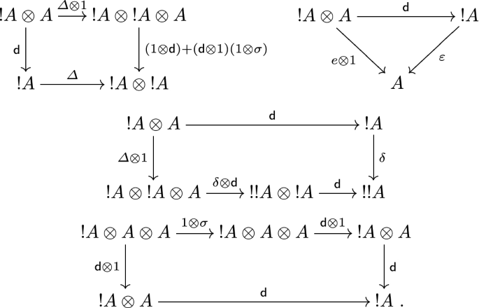
  $$\begin{aligned} \mathsf {d}_A :{!}A \otimes A \rightarrow {!}A \end{aligned}$$

  rendering commutative the following diagrams, known respectively as the product rule, the linear rule, the chain rule and the interchange rule.

  

  We call ${{\mathcal {V}}}$ endowed with its differential modality a tensor differential category.

• We call ! a monoidal differential modality if it is a monoidal coalgebra modality endowed with a deriving transformation.⁴

The above notion of deriving transformation refines that of [7] in two standard ways. Firstly, it drops the constant rule (“[d.1]” in loc. cit.) since this is derivable as in [6, Lemma 4.2]. Secondly, it adds the interchange rule, which is necessary to ensure that the following result holds without further side-conditions:

Proposition 4.4

Let ${{\mathcal {V}}}$ be a symmetric monoidal category k-linear category with finite (bi)products. For any differential modality ! on ${{\mathcal {V}}}$, the co-Kleisli category ${\mathcal {K}}\mathrm{l}({!})$ has a structure of cartesian differential category. If ${{\mathcal {V}}}$ is monoidal closed and ! is monoidal, then ${\mathcal {K}}\mathrm{l}(!)$ is a cartesian closed differential category.

Proof

The first assertion is [8, Lemmas 3.2.2 and 3.2.3]. The claim in the final sentence is [4, Theorem 4.4.2]. $\square$

While there is no need to recount the proof of this result, we will need to know how the cartesian differential structure of ${\mathcal {K}}\mathrm{l}(!)$ is obtained. The cartesian left-k-linear structure is easy: the hom ${\mathcal {K}}\mathrm{l}({!})(A,B)$ inherits k-module structure from ${{\mathcal {V}}}({!}A, B)$, and finite products in ${\mathcal {K}}\mathrm{l}(!)$ are induced from those of ${{\mathcal {V}}}$ along the identity-on-objects right adjoint functor ${{\mathcal {V}}}\rightarrow {\mathcal {K}}\mathrm{l}(!)$. As for the differential structure, if $f :{!}A \rightarrow B$ is a map in ${\mathcal {K}}\mathrm{l}(!)(A,B)$, then $\mathrm {D}f \in {\mathcal {K}}\mathrm{l}(!)(A \times A, B)$ is the composite

(16)

whose first part is the storage map of (14). When ! is monoidal and ${{\mathcal {V}}}$ is monoidal closed, the exponentials making ${\mathcal {K}}\mathrm{l}({!})$ cartesian closed are given by $B^A \mathrel {\mathop :}=[{!}A, B]$.

Definition 4.5

If ! is the differential modality of a tensor differential category, and ${{\mathcal {A}}}$ is a cartesian differential category, then we say that ${{\mathcal {A}}}$ is induced by ! if ${{\mathcal {A}}}\cong {\mathcal {K}}\mathrm{l}({!})$ as cartesian differential categories.

An extremely important source of differential modalities, and hence of cartesian differential categories, is the following result:

Proposition 4.6

Let ${{\mathcal {V}}}$ be a symmetric monoidal k-linear category with finite biproducts, and suppose the forgetful functor ${\mathcal {C}}\mathrm{ocomon}({{\mathcal {V}}}) \rightarrow {{\mathcal {V}}}$ has a right adjoint. The induced cofree cocommutative coalgebra comonad R on ${{\mathcal {V}}}$ can be made into a differential modality which is terminal among differential modalities on ${{\mathcal {V}}}$.

Proof

It is well-known that R is a monoidal coalgebra modality; indeed, this is the basis for Lafont’s semantics for the exponential modality of linear logic. The construction of a deriving transformation for ${{\mathcal {V}}}$ is given (in dual form) in [5, § 4], while § 6 of loc. cit. proves its terminality among differential modalities.⁵$\square$

Examples 4.7

(i) Taking ${{\mathcal {V}}}= k\text{- }{\mathcal {M}}\mathrm{od}^\mathrm {op}$ in the preceding result, we see that the free symmetric algebra monad $\mathrm {Sym}$ of (2) endows $k\text{- }{\mathcal {M}}\mathrm{od}^\mathrm {op}$ with a differential modality. The induced cartesian differential category is exactly the cartesian differential category ${\mathcal {G}}\mathrm{en}{{\mathcal {P}}}\mathrm{oly}_k$ of Examples 2.3(v), while ${\mathcal {P}}\mathrm{oly}_k$ is its full subcategory on the finitely generated free k-modules.

(ii) When ${{\mathcal {V}}}= {\mathcal {R}}\mathrm{el}$, the category of sets and relations, the cofree cocommutative comonoid on X is given by the set of finite multisets of elements of X. So the finite multiset comonad on ${\mathcal {R}}\mathrm{el}$ is a differential modality; the induced cartesian differential category is described explicitly in [11, § 5.1].

(iii) When ${{\mathcal {V}}}= {\mathcal {F}}\mathrm{in}$, the category of finiteness spaces and finitary relations [19], the cofree cocommutative comonoid is again given by the set of finite multisets with finiteness structure as defined in [37]. The induced cartesian differential category is described in [11, § 5.2].

(iv) When ${{\mathcal {V}}}= k\text{- }{\mathcal {M}}\mathrm{od}$ for k an algebraically closed field of characteristic zero, the cofree cocommutative coalgebra on a k-vector space A is given by $\bigoplus _{x \in A} \mathrm {Sym}(A)$, where $\mathrm {Sym}(A)$ is the symmetric algebra on A as in (2). This follows from results of [42], and is spelt out in [39]. In this case, the differential modality structure, and the induced cartesian differential category, are discussed in [13].

Note that Proposition 4.6 produces monoidal differential modalities which, in the case of (ii), (iii) and (iv), reside on monoidal closed categories. Thus, by Proposition 4.4, the co-Kleisli categories of these latter examples are cartesian closed differential categories. There are also important differential modalities which are not monoidal, for example on the category of $C^\infty$-rings; see [7, § 3] and [17].

Lastly, it may be worth mentioning that monoidal differential modalities have an alternative axiomatisation as monoidal coalgebra modalities equipped with a codereliction; this is a natural transformation ${\eta :A \rightarrow {!}A}$ satisfying certain identities which correspond to evaluating the differential at zero [6, 7, 20, 23]. These identities involve the canonical maps

(17)

definable in any monoidal coalgebra modality on a symmetric monoidal k-linear category, which together with $\varDelta$ and e endow each object !A with bialgebra structure. These same bialgebra maps are involved in the bijective correspondence between deriving transformations and coderelictions, due to [6, Theorem 4]. Indeed, the deriving transformation corresponding to a codereliction $\eta :A \rightarrow {!}A$ is given by:

while the codereliction of a deriving transformation $\mathsf {d}:{!}A \otimes A \rightarrow {!}A$ is given by

While the formulation in terms of a codereliction is more common in the literature on differential linear logic, for the purposes of the present paper it will be deriving transformations which are the focus; the algebra structure maps u and $\nabla$ and codereliction $\eta$ will play no subsequent role.

4.3 $\mathsf {Fa} \grave{\mathsf {a} }(k\text{- }{\mathcal {M}}\mathrm{od}_w)$ as a Co-Kleisli Construction

In this section, we show that, for the primordial left-k-linear category $k\text{- }{\mathcal {M}}\mathrm{od}_w$, its cofree cartesian differential category $\mathsf {Fa} \grave{\mathsf {a} }(k\text{- }{\mathcal {M}}\mathrm{od}_w)$ is induced by a particular (monoidal) differential modality Q on $k\text{- }{\mathcal {M}}\mathrm{od}$. To obtain Q, we could work backwards from $\mathsf {Fa} \grave{\mathsf {a} }(k\text{- }{\mathcal {M}}\mathrm{od}_w)$ using the results of [4], but it will be more illuminating to describe it directly.

In fact, we have already seen the formula for Q in Examples 2.5(iv); there, k was an algebraically closed field of characteristic zero, and the formula $\bigoplus _{x \in A} \mathrm {Sym}(A)$ in question gave the terminal differential modality on $k\text{- }{\mathcal {M}}\mathrm{od}$. For more general k, it turns out that this formula still describes a differential modality Q on $k\text{- }{\mathcal {M}}\mathrm{od}$, but the universal property is different: it is the initial monoidal differential modality.

For the purposes in this paper, we will not actually require this universal property, and so we reserve the proof of Q’s initiality for a follow-up paper—where it will be considered in a more general context—and content ourselves here with giving the explicit formulae. Note that these extend the ones given in [13] for k an algebraically closed field of characteristic zero.

Definition 4.8

The initial monoidal differential modality Q on $k\text{- }{\mathcal {M}}\mathrm{od}$ is given as follows.

• On objects, we have $QA = \textstyle \bigoplus _{x \in A} \mathrm {Sym}(A)$. We will write ${\langle {x_0, \ldots , x_n}\rangle } \in QA$ for the image of the pure tensor $x_1 \otimes \cdots \otimes x_n \in A^{\otimes n}$ under the composite

  

  of the quotient map and two coproduct injections. In particular, when $n = 0$, we write ${\langle {x_0}\rangle }$ for the image of $1 \in A^{\otimes 0}$ under the displayed composite. Note that the assessment $x_0, \ldots , x_n \mapsto {\langle {x_0, \ldots , x_n}\rangle }$ is symmetric multilinear in $x_1, \ldots , x_n$ but not $x_0$.

• On a map $f :A \rightarrow B$, we determine $Qf :QA \rightarrow QB$ by

  $$\begin{aligned} {\langle {x_0, \ldots , x_n}\rangle } \mapsto {\langle {f(x_0), \ldots , f(x_n)}\rangle }{ .} \end{aligned}$$

• For the comonad structure, the counit $\varepsilon _A :QA \rightarrow A$ is determined by

  $$\begin{aligned} {\langle {x_0}\rangle } \mapsto x_0\text { ,} \quad {\langle {x_0, x_1}\rangle } \mapsto x_1 \qquad \text {and} \quad {\langle {x_0, \ldots , x_n}\rangle } \mapsto 0 \text { if } n \geqslant 2. \end{aligned}$$

  and the comultiplication $\delta _A :QA \rightarrow QQA$ is determined by

  $$\begin{aligned} {\langle {x_0, \ldots , x_n}\rangle } \mapsto \sum _{[n] = A_1 \mid \cdots \mid A_k} {\langle { {\langle {x_0}\rangle }, {\langle {x_{A_1}}\rangle }, \ldots , {\langle {x_{A_k}}\rangle } }\rangle } \end{aligned}$$

  for $n \geqslant 0$. Here, as in Sect. 3, the sum is over unordered partitions of [n]; and we write ${\langle {x_{I}}\rangle }$ for ${\langle {x_0, x_{i_1}, \ldots , x_{i_k}}\rangle }$. Note in particular that $\delta _A({\langle {x_0}\rangle }) = {\langle {{\langle {x_0}\rangle }}\rangle }$.

• For the coalgebra modality structure, the comonoid counit $e_A :QA \rightarrow k$ is determined by

  $$\begin{aligned} {\langle {x_0}\rangle } \mapsto 1 \quad \text {and} \quad {\langle {x_0, \ldots , x_n}\rangle } \mapsto 0 \text { if } n \geqslant 1, \end{aligned}$$

  while the comultiplication map $\varDelta _A :QA \rightarrow QA \otimes QA$ is determined by

  $$\begin{aligned} {\langle {x_0,\ldots , x_n}\rangle } \mapsto \textstyle \sum _{I \subseteq [n]} {\langle {x_I}\rangle } \otimes {\langle {x_{[n] {\setminus } I}}\rangle }{ .} \end{aligned}$$

• For the monoidal structure, the nullary constraint $m_I :k \rightarrow Qk$ is determined by the assignment $1 \mapsto {\langle {1}\rangle }$, while the binary constraint $m_\otimes :QA \otimes QB \rightarrow Q(A \otimes B)$ is determined as follows (using the conventions of Notation 3.10 above):

  $$\begin{aligned} {\langle {x_0, \ldots , x_n}\rangle } \otimes {\langle {y_0, \ldots , y_m}\rangle } \mapsto \sum _{\theta :[n] \simeq [m]} {\langle {x_{\theta _{(1)}} \otimes y_{\theta _{(2)}}}\rangle }{ .} \end{aligned}$$

• Finally, the deriving transformation $\mathsf {d}_A :QA \otimes A \rightarrow QA$ is determined by

  $$\begin{aligned} {\langle {x_0,\ldots , x_n}\rangle } \otimes y \mapsto {\langle {x_0, \ldots , x_n, y}\rangle }{ .} \end{aligned}$$

The reader should have no trouble checking the axioms showing that $(Q, \varepsilon , \delta )$ as described above is a comonad; that the maps $(e, \varDelta )$ endow it with the structure of a coalgebra modality; and that $\mathsf {d}$ satisfies the deriving transformation axioms. It is then an interesting exercise to obtain the given form of the monoidal structure maps by first showing that the storage maps (14) for Q are invertible, and then deriving $m_I$ and $m_\otimes$ via the formulae (15). For the sake of completeness, we also note that:

• The bialgebra maps (17) have the unit $u_A:k \rightarrow QA$ determined by $1 \mapsto {\langle {0,1}\rangle }$ and the multiplication $\nabla :QA \otimes QA \rightarrow QA$ determined by

  $$\begin{aligned} {\langle {x_0,\ldots , x_n}\rangle } \otimes {\langle {y_0,\ldots , y_m}\rangle } \mapsto {\langle {x_0 + y_0,x_1, \ldots , x_n, y_1, \ldots , y_m}\rangle }{ .} \end{aligned}$$

• The codereliction map $\eta _A :A \rightarrow QA$ is given by $x \mapsto {\langle {0,x}\rangle }$.

Proposition 4.9

The cartesian differential category $\mathsf {Fa} \grave{\mathsf {a} }(k\text{- }{\mathcal {M}}\mathrm{od}_w)$ is induced by the initial monoidal differential modality Q on $k\text{- }{\mathcal {M}}\mathrm{od}$.

Proof

Clearly, objects of ${\mathcal {K}}\mathrm{l}(Q)$ and $\mathsf {Fa} \grave{\mathsf {a} }(k\text{- }{\mathcal {M}}\mathrm{od}_w)$ are the same. On maps, since

$$\begin{aligned} QA = \textstyle \bigoplus _{a \in A} SA = \bigoplus _{a \in A}(\bigoplus _{n \in \mathbb {N}}A^{\otimes n} / \mathfrak {S}_n) \cong \bigoplus _{n \in \mathbb {N}}(\bigoplus _{a \in A}A^{\otimes n} / \mathfrak {S}_n){ ,} \end{aligned}$$

we have a bijection between maps $A \rightarrow B$ in ${\mathcal {K}}\mathrm{l}(Q)$ and in $\mathsf {Fa} \grave{\mathsf {a} }(k\text{- }{\mathcal {M}}\mathrm{od}_w)$ by sending the k-linear map $f :QA \rightarrow B$ to the family of functions $f^{(\bullet )} :A \times A^n \rightarrow B$ with

$$\begin{aligned} f^{(n)}(x_0, \ldots , x_n) = f({\langle {x_0, \ldots , x_n}\rangle }){ .} \end{aligned}$$

(18)

It is clear from the formula for $\varepsilon _A :QA \rightarrow A$ that identity maps correspond under this bijection. As for composition, we can read off from the formulae for $\delta _A$ and Qf that the co-Kleisli composite of $f :QA \rightarrow B$ and $g :QB \rightarrow C$ is given by

$$\begin{aligned} {\langle {x_0, \ldots , x_n}\rangle } \quad \mapsto \quad \sum _{[n] = A_1 \mid \cdots \mid A_k} g{\langle { \,f{\langle {x_0}\rangle }, f{\langle {x_{A_1}}\rangle }, \ldots , f{\langle {x_{A_k}}\rangle }\,}\rangle }{ .} \end{aligned}$$

Transforming this via the formula (18) and comparing with (7), we conclude that this co-Kleisli composite corresponds to the Faá di Bruno composite $(g \circ f)^{(\bullet )}$. So we have an isomorphism of categories ${\mathcal {K}}\mathrm{l}(Q) \cong \mathsf {Fa} \grave{\mathsf {a} }(k\text{- }{\mathcal {M}}\mathrm{od}_w)$ which it is an easy exercise to check is an isomorphism of cartesian left-k-linear categories.

Finally, we compare the differentials $\mathrm {D}$. For ${\mathcal {K}}\mathrm{l}(Q)$, this is computed via formula (16); taking the image of a basis element of $Q(A \oplus A)$ under each of the maps in this composite in succession yields:

$$\begin{aligned}&{\langle {(x_0, y_0), \ldots , (x_n, y_n)}\rangle } {} \mapsto \textstyle \sum _{I \subseteq [n]} {\langle {x_I}\rangle } \otimes {\langle {y_{[n] {\setminus } I}}\rangle }\\&\quad {} \mapsto {\langle {x_0, \ldots , x_n}\rangle } \otimes y_0 + \textstyle \sum _{i=1}^n {\langle {x_0, \ldots , x_{i-1}, x_{i+1}, \ldots , x_n}\rangle } \otimes y_i \\&\quad {} \mapsto {\langle {x_0, \ldots , x_n, y_0}\rangle } + \textstyle \sum _{i=1}^n {\langle {x_0, \ldots , x_{i-1}, y_i, x_{i+1}, \ldots x_n}\rangle } \end{aligned}$$

Transforming this via (18) and comparing with (10), we conclude that ${\mathcal {K}}\mathrm{l}(Q) \cong \mathsf {Fa} \grave{\mathsf {a} }(k\text{- }{\mathcal {M}}\mathrm{od}_w)$ as cartesian differential categories. $\square$

We remark in passing that, since $k\text{- }{\mathcal {M}}\mathrm{od}$ is symmetric monoidal closed, and Q is a monoidal differential modality, $\mathsf {Fa} \grave{\mathsf {a} }(k\text{- }{\mathcal {M}}\mathrm{od}_w) \cong {\mathcal {K}}\mathrm{l}(Q)$ is a cartesian closed differential category, with the exponential $B^A$ of $A,B \in \mathsf {Fa} \grave{\mathsf {a} }(k\text{- }{\mathcal {M}}\mathrm{od}_w)$ given by the k-module of Faà di Bruno maps $A \rightsquigarrow B$.

4.4 $\mathsf {Fa} \grave{\mathsf {a} }({{\mathcal {A}}})$ as a Co-Kleisli Construction

We now show that, for a general left-k-linear category ${{\mathcal {A}}}$, there is a full structure-preserving embedding of $\mathsf {Fa} \grave{\mathsf {a} }({{\mathcal {A}}})$ into a cartesian differential category induced by a (monoidal) differential modality.

Definition 4.10

Let ${{\mathcal {A}}}$ be a left-k-linear category. We write ${\mathcal {P}}\mathrm{sh}_\ell ({{\mathcal {A}}})$ for the category $[{{\mathcal {A}}}^\mathrm {op}, k\text{- }{\mathcal {M}}\mathrm{od}]$ of $k\text{- }{\mathcal {M}}\mathrm{od}$-valued presheaves on the underlying ordinary category of ${{\mathcal {A}}}$ (the nomenclature will be explained in Sect. 7.2 below). The left-k-linearity of ${{\mathcal {A}}}$ endows each representable ${{\mathcal {A}}}({\mathord {-}}, A) :{{\mathcal {A}}}^\mathrm {op} \rightarrow {\mathcal {S}}\mathrm{et}$ with a lifting through the forgetful functor $k\text{- }{\mathcal {M}}\mathrm{od}\rightarrow {\mathcal {S}}\mathrm{et}$, and we write $yA \in {\mathcal {P}}\mathrm{sh}_\ell ({{\mathcal {A}}})$ for the object so obtained.

We view ${\mathcal {P}}\mathrm{sh}_\ell ({{\mathcal {A}}})$ as a symmetric monoidal k-linear category, where both the monoidal structure and the k-linear structure on the homs is given componentwise. With respect to this structure, we have a monoidal differential modality on ${\mathcal {P}}\mathrm{sh}_\ell ({{\mathcal {A}}})$ which is induced by postcomposition with the initial monoidal differential modality Q on $k\text{- }{\mathcal {M}}\mathrm{od}$. We call this the pointwise initial monoidal differential modality, and denote it by abuse of notation by Q.

Definition 4.11

Let ${{\mathcal {A}}}$ be a cartesian left-k-linear category. We write ${\mathcal {K}}\mathrm{l}_{{\mathcal {A}}}(Q)$ for the full subcategory of the co-Kleisli category of the pointwise initial monoidal differential modality Q on ${\mathcal {P}}\mathrm{sh}_\ell ({{\mathcal {A}}})$ on those objects of the form yA.

Note that we have $y(A \times B) \cong yA \times yB$, so that ${\mathcal {K}}\mathrm{l}_{{\mathcal {A}}}(Q)$ is closed under finite products in the full co-Kleisli category, and so is itself a cartesian differential category. Our objective is to show it is isomorphic to $\mathsf {Fa} \grave{\mathsf {a} }({{\mathcal {A}}})$; the key to which is a characterisation of objects of the form $Q(yA) \in {\mathcal {P}}\mathrm{sh}_\ell ({{\mathcal {A}}})$. Towards this, we give:

Definition 4.12

Let ${{\mathcal {A}}}$ be a cartesian left-k-linear category, and let $X \in {\mathcal {P}}\mathrm{sh}_\ell ({{\mathcal {A}}})$.

• (i) We say that $x \in XA$ is k-linear if each of the following functions is k-linear:

  $$\begin{aligned} \begin{aligned} {{\mathcal {A}}}(B,A)&\rightarrow XB \\ f&\mapsto Xf(x){ .} \end{aligned} \end{aligned}$$

  (19)

  In other words, writing $x \cdot f$ for Xf(x), we have $x \cdot (\lambda f+\mu g) = \lambda (x\cdot f) + \mu (x \cdot g)$.

• (ii) We say that $x \in X(A_1 \times \cdots \times A_n)$ is k-linear in the ith variable if it is k-linear as an element of the presheaf $X(A_1 \times \cdots \times A_{i-1} \times ({\mathord {-}}) \times A_{i+1} \times \cdots \times A_n)$.

• (iii) We say that $x \in X(A \times B^n)$ is symmetric in the last n variables if it is fixed by $X(1 \times \sigma )$ for all permutations $\sigma :B^n \rightarrow B^n$ of the product factors.

• (iv) A Faà di Bruno sequence of X at stage A is a family of elements

  $$\begin{aligned} \bigl (x^{(n)} \in X(A \times A^n) : n \in \mathbb {N}\bigr ) \end{aligned}$$

  such that each $x^{(n)}$ is symmetric and multilinear in its last n variables.

Lemma 4.13

Let ${{\mathcal {A}}}$ be a cartesian k-linear category, and let $A \in {{\mathcal {A}}}$. The object $Q(yA) \in {\mathcal {P}}\mathrm{sh}_\ell ({{\mathcal {A}}})$ classifies Faà di Bruno sequences at stage A. More precisely, the following family of elements is a Faà di Bruno sequence

$$\begin{aligned} {\langle {\pi _0, \ldots , \pi _n}\rangle } \in Q\bigl ({{\mathcal {A}}}(A \times A^n, A)\bigr ) = Q(yA)(A \times A^n){ ,} \end{aligned}$$

(20)

and for any $X \in {\mathcal {P}}\mathrm{sh}_\ell ({{\mathcal {A}}})$ and Faà di Bruno sequence $x^{(\bullet )}$ of X at stage A, there is a unique $\xi :Q(yA) \rightarrow X$ in ${\mathcal {P}}\mathrm{sh}_\ell ({{\mathcal {A}}})$ such that $\xi ({\langle {\pi _0, \ldots , \pi _{n}}\rangle }) = x^{(n)}$ for each n.

Proof

We first verify that the elements (20) constitute a Faà di Bruno sequence. For any sequence of maps $(f_0, \ldots , f_n) :B \rightarrow A^n$ in ${{\mathcal {A}}}$, we have that

$$\begin{aligned} {\langle {\pi _0,\ldots , \pi _{n}}\rangle } \cdot (f_0, \ldots , f_n) = {\langle {f_0,\ldots , f_n}\rangle } \in Q (yA)(B){ ;} \end{aligned}$$

(21)

Since for each $f_0$ the assignment $f_1, \ldots , f_n \mapsto {\langle {f_0, \ldots , f_n}\rangle }$ is symmetric multilinear, we see that ${\langle {\pi _0, \ldots , \pi _{n}}\rangle }$ is symmetric multilinear in its last n variables, as desired.

We now show universality of (20). Given $x^{(\bullet )}$ a Faà di Bruno sequence of $X \in {\mathcal {P}}\mathrm{sh}_\ell ({{\mathcal {A}}})$ at stage A, we define $\xi :Q(yA) \rightarrow X$ in ${\mathcal {P}}\mathrm{sh}_\ell ({{\mathcal {A}}})$ to have components

$$\begin{aligned} Q{{\mathcal {A}}}(B, A)&\rightarrow XB \\ {\langle {f_0, \ldots , f_n}\rangle }&\mapsto x^{(n)} \cdot (f_0, f_1, \ldots , f_n){ .} \end{aligned}$$

These are well-defined linear maps because of the symmetric multilinearity of x in its last n variables, and $\xi ({\langle {\pi _0, \ldots , \pi _n}\rangle }) = x^{(n)} \cdot (\pi _0, \pi _1, \ldots , \pi _n) = x^{(n)} \in X(A \times A^n)$. Moreover, if $\gamma :Q(yA) \rightarrow X$ in ${\mathcal {P}}\mathrm{sh}_\ell ({{\mathcal {A}}})$ satisfies $\gamma ({\langle {\pi _0, \ldots , \pi _n}\rangle }) = x^{(n)}$ for each n, then we have $\gamma ({\langle {f_0, \ldots , f_n}\rangle }) = \gamma ({\langle {\pi _0, \ldots , \pi _n}\rangle }) \cdot (f_0, \ldots , f_n) = x^{(n)} \cdot (f_0, f_1, \ldots , f_n)$ by (21) and naturality of $\gamma$, so that $\gamma = \xi$ as required. $\square$

Given this result, it is now straightforward to prove:

Proposition 4.14

Let ${{\mathcal {A}}}$ be a left-k-linear category. We have an isomorphism of cartesian differential categories $\mathsf {Fa} \grave{\mathsf {a} }({{\mathcal {A}}}) \cong {\mathcal {K}}\mathrm{l}_{{\mathcal {A}}}(Q)$, so that $\mathsf {Fa} \grave{\mathsf {a} }({{\mathcal {A}}})$ admits a full structure-preserving embedding into the cartesian differential category induced by the pointwise initial monoidal differential modality Q on ${\mathcal {P}}\mathrm{sh}_\ell ({{\mathcal {A}}})$.

Proof

Clearly, objects of $\mathsf {Fa} \grave{\mathsf {a} }({{\mathcal {A}}})$ and ${\mathcal {K}}\mathrm{l}_{{\mathcal {A}}}(Q)$ are the same. Now maps from A to B in ${\mathcal {K}}\mathrm{l}_{{\mathcal {A}}}(Q)$ are maps $f :Q yA \rightarrow yB$ in ${\mathcal {P}}\mathrm{sh}_\ell ({{\mathcal {A}}})$; by Lemma 4.13, these correspond to Faà di Bruno sequences of yB at stage A, whose data is precisely that of a map $f^{(\bullet )} :A \rightsquigarrow B$ in $\mathsf {Fa} \grave{\mathsf {a} }({{\mathcal {A}}})$. Observe that this $f^{(\bullet )}$ is characterised by

$$\begin{aligned} f^{(n)}(x_0, \ldots , x_n) = f({\langle {x_0, \ldots , x_n}\rangle }) \in {{\mathcal {A}}}(B,A) \end{aligned}$$

for all $X \in {{\mathcal {A}}}$ and $x_0, \ldots , x_n :X \rightarrow A$; noting the formal similarity to (18), we can thus conclude by transcribing the remainder of the proof of Proposition 4.9. $\square$

5 Enrichment Over Skew Monoidal Categories

We have just seen how to use the initial monoidal differential modality Q on $k\text{- }{\mathcal {M}}\mathrm{od}$ to construct cofree cartesian differential categories. This suggests that the notion of cartesian differential category is somehow controlled by the comonad Q; and the main result of the paper, to be proved in the next section, will show that this is indeed the case. There, we will see that that cartesian differential categories arise as categories enriched over $k\text{- }{\mathcal {M}}\mathrm{od}$ for a monoidal structure which is not the usual one, but rather a certain “warping” of it controlled by the comonad Q.

As explained in the introduction, a slight complication is that this warping is no longer a monoidal structure in the usual sense, but rather a skew monoidal structure in the sense of Szlachányi [43]. Since skew monoidal structures, and categories enriched over them, are likely to be unfamiliar to many, we devote this section to developing the necessary notions. We note that Sects. 5.1 and 5.2 are revision from [12, 41, 43], but Sects. 5.3–5.5 are novel (though straightforward).

5.1 Skew Monoidal Categories

A skew monoidal category generalises a monoidal category by dropping the requirement that the associativity and unitality constraint maps be invertible. Of course, it then matters how we choose to orient these maps, and “skew monoidal” refers to the following particular choice.

Definition 5.1

[43] A skew monoidal category is a category ${{\mathcal {V}}}$ endowed with a tensor product $\otimes :{{\mathcal {V}}}\times {{\mathcal {V}}}\rightarrow {{\mathcal {V}}}$ and unit object $I \in {{\mathcal {V}}}$, together with natural families

$$\begin{aligned} \alpha _{ABC} :(A \otimes B) \otimes C \rightarrow A \otimes (B \otimes C) \qquad \lambda _A :I \otimes A \rightarrow A \qquad \rho _A :A \rightarrow A \otimes I \end{aligned}$$

of maps satisfying the Mac Lane associativity pentagon, the condition $\lambda _I \circ \rho _I = 1_I$, and the three unit conditions (where we omit tensor symbols for compactness):

A skew monoidal category is said to be left closed if each functor $({\mathord {-}}) \otimes A :{{\mathcal {V}}}\rightarrow {{\mathcal {V}}}$ has a right adjoint $[A, {\mathord {-}}]$.

More precisely, we have just defined a left-skew monoidal category; a right-skew monoidal category reverses the directions of all three maps, but our convention will always be that “skew” means “left-skew”.

Example 5.2

Let $(M, +, 0)$ be a monoid. There is a left closed skew monoidal structure on ${\mathcal {S}}\mathrm{et}$ with unit $1 = \{*\}$, tensor product $A \times ^M B = A \times M \times B$, and constraint maps given as follows (where juxtaposition denotes cartesian product):

$$\begin{aligned} \lambda :1MB&\rightarrow B&\rho :A&\mapsto AM1&\alpha :(AMB)MC&\rightarrow AM(BMC) \\ (*, m, b)&\mapsto b&a&\mapsto (a,0,*)&((a,m,b),n,c)&\mapsto (a, m+n, (b, n, c)){ .} \end{aligned}$$

The associated internal hom is given by $B \Rightarrow ^M C = C^{M \times B}$.

This example is an instance of the following important construction, which builds skew monoidal structures from monoidal ones:

Definition 5.3

[43, Proposition 7.2] Let $({{\mathcal {V}}}, \otimes , I)$ be a monoidal category endowed with a monoidal comonad $({!}, \varepsilon , \delta , m_\otimes , m_I)$. The fusion operator [10, § 2.6] of !, which we use repeatedly in what follows, is the natural transformation H with components

(22)

The skew-warping of $\otimes$ with respect to ! is the skew monoidal structure on ${{\mathcal {V}}}$ with unit I, with tensor $A \otimes ^{!} B = A \otimes {!}B$ and with constraint cells

If the monoidal structure $(\otimes , I)$ is left closed, then so too is $(\otimes ^{!}, I)$, with the associated internal hom given by $[B, C]^{!} = [{!}B, C]$. We will often write⁶${{\mathcal {V}}}^{!}$ to denote ${{\mathcal {V}}}$ endowed with its warped skew monoidal structure $(\otimes ^!, I)$.

For example, if $(M,+,0)$ is a monoid, then $M \times ({\mathord {-}})$ is a monoidal comonad on ${\mathcal {S}}\mathrm{et}$, where $\varepsilon$ and $\delta$ involve projection and duplication, and $m_\otimes$ and $m_I$ involve the monoid structure of M. Instantiating Definition 5.3 at this monoidal comonad recovers the skew monoidal structure of Example 5.2.

The following further example provides a first indication of the relevance of skew monoidal structure to cartesian differential categories.

Example 5.4

Let ${{\mathcal {V}}}$ be a monoidal category with all copowers $X \cdot I \mathrel {\mathop :}=\sum _{x \in X} I$ of the unit I, whose tensor product preserves these copowers in the second variable. We have a monoidal adjunction

(23)

inducing a monoidal comonad K on ${{\mathcal {V}}}$; in fact, it is the initial monoidal comonad on ${{\mathcal {V}}}$. The warped monoidal structure $\otimes ^{K}$ is characterised by the fact that maps $A \otimes KB \rightarrow C$ are the same as functions ${{\mathcal {V}}}(I, B) \rightarrow {{\mathcal {V}}}(A,C)$. In particular, when ${{\mathcal {V}}}= k\text{- }{\mathcal {M}}\mathrm{od}$, maps $A \otimes ^K B \rightarrow C$ are exactly left-k-linear maps $A \times B \rightarrow C$.

5.2 Enrichment in a Skew Monoidal Category

We now turn to the notion of a category enriched in a skew monoidal category. Our definition follows Street [41, § 10], and mimics exactly the notion of enrichment over a genuine monoidal category. We remark that [12] gives a subtler notion of skew-enriched category, involving further extra data beyond the obvious. While there are good reasons to require these extra data, for our purposes it will prove unnecessary; though see Remark 7.3 below.

Definition 5.5

Let $({{\mathcal {V}}}, \otimes , I)$ be a skew monoidal category. A ${{\mathcal {V}}}$-enriched category ${{\mathcal {A}}}$ comprises the data of a set $\mathrm {ob}({{\mathcal {A}}})$ of objects; hom-objects ${{\mathcal {A}}}(A,B) \in {{\mathcal {V}}}$ for each $A,B \in \mathrm {ob}({{\mathcal {A}}})$; and composition and identity morphisms in ${{\mathcal {V}}}$

$$\begin{aligned} m_{ABC} :{{\mathcal {A}}}(B,C) \otimes {{\mathcal {A}}}(A,B) \rightarrow {{\mathcal {A}}}(A,C) \quad \text {and} \quad i_A :I \rightarrow {{\mathcal {A}}}(A,A){ ;} \end{aligned}$$

for all $A,B,C \in \mathrm {ob}({{\mathcal {A}}})$. These data are required to satisfy the axioms expressed by the commutativity of the diagrams

The underlying ordinary category ${{\mathcal {A}}}_0$ has the same objects as ${{\mathcal {A}}}$, hom-sets ${{\mathcal {A}}}_0(A,B) = {{\mathcal {V}}}(I, {{\mathcal {A}}}(A,B))$, and composition of $f \in {{\mathcal {A}}}_0(A,B)$ and $g \in {{\mathcal {A}}}_0(B,C)$ given by

(24)

We may speak of a map in ${{\mathcal {A}}}$ to mean a map in the underlying category ${{\mathcal {A}}}_0$.

Example 5.6

If the monoidal category ${{\mathcal {V}}}$ admits an initial monoidal comonad K as in Example 5.4, then we can consider categories enriched in the skew-warping ${{\mathcal {V}}}^{K}$. Such a category ${{\mathcal {A}}}$ involves a set of objects, hom-${{\mathcal {V}}}$-objects ${{\mathcal {A}}}(A,B)$, identities $I \rightarrow {{\mathcal {A}}}(A,A)$ and composition maps of the form

$$\begin{aligned} {{\mathcal {A}}}(B,C) \otimes ^K {{\mathcal {A}}}(A,B) \rightarrow {{\mathcal {A}}}(A,C){ .} \end{aligned}$$

In light of Example 5.4, it follows that when ${{\mathcal {V}}}= k\text{- }{\mathcal {M}}\mathrm{od}$ we recapture exactly the notion of left-k-linear category; this was observed in passing, and without any details being given, in [4, § 5.1].

In general, to give a ${{\mathcal {V}}}^K$-category is to give what we might call a left-${{\mathcal {V}}}$-enriched category: this is an ordinary category ${{\mathcal {A}}}_0$ together with, for each $B \in {{\mathcal {A}}}_0$, a lifting of the hom-functor ${{\mathcal {A}}}_0({\mathord {-}}, B) :{{\mathcal {A}}}_0^\mathrm {op} \rightarrow {\mathcal {S}}\mathrm{et}$ through ${{\mathcal {V}}}(I, {\mathord {-}})$:

5.3 Change of Enrichment Base

In classical enriched category theory, change of base allows us to turn a ${{\mathcal {V}}}$-enriched category into a ${{\mathcal {W}}}$-enriched one via a monoidal functor ${{\mathcal {V}}}\rightarrow {{\mathcal {W}}}$. This works just as well in the skew context.

Definition 5.7

A monoidal functor $(F, m_I, m_\otimes ) :{{\mathcal {V}}}\rightarrow {{\mathcal {W}}}$ between skew monoidal categories comprises a functor $F :{{\mathcal {V}}}\rightarrow {{\mathcal {W}}}$ together with a map $m_I :I \rightarrow FI$ and a natural family of maps $m_\otimes :FA \otimes FB \rightarrow F(A \otimes B)$, rendering commutative each of the diagrams:

If ${{\mathcal {A}}}$ is a ${{\mathcal {V}}}$-enriched category, then its base change $F_*{{\mathcal {A}}}$ is the ${{\mathcal {W}}}$-enriched category with the same objects, hom objects $(F_*{{\mathcal {A}}})(A,B) = F({{\mathcal {A}}}(A,B))$, and identities and composition given by

Examples 5.8

• (i) For any skew monoidal category ${{\mathcal {V}}}$ the functor ${{\mathcal {V}}}(I, {\mathord {-}}) :{{\mathcal {V}}}$ $\rightarrow {\mathcal {S}}\mathrm{et}$ is monoidal, where $m_I :1 \rightarrow {{\mathcal {V}}}(I,I)$ picks out the identity, and where the map $m_\otimes :{{\mathcal {V}}}(I,A) \times {{\mathcal {V}}}(I,B) \rightarrow {{\mathcal {V}}}(I,A \otimes B)$ takes f, g to the composite

  

  Base change along ${{\mathcal {V}}}(I,{\mathord {-}})$ sends a ${{\mathcal {V}}}$-category ${{\mathcal {A}}}$ to its underlying category ${{\mathcal {A}}}_0$.

• (ii) If ${{\mathcal {V}}}$ is a monoidal category and P, Q are monoidal comonads on ${{\mathcal {V}}}$, then each map of monoidal comonads $\gamma :P \rightarrow Q$ gives a monoidal functor $\mathrm {id} :{{\mathcal {V}}}^Q \rightarrow {{\mathcal {V}}}^P$ with nullary constraint $m_I$ the identity, and binary constraints given by

  

  This induces a base change operation ${{\mathcal {A}}}\mapsto \gamma ^*({{\mathcal {A}}})$ from ${{\mathcal {V}}}^Q$- to ${{\mathcal {V}}}^P$-categories; its only effect is to turn the composition maps ${{\mathcal {A}}}(B,C) \otimes Q{{\mathcal {A}}}(A,B) \rightarrow {{\mathcal {A}}}(A,C)$ into ones ${{\mathcal {A}}}(B,C) \otimes Q{{\mathcal {A}}}(A,B) \rightarrow {{\mathcal {A}}}(A,C)$ by precomposing with $1 \otimes \gamma$. For example, if ${{\mathcal {V}}}$ supports the initial monoidal comonad K, then the unique map to the terminal monoidal comonad $\mathrm {id}$, namely $\varepsilon :K \rightarrow \mathrm {id}$, gives a change of base functor from ${{\mathcal {V}}}$-enriched categories to left-${{\mathcal {V}}}$-enriched categories. In particular, this is how k-linear categories can be viewed as left-k-linear.

5.4 ${{\mathcal {V}}}$-Linear Maps in an Enriched Category

Since left-k-linear categories can be seen as categories enriched over a skew monoidal base, it is reasonable to ask if there is an analogue for a general skew monoidal enrichment of the notion of k-linear map. The answer is “yes”, but some care is needed: in full generality, being “linear” may be structure on a map, rather than a property of it.

Definition 5.9

Let ${{\mathcal {V}}}$ be a skew monoidal category, ${{\mathcal {A}}}$ a ${{\mathcal {V}}}$-enriched category and $A,B \in {{\mathcal {A}}}$. A ${{\mathcal {V}}}$-linear map $f :A \rightarrow _\ell B$ comprises maps $f_X :{{\mathcal {A}}}(X,A) \rightarrow {{\mathcal {A}}}(X,B)$ in ${{\mathcal {V}}}$ which are ${{\mathcal {V}}}$-natural, in the sense of rendering commutative each diagram

(25)

The underlying map $f_0 :A \rightarrow B$ of f is given by the composite

The objects and ${{\mathcal {V}}}$-linear maps form a category ${{\mathcal {A}}}_\ell$, and the assignment $f \mapsto f_0$ is the action on maps of an identity-on-objects functor ${{\mathcal {A}}}_\ell \rightarrow {{\mathcal {A}}}_0$.

When ${{\mathcal {V}}}$ is genuinely monoidal, a weak form of the Yoneda lemma shows that ${{\mathcal {V}}}$-linear maps are in bijection with maps of the underlying category, i.e., ${{\mathcal {A}}}_\ell \rightarrow {{\mathcal {A}}}_0$ is an isomorphism. However, in the skew case, it may not even be true that a ${{\mathcal {V}}}$-linear map f is determined by its underlying map $f_0$. The following is the diagram which would usually be drawn to prove this statement:

(26)

but in the skew context, $\lambda$ need not be invertible, so invalidating the formula $f_X = m \circ (f_0 \otimes 1) \circ \lambda ^{-1}$ which would determine $f_X$ from $f_0$.

Example 5.10

Let ${{\mathcal {V}}}$ be the monoidal category of $\mathbb {N}$-graded k-modules with its usual tensor product $(A \otimes B)_n = \sum _{n = p+q}A_p \otimes B_q$, and let ${{\mathcal {V}}}^K$ be its skew-warping for the initial monoidal comonad. A category ${{\mathcal {A}}}$ enriched over ${{\mathcal {V}}}^K$ has graded k-modules of maps ${{\mathcal {A}}}(A,B)$, identities $\mathrm {id}_A \in {{\mathcal {A}}}(A,A)_0$, and composition given by left-k-linear maps ${{\mathcal {A}}}(B,C)_n \times {{\mathcal {A}}}(A,B)_0 \rightarrow {{\mathcal {A}}}(A,C)_n$. The leading example is the category ${{\mathcal {A}}}$ whose objects are graded k-modules, and for which ${{\mathcal {A}}}(A,B)_n$ is the set of functions $A_0 \rightarrow B_n$. In this case, a map in the underlying category is simply a function $A_0 \rightarrow B_0$, while a ${{\mathcal {V}}}^K$-linear map can be calculated to be a genuine map of graded k-modules $A \rightarrow B$; clearly, the former does not determine the latter.

This leads us to make the following definition, which captures the situation in which ${{\mathcal {V}}}$-linearity is, in fact, a property rather than a structure:

Definition 5.11

A skew monoidal category $({{\mathcal {V}}}, \otimes , I)$ is called left covering if each map $\lambda _A :I \otimes A \rightarrow A$ is an epimorphism.

In this case, the standard Yoneda lemma argument via (26) now proves:

Lemma 5.12

If ${{\mathcal {V}}}$ is a left covering skew monoidal category, and ${{\mathcal {A}}}$ is a ${{\mathcal {V}}}$-category, then to give a ${{\mathcal {V}}}$-linear map $f :A \rightarrow _\ell B$ is equally to give a map $f_0 :A \rightarrow B$ in (the underlying category of) ${{\mathcal {A}}}$ for which each of the following factorisations exists:

(27)

In particular, when ${{\mathcal {V}}}$ is left covering, ${{\mathcal {A}}}_\ell \rightarrow {{\mathcal {A}}}_0$ is a faithful functor.

Example 5.13

If ! is a monoidal comonad on the monoidal category ${{\mathcal {V}}}$, then the skew-warping ${{\mathcal {V}}}^!$ is left covering just when each counit map $\varepsilon _X :!X \rightarrow X$ is epimorphic. In particular, if ${{\mathcal {V}}}$ admits the initial monoidal comonad K, then ${{\mathcal {V}}}^K$ is left covering precisely when the unit object I is a generator for ${{\mathcal {V}}}$.

In this case, if ${{\mathcal {A}}}$ is a ${{\mathcal {V}}}^K$-category, then a map $f \in {{\mathcal {A}}}_0(A,B)$ is ${{\mathcal {V}}}^K$-linear precisely when each composition function $f \circ ({\mathord {-}}) :{{\mathcal {A}}}_0(X,A) \rightarrow {{\mathcal {A}}}_0(X,B)$ is the image under the faithful functor ${{\mathcal {V}}}(I,{\mathord {-}}) :{{\mathcal {V}}}\rightarrow {\mathcal {S}}\mathrm{et}$ (faithful since I is a generator) of a map ${{\mathcal {A}}}(X,A) \rightarrow {{\mathcal {A}}}(X,B)$ in ${{\mathcal {V}}}$. In particular, when ${{\mathcal {V}}}= k\text{- }{\mathcal {M}}\mathrm{od}$, a ${{\mathcal {V}}}^K$-linear map is precisely a k-linear map in the sense of Definition 2.2.

5.5 Finite Products in an Enriched Category

Since we are interested in cartesian differential categories, we will need to understand the notion of finite product in the skew-enriched context. We conclude this section by discussing this.

Definition 5.14

Let ${{\mathcal {V}}}$ be a skew monoidal category and ${{\mathcal {A}}}$ a ${{\mathcal {V}}}$-enriched category.

• (i) An object $1 \in {{\mathcal {A}}}$ is terminal for ${{\mathcal {A}}}$ if ${{\mathcal {A}}}(X,1)$ is terminal in ${{\mathcal {V}}}$ for all $X \in {{\mathcal {A}}}$.

• (ii) A binary product of $A,B \in {{\mathcal {A}}}$ comprises an object $A \times B \in {{\mathcal {A}}}$ and a span of ${{\mathcal {V}}}$-linear maps $\pi _0 :A \leftarrow _\ell A \times B \rightarrow _\ell B :\pi _1$, with the property that each of the components ${{\mathcal {A}}}(X, A) \leftarrow {{\mathcal {A}}}(X, A \times B) \rightarrow {{\mathcal {A}}}(X, B)$ constitutes a product diagram in ${{\mathcal {V}}}$.

• (iii) ${{\mathcal {A}}}$ is cartesian when it has a terminal object and all binary products.

From Lemma 5.12 it follows immediately that:

Lemma 5.15

If ${{\mathcal {V}}}$ is a left covering skew monoidal category, then a ${{\mathcal {V}}}$-category ${{\mathcal {A}}}$ is cartesian just when its underlying ordinary category has finite products, and all binary product projections are ${{\mathcal {V}}}$-linear.

Example 5.16

A left-k-linear category ${{\mathcal {A}}}$ is cartesian qua $k\text{- }{\mathcal {M}}\mathrm{od}^K$-category precisely when it is cartesian left-k-linear.

6 Cartesian Differential Categories as Enriched Categories

In this section, we give the first main result of this paper, exhibiting cartesian differential categories as cartesian $k\text{- }{\mathcal {M}}\mathrm{od}^Q$-enriched categories, where Q is the initial monoidal differential modality of Definition 4.8.

6.1 Characterising $k\text{- }{\mathcal {M}}\mathrm{od}^Q$-Categories

Before proving the main theorem, we identify general $k\text{- }{\mathcal {M}}\mathrm{od}^Q$-categories; these turn out to be a variant of cartesian differential categories which do away with the need for finite products. An example of this notion would be the co-Kleisli category of the differential modality on a tensor differential category without finite products.

We first record an explicit description of the fusion map (22) for Q.

Lemma 6.1

The fusion map $H :QX \otimes QY \rightarrow Q(X \otimes QY)$ for the initial monoidal differential modality Q on $k\text{- }{\mathcal {M}}\mathrm{od}$ has action determined by

$$\begin{aligned} {\langle {x_0, \ldots , x_m}\rangle } \otimes {\langle {y_0, \ldots , y_n}\rangle } \quad \mapsto \quad \sum _{\begin{array}{c} [n] = A_1 \mid \cdots \mid A_k \\ \theta :[m] \simeq [k] \end{array}} {\langle { x_{\theta _{(1)}} \otimes {\langle {y_{A_{\theta _{(2)}}}}\rangle }}\rangle }{ ,} \end{aligned}$$

with the conventions of Notation 3.10, and with $A_0 \mathrel {\mathop :}=\emptyset$ so that ${\langle {y_{A_0}}\rangle } = {\langle {y_0}\rangle }$.

Proof

This can simply be read off from Definition 4.8. $\square$

Proposition 6.2

To give a $k\text{- }{\mathcal {M}}\mathrm{od}^Q$-enriched category ${{\mathcal {A}}}$ is equally to give a collection of objects; a k-module ${{\mathcal {A}}}(A,B)$ of maps between each pair of objects; identity elements $\mathrm {id}_A \in {{\mathcal {A}}}(A,A)$; and composition functions

$$\begin{aligned} \begin{aligned} {{\mathcal {A}}}(B,C) \times {{\mathcal {A}}}(A,B) \times {{\mathcal {A}}}(A,B)^n&\rightarrow {{\mathcal {A}}}(A,C) \\ (g, f_0, \ldots , f_n)&\mapsto g^{(n)}(f_0, \ldots , f_n) \end{aligned} \end{aligned}$$

(28)

for each $A,B,C \in {{\mathcal {A}}}$ and each $n \geqslant 0$, subject to the following axioms:

• (i) Each (28) is k-linear in g, and symmetric k-linear in $f_1, \ldots , f_n$;

• (ii) We have $g^{(0)}(\mathrm {id_A}) = g$;

• (iii) We have $\mathrm {id}_B^{(0)}(f) = f$, $\mathrm {id}_B^{(1)}(f_0, f_1) = f_1$ and $\mathrm {id}_B^{(n)}(f_0, \ldots , f_n) = 0$ for all $n \geqslant 2$;

• (iv) For all $f_0, \ldots , f_n :A \rightarrow B$, $g_0, \ldots , g_m :B \rightarrow C$ and $h :C \rightarrow D$ we have

  $$\begin{aligned} \displaystyle \bigl (h^{(m)}(g_0, \ldots , g_m)\bigr )^{(n)}(\mathbf {f}) = \sum _{\begin{array}{c} [n] = A_1 \mid \cdots \mid A_k\\ \theta :[m] \simeq [k] \end{array}} h^{({\left| {\theta }\right| })}\bigl (g_{\theta _{(1)}}^{(A_{\theta _{(2)}})}(\mathbf {f})\bigr ) { ,} \end{aligned}$$

  where we define $g_i^{(A_{j})}(\mathbf {f})$ as in (6).

Proof

A $k\text{- }{\mathcal {M}}\mathrm{od}^Q$-category ${{\mathcal {A}}}$ has objects $A,B,\ldots$; homs ${{\mathcal {A}}}(A,B) \in k\text{- }{\mathcal {M}}\mathrm{od}$; identity maps $i :k \rightarrow {{\mathcal {A}}}(A,A)$ which pick out elements $\mathrm {id}_A \in {{\mathcal {A}}}(A,A)$; and composition maps $m :{{\mathcal {A}}}(B,C) \otimes Q{{\mathcal {A}}}(A,B) \rightarrow {{\mathcal {A}}}(A,C)$, which, on writing their action as:

$$\begin{aligned} g \otimes {\langle {f_0, \ldots , f_n}\rangle } \mapsto g^{(n)}(f_0, \ldots , f_n){ ,} \end{aligned}$$

correspond to families of maps (28) satisfying axiom (i) in the statement. Now the right identity axiom for ${{\mathcal {A}}}$ requires commutativity of:

Chasing $g \in {{\mathcal {A}}}(A,B)$ around the long side we get $g \mapsto g \otimes {\langle {\mathrm {id}_A}\rangle } \mapsto g^{(0)}(\mathrm {id}_A)$, so that commutativity is exactly axiom (ii). Next, the left identity axiom requires commutativity in:

The upper composite takes ${\langle {f_0, \ldots , f_n}\rangle }$ to $\mathrm {id}_B^{(n)}(f_0, \ldots , f_n)$, and so comparing with the formula for $\varepsilon$, commutativity of this diagram is exactly axiom (iii). Finally, the associativity axiom requires commutativity in:

Chasing a generating element $h \otimes {\langle {g_0, \ldots , g_m}\rangle } \otimes {\langle {f_0, \ldots , f_n}\rangle }$ around the top composite yields $(h^{(m)}(g_0, \ldots , g_m))^{(n)}(\mathbf {f})$. On the other hand, chasing this generator around the lower composite yields in succession (using Lemma 6.1 at the first step):

$$\begin{aligned}&h \otimes {\langle {g_0, \ldots , g_m}\rangle } \otimes {\langle {f_0, \ldots , f_n}\rangle } \\&\quad \mapsto \sum _{\begin{array}{c} [n] = A_1 \mid \cdots \mid A_k \\ \theta :[m] \simeq [k] \end{array}} h \otimes {\langle { g_{\theta _{(1)}} \otimes {\langle {f_{A_{\theta _{(2)}}}}\rangle }}\rangle } \\&\quad \mapsto \sum _{\begin{array}{c} [n] = A_1 \mid \cdots \mid A_k \\ \theta :[m] \simeq [k] \end{array}} h \otimes {\langle { g_{\theta _{(1)}}^{(A_{\theta _{(2)}})}(\mathbf {f})}\rangle } \mapsto \sum _{\begin{array}{c} [n] = A_1 \mid \cdots \mid A_k \\ \theta :[m] \simeq [k] \end{array}} h^{({\left| {\theta }\right| })} \bigl ( g_{\theta _{(1)}}^{(A_{\theta _{(2)}})}(\mathbf {f})\bigr )\text {, } \end{aligned}$$

so that the associativity axiom is equivalent to axiom (iv) in the statement.

$\square$

6.2 Characterising Cartesian $k\text{- }{\mathcal {M}}\mathrm{od}^Q$-Categories

We now consider what it means for a $k\text{- }{\mathcal {M}}\mathrm{od}^Q$-category to have finite products; this will bridge the gap with cartesian differential categories. Note first that, since the counit maps $\varepsilon _X :QX \rightarrow X$ of Definition 4.8 are visibly epimorphic, $k\text{- }{\mathcal {M}}\mathrm{od}^Q$ is a left covering skew monoidal category. Thus, by Lemma 5.15, a $k\text{- }{\mathcal {M}}\mathrm{od}^Q$-category is cartesian just when its underlying ordinary category has finite products, and product projections are $k\text{- }{\mathcal {M}}\mathrm{od}^Q$-linear. The following result characterises this notion of linearity.

Proposition 6.3

A map $g :A \rightarrow B$ of a $k\text{- }{\mathcal {M}}\mathrm{od}^Q$-category ${{\mathcal {A}}}$ is $k\text{- }{\mathcal {M}}\mathrm{od}^Q$-linear just when, for all $X \in {{\mathcal {A}}}$ and $f_0, f_1, \ldots \in {{\mathcal {A}}}(X,A)$ we have:

$$\begin{aligned} g^{(1)}(f_0, f_1) = g^{(0)}(f_1) \quad \text {and} \quad g^{(n)}(f_0, \ldots , f_n) = 0\quad \text {for all}\quad n \geqslant 2. \end{aligned}$$

(29)

Proof

By Lemma 5.12, g is $k\text{- }{\mathcal {M}}\mathrm{od}^Q$-linear just when, for each $X \in {{\mathcal {A}}}$ there is a factorisation in $k\text{- }{\mathcal {M}}\mathrm{od}$ of the form

Evaluating both ways around the diagram at ${\langle {f_0}\rangle } \in Q{{\mathcal {A}}}(X,A)$, we must have $g_X(f_0) = g^{(0)}(f_0)$; evaluating at ${\langle {f_0, f_1}\rangle }$, we must have $g_X(f_1) = g^{(1)}(f_0, f_1)$; and evaluating at ${\langle {f_0, \ldots , f_n}\rangle }$ for $n \geqslant 2$, we must have $0 = g^{(n)}(f_0, \ldots , f_n)$. This shows the necessity of (29); the sufficiency follows on noting that $g_X$ defined thus is k-linear, since $g_X(f) = g^{(1)}(0,f)$ and $g^{(1)}$ is k-linear in its second argument. $\square$

We are now ready to prove the first main result of the paper.

Theorem 6.4

To give a cartesian differential category is equally to give a cartesian $k\text{- }{\mathcal {M}}\mathrm{od}^Q$-category; under this correspondence, the $\mathrm {D}$-linear maps correspond to the $k\text{- }{\mathcal {M}}\mathrm{od}^Q$-linear ones.

Proof

Consider first a cartesian differential category ${{\mathcal {A}}}$, presented as in Corollary 3.14. The corresponding $k\text{- }{\mathcal {M}}\mathrm{od}^Q$-category ${\underline{{{\mathcal {A}}}}}$ will have the same objects, hom-modules, and identity maps; while its composition functions (28) are defined using the higher-order derivatives and composition in ${{\mathcal {A}}}$. We obtain the various axioms of Proposition 6.2 as follows:

• (i) This follows from axioms (i) and (ii) of Corollary 3.14;

• (ii) This follows from the category axioms for ${{\mathcal {A}}}$;

• (iii) This follows from axiom (iv) of Corollary 3.14;

• (iv) This follows from the combination of axioms (v) and (vii) of Corollary 3.14.

To see that ${\underline{{{\mathcal {A}}}}}$ is cartesian, note that its underlying ordinary category—which is ${{\mathcal {A}}}$—admits finite products, and that the product projection maps $\pi _i$ are $k\text{- }{\mathcal {M}}\mathrm{od}^Q$-linear by axiom (iii) of Corollary 3.14.

Suppose conversely that ${\underline{{{\mathcal {A}}}}}$ is a cartesian $k\text{- }{\mathcal {M}}\mathrm{od}^Q$-category. By changing base along the unique monoidal comonad morphism $\gamma :K \rightarrow Q$, we see that ${\underline{{{\mathcal {A}}}}}$ has an underlying left-k-linear category ${{\mathcal {A}}}$, with the same objects, hom-objects and identities, and with composition law $g \circ f = g^{(0)}(f)$. Moreover, the finite products of ${\underline{{{\mathcal {A}}}}}$ yield finite products in ${{\mathcal {A}}}$, which is thus cartesian left-k-linear.

For each $n \geqslant 0$ and $A,B \in {{\mathcal {A}}}$, we now define the higher-order derivative

$$\begin{aligned} \begin{aligned} ({\mathord {-}})^{(n)} :{{\mathcal {A}}}(A,B)&\rightarrow {{\mathcal {A}}}(A \times A^n, B) \\ f&\mapsto f^{(n)}(\pi _0, \pi _1, \ldots , \pi _n) \end{aligned} \end{aligned}$$

(30)

on ${{\mathcal {A}}}$. We claim that these satisfy the axioms of Corollary 3.14, so yielding a cartesian differential structure on ${{\mathcal {A}}}$. Observe first that, given $f_0, \ldots , f_n :A \rightarrow B$ and $g :B \rightarrow C$, we can form $f = (f_0, \ldots , f_n) :A \rightarrow B \times B^n$ and now have

$$\begin{aligned} \begin{aligned} g^{(n)} \circ f&= (g^{(n)}(\pi _0, \pi _1, \ldots , \pi _n))^{(0)}(f) \\&= g^{(n)}(\pi _0^{(0)}(f), \ldots , \pi _n^{(0)}(f)) = g^{(n)}(f_0, \ldots , f_n){ ,} \end{aligned} \end{aligned}$$

(31)

recapturing the composition operation in ${\underline{{{\mathcal {A}}}}}$. In verifying the axioms of Corollary 3.14, we first translate them under (31) to axioms on the composition law (28) in $\underline{{{\mathcal {A}}}}$. On doing so, we find that:

• (i)–(ii) follow from condition (i) of Proposition 6.2;

• (iii) follows from the $k\text{- }{\mathcal {M}}\mathrm{od}^Q$-linearity of product projections in ${\underline{{{\mathcal {A}}}}}$;

• (iv) follows from axiom (iii) of Proposition 6.2;

• (v) follows from axiom (iv) of Proposition 6.2 on taking $m = 0$;

• (vi) follows from axiom (ii) of Proposition 6.2;

• (vii) follows from axiom (iv) of Proposition 6.2 on taking

  $$\begin{aligned}(g_0, \ldots , g_m) = (\pi _0, \ldots , \pi _m)\text { .}\end{aligned}$$

We have thus shown that there are assignments ${{\mathcal {A}}}\mapsto {\underline{{{\mathcal {A}}}}}$ and ${\underline{{{\mathcal {A}}}}} \mapsto {{\mathcal {A}}}$ between cartesian differential categories and cartesian $k\text{- }{\mathcal {M}}\mathrm{od}^Q$-categories, and it is now easy to see that these are mutually inverse: in one direction, we use (31), and in the other, the fact that $(\pi _0, \ldots , \pi _n) = \mathrm {id} :A \times A^n \rightarrow A \times A^n$.

Finally, Proposition 6.3 shows that, under the correspondence just given, the $k\text{- }{\mathcal {M}}\mathrm{od}^Q$-linear maps correspond to the $\mathrm {D}$-linear ones. $\square$

It is probably worth recording in as concrete a form as possible the two directions of our main correspondence. On the one hand, for a cartesian differential category ${{\mathcal {A}}}$, the corresponding $k\text{- }{\mathcal {M}}\mathrm{od}^Q$-category has the same objects, the same hom-k-modules, and the same identities; and has composition laws

$$\begin{aligned} {{\mathcal {A}}}(B,C) \otimes Q{{\mathcal {A}}}(A,B)&\rightarrow {{\mathcal {A}}}(A,C) \\ g \otimes {\langle {f_0, \ldots , f_n}\rangle }&\mapsto g^{(n)}(f_0, \ldots , f_n){ ,} \end{aligned}$$

where $g^{(n)}$ denotes the nth derivative of Definition 3.1. On the other hand, for a cartesian $k\text{- }{\mathcal {M}}\mathrm{od}^Q$-category ${{\mathcal {A}}}$, the corresponding cartesian differential category has the same objects, the same hom-k-modules and the same identities; while its composition and its differential operator are defined from the $k\text{- }{\mathcal {M}}\mathrm{od}^Q$-composition maps $m :{{\mathcal {A}}}(B, C) \otimes Q{{\mathcal {A}}}(A,B) \rightarrow {{\mathcal {A}}}(A,C)$ via

$$\begin{aligned} g \circ f = m(g \otimes {\langle {f}\rangle }) \quad \text {and} \quad \mathrm {D}f = m(f \otimes {\langle {\pi _0, \pi _1}\rangle }){ .} \end{aligned}$$

7 Presheaves Over a Skew Monoidal Base

In the rest of the paper, we will make use of our first main theorem to prove our second one: that every small cartesian differential category has a full structure-preserving embedding into one induced by a monoidal differential modality on a symmetric monoidal closed k-linear category. The embedding in question will be the Yoneda embedding into an enriched presheaf category, and so in this section we develop the appropriate notions in the skew context. We note that the definitions in this section draw largely on [41] with some novelties (the notions of tight ${{\mathcal {V}}}$-functor and the identification of the ${{\mathcal {V}}}$-linear presheaf maps); while the lemmas and propositions are all new.

7.1 Enriched Functors

So far, we have discussed categories enriched over a skew monoidal category in isolation. We will now need to discuss also functors between enriched categories. The obvious definition is the following one:

Definition 7.1

Let ${{\mathcal {V}}}$ be a skew monoidal category, and let ${{\mathcal {A}}}, {{\mathcal {B}}}$ be ${{\mathcal {V}}}$-categories. A ${{\mathcal {V}}}$-functor $F :{{\mathcal {A}}}\rightarrow {{\mathcal {B}}}$ comprises an assignment $A \mapsto FA$ from objects of ${{\mathcal {A}}}$ to those of ${{\mathcal {B}}}$, together with maps $F_{A,B} :{{\mathcal {A}}}(A,B) \rightarrow {{\mathcal {B}}}(FA,FB)$ in ${{\mathcal {V}}}$ for all $A,B \in {{\mathcal {A}}}$, which render commutative all diagrams of the following form:

However, for various purposes, this definition is insufficient. For example, we would like to say that a ${{\mathcal {V}}}$-functor preserves finite products just when it sends product cones to product cones. However, a ${{\mathcal {V}}}$-functor as defined above does not even induce a mapping on product cones, because it has no action on ${{\mathcal {V}}}$-linear maps. This motivates:

Definition 7.2

Let ${{\mathcal {V}}}$ be a skew monoidal category, and let ${{\mathcal {A}}}, {{\mathcal {B}}}$ be ${{\mathcal {V}}}$-categories. A tight ${{\mathcal {V}}}$-functor $F :{{\mathcal {A}}}\rightarrow _t {{\mathcal {B}}}$ is a ${{\mathcal {V}}}$-functor $F :{{\mathcal {A}}}\rightarrow {{\mathcal {B}}}$ together with an ordinary functor on categories of linear maps $F_\ell :{{\mathcal {A}}}_\ell \rightarrow {{\mathcal {B}}}_\ell$, such that for each $f :B \rightarrow _\ell C$ in ${{\mathcal {A}}}_\ell$ and $A \in {{\mathcal {A}}}$, the following diagram commutes:

Remark 7.3

This definition is based on ideas of [12]. If ${{\mathcal {V}}}$ is a skew monoidal category, then Campbell in loc. cit. defines a skew-enriched ${{\mathcal {V}}}$-category to comprise an ordinary category ${{\mathcal {A}}}_\ell$, together with a functor ${{\mathcal {A}}}({\mathord {-}}, {\mathord {-}}) :{{\mathcal {A}}}_\ell ^\mathrm {op} \times {{\mathcal {A}}}_\ell \rightarrow {{\mathcal {V}}}$ and maps $I \rightarrow {{\mathcal {A}}}(A,A)$ and ${{\mathcal {A}}}(B,C) \otimes {{\mathcal {A}}}(A,B) \rightarrow {{\mathcal {A}}}(A,C)$ which are natural in $A,B, C \in {{\mathcal {A}}}_\ell$, and satisfy the axioms of Definition 5.5. If ${{\mathcal {A}}}$ and ${{\mathcal {B}}}$ are ${{\mathcal {V}}}$-categories in our sense, then they become skew-enriched ${{\mathcal {V}}}$-categories in Campbell’s sense on taking ${{\mathcal {A}}}_\ell$ and ${{\mathcal {B}}}_\ell$ to be the categories of ${{\mathcal {V}}}$-linear maps; on doing so, the skew-enriched ${{\mathcal {V}}}$-functors between them, in Campbell’s sense, are precisely our tight ${{\mathcal {V}}}$-functors.

While tightness is, in general, extra structure on a ${{\mathcal {V}}}$-functor, in the left covering case which is of primary interest to us, it is a mere property.

Lemma 7.4

Let ${{\mathcal {V}}}$ be a left covering skew monoidal category, and let ${{\mathcal {A}}},{{\mathcal {B}}}$ be ${{\mathcal {V}}}$-categories. To give a tight ${{\mathcal {V}}}$-functor $F :{{\mathcal {A}}}\rightarrow _t {{\mathcal {B}}}$ is equally to give a ${{\mathcal {V}}}$-functor $F :{{\mathcal {A}}}\rightarrow {{\mathcal {B}}}$ whose underlying functor $F_0 :{{\mathcal {A}}}_0 \rightarrow {{\mathcal {B}}}_0$ preserves ${{\mathcal {V}}}$-linear maps.

Proof

A straightforward argument using Lemma 5.12. $\square$

Example 7.5

Let ${{\mathcal {A}}}$ and ${{\mathcal {B}}}$ be left-k-linear categories. A $k\text{- }{\mathcal {M}}\mathrm{od}^K$-functor between them is an ordinary functor $F :{{\mathcal {A}}}\rightarrow {{\mathcal {B}}}$ whose action on homs preserves the k-module structure. Such a functor is tight just when it preserves k-linear maps.

Using the notion of tightness, we can now describe what it means for a functor to preserve cartesian structure.

Definition 7.6

Let ${{\mathcal {V}}}$ be a skew monoidal category, and let ${{\mathcal {A}}}, {{\mathcal {B}}}$ be cartesian ${{\mathcal {V}}}$-categories. A tight ${{\mathcal {V}}}$-functor $F :{{\mathcal {A}}}\rightarrow _t {{\mathcal {B}}}$ is said to be cartesian if it sends terminal objects to terminal objects, and $F_\ell$ sends binary product cones $A \leftarrow _\ell A \times B \rightarrow _\ell B$ to binary product cones.

Example 7.7

Let ${{\mathcal {A}}}$ and ${{\mathcal {B}}}$ be cartesian differential categories, seen as cartesian $k\text{- }{\mathcal {M}}\mathrm{od}^Q$-categories. It is a straightforward calculation to see that a $k\text{- }{\mathcal {M}}\mathrm{od}^Q$-functor from ${{\mathcal {A}}}$ to ${{\mathcal {B}}}$ is an ordinary functor $F :{{\mathcal {A}}}\rightarrow {{\mathcal {B}}}$ which preserves addition on the homs, and for which each diagram of the following form commutes in ${{\mathcal {B}}}$:

Such a $k\text{- }{\mathcal {M}}\mathrm{od}^Q$-functor is tight precisely when it preserves $\mathrm {D}$-linearity of maps; and it is cartesian when, in addition, it preserves finite products in the usual sense. In fact, preservation of $\mathrm {D}$-linearity automatically implies preservation of finite products by the argument of [8, Lemma 1.3.2] (so in this sense finite products in $k\text{- }{\mathcal {M}}\mathrm{od}^Q$-categories are absolute limits).

7.2 Enriched Presheaves

We now describe the notion of presheaf on a category enriched over a skew monoidal category.

Definition 7.8

[41, § 5] Let ${{\mathcal {V}}}$ be a skew monoidal category and ${{\mathcal {A}}}$ a ${{\mathcal {V}}}$-enriched category. A presheaf X on ${{\mathcal {A}}}$ is given by objects $XA \in {{\mathcal {V}}}$ for each $A \in {{\mathcal {A}}}$, and maps $m :XB \otimes {{\mathcal {A}}}(A,B) \rightarrow XA$ for each $A,B \in {{\mathcal {A}}}$, rendering commutative each diagram

If X, Y are presheaves on ${{\mathcal {A}}}$, then a ${{\mathcal {V}}}$-linear presheaf map $f :X \rightarrow Y$ comprises families of maps $f_A :XA \rightarrow YA$ which commute with the ${{\mathcal {A}}}$-action, in the sense of rendering commutative each square

We write ${\mathcal {P}}\mathrm{sh}_{\ell }({{\mathcal {A}}})$ for the category of presheaves on ${{\mathcal {A}}}$ and ${{\mathcal {V}}}$-linear presheaf maps.

Example 7.9

If ${{\mathcal {A}}}$ is a ${{\mathcal {V}}}$-category, then for each $A \in {{\mathcal {A}}}$, we have a presheaf $yA \in {\mathcal {P}}\mathrm{sh}_\ell ({{\mathcal {A}}})$ with components $yA(B) = {{\mathcal {A}}}(B,A)$ and action given by composition in ${{\mathcal {A}}}$. Moreover, ${{\mathcal {V}}}$-linear presheaf maps $yA \rightarrow yB$ are precisely ${{\mathcal {V}}}$-linear maps $A \rightarrow _\ell B$ in ${{\mathcal {A}}}$.

Example 7.10

Let ${{\mathcal {V}}}$ be a monoidal category which supports the initial monoidal comonad K, and let ${{\mathcal {A}}}$ be a ${{\mathcal {V}}}^K$-enriched category. In this case, ${\mathcal {P}}\mathrm{sh}_\ell ({{\mathcal {A}}})$ is the ordinary functor category $[{{\mathcal {A}}}_0^\mathrm {op}, {{\mathcal {V}}}]$. In particular, if ${{\mathcal {A}}}$ is a left-k-linear category, then ${\mathcal {P}}\mathrm{sh}_\ell ({{\mathcal {A}}})$ is $[{{\mathcal {A}}}_0^\mathrm {op}, k\text{- }{\mathcal {M}}\mathrm{od}]$—so justifying the notation of Definition 4.10 above.

7.3 Enriched Presheaves as an Enriched Category

Example 7.9 offers a partial justification of the nomenclature “${{\mathcal {V}}}$-linear” for the maps of ${\mathcal {P}}\mathrm{sh}_\ell ({{\mathcal {A}}})$. We will now justify it more fully by showing that such maps are in fact the ${{\mathcal {V}}}$-linear maps of a ${{\mathcal {V}}}$-category of presheaves ${\mathcal {P}}\mathrm{sh}({{\mathcal {A}}})$. Towards this, we make the following key definition.

Definition 7.11

Let ${{\mathcal {V}}}$ be a skew monoidal category and ${{\mathcal {A}}}$ a ${{\mathcal {V}}}$-category. Given a presheaf X on ${{\mathcal {A}}}$ and $V \in {{\mathcal {V}}}$, we define $V *X$ to be the presheaf with components $(V *X)(A) = V \otimes XA$ and action maps

This construction is easily seen to underlie a functor $*:{{\mathcal {V}}}\times {\mathcal {P}}\mathrm{sh}_\ell ({{\mathcal {A}}}) \rightarrow {\mathcal {P}}\mathrm{sh}_\ell ({{\mathcal {A}}})$.

Definition 7.12

If X, Y are presheaves on ${{\mathcal {A}}}$, then a presheaf hom from X to Y is a representation for the functor ${\mathcal {P}}\mathrm{sh}_\ell ({{\mathcal {A}}})({\mathord {-}}*X, Y) :{{\mathcal {V}}}^\mathrm {op} \rightarrow {\mathcal {S}}\mathrm{et}$, comprising an object $\llbracket {X,Y}\rrbracket \in {{\mathcal {V}}}$ and hom-set isomorphisms

natural in $V \in {{\mathcal {V}}}$. We write $\mathsf {ev} :\llbracket {X,Y}\rrbracket *X \rightarrow Y$ for the counit of this representation.

Example 7.13

(Yoneda lemma). For any presheaf X on ${{\mathcal {A}}}$ and any $A \in {{\mathcal {A}}}$, there is a ${{\mathcal {V}}}$-linear map $m :XA *yA \rightarrow X$ whose components are given by the action of ${{\mathcal {A}}}$ on X. This map exhibits XA as $\llbracket {yA, X}\rrbracket$; for indeed, if $\gamma :V *yA \rightarrow X$ is any other ${{\mathcal {V}}}$-linear presheaf map, then the composite

is the unique factorisation of $\gamma$ through m.

We will be interested in the situation where all presheaf homs $\llbracket {X,Y}\rrbracket$ on a given ${{\mathcal {A}}}$ exist. This will certainly be the case if ${{\mathcal {A}}}$ is small, and ${{\mathcal {V}}}$ is left closed and complete; see [41, § 5] for the construction. Note that in this case, the assignment $X, Y \mapsto \llbracket {X,Y}\rrbracket$ becomes a functor ${\mathcal {P}}\mathrm{sh}_\ell ({{\mathcal {A}}})^\mathrm {op} \times {\mathcal {P}}\mathrm{sh}_\ell ({{\mathcal {A}}}) \rightarrow {{\mathcal {V}}}$ such that the bijections ${\mathcal {P}}\mathrm{sh}_\ell ({{\mathcal {A}}})(V *X, Y) \cong {{\mathcal {V}}}(V, \llbracket {X,Y}\rrbracket )$ are natural in X and Y as well as V.

Definition 7.14

Let ${{\mathcal {V}}}$ be a skew monoidal category and ${{\mathcal {A}}}$ a ${{\mathcal {V}}}$-category. Suppose for all presheaves X, Y on ${{\mathcal {A}}}$ that the presheaf hom $\llbracket {X,Y}\rrbracket$ exists. We define the ${{\mathcal {V}}}$-category ${\mathcal {P}}\mathrm{sh}({{\mathcal {A}}})$ to have presheaves on ${{\mathcal {A}}}$ as objects, and hom-objects the $\llbracket {X,Y}\rrbracket$’s. The identities $I \rightarrow \llbracket {X,X}\rrbracket$ are induced by universality of $\llbracket {X,X}\rrbracket$ applied to the ${{\mathcal {V}}}$-linear presheaf map $I *X \rightarrow X$ with components

$$\begin{aligned} \lambda _{XA} :I \otimes XA \rightarrow XA{ ;} \end{aligned}$$

(32)

while composition $\llbracket {Y,Z}\rrbracket \otimes \llbracket {X,Y}\rrbracket \rightarrow \llbracket {X,Z}\rrbracket$ is induced by universality of $\llbracket {X,Z}\rrbracket$ applied to the ${{\mathcal {V}}}$-linear presheaf map $(\llbracket {Y,Z}\rrbracket \otimes \llbracket {X,Y}\rrbracket ) *X \rightarrow Z$ with components

Example 7.15

If ${{\mathcal {A}}}$ is a left-k-linear category, then ${\mathcal {P}}\mathrm{sh}({{\mathcal {A}}})$ is the left-k-linear category whose objects are functors ${{\mathcal {A}}}_0^\mathrm {op} \rightarrow k\text{- }{\mathcal {M}}\mathrm{od}$, and whose morphisms $X \rightarrow Y$ are families of functions (not necessarily k-linear) $XA \rightarrow YA$ satisfying the usual naturality condition. The k-module structure on the homs is given componentwise.

We now justify the name “${{\mathcal {V}}}$-linear” for the morphisms of ${\mathcal {P}}\mathrm{sh}_\ell ({{\mathcal {A}}})$.

Proposition 7.16

Let ${{\mathcal {A}}}$ be a ${{\mathcal {V}}}$-category for which the functor ${{\mathcal {V}}}$-category ${\mathcal {P}}\mathrm{sh}({{\mathcal {A}}})$ exists. The ${{\mathcal {V}}}$-linear maps in ${\mathcal {P}}\mathrm{sh}({{\mathcal {A}}})$ correspond bijectively with maps of ${\mathcal {P}}\mathrm{sh}_\ell ({{\mathcal {A}}})$.

Proof

Let X, Y be presheaves on ${{\mathcal {A}}}$. A ${{\mathcal {V}}}$-linear map $f :X \rightarrow _\ell Y$ of ${\mathcal {P}}\mathrm{sh}({{\mathcal {A}}})$ comprises a family of maps $f_Z :\llbracket {Z,X}\rrbracket \rightarrow \llbracket {Z,Y}\rrbracket$ in ${{\mathcal {V}}}$ satisfying the ${{\mathcal {V}}}$-naturality condition of Definition 5.9. When $Z = yA$, we may by the Yoneda lemma take it that $\llbracket {yA, X}\rrbracket = XA$ and $\llbracket {yA,Y}\rrbracket = YA$, so that $f_{yA} :XA \rightarrow YA$ for each $A \in {{\mathcal {A}}}$. We may likewise take it that $\llbracket {yB, yA}\rrbracket = {{\mathcal {A}}}(B,A)$ so that instantiating (25) as to the left below yields the commuting diagram as to the right

In this way, we obtain a map $f_{y{\mathord {-}}} :X \rightarrow Y$ of ${\mathcal {P}}\mathrm{sh}_\ell ({{\mathcal {A}}})$.

On the other hand, given a map $g :X \rightarrow Y$ of ${\mathcal {P}}\mathrm{sh}_\ell ({{\mathcal {A}}})$, we can for each $Z \in {\mathcal {P}}\mathrm{sh}({{\mathcal {A}}})$ apply the functor $\llbracket {Z, {\mathord {-}}}\rrbracket :{\mathcal {P}}\mathrm{sh}_\ell \rightarrow {{\mathcal {V}}}$ to obtain a map $g_Z :\llbracket {Z,X}\rrbracket \rightarrow \llbracket {Z,Y}\rrbracket$ in ${{\mathcal {V}}}$.

By construction, $g_Z$ is unique such that the following square commutes:

and it is easy to prove from this that the family of maps $g_Z$ constitute a ${{\mathcal {V}}}$-linear map ${\tilde{g}} :X \rightarrow _\ell Y$ of ${\mathcal {P}}\mathrm{sh}({{\mathcal {A}}})$. Finally, a standard Yoneda argument shows these two processes $f \mapsto f_{y{\mathord {-}}}$ and $g \mapsto {\tilde{g}}$ to be mutually inverse. $\square$

The preceding result identifies the category of ${{\mathcal {V}}}$-linear maps in ${\mathcal {P}}\mathrm{sh}({{\mathcal {A}}})$; the next one identifies the underlying ordinary category ${\mathcal {P}}\mathrm{sh}_0({{\mathcal {A}}})$. In the case where ${{\mathcal {V}}}$ is genuinely monoidal, these two categories coincide, but not in general.

Proposition 7.17

Let ${{\mathcal {A}}}$ be a ${{\mathcal {V}}}$-enriched category for which the presheaf category ${\mathcal {P}}\mathrm{sh}({{\mathcal {A}}})$ exists. The underlying ordinary category ${\mathcal {P}}\mathrm{sh}_0({{\mathcal {A}}})$ is isomorphic to the co-Kleisli category of the comonad on ${\mathcal {P}}\mathrm{sh}_\ell ({{\mathcal {A}}})$ defined as follows:

• The underlying endofunctor is $I *({\mathord {-}}) :{\mathcal {P}}\mathrm{sh}_\ell ({{\mathcal {A}}}) \rightarrow {\mathcal {P}}\mathrm{sh}_\ell ({{\mathcal {A}}})$;

• The counit at X is the map $I *X \rightarrow _\ell X$ with components (32);

• The comultiplication at X is the map $I *X \rightarrow _\ell I *(I *X)$ with components

  

Proof

Clearly, objects of ${\mathcal {P}}\mathrm{sh}_0({{\mathcal {A}}})$ are presheaves on ${{\mathcal {A}}}$. Morphisms $X \rightarrow Y$ are, by definition, maps $f :I \rightarrow \llbracket {X,Y}\rrbracket$ in ${{\mathcal {V}}}$, which by the universal property of $\llbracket {X,Y}\rrbracket$ are equally maps ${\bar{f}} :I *X \rightarrow Y$ in ${\mathcal {P}}\mathrm{sh}_\ell ({{\mathcal {A}}})$. The identity map at X is $i :I \rightarrow \llbracket {X,X}\rrbracket$, which by definition corresponds to the map $I *Xf \rightarrow X$ with components (32). Finally, the composition of maps of $\bar{f} :I *X \rightarrow Y$ and ${\bar{g}} :I *Y \rightarrow Z$ proceeds via the formula (24), which transposes to become the composite

in ${\mathcal {P}}\mathrm{sh}_\ell ({{\mathcal {A}}})$. By the definition of m in ${\mathcal {P}}\mathrm{sh}({{\mathcal {A}}})$, this is equally the composite

which is, in turn, the composite

which is precisely the co-Kleisli composite of ${\bar{f}}$ and $\bar{g}$, as desired. $\square$

Example 7.18

Let ${{\mathcal {A}}}$ be a left-k-linear category. We saw in Example 7.15 that ${\mathcal {P}}\mathrm{sh}_0({{\mathcal {A}}})$ is the category whose objects are functors ${{\mathcal {A}}}_0^\mathrm {op} \rightarrow k\text{- }{\mathcal {M}}\mathrm{od}$ and whose maps are natural transformations with not-necessarily-linear components. By the preceding result, we can identify this with the co-Kleisli category of the comonad [1, K] on $[{{\mathcal {A}}}_0^\mathrm {op}, k\text{- }{\mathcal {M}}\mathrm{od}]$ (i.e., the comonad which applies K on $k\text{- }{\mathcal {M}}\mathrm{od}$ pointwise).

7.4 The Yoneda Embedding

As in classical enriched category theory, we have a Yoneda embedding into the category of presheaves.

Definition 7.19

Let ${{\mathcal {V}}}$ be a skew monoidal category, and ${{\mathcal {A}}}$ a ${{\mathcal {V}}}$-category for which ${\mathcal {P}}\mathrm{sh}({{\mathcal {A}}})$ exists. The Yoneda embedding $y :{{\mathcal {A}}}\rightarrow {\mathcal {P}}\mathrm{sh}({{\mathcal {A}}})$ is the ${{\mathcal {V}}}$-functor which on objects, sends A to yA; and acts on homs via the maps ${{\mathcal {A}}}(B,C) \rightarrow \llbracket {yB, yC}\rrbracket$ induced by universality of $\llbracket {yB,yC}\rrbracket$ applied to the presheaf map ${{\mathcal {A}}}(B,C) *yB \rightarrow yC$ whose components are given by composition in ${{\mathcal {A}}}$.

By Example 7.9, ${{\mathcal {V}}}$-linear maps $A \rightarrow _\ell B$ in ${{\mathcal {A}}}$ are the same as maps $yA \rightarrow yB$ of ${\mathcal {P}}\mathrm{sh}_\ell ({{\mathcal {A}}})$; and by Proposition 7.16, these correspond bijectively with ${{\mathcal {V}}}$-linear maps in ${\mathcal {P}}\mathrm{sh}({{\mathcal {A}}})$. By way of this assignment on linear maps, we can make the Yoneda embedding into a tight ${{\mathcal {V}}}$-functor ${{\mathcal {A}}}\rightarrow _t {\mathcal {P}}\mathrm{sh}({{\mathcal {A}}})$. The next result shows that this behaves as expected with respect to cartesian structure.

Lemma 7.20

Let ${{\mathcal {V}}}$ be skew monoidal with finite products, and let ${{\mathcal {A}}}$ be a ${{\mathcal {V}}}$-category for which ${\mathcal {P}}\mathrm{sh}({{\mathcal {A}}})$ exists. ${\mathcal {P}}\mathrm{sh}({{\mathcal {A}}})$ is cartesian, and the Yoneda embedding ${{\mathcal {A}}}\rightarrow _t {\mathcal {P}}\mathrm{sh}({{\mathcal {A}}})$ is cartesian and fully faithful (i.e., an isomorphism on homs).

Proof

First note that ${\mathcal {P}}\mathrm{sh}_\ell ({{\mathcal {A}}})$ has finite products. The terminal presheaf of ${\mathcal {P}}\mathrm{sh}_\ell ({{\mathcal {A}}})$ has all its components terminal in ${{\mathcal {V}}}$, and the unique possible action maps. The binary product of $X,Y \in {\mathcal {P}}\mathrm{sh}_\ell ({{\mathcal {A}}})$ has components $(X \times Y)A = XA \times YA$ and action maps

$$\begin{aligned} \bigl (m(\pi _0 \otimes 1), m(\pi _1 \otimes 1)\bigr ) :(XB \times YB) \otimes {{\mathcal {A}}}(A,B) \rightarrow XA \times YA, \end{aligned}$$

while the projection maps $X \leftarrow X \times Y \rightarrow Y$ are given componentwise by those in ${{\mathcal {V}}}$.

Now, the span $\pi _0 :X \leftarrow X \times Y \rightarrow Y :\pi _1$ in ${\mathcal {P}}\mathrm{sh}_\ell ({{\mathcal {A}}})$ corresponds under Proposition 7.16 to a span of ${{\mathcal {V}}}$-linear maps ${\tilde{\pi }_0 :X \leftarrow _\ell X \times Y \rightarrow _\ell Y :\tilde{\pi }_1}$ of ${\mathcal {P}}\mathrm{sh}({{\mathcal {A}}})$, whose components are the spans $\llbracket {Z, \pi _0}\rrbracket :\llbracket {Z,X}\rrbracket \leftarrow \llbracket {Z,X \times Y}\rrbracket \rightarrow \llbracket {Z, Y}\rrbracket :\llbracket {Z, \pi _1}\rrbracket$ in ${{\mathcal {V}}}$. Each such span is the image of a product span under a right adjoint functor $\llbracket {Z, {\mathord {-}}}\rrbracket$, and so is itself a product. So ${{\tilde{\pi }}}_0, {{\tilde{\pi }}}_1$ exhibit $X \times Y$ as a product of X, Y in ${\mathcal {P}}\mathrm{sh}({{\mathcal {A}}})$. Similarly, the terminal object of ${\mathcal {P}}\mathrm{sh}_\ell ({{\mathcal {A}}})$ is also a terminal presheaf in ${\mathcal {P}}\mathrm{sh}({{\mathcal {A}}})$.

Now it follows from the Yoneda lemma, Example 7.13, that $y :{{\mathcal {A}}}\rightarrow _t {\mathcal {P}}\mathrm{sh}({{\mathcal {A}}})$ is fully faithful. To see that it is cartesian, we must show that a product span $A \leftarrow _\ell A \times B \rightarrow _\ell B$ in ${{\mathcal {V}}}$ induces a product span $yA \leftarrow _\ell y(A \times B) \rightarrow _\ell yB$ in ${\mathcal {P}}\mathrm{sh}({{\mathcal {A}}})$. By the preceding part of the argument, it will suffice to show that the corresponding span $yA \leftarrow y(A \times B) \rightarrow yB$ in ${\mathcal {P}}\mathrm{sh}_\ell ({{\mathcal {A}}})$ is limiting: which is so since its components are the given by product diagrams ${{\mathcal {A}}}(X, A) \leftarrow {{\mathcal {A}}}(X,A \times B) \rightarrow {{\mathcal {A}}}(X,B)$ in ${{\mathcal {V}}}$. $\square$

8 An Embedding Theorem for Cartesian Differential Categories

In this section, we prove our second main theorem: that every small cartesian differential category has a full structure-preserving embedding into one induced by a differential modality. In fact, we will do better: our embedding will always be into a cartesian differential category induced by a monoidal differential modality on a monoidal closed category—so that our embedding is into the cartesian closed differential category associated to a model of intuitionistic differential linear logic.

As explained at the start of the previous section, the basic strategy will be to embed a small cartesian differential category ${{\mathcal {A}}}$ into its $k\text{- }{\mathcal {M}}\mathrm{od}^Q$-enriched presheaf category ${\mathcal {P}}\mathrm{sh}({{\mathcal {A}}})$. The $k\text{- }{\mathcal {M}}\mathrm{od}^Q$-enrichment of ${\mathcal {P}}\mathrm{sh}({{\mathcal {A}}})$ corresponds to a cartesian differential structure on the underlying category ${\mathcal {P}}\mathrm{sh}_0({{\mathcal {A}}})$, and by Proposition 7.17, this latter category is the co-Kleisli category of the comonad $I *({\mathord {-}})$ on ${\mathcal {P}}\mathrm{sh}_\ell ({{\mathcal {A}}})$. We will show that this comonad underlies a monoidal differential modality on ${\mathcal {P}}\mathrm{sh}_\ell ({{\mathcal {A}}})$ which induces the cartesian differential structure of ${\mathcal {P}}\mathrm{sh}_0({{\mathcal {A}}})$; this yields our result.

8.1 Presheaves Over a Skew-Warped Base

Most of the hard work will be in showing that ${\mathcal {P}}\mathrm{sh}_\ell ({{\mathcal {A}}})$ bears the appropriate structure: firstly, symmetric monoidal closed k-linear structure, and secondly, a monoidal differential modality whose underlying comonad agrees with $I *({\mathord {-}})$. In obtaining these, it will be convenient to work more generally: thus, for the rest of this section, we suppose that ${{\mathcal {V}}}$ is a symmetric monoidal category, that ! is a symmetric monoidal comonad on ${{\mathcal {V}}}$, and that ${{\mathcal {A}}}$ is a ${{\mathcal {V}}}^!$-category.

A key observation is that presheaves on the ${{\mathcal {V}}}^{!}$-category ${{\mathcal {A}}}$ can be identified with presheaves on an associated ${{\mathcal {V}}}$-category, so allowing us to make use of results from classical enriched category theory. To obtain this associated ${{\mathcal {V}}}$-category, we will change base along the composite symmetric monoidal functor

(33)

where here U is the strict monoidal forgetful functor, and C is the cofree functor, made monoidal via the structure maps

$$\begin{aligned} m_I :(I, m_I) \rightarrow ({!}I, \delta _{I}) \ \ \text {and} \ \ m_\otimes \mathrel {\mathop :}=H :({!}A, \delta _A) \mathbin {{\hat{\otimes }}} ({!}B, \delta _B) \rightarrow \bigl ({!}(A \otimes {!}B), \delta _{A \otimes {!}B}\bigr ){ ;} \end{aligned}$$

it is a routine diagram chase with the axioms for a symmetric monoidal comonad to show that these maps do indeed provide monoidal structure.

Now, base change along the composite functor ! of (33) associates to the ${{\mathcal {V}}}^{!}$-enriched category ${{\mathcal {A}}}$ a ${{\mathcal {V}}}$-enriched category $!_*({{\mathcal {A}}})$, with the same objects as ${{\mathcal {A}}}$, hom-objects ${!}{{\mathcal {A}}}(A,B)$, and identities and composition given by the composites

(34)

(35)

We now show that the category of ${{\mathcal {V}}}^!$-presheaves on ${{\mathcal {A}}}$ is equally well the category of ${{\mathcal {V}}}$-presheaves on $!_*({{\mathcal {A}}})$. This will allow us to study ${{\mathcal {V}}}^!$-presheaves via the classical theory of presheaves over a symmetric monoidal enrichment base.

Lemma 8.1

There is an equality of categories ${\mathcal {P}}\mathrm{sh}_\ell ({{\mathcal {A}}}) = {\mathcal {P}}\mathrm{sh}_\ell (!_*({{\mathcal {A}}}))$.

Proof

The basic data of an ${{\mathcal {A}}}$-presheaf and a $!_*{{\mathcal {A}}}$-presheaf are the same: a family of components $XA \in {{\mathcal {V}}}$ and action maps $m :XB \otimes {!} {{\mathcal {A}}}(A,B) \rightarrow XA$. Moreover, by unfolding the definitions (34) and (35), we see that the axioms coincide, too. $\square$

8.2 Lifting Modalities to Presheaves

We now exploit the preceding lemma to show that various kinds of structure can be lifted from ${{\mathcal {V}}}$ to ${\mathcal {P}}\mathrm{sh}_\ell ({{\mathcal {A}}})$. Note first that ${{\mathcal {V}}}^{\mathrm {ob}\,{{\mathcal {A}}}}$, the cartesian product of ${{\,\mathrm{ob}\,}}\, {{\mathcal {A}}}$ copies of ${{\mathcal {V}}}$, bears all the same structure as ${{\mathcal {V}}}$ does, defined pointwise; over the next three propositions, we will show that this structure can be lifted along the obvious forgetful functor ${\mathcal {P}}\mathrm{sh}_\ell ({{\mathcal {A}}}) \rightarrow {{\mathcal {V}}}^{\mathrm {ob}\,{{\mathcal {A}}}}$. In each case, we will appeal to general results which allow us to do this without needing to check coherence by hand; however, after the fact, we also give an explicit description of the lifted structure so obtained.

Proposition 8.2

If  ! is a monoidal coalgebra modality, then the pointwise symmetric monoidal structure of ${{\mathcal {V}}}^{\mathrm {ob}\,{{\mathcal {A}}}}$ lifts to a symmetric monoidal structure on ${\mathcal {P}}\mathrm{sh}_\ell ({{\mathcal {A}}})$. If ${{\mathcal {V}}}$ is complete and monoidal closed, and ${{\mathcal {A}}}$ is small, then the monoidal structure on ${\mathcal {P}}\mathrm{sh}_\ell ({{\mathcal {A}}})$ is closed; while if ${{\mathcal {V}}}$ is symmetric monoidal k-linear, then so is ${\mathcal {P}}\mathrm{sh}_\ell ({{\mathcal {A}}})$.

Proof

Since ${\mathcal {P}}\mathrm{sh}_\ell ({{\mathcal {A}}}) = {\mathcal {P}}\mathrm{sh}_\ell (!_*({{\mathcal {A}}}))$, it suffices to prove the claim for the latter category. Since ! is a monoidal coalgebra modality, each hom $!{{\mathcal {A}}}(A,B)$ of the ${{\mathcal {V}}}$-category $!_*({{\mathcal {A}}})$ is a cocommutative comonoid, and the identity and composition maps (34) and (35) are maps of cocommutative comonoids. As explained in [18, § 5], this implies that the pointwise monoidal structure on ${{\mathcal {V}}}^{\mathrm {ob}\,{{\mathcal {A}}}}$ lifts to ${\mathcal {P}}\mathrm{sh}_\ell (!_*({{\mathcal {A}}}))$; and that, under the stated further hypotheses, this lifted monoidal structure is closed.

Suppose now that ${{\mathcal {V}}}$ is symmetric monoidal k-linear. In this case, ${\mathcal {P}}\mathrm{sh}_\ell ({{\mathcal {A}}})$ becomes k-linear on endowing each hom-set with the pointwise k-module structure; note that this structure is preserved by pre- and post-composition because it is so in ${{\mathcal {V}}}$. Moreover, the tensor product of ${\mathcal {P}}\mathrm{sh}_\ell ({{\mathcal {A}}})$ preserves in each variable the k-module structure on the homs because the same is true in ${{\mathcal {V}}}$. $\square$

Remark 8.3

We can be quite explicit about the monoidal structure on ${\mathcal {P}}\mathrm{sh}_\ell ({{\mathcal {A}}})$. If X, Y are presheaves on ${{\mathcal {A}}}$, then their componentwise tensor $XA \otimes YA$ becomes a presheaf via the structure maps

(36)

where the unnamed isomorphism uses the associativity and symmetry maps in ${{\mathcal {V}}}$. The unit for this tensor is the presheaf constant at I, with structure maps

(37)

As for the internal hom of presheaves [Y, Z], this has components given by the following hom-objects of the ${{\mathcal {V}}}$-category ${\mathcal {P}}\mathrm{sh}(!_*({{\mathcal {A}}}))$:

$$\begin{aligned}{}[Y,Z]A = {\mathcal {P}}\mathrm{sh}({!}_*({{\mathcal {A}}}))({!}{{\mathcal {A}}}({\mathord {-}}, A) \otimes Y, Z) \end{aligned}$$

where ${!}{{\mathcal {A}}}({\mathord {-}}, A)$ is the representable presheaf on $A \in {!_*}({{\mathcal {A}}})$ and the $\otimes$ is the tensor product of presheaves just defined. Recognising the right-hand side as the ${{\mathcal {V}}}$-presheaf hom $\llbracket {{!}{{\mathcal {A}}}({\mathord {-}}, A) \otimes Y, Z}\rrbracket$, we obtain the structure map ${[Y,Z]B \otimes {!}{{\mathcal {A}}}(A,B) \rightarrow [Y,Z]A}$ by transposing the ${{\mathcal {V}}}$-linear presheaf map

$$\begin{aligned}([Y,Z]B \otimes {!}{{\mathcal {A}}}(A,B)) *({!}{{\mathcal {A}}}({\mathord {-}}, A) \otimes Y) \rightarrow Z\end{aligned}$$

with C-component

(38)

Proposition 8.4

If  ! is a monoidal coalgebra modality, then the pointwise monoidal coalgebra modality ${!}^{\mathrm {ob}\,{{\mathcal {A}}}}$ on ${{\mathcal {V}}}^{\mathrm {ob}\,{{\mathcal {A}}}}$ lifts to a monoidal coalgebra modality on ${\mathcal {P}}\mathrm{sh}_\ell ({{\mathcal {A}}})$.

Proof

We will make use of the following construction. Suppose given a monoidal adjunction $F \dashv G :{{\mathcal {M}}}\rightarrow {{\mathcal {N}}}$ between (genuine) monoidal categories and a ${{\mathcal {N}}}$-category ${{\mathcal {C}}}$, we obtain an adjunction ${\tilde{F}} \dashv {\tilde{G}} :{\mathcal {P}}\mathrm{sh}_\ell (F_*({{\mathcal {C}}})) \rightarrow {\mathcal {P}}\mathrm{sh}_\ell ({{\mathcal {C}}})$ on presheaves as follows. ${\tilde{F}}$ acts on a ${{\mathcal {C}}}$-presheaf X by applying F componentwise, and endowing the result with the action maps

On the other hand, ${\tilde{G}}$ acts on a $F_*({{\mathcal {C}}})$-presheaf Y by applying G componentwise, and endowing the result with the action maps

where $\eta$ is the unit of $F \dashv G$.

We now apply the construction just described to the cofree-forgetful monoidal adjunction $U \dashv C :({{\mathcal {V}}}, \otimes , I) \rightarrow ({\mathcal {C}}\mathrm{oalg}(!), \otimes , I)$ and the ${\mathcal {C}}\mathrm{oalg}(!)$-category $C_*({{\mathcal {A}}})$. This yields an adjunction on presheaves as to the left below, which lifts the pointwise adjunction as to the right:

(39)

Now, we have already seen that the ${{\mathcal {V}}}$-category ${\mathcal {P}}\mathrm{sh}_\ell (!_*({{\mathcal {A}}}))$ bears a symmetric monoidal structure lifting that of ${{\mathcal {V}}}^{\mathrm {ob}\,{{\mathcal {A}}}}$, since every hom has a cocommutative comonoid structure which is respected by composition. Since ! is a monoidal coalgebra modality, the same properties hold for the $({\mathcal {C}}\mathrm{oalg}(!), {\hat{\otimes }}, {\hat{I}})$-category $C_*({{\mathcal {A}}})$, and so we can also lift the pointwise monoidal structure of ${\mathcal {C}}\mathrm{oalg}(!)^{\mathrm {ob}\,{{\mathcal {A}}}}$ to ${\mathcal {P}}\mathrm{sh}(C_*({{\mathcal {A}}}))$.

In fact, the monoidal structure of the entire adjunction to the right in (39) lifts to the adjunction to the left. Indeed, the strict monoidal structure of $U :({\mathcal {C}}\mathrm{oalg}(!), {\hat{\otimes }}, {\hat{I}}) \rightarrow ({{\mathcal {V}}}, \otimes , I)$ clearly lifts to ${\tilde{U}} :{\mathcal {P}}\mathrm{sh}_\ell (C_*({{\mathcal {A}}})) \rightarrow {\mathcal {P}}\mathrm{sh}_\ell ({!}_*({{\mathcal {A}}}))$, since both monoidal structures lift that of ${{\mathcal {V}}}^{\mathrm {ob}\,{{\mathcal {A}}}}$; and moreover, by [27, Theorem 2.2], any monoidal adjunction is uniquely determined by the underlying adjunction, and a strong monoidal structure on the left adjoint.

It follows that ${\tilde{U}} {\tilde{C}}$ is a monoidal comonad on ${\mathcal {P}}\mathrm{sh}_\ell (!_*({{\mathcal {A}}})) = {\mathcal {P}}\mathrm{sh}_\ell ({{\mathcal {A}}})$ which lifts the pointwise monoidal comonad $!^{\mathrm {ob}\,{{\mathcal {A}}}}$ on ${{\mathcal {V}}}^{\mathrm {ob}\,{{\mathcal {A}}}}$. It remains to show this monoidal comonad is in fact a monoidal coalgebra modality. By [3, Theorem 3], it suffices for this to show that the lifted monoidal structure on ${\mathcal {P}}\mathrm{sh}_\ell (C_*({{\mathcal {A}}}))$ is cartesian—which follows immediately from the fact that the monoidal structure of ${\mathcal {C}}\mathrm{oalg}(!)$ is itself cartesian (cf. [18, Example 5.2]). $\square$

Remark 8.5

Again, we can be quite explicit about the induced monoidal coalgebra modality on ${\mathcal {P}}\mathrm{sh}_\ell ({{\mathcal {A}}})$. The underlying functor acts on a presheaf $X \in {\mathcal {P}}\mathrm{sh}_\ell ({{\mathcal {A}}})$ by applying ! to all of its components, and equipping it with the following action maps, where H is the fusion operator of (22):

(40)

The remaining data $(\varepsilon , \delta , e, \varDelta , m_I, m_\otimes )$ are all given componentwise by the corresponding data for ! on ${{\mathcal {V}}}$.

Proposition 8.6

If ${{\mathcal {V}}}$ is a k-linear symmetric monoidal category, and ! is a monoidal differential modality on ${{\mathcal {V}}}$, then the pointwise monoidal differential modality $!^{\mathrm {ob}\,{{\mathcal {A}}}}$ on ${{\mathcal {V}}}^{\mathrm {ob}\,{{\mathcal {A}}}}$ lifts to a monoidal differential modality on ${\mathcal {P}}\mathrm{sh}_\ell ({{\mathcal {A}}})$.

Proof

For this, it will be sufficient to show that, for each presheaf X on ${{\mathcal {A}}}$, the family of maps $\mathsf {d}_{XA} :{!}XA \otimes XA \rightarrow {!}XA$ are ${{\mathcal {V}}}^{!}$-linear in A, so comprising the components of a presheaf map $\mathsf {d}_X :{!}X \otimes X \rightarrow {!}X$. Once we have this, the fact that $\mathsf {d}$ is a natural transformation, and the axioms for a deriving transformation, follow componentwise from the corresponding facts in ${{\mathcal {V}}}$. The desired ${{\mathcal {V}}}^{!}$-linearity amounts to showing that, for all $A,B \in {{\mathcal {A}}}$, the following square commutes:

where the top and bottom edges are the action maps of the presheaves ${!}X \otimes X$ and !X respectively. Expanding these out, this is equally to show that the outside of the following diagram commutes, where to avoid an unwieldy presentation, we are writing $\mathrm {A}$, $\mathrm {B}$ and $\mathrm {H}$ as ciphers for XA, XB and ${{\mathcal {A}}}(A,B)$:

Each of the small regions commutes easily using the axioms for a monoidal comonad plus naturality of $\mathsf {d}$. The large region is the so-called monoidal axiom, which is shown in [6, Theorem 6.12] to hold for any monoidal differential modality. $\square$

8.3 The Embedding Theorem

We are finally ready for our second main result.

Theorem 8.7

Every small cartesian differential category ${{\mathcal {A}}}$ admits a full structure-preserving embedding into the cartesian closed differential category induced by a monoidal differential modality on a symmetric monoidal closed k-linear category.

Proof

Viewing ${{\mathcal {A}}}$ as a cartesian $k\text{- }{\mathcal {M}}\mathrm{od}^Q$-category, we can form the category of presheaves ${\mathcal {P}}\mathrm{sh}({{\mathcal {A}}})$ and the Yoneda embedding $y :{{\mathcal {A}}}\rightarrow _t {\mathcal {P}}\mathrm{sh}({{\mathcal {A}}})$. By Lemma 7.20 and Example 7.7, this corresponds to a full structure-preserving embedding of cartesian differential categories; so it suffices to show that the cartesian differential structure of ${\mathcal {P}}\mathrm{sh}({{\mathcal {A}}})$ arises in the desired manner.

The category on which this cartesian differential structure resides is the underlying ordinary category ${\mathcal {P}}\mathrm{sh}_0({{\mathcal {A}}})$, which by Proposition 7.17 is the co-Kleisli category of the comonad $I *({\mathord {-}})$ on ${\mathcal {P}}\mathrm{sh}_\ell ({{\mathcal {A}}})$. This comonad acts on a presheaf X by sending it to the presheaf with components $(I *X)(A) = I \otimes ^Q XA = I \otimes QXA$ and action

comparing with (40), we see that upon transporting along the (invertible) left unit constraints of ${{\mathcal {V}}}$ we obtain precisely the lifted comonad on ${\mathcal {P}}\mathrm{sh}_\ell ({{\mathcal {A}}})$ of Proposition 8.4. Now by Propositions 8.2,  8.4 and 8.6 , this lifted comonad is a monoidal differential modality on a symmetric monoidal closed k-linear category, and so its co-Kleisli category—which is ${\mathcal {P}}\mathrm{sh}_0({{\mathcal {A}}})$—bears cartesian closed differential structure.

All that remains is to show that the cartesian differential structure on ${\mathcal {P}}\mathrm{sh}_0({{\mathcal {A}}})$ coming from this monoidal differential modality coincides with the cartesian differential structure coming from the $k\text{- }{\mathcal {M}}\mathrm{od}^Q$-enrichment. Clearly, it suffices to check that the differential operators coincide.

Now, a map of ${\mathcal {P}}\mathrm{sh}_0({{\mathcal {A}}})$ from X to Y is a ${{\mathcal {V}}}$-linear presheaf map $f :QX \rightarrow Y$ with components $f_A :QXA \rightarrow YA$ in $k\text{- }{\mathcal {M}}\mathrm{od}$. By Proposition 4.9, each such component corresponds to a map $f_A^{(\bullet )} :XA \rightsquigarrow YA$ in $\mathsf {Fa} \grave{\mathsf {a} }(k\text{- }{\mathcal {M}}\mathrm{od}_w)$ upon defining

$$\begin{aligned} f_A^{(n)}(x_0, \ldots , x_n) \mathrel {\mathop :}=f_A({\langle {x_0, \ldots , x_n}\rangle }) { .} \end{aligned}$$

Because the monoidal differential modality on ${\mathcal {P}}\mathrm{sh}_\ell ({{\mathcal {A}}})$ is given pointwise by the initial differential modality Q on $k\text{- }{\mathcal {M}}\mathrm{od}$, Proposition 4.9 also tells us that that the differential $\mathrm {D}f :X \times X \rightarrow Y$ in ${\mathcal {P}}\mathrm{sh}_0({{\mathcal {A}}})$ associated to this monoidal differential modality sends an element ${\langle {(x_0, y_0), \ldots , (x_n, y_n)}\rangle }$ of $Q(XA \times XA)$ to the element

$$\begin{aligned} f^{(n+1)}(x_0, x_1, \ldots , x_n, y_0) + \textstyle \sum _{i =1}^n f^{(n)}(x_0, \ldots , x_{i-1}, y_i, x_{i+1}, \ldots , x_n) \in YA{ .} \end{aligned}$$

On the other hand, to compute $\mathrm {D}f$ via the $k\text{- }{\mathcal {M}}\mathrm{od}^Q$-enrichment of ${\mathcal {P}}\mathrm{sh}({{\mathcal {A}}})$, we view f as an element of the presheaf hom $\llbracket {X,Y}\rrbracket = {\mathcal {P}}\mathrm{sh}_\ell ({{\mathcal {A}}})(QX,Y)$, and apply the composition map $\llbracket {X,Y}\rrbracket \otimes Q\llbracket {X \times X, X}\rrbracket \rightarrow \llbracket {X \times X, Y}\rrbracket$ to this f and to ${\langle {p_0, p_1}\rangle } \in Q\llbracket {X \times X, X}\rrbracket$. Here $p_0, p_1 \in \llbracket {X \times X, X}\rrbracket = {\mathcal {P}}\mathrm{sh}_\ell (Q(X \times X), X)$ are the projection maps of the product in ${\mathcal {P}}\mathrm{sh}({{\mathcal {A}}})$, with components

(41)

By definition of composition in ${\mathcal {P}}\mathrm{sh}({{\mathcal {A}}})$, to compute $\mathrm {D}f$ in this way is equally well to partially evaluate the following map at f and ${\langle {p_0, p_1}\rangle }$ in its first two arguments:

We thus find the action of $\mathrm {D}f$ on an element

$$\begin{aligned}{\langle {w_0, \ldots , w_n}\rangle } = {\langle {(x_0, y_0), \ldots , (x_n, y_n)}\rangle }\end{aligned}$$

of $Q(XA \times XA)$ to be given as follows:

$$\begin{aligned}&f \otimes {\langle {p_0, p_1}\rangle } \otimes {\langle {w_0, \ldots , w_n}\rangle } \ \ \ \ \ \mapsto \sum _{\begin{array}{c} [n] = A_1 \mid \cdots \mid A_k \\ \theta :[1] \simeq [k] \end{array}} f \otimes {\langle { p_{\theta _{(1)}} \otimes {\langle {w_{A_{\theta _{(2)}}}}\rangle }}\rangle } \\&\quad \mapsto \ \sum _{\begin{array}{c} [n] = A_1 \mid \cdots \mid A_k \\ \theta :[1] \simeq [k] \end{array}} f\Bigl ({\langle {\, p_{\theta _{(1)}}( {\langle {w_{A_{\theta _{(2)}}}}\rangle })\,}\rangle }\Bigr ) \ = \sum _{\theta :[1] \simeq [n]} f\Bigl ({\langle {\, \pi _{\theta _{(1)}}(w_{\theta _{(2)}})\,}\rangle }\Bigr ) \\&\quad = \ f^{(n+1)}(x_0, x_1, \ldots , x_n, y_0) + \textstyle \sum _{1 \leqslant i \leqslant n} f^{(n)}(x_0, \ldots , x_{i-1}, y_i, x_{i+1}, \ldots , x_n){ .} \end{aligned}$$

Here, we use Lemma 6.1 at the first step, and for the first equality, use that $p_i = \pi _i \varepsilon$ and the description of $\varepsilon$ to see that each $A_i$ must be a singleton. This proves that the two differential operators on ${\mathcal {P}}\mathrm{sh}_0({{\mathcal {A}}})$ coincide, as desired. $\square$

8.4 An Explicit Description of the Embedding

We now give as explicit a description as possible of the structures involved in the embedding theorem for cartesian differential categories. We begin by describing the presheaves themselves.

Definition 8.8

Let ${{\mathcal {A}}}$ be a cartesian differential category. A differential presheaf on ${{\mathcal {A}}}$ is a (not necessarily additive) functor $X :{{\mathcal {A}}}^\mathrm {op} \rightarrow k\text{- }{\mathcal {M}}\mathrm{od}$ equipped with family of operators $\mathrm {D} :XA \rightarrow X(A \times A)$ such that:

• (i) Each $\mathrm {D}$ is k-linear;

• (ii) Each $\mathrm {D}\xi \in X(A \times A)$ is k-linear in its second argument (as in Definition 4.12);

• (iii) $\mathrm {D}(\xi \cdot f) = \mathrm {D}(\xi ) \cdot (f\pi _0,\mathrm {D}f) \in X(A \times A)$ for all $f :A \rightarrow B$ and $\xi \in XB$.

• (iv) $\mathrm {D}(\mathrm {D}\xi ) \cdot (x,r,0,v) = \mathrm {D}(\xi ) \cdot (x,v)$ for all $x,r,v :Z \rightarrow A$, $\xi \in XA$;

• (v) $\mathrm {D}(\mathrm {D}\xi ) \cdot (x,r,s,0) = \mathrm {D}(\mathrm {D}\xi ) \cdot (x,s,r,0)$ for all $x,r,s :Z \rightarrow A$, $\xi \in XA$.

Here, as previously, we write $\xi \cdot f$ for $Xf(\xi )$.

Proposition 8.9

Let ${{\mathcal {A}}}$ be a cartesian differential category. The $k\text{- }{\mathcal {M}}\mathrm{od}^Q$-enriched presheaves on ${{\mathcal {A}}}$ are exactly the differential presheaves.

Proof

To give a $k\text{- }{\mathcal {M}}\mathrm{od}^Q$-enriched presheaf X on ${{\mathcal {A}}}$ is to give k-modules XA for each $A \in {{\mathcal {A}}}$, together with action maps $XB \otimes Q{{\mathcal {A}}}(A,B) \rightarrow XA$ for each $A,B \in {{\mathcal {A}}}$ obeying unit and associativity axioms. If we notate the action maps as $\xi \otimes {\langle {f_0, \ldots , f_n}\rangle } \mapsto \xi ^{(n)}(f_0, \ldots , f_n)$ then by transcribing the proof of Proposition 6.2, we see that to give these is equally to give functions

$$\begin{aligned} \begin{aligned} XB \times {{\mathcal {A}}}(A,B) \times {{\mathcal {A}}}(A,B)^n&\rightarrow XA \\ (\xi , f_0, \ldots , f_n)&\mapsto \xi ^{(n)}(f_0, \ldots , f_n) \end{aligned} \end{aligned}$$

(42)

for each $A,B \in {{\mathcal {A}}}$ and $n \geqslant 0$, satisfying the evident analogues of axioms (i)–(iv) of Proposition 6.2. Now by arguing as in the proof of Theorem 6.4, this is in turn equivalent to giving a functor $X :{{\mathcal {A}}}^\mathrm {op} \rightarrow k\text{- }{\mathcal {M}}\mathrm{od}$ together with higher-order derivative operators

$$\begin{aligned} ({\mathord {-}})^{(n)} :XA \rightarrow X(A \times A^n) \end{aligned}$$

satisfying the analogues of axioms (i)–(ii) and (iv)–(vii) of Corollary 3.14. Finally, by transcribing the argument of Corollary 3.14 itself, we see that giving these higher-order derivative operators is equivalent to giving the first-order differential operators $\mathrm {D} :XA \rightarrow X(A \times A)$ satisfying the axioms (i)–(v) above. $\square$

Just as before, we can be quite concrete about the correspondence between differential presheaves and $k\text{- }{\mathcal {M}}\mathrm{od}^Q$-presheaves on the cartesian differential category ${{\mathcal {A}}}$. On the one hand, given a differential presheaf X on ${{\mathcal {A}}}$, the corresponding $k\text{- }{\mathcal {M}}\mathrm{od}^Q$-presheaf has the same components, and action maps

$$\begin{aligned} XB \otimes Q{{\mathcal {A}}}(A,B)&\rightarrow XA \\ \xi \otimes {\langle {f_0, \ldots , f_n}\rangle }&\mapsto \xi ^{(n)} \cdot (f_0, \ldots , f_n){ ,} \end{aligned}$$

where $\xi ^{(n)}$ denotes the nth derivative of $\xi$ defined in the same manner as in Definition 3.1. On the other hand, for a $k\text{- }{\mathcal {M}}\mathrm{od}^Q$-presheaf X, the corresponding differential presheaf has the same components, and action maps and differential defined from the $k\text{- }{\mathcal {M}}\mathrm{od}^Q$-action maps $m :XB \otimes Q{{\mathcal {A}}}(A,B) \rightarrow XA$ via

$$\begin{aligned} \xi \cdot f = m(\xi \otimes {\langle {f}\rangle }) \quad \text {and} \quad \mathrm {D}\xi = m(\xi \otimes {\langle {\pi _0, \pi _1}\rangle }){ .} \end{aligned}$$

We now describe the category of differential presheaves and linear maps on a cartesian differential category ${{\mathcal {A}}}$, along with its symmetric monoidal closed k-linear structure and its differential modality.

Definition 8.10

Let ${{\mathcal {A}}}$ be a cartesian differential category.

• A linear map $\alpha :X \rightarrow _\ell Y$ of differential presheaves on ${{\mathcal {A}}}$ is a natural transformation ${\alpha :X \Rightarrow Y :{{\mathcal {A}}}^\mathrm {op} \rightarrow k\text{- }{\mathcal {M}}\mathrm{od}}$ which preserves the differential, i.e.,

  $$\begin{aligned} \alpha _{A \times A}(\mathrm {D} \xi ) = \mathrm {D}(\alpha _A(\xi )) \quad \text {for all}\quad A \in {{\mathcal {A}}}\quad \text {and}\quad \xi \in XA. \end{aligned}$$

  We write ${\mathcal {D}}{{\mathcal {P}}}\mathrm{sh}_\ell ({{\mathcal {A}}})$ for the k-linear category of differential presheaves on ${{\mathcal {A}}}$ and linear maps, where the k-module structure on the homs is given componentwise.

• The pointwise tensor product $X \otimes Y$ of differential presheaves X and Y has underlying functor $X \otimes Y :{{\mathcal {A}}}^\mathrm {op} \rightarrow k\text{- }{\mathcal {M}}\mathrm{od}$ with values $(X \otimes Y)A = XA \otimes XY$ and $(X \otimes Y)f = Xf \otimes Yf$, and differential operator given by

  $$\begin{aligned} \begin{aligned} \mathrm {D} :XA \otimes YA&\rightarrow X(A \times A) \otimes Y(A \times A) \\ \xi \otimes \upsilon&\mapsto \mathrm {D}\xi \otimes (\upsilon \cdot \pi _0) + (\xi \cdot \pi _0) \otimes \mathrm {D}\upsilon { .} \end{aligned} \end{aligned}$$

  (43)

• The pointwise unit is the differential presheaf whose underlying functor $I :{{\mathcal {A}}}^\mathrm {op} \rightarrow k\text{- }{\mathcal {M}}\mathrm{od}$ is constant at $k \in k\text{- }{\mathcal {M}}\mathrm{od}$, and whose differential operator $\mathrm {D} :I(A) \rightarrow I(A\times A)$ is everywhere zero.

• For a differential presheaf X, the differential presheaf QX has underlying functor given by $Q \circ X :{{\mathcal {A}}}^\mathrm {op} \rightarrow k\text{- }{\mathcal {M}}\mathrm{od}$, where Q is the initial differential modality on $k\text{- }{\mathcal {M}}\mathrm{od}$, and differential operator $\mathrm {D} :QX(A) \rightarrow QX(A \times A)$ given by

  $$\begin{aligned}&{\langle {\xi _0, \ldots , \xi _n}\rangle } \mapsto \\&\quad {\langle {\xi _0 \pi _0, \ldots , \xi _n \pi _0, \mathrm {D}\xi _0}\rangle } + \sum _{1 \leqslant i \leqslant n} {\langle {\xi _0 \pi _0, \ldots , \xi _{i-1} \pi _0, \mathrm {D}\xi _{i}, \xi _{i+1}\pi _0, \ldots , \xi _n \pi _0}\rangle }{ .} \end{aligned}$$

• The pointwise differential modality Q on ${\mathcal {D}}{{\mathcal {P}}}\mathrm{sh}_\ell ({{\mathcal {A}}})$ has the action on objects just described, and all its remaining data given pointwise by the corresponding data for the initial differential modality on $k\text{- }{\mathcal {M}}\mathrm{od}$.

• The pointwise internal hom [Y, Z] of differential presheaves Y, Z is the functor $[Y,Z] :{{\mathcal {A}}}^\mathrm {op} \rightarrow k\text{- }{\mathcal {M}}\mathrm{od}$ with values $[Y,Z]A = {\mathcal {D}}{{\mathcal {P}}}\mathrm{sh}_\ell (Q{{\mathcal {A}}}({\mathord {-}}, A) \otimes Y, Z)$ and $[Y,Z]f = ({\mathord {-}}) \circ ({\tilde{f}} \otimes 1)$; here, if $f :A \rightarrow B$ in ${{\mathcal {A}}}$ then ${\tilde{f}} :Q{{\mathcal {A}}}({\mathord {-}}, A) \rightarrow _\ell Q{{\mathcal {A}}}({\mathord {-}}, B)$ is the linear map with components

  $$\begin{aligned} {\tilde{f}} :Q{{\mathcal {A}}}(C, A)&\rightarrow Q{{\mathcal {A}}}(C,B) \\ {\langle {g_0, \ldots , g_n}\rangle }&\mapsto \sum _{[n] = A_1 \mid \cdots \mid A_k} {\langle {f^{(\emptyset )}(\mathbf {g}), f^{(A_1)}(\mathbf {g}), \ldots , f^{(A_k)}(\mathbf {g})}\rangle }{ .} \end{aligned}$$

  Its differential operator is given by $({\mathord {-}}) \circ (\chi _A \otimes 1) :[Y,Z](A) \rightarrow [Y,Z](A \times A)$, where $\chi _A :Q{{\mathcal {A}}}({\mathord {-}}, A \times A) \rightarrow _\ell Q{{\mathcal {A}}}({\mathord {-}}, A)$ is the linear map with components

  

Proposition 8.11

Let ${{\mathcal {A}}}$ be a cartesian differential category. The category ${\mathcal {P}}\mathrm{sh}_\ell ({{\mathcal {A}}})$ of presheaves on ${{\mathcal {A}}}$ qua $k\text{- }{\mathcal {M}}\mathrm{od}^Q$-category is isomorphic to ${\mathcal {D}}{{\mathcal {P}}}\mathrm{sh}_\ell ({{\mathcal {A}}})$. Under this isomorphism, the symmetric monoidal closed k-linear structure and differential modality on ${\mathcal {P}}\mathrm{sh}_\ell ({{\mathcal {A}}})$ of Propositions 8.2 and 8.6 correspond to the pointwise symmetric monoidal closed structure and differential modality on ${\mathcal {D}}{{\mathcal {P}}}\mathrm{sh}_\ell ({{\mathcal {A}}})$.

Proof

The non-trivial points are verifying the descriptions of the tensor product, tensor unit, action of Q, and internal hom for differential presheaves. For the first of these, the tensor product of $X,Y \in {\mathcal {P}}\mathrm{sh}_\ell ({{\mathcal {A}}})$ has $(X \otimes Y)A = XA \otimes YA$ with the associated action maps $m :XB \otimes YB \otimes Q{{\mathcal {A}}}(A,B) \rightarrow XA \otimes YA$ given by the composite in (36). Tracing an element of the form $\xi \otimes \nu \otimes {\langle {f}\rangle }$ through this composite we get

$$\begin{aligned} \xi \otimes \nu \otimes {\langle {f}\rangle } \ \mapsto \ \xi \otimes \nu \otimes {\langle {f}\rangle } \otimes {\langle {f}\rangle } \ \mapsto \ \xi \otimes \nu \otimes {\langle {f}\rangle } \otimes {\langle {f}\rangle } \ \mapsto \ (\xi \cdot f) \otimes (\nu \cdot f) \end{aligned}$$

so that the corresponding differential presheaf satisfies $(X \otimes Y)f = Xf \otimes Yf$; while tracing through $\xi \otimes \nu \otimes {\langle {\pi _0, \pi _1}\rangle }$, we get

$$\begin{aligned}&\xi \otimes \nu \otimes {\langle {\pi _0, \pi _1}\rangle } \ \mapsto \ \xi \otimes \nu \otimes ({\langle {\pi _0, \pi _1}\rangle } \otimes {\langle {\pi _0}\rangle } + {\langle {\pi _0}\rangle } \otimes {\langle {\pi _0, \pi _1}\rangle }) \\&\quad \mapsto \ \xi \otimes {\langle {\pi _0, \pi _1}\rangle } \otimes \nu \otimes {\langle {\pi _0}\rangle } + \xi \otimes {\langle {\pi _0}\rangle } \otimes \nu \otimes {\langle {\pi _0, \pi _1}\rangle } \ \mapsto \ \mathrm {D}\xi \otimes \nu \pi _0 + \xi \pi _0 \otimes \mathrm {D}\nu \end{aligned}$$

so that the corresponding differential presheaf has differential operator (43).

Similarly, the unit presheaf in ${\mathcal {P}}\mathrm{sh}_\ell ({{\mathcal {A}}})$ is constant at k, and its action maps (37) act on elements $1 \otimes {\langle {f}\rangle }$ and $1 \otimes {\langle {\pi _0, \pi _1}\rangle }$ via $1 \otimes {\langle {f}\rangle } \mapsto 1$ and $1 \otimes {\langle {\pi _0, \pi _1}\rangle } \mapsto 0$, so that the corresponding differential presheaf is constant at I, with zero differential.

Next, for any $X \in {\mathcal {P}}\mathrm{sh}_\ell ({{\mathcal {A}}})$, the corresponding $QX \in {\mathcal {P}}\mathrm{sh}_\ell ({{\mathcal {A}}})$ has components QXA, and action maps $QXB \otimes Q{{\mathcal {A}}}(A,B) \rightarrow QXA$ given as in (40). Tracing an element of the form ${\langle {\xi _0, \ldots , \xi _n}\rangle } \otimes {\langle {f}\rangle }$ through this composite, we get

$$\begin{aligned} {\langle {\xi _0, \ldots , \xi _n}\rangle } \otimes {\langle {f}\rangle } \ \mapsto \smash {\sum _{\begin{array}{c} [0] = A_1 \mid \cdots \mid A_k \\ \theta :[n] \simeq [k] \end{array}}} {\langle { \xi _{\theta _{(1)}} \otimes {\langle {f_{A_{\theta _{(2)}}}}\rangle }}\rangle }&= {\langle {\xi _0 \otimes {\langle {f}\rangle }, \ldots , \xi _n \otimes {\langle {f}\rangle }}\rangle } \\&\mapsto {\langle {\xi _0 \cdot f, \ldots , \xi _0 \cdot f}\rangle }{ ,} \end{aligned}$$

so that the corresponding differential presheaf satisfies $(QX)f = Q(Xf)$. On the other hand, tracing through ${\langle {\xi _0, \ldots , \xi _n}\rangle } \otimes {\langle {\pi _0, \pi _1}\rangle }$ yields

so that the corresponding differential presheaf QX has the differential operator of Definition 8.10, as desired.

Finally, we consider the internal hom [Y, Z] in ${\mathcal {P}}\mathrm{sh}_\ell ({{\mathcal {A}}})$. By Remark 8.3, this has components $[Y,Z]A = \llbracket {Q{{\mathcal {A}}}({\mathord {-}}, A) \otimes Y Z}\rrbracket = {\mathcal {D}}{{\mathcal {P}}}\mathrm{sh}_\ell (Q{{\mathcal {A}}}({\mathord {-}}, A) \otimes Y, Z)$ with the action maps $[Y,Z]B \otimes Q{{\mathcal {A}}}(A,B) \rightarrow [Y,Z]A$ obtained by transposing the composites in (38). In particular, this means that for any $f :A \rightarrow B$ in ${{\mathcal {A}}}$, the reindexing map [Y, Z]f of the corresponding differential presheaf sends $\alpha \in [Y,Z]B$ to the element of [Y, Z]A whose components are obtained by partially evaluating (38) at $\alpha$ and ${\langle {f}\rangle }$ in its first two parameters. We thus find the value of the linear map $Q{{\mathcal {A}}}({\mathord {-}}, A) \otimes Y \rightarrow Z$ so induced at ${\langle {g_0, \ldots , g_n}\rangle } \otimes \gamma \in {!}{{\mathcal {A}}}(C,A) \otimes YC$ to be given by

$$\begin{aligned}&\alpha \otimes {\langle {f}\rangle } \otimes {\langle {g_0, \ldots , g_n}\rangle } \otimes \gamma \\&\mapsto \sum _{[n] = A_1 \mid \cdots \mid A_k} \alpha \otimes {\langle {f \otimes {\langle {g_0}\rangle }, f \otimes {\langle {g_{A_1}}\rangle }, \ldots , f \otimes {\langle {g_{A_k}}\rangle }}\rangle } \otimes \gamma \\&\mapsto \sum _{[n] = A_1 \mid \cdots \mid A_k} \alpha \otimes {\langle {f^{(\emptyset )}(\mathbf {g}), f^{(A_1)}(\mathbf {g}), \ldots , f^{(A_k)(\mathbf {g})}}\rangle } \otimes \gamma \\&\mapsto \sum _{[n] = A_1 \mid \cdots \mid A_k} \alpha ({\langle {f^{(\emptyset )}(\mathbf {g}), f^{(A_1)}(\mathbf {g}), \ldots , f^{(A_k)}(\mathbf {g})}\rangle } \otimes \gamma ) \end{aligned}$$

so that $([Y,Z]f)(\alpha )$ is precisely the composite

as desired. Similarly, for any $\alpha \in [Y,Z]A$, its differential $\mathrm {D}\alpha \in [Y,Z](A \times A)$ is obtained by partially evaluating (38) at $\alpha$ and ${\langle {\pi _0, \pi _1}\rangle }$ in its first two parameters. So the value of $\mathrm {D}\alpha :Q{{\mathcal {A}}}({\mathord {-}}, A \times A) \otimes Y \rightarrow Z$ at an element ${\langle {(f_0, g_0), \ldots , (f_n, g_n)}\rangle } \otimes \gamma = {\langle {h_0, \ldots , h_n}\rangle } \otimes \gamma$ of $Q{{\mathcal {A}}}(C,A \times A) \otimes YC$ is given by

$$\begin{aligned}&\alpha \otimes {\langle {\pi _0, \pi _1}\rangle } \otimes {\langle {h_0, \ldots , h_n}\rangle } \ \ \ \ \ \mapsto \sum _{\begin{array}{c} [n] = A_1 \mid \dots \mid A_k \\ \theta :[1] \simeq [k] \end{array}} \alpha \otimes {\langle { \pi _{\theta _{(1)}} \otimes {\langle {h_{A_{\theta _{(2)}}}}\rangle }}\rangle } \otimes \gamma \\&\quad \mapsto \ \sum _{\begin{array}{c} [n] = A_1 \mid \dots \mid A_k \\ \theta :[1] \simeq [k] \end{array}} \alpha \Bigl ({\langle {\, \pi _{\theta _{(1)}}^{(A_{\theta _{(2)}})}( \mathbf {h})\,}\rangle }\Bigr ) \ = \sum _{\theta :[1] \simeq [n]} \alpha \Bigl ({\langle {\, \pi _{\theta _{(1)}}(g_{\theta _{(2)}})\,}\rangle } \otimes \gamma \Bigr ) \\&\quad = \ \alpha ({\langle {f_0, _1, \ldots , f_n, g_0}\rangle } \otimes \gamma ) + \textstyle \sum \limits _{1 \leqslant i \leqslant n} \alpha ^{(n)}({\langle {f_0, \ldots , f_{i-1}, g_i, f_{i+1}, \ldots , f_n}\rangle } \otimes \gamma ){ .} \end{aligned}$$

as desired. $\square$

We can now read off from the above a description of the cartesian closed differential category associated to the pointwise differential modality on ${\mathcal {D}}{{\mathcal {P}}}\mathrm{sh}_\ell ({{\mathcal {A}}})$—which, in light of the preceding proposition, is equally well the cartesian closed differential category associated to the $k\text{- }{\mathcal {M}}\mathrm{od}^Q$-category ${\mathcal {P}}\mathrm{sh}({{\mathcal {A}}})$—together with its embedding of ${{\mathcal {A}}}$.

Definition 8.12

Let ${{\mathcal {A}}}$ be a cartesian differential category.

• A Faà di Bruno map $\alpha ^{(\bullet )} :X \rightsquigarrow Y$ of differential presheaves on ${{\mathcal {A}}}$ comprises a family of maps $\alpha _A^{(\bullet )} :XA \rightsquigarrow YA$ in $\mathsf {Fa} \grave{\mathsf {a} }(k\text{- }{\mathcal {M}}\mathrm{od}_w)$ which are natural in A, i.e., each square of the following form commutes:

  

  and which respect the differential, in the sense that

  $$\begin{aligned}&\mathrm {D}\left( \alpha _A^{(n)}(\xi _0, \ldots , \xi _n)\right) = \alpha _{A \times A}^{(n+1)}(\xi _0 \pi _0, \ldots , \xi _n \pi _0, \mathrm {D}\xi _0) \\&\quad + \textstyle \sum _{1 \leqslant i \leqslant n} \alpha _{A \times A}^{(n)}\left( \xi _0 \pi _0, \ldots , \xi _{i-1} \pi _0, \mathrm {D}\xi _{i}, \xi _{i+1}\pi _0, \ldots , \xi _n \pi _0\right) { .} \end{aligned}$$

  We write ${\mathcal {D}}{{\mathcal {P}}}\mathrm{sh}_{f}({{\mathcal {A}}})$ for the left-k-linear category of differential presheaves and Faà di Bruno maps, with k-module structure on the homs and composition given pointwise as in $\mathsf {Fa} \grave{\mathsf {a} }(k\text{- }{\mathcal {M}}\mathrm{od}_w)$.

• The cartesian product $X \times Y$ of differential presheaves X, Y has components values gives by $(X \times Y)A = XA \times YA$ and $(X \times Y)f = Xf \times Xf$, and componentwise differential; the projection maps $\pi _0 :X \leftarrow X \times Y \rightarrow Y :\pi _1$ are given pointwise as in $\mathsf {Fa} \grave{\mathsf {a} }(k\text{- }{\mathcal {M}}\mathrm{od}_w)$. The terminal differential presheaf is constant at the terminal object $1 \in k\text{- }{\mathcal {M}}\mathrm{od}_w$, with the only possible differential.

• For each $A \in {{\mathcal {A}}}$, the representable differential presheaf yA has underlying functor ${{\mathcal {A}}}({\mathord {-}}, A) :{{\mathcal {A}}}^\mathrm {op} \rightarrow k\text{- }{\mathcal {M}}\mathrm{od}$, and differential operator inherited from ${{\mathcal {A}}}$;

• For each $f :A \rightarrow B$ in ${{\mathcal {A}}}$, the Faà di Bruno map $yf :yA \rightsquigarrow yB$ has components given by the higher-order derivatives in ${{\mathcal {A}}}$:

  $$\begin{aligned} yf_X^{(n)} :{{\mathcal {A}}}(X,A) \times {{\mathcal {A}}}(X,A)^n&\rightarrow {{\mathcal {A}}}(X,B) \\ (g_0, \ldots , g_n)&\mapsto f^{(n)}(g_0, \ldots , g_n){ ;} \end{aligned}$$

  we write $y :{{\mathcal {A}}}\rightarrow {\mathcal {D}}\mathrm{Psh}_f({{\mathcal {A}}})$ for the functor so induced.

• The pointwise cartesian differential structure on ${\mathcal {D}}{{\mathcal {P}}}\mathrm{sh}_f({{\mathcal {A}}})$ has the differential map $\mathrm {D}f :X \times X \rightsquigarrow Y$ of a Faà di Bruno map $f :X \rightsquigarrow Y$ given pointwise as in $\mathsf {Fa} \grave{\mathsf {a} }(k\text{- }{\mathcal {M}}\mathrm{od}_w)$.

• The exponential $Z^Y$ of differential presheaves Y, Z has component values given by $(Z^Y)A = {\mathcal {D}}{{\mathcal {P}}}\mathrm{sh}_f({{\mathcal {A}}})(yA \times Y, Z)$ and $(Z^Y)f = ({\mathord {-}}) \circ (yf \times 1)$. Its differential operator sends $\alpha :yA \times Y \rightsquigarrow Z$ to the composite

  

  whose second component is the partial derivative in the pointwise cartesian differential structure.

Proposition 8.13

Let ${{\mathcal {A}}}$ be a cartesian differential category. The cartesian closed differential category ${\mathcal {D}}{{\mathcal {P}}}\mathrm{sh}_f({{\mathcal {A}}})$ is induced by the pointwise differential modality on ${\mathcal {D}}{{\mathcal {P}}}\mathrm{sh}_\ell ({{\mathcal {A}}})$, and so isomorphic to the cartesian closed differential category of $k\text{- }{\mathcal {M}}\mathrm{od}^Q$-presheaves ${\mathcal {P}}\mathrm{sh}({{\mathcal {A}}})$. Under this isomorphism, the Yoneda embedding $y :{{\mathcal {A}}}\rightarrow {\mathcal {D}}\mathrm{Psh}_f({{\mathcal {A}}})$ corresponds to the enriched Yoneda embedding ${{\mathcal {A}}}\rightarrow {\mathcal {P}}\mathrm{sh}({{\mathcal {A}}})$.

Proof

A map $X \rightarrow Y$ in the co-Kleisli category of the pointwise differential modality is a linear map of differential presheaves $QX \rightarrow _\ell Y$, and we can read off from Definition 8.10 that these are precisely Faà di Bruno maps from X to Y. Aside from the exponentials, the identification of the remaining structure of the co-Kleisli category with that of ${\mathcal {D}}{{\mathcal {P}}}\mathrm{sh}_f({{\mathcal {A}}})$ follows since the differential modality on ${\mathcal {D}}{{\mathcal {P}}}\mathrm{sh}_\ell ({{\mathcal {A}}})$ is induced pointwise from the initial differential modality Q on $k\text{- }{\mathcal {M}}\mathrm{od}$, and since by Proposition 4.9 we have ${\mathcal {K}}\mathrm{l}(Q) \cong \mathsf {Fa} \grave{\mathsf {a} }(k\text{- }{\mathcal {M}}\mathrm{od}_w)$ as cartesian differential categories.

As for the exponentials: recall that these are obtained from the internal homs in ${\mathcal {D}}{{\mathcal {P}}}\mathrm{sh}_\ell$ via the formula $Z^Y \mathrel {\mathop :}=[QY, Z]$. Expanding this definition out, we see that $(Z^Y)A = {\mathcal {D}}{{\mathcal {P}}}\mathrm{sh}_\ell (QyA \otimes QY, Z) \cong {\mathcal {D}}{{\mathcal {P}}}\mathrm{sh}_\ell (Q(yA \times Y), Z) \cong {\mathcal {D}}{{\mathcal {P}}}\mathrm{sh}_f(yA \times Y, Z)$, using the storage isomorphisms (14) at the second step. Transporting the action on maps and differential operator on [QY, Z] across these isomorphisms yields, by an easy argument, the formula indicated above. $\square$

Putting all of the above together, we get the following concrete form of the embedding theorem.

Theorem 8.14

Let ${{\mathcal {A}}}$ be a small cartesian differential category. The Yoneda embedding $y :{{\mathcal {A}}}\rightarrow {\mathcal {D}}{{\mathcal {P}}}\mathrm{sh}_f({{\mathcal {A}}})$ of Definition 8.12 is a full structure-preserving embedding of ${{\mathcal {A}}}$ into the cartesian closed differential category induced by the monoidal differential modality described in Definition 8.10.

Remark 8.15

We know from the general theory that $y :{{\mathcal {A}}}\rightarrow {\mathcal {D}}{{\mathcal {P}}}\mathrm{sh}_f({{\mathcal {A}}})$ is a fully faithful embedding of cartesian differential categories, but this may not be immediately apparent from the concrete description. As a sanity check, let us conclude by giving a direct argument for the full fidelity.

A Faà di Bruno map $\alpha ^{(\bullet )} :yA \rightsquigarrow yB$ is a linear map $QyA \rightarrow _\ell yB$ of differential presheaves, i.e., a natural transformation $\alpha :Q{{\mathcal {A}}}({\mathord {-}}, A) \Rightarrow {{\mathcal {A}}}({\mathord {-}}, B) :{{\mathcal {A}}}_0^\mathrm {op} \rightarrow k\text{- }{\mathcal {M}}\mathrm{od}$ which commutes with the differentials. Forgetting about the differentials for the moment, just to give a natural transformation of this form is to give a map of ${\mathcal {K}}\mathrm{l}_{{\mathcal {A}}}(Q)$ as in Definition 4.11, which is by Proposition 4.14 the same as a map $f^{(\bullet )} :A \rightsquigarrow B$ in $\mathsf {Fa} \grave{\mathsf {a} }({{\mathcal {A}}})$; concretely, the correspondence is given by

$$\begin{aligned} f^{(n)} = \alpha ^{(n)}_{A \times A^n}(\pi _0, \ldots , \pi _n) \in yB(A \times A^n) = {{\mathcal {A}}}(A \times A^n \rightarrow B){ .} \end{aligned}$$

Now adding back in the condition that $\alpha$ preserves the differential is, by a short calculation, the same as requiring that each $f^{(n)}$ is, in fact, the nth derivative of $f^{(0)}$, so that the Faà di Bruno map $\alpha ^{(\bullet )} :yA \rightsquigarrow yB$ is necessarily given by

$$\begin{aligned} \alpha _X^{(n)} :{{\mathcal {A}}}(X,A) \times {{\mathcal {A}}}(X,A)^n&\rightarrow {{\mathcal {A}}}(X,B) \\ (g_0, \ldots , g_n)&\mapsto f^{(n)}(g_0, \ldots , g_n) \end{aligned}$$

for a unique map $f :A \rightarrow B$ in ${{\mathcal {A}}}$.

References

Altenkirch, T., Chapman, J., Uustalu, T.: Monads need not be endofunctors. Log. Methods Comput. Sci. 11(1), 1–3 (2015)
Bauer, K., Johnson, B., Osborne, C., Riehl, E., Tebbe, A.: Directional derivatives and higher order chain rules for abelian functor calculus. Topol. Appl. 235, 375–427 (2018)
Benton, P.N.: A mixed linear and non-linear logic: proofs, terms and models (extended abstract). In: Computer Science Logic (Kazimierz, 1994), Lecture Notes in Computer Science, vol. 933, pp. 121–135. Springer (1995)
Blute, R., Cockett, J.R.B., Seely, R.A.G.: Cartesian differential storage categories. Theory Appl. Categ. 30, 620–687 (2015)
Blute, R., Lucyshyn-Wright, R.B.B., O’Neill, K.: Derivations in codifferential categories. Cahiers de Topologie et Géométrie Différentielle Catégoriques 57(4), 243–279 (2016)
Blute, R.F., Cockett, J.R.B., Lemay, J.S.P., Seely, R.A.G.: Differential categories revisited. Appl. Categ. Struct. 28(2), 171–235 (2019)
Blute, R.F., Cockett, J.R.B., Seely, R.A.G.: Differential categories. Math. Struct. Comput. Sci. 16, 1049–1083 (2006)
Blute, R.F., Cockett, J.R.B., Seely, R.A.G.: Cartesian differential categories. Theory Appl. Categ. 22, 622–672 (2009)
Bourke, J.: Skew structures in 2-category theory and homotopy theory. J. Homotopy Relat. Struct. 12(1), 31–81 (2017)
Bruguières, A., Lack, S., Virelizier, A.: Hopf monads on monoidal categories. Adv. Math. 227(2), 745–800 (2011)
Bucciarelli, A., Ehrhard, T., Manzonetto, G.: Categorical models for simply typed resource calculi. In: Proceedings of the 26th Conference on the Mathematical Foundations of Programming Semantics (MFPS 2010), Electronic Notes in Theoretical Computer Science, vol. 265, pp. 213–230 (2010)
Campbell, A.: Skew-enriched categories. Appl. Categ. Struct. 26, 597–615 (2018)
Clift, J., Murfet, D.: Cofree coalgebras and differential linear logic. Math. Struct. Comput. Sci. 30(4), 416–457 (2020)
Cockett, J.R.B., Seely, R.A.G.: The Faà di Bruno construction. Theory Appl. Categ. 25, 394–425 (2011)
Cockett, R., Gallagher, J.: Categorical models of the differential \(\lambda \)-calculus. Math. Struct. Comput. Sci. 29, 1513–1555 (2019)
Cockett, R., Lemay, J.S.P., Lucyshyn-Wright, R.B.B.: Tangent categories from the coalgebras of differential categories. In: 28th EACSL Annual Conference on Computer Science Logic (CSL 2020), Leibniz International Proceedings in Informatics (LIPIcs), vol. 152, pp. 17:1–17:17. Schloss Dagstuhl–Leibniz-Zentrum fuer Informatik (2020)
Cruttwell, G.S.H., Lemay, J.S.P., Lucyshyn-Wright, R.B.B.: Integral and differential structure on the free \({C}^\infty \)-ring modality. Cahiers de Topologie et Géométrie Différentielle Catégoriques 62, 116–176 (2021)
Day, B.: On closed categories of functors. In: Reports of the Midwest Category Seminar IV, Lecture Notes in Mathematics, vol. 137, pp. 1–38. Springer (1970)
Ehrhard, T.: Finiteness spaces. Math. Struct. Comput. Sci. 15, 615–646 (2005)
Ehrhard, T.: An introduction to differential linear logic: proof-nets, models and antiderivatives. Math. Struct. Comput. Sci. 28, 995–1060 (2018)
Ehrhard, T., Regnier, L.: The differential lambda-calculus. Theoret. Comput. Sci. 309, 1–41 (2003)
Eilenberg, S., Kelly, G.M.: Closed categories. In: Proceedings of the Conference Categorical Algebra (La Jolla, Calif., 1965), pp. 421–562. Springer (1966)
Fiore, M.P.: Differential structure in models of multiplicative biadditive intuitionistic linear logic. In: Della Rocca, S.R. (ed.) Typed Lambda Calculi and Applications, pp. 163–177. Springer (2007)
Freyd, P.J.: Aspects of topoi. Bull. Aust. Math. Soc. 7, 1–76 (1972)
Gabriel, P., Ulmer, F.: Lokal präsentierbare Kategorien. In: Lecture Notes in Mathematics, vol. 221. Springer (1971)
Keigher, W.F.: On the ring of Hurwitz series. Commun. Algebra 25, 1845–1859 (1997)
Kelly, G.M.: Doctrinal adjunction. In: Category Seminar (Sydney, 1972/1973), Lecture Notes in Mathematics, vol. 420, pp. 257–280. Springer (1974)
Kelly, G.M.: Basic concepts of enriched category theory. In: London Mathematical Society Lecture Note Series, vol. 64. Cambridge University Press (1982). Republished as: Reprints in Theory and Applications of Categories 10 (2005)
Lack, S.: Operadic categories and their skew monoidal categories of collections. High. Struct. 2, 1–29 (2018)
Lack, S., Street, R.: Skew monoidales, skew warpings and quantum categories. Theory Appl. Categ. 26, 385–402 (2012)
Lack, S., Street, R.: Triangulations, orientals, and skew monoidal categories. Adv. Math. 258, 351–396 (2014)
Lack, S., Street, R.: Skew-monoidal reflection and lifting theorems. Theory Appl. Categ. 30, 985–1000 (2015)
Lemay, J.S.P.: A tangent category alternative to the Faà di Bruno construction. Theory Appl. Categ. 33, 1072–1110 (2018)
Mac Lane, S.: Natural associativity and commutativity. Rice Univ. Stud. 49, 28–46 (1963)
Maneggia, P.: Models of Linear Polymorphism. Ph.D. thesis, University of Birmingham (2004)
Manzonetto, G.: What is a categorical model of the differential and the resource \(\lambda \)-calculi? Math. Struct. Comput. Sci. 22, 451–520 (2012)
Melliès, P.A., Tabareau, N., Tasson, C.: An explicit formula for the free exponential modality of linear logic. Math. Struct. Comput. Sci. 28, 1253–1286 (2018)
Moerdijk, I.: Monads on tensor categories. J. Pure Appl. Algebra 168, 189–208 (2002)
Murfet, D.: On Sweedler’s cofree cocommutative coalgebra. J. Pure Appl. Algebra 219, 5289–5304 (2015)
Street, R.: Enriched categories and cohomology. Quaest. Math. 6, 265–283 (1983). Republished as: Reprints in Theory and Applications of Categories 14 (2005)
Street, R.: Skew-closed categories. J. Pure Appl. Algebra 217, 973–988 (2013)
Sweedler, M.E.: Hopf algebras. In: Mathematics Lecture Note Series. W. A. Benjamin Inc, New York (1969)
Szlachányi, K.: Skew-monoidal categories and bialgebroids. Adv. Math. 231, 1694–1730 (2012)
Acknowledgements
The second author would like to thank Rory Lucyshyn-Wright, Geoff Cruttwell, Robin Cockett, Jonathan Gallagher, and Ben MacAdam for useful discussions regarding the embedding theorem.
Funding
The first author was supported by Australian Research Council Grants FT160100393 and DP190102432; the second author acknowledges the support of Kellogg College, the Clarendon Fund, and the Oxford Google-DeepMind Graduate Scholarship.
Author information
Authors and Affiliations
Contributions
All authors contributed to the research for and writing of this paper.
Corresponding author
Ethics declarations
Conflict of interest
The authors have no conflicts of interest to declare that are relevant to the content of this article.
Code availability
Code sharing not applicable to this article as no software application or custom code were used for this research.
Additional information
Communicated by Stephen Lack.
Publisher's Note
Springer Nature remains neutral with regard to jurisdictional claims in published maps and institutional affiliations.
Rights and permissions
Open Access This article is licensed under a Creative Commons Attribution 4.0 International License, which permits use, sharing, adaptation, distribution and reproduction in any medium or format, as long as you give appropriate credit to the original author(s) and the source, provide a link to the Creative Commons licence, and indicate if changes were made. The images or other third party material in this article are included in the article’s Creative Commons licence, unless indicated otherwise in a credit line to the material. If material is not included in the article’s Creative Commons licence and your intended use is not permitted by statutory regulation or exceeds the permitted use, you will need to obtain permission directly from the copyright holder. To view a copy of this licence, visit http://creativecommons.org/licenses/by/4.0/.
About this article
Cite this article
Garner, R., Lemay, JS.P. Cartesian Differential Categories as Skew Enriched Categories. Appl Categor Struct 29, 1099–1150 (2021). https://doi.org/10.1007/s10485-021-09649-7
Received:
Accepted:
Published:
Issue Date:
DOI: https://doi.org/10.1007/s10485-021-09649-7