
Abstract
We consider stochastic reaction–diffusion equations on a finite network represented by a finite graph. On each edge in the graph, a multiplicative cylindrical Gaussian noise-driven reaction–diffusion equation is given supplemented by a dynamic Kirchhoff-type law perturbed by multiplicative scalar Gaussian noise in the vertices. The reaction term on each edge is assumed to be an odd degree polynomial, not necessarily of the same degree on each edge, with possibly stochastic coefficients and negative leading term. We utilize the semigroup approach for stochastic evolution equations in Banach spaces to obtain existence and uniqueness of solutions with sample paths in the space of continuous functions on the graph. In order to do so, we generalize existing results on abstract stochastic reaction–diffusion equations in Banach spaces.
1 Introduction
We consider a finite connected network, represented by a finite graph \(\mathsf {G}\) with m edges \(\mathsf {e}_1,\dots ,\mathsf {e}_m\) and n vertices \(\mathsf {v}_1,\dots ,\mathsf {v}_n\). We normalize and parametrize the edges on the interval [0, 1]. We denote by \(\Gamma (\mathsf {v}_i)\) the set of all the indices of the edges having an endpoint at \(\mathsf {v}_i\), i.e.,
We denote by \(\Phi :=(\phi _{ij})_{n\times m}\) the so-called incidence matrix of the graph \(\mathsf {G}\), see Sect. 2.1 for more details. For \(T>0\) given, we consider the stochastic system written formally as
where \((\beta _i(t))_{t\in [0,T]}\) are independent scalar Brownian motions and \((w_j(t))_{t\in [0,T]}\) are independent cylindrical Wiener processes defined in the Hilbert space \(L^2(0,1; \mu _j \mathrm{d}x)\) for some \(\mu _j>0\), \(j=1,\dots ,m\). The reaction terms \(f_j\) are assumed to be odd degree polynomials, with possible different degree on different edges and with possibly stochastic coefficients and negative leading term, see (4.8). The diffusion coefficients \(g_i\) and \(h_j\) are assumed to be locally Lipschitz continuous and satisfy appropriate growths conditions (4.11) and (4.13), respectively, depending on the maximum and minimum degrees of the polynomials \(f_j\) on the edges. These become linear growth conditions when the degrees of the polynomials \(f_j\) on different edges coincide. The coefficients of the linear operator satisfy standard smoothness assumptions, see Sect. 2.1, while the matrix M satisfies Assumptions 2.1 and \(\mu _j\), \( j=1,\dots ,m\), are positive constants.
While deterministic evolution equations on networks are well studied, see, [3,4,5,6, 15, 20, 26, 30,31,32, 37, 38, 42,43,44, 46, 47, 51,52,54] which is, admittedly, a rather incomplete list, the study of their stochastic counterparts is surprisingly scarce despite their strong link to applications. In [11], additive Lévy noise is considered that is square integrable with drift being a cubic polynomial. In [14], multiplicative square integrable Lévy noise is considered but with globally Lipschitz drift and diffusion coefficients and with a small time dependent perturbation of the linear operator. Paper [10] treats the case when the noise is an additive fractional Brownian motion and the drift is zero. In [17], multiplicative Wiener perturbation is considered both on the edges and vertices with globally Lipschitz diffusion coefficient and zero drift and time-delayed boundary condition. Finally, in [16], the case of multiplicative Wiener noise is treated with bounded and globally Lipschitz continuous drift and diffusion coefficients and noise both on the edges and vertices.
In all these papers, the semigroup approach is utilized in a Hilbert space setting and the only work that treats non-globally Lipschitz continuous coefficients is [11], but the noise is there is additive and square-integrable. In this case, energy arguments are possible using the additive nature of the equation which does not carry over to the multiplicative case. Therefore, we use an entirely different toolset based on the semigroup approach for stochastic evolution equations in Banach spaces [56]. For results on classical stochastic reaction–diffusion equations on domains in \(\mathbb {R}^n\), we refer, for example, to [9, 12, 19, 21, 49]. The papers [35, 36] introduce a rather general abstract framework for treating such equations using the above-mentioned semigroup approach of [56]. Unfortunately, the framework is still not quite general enough to apply it to (1.1). The reason for this is as follows. One may rewrite (1.1) as an abstract stochastic Cauchy problem of the form (SCP). The setting of [35, 36] requires a space B which is sandwiched between some UMD Banach space E of type 2 where the operator semigroup S generated by the linear operator A in the equation is strongly continuous and analytic and the domain of some appropriate fractional power of A. The semigroup S is assumed to be strongly continuous on B, a property that is used in an essential way via approximation arguments (for example, Yosida approximations). The drift F is assumed to be a map from B to B and assumed to have favorable properties on B. In the abstract Cauchy problem (SCPn) corresponding to (1.1), such a space \(\mathcal {B}\) given by (4.27) plays the role of B. Here \(\mathcal {B}\) is the space of continuous functions on the graph that are also continuous across the vertices (more precisely, isomorphic to it). But then the abstract drift \(\mathcal {F}\) given by (4.14) does not map \(\mathcal {B}\) to itself unless very unnatural conditions on the coefficients of \(f_j\) are introduced. One may consider the larger space \(\mathcal {E}^c\) introduced in Definition 4.1, where continuity is only required on each edge (but not necessarily across the vertices). Then \(\mathcal {F}\) given by (4.14) maps \(\mathcal {E}^c\) to itself and \(\mathcal {F}\) still has favorable properties on \(\mathcal {E}^c\) and \(\mathcal {E}^c\) is still sandwiched the same way as \(\mathcal {B}\). The price to pay for considering this larger space is the loss of strong continuity of the semigroup \(\mathcal {S}\) generated by the linear operator \(\mathcal {A}\) of (SCPn) on \(\mathcal {E}^c\). However, the semigroup will be analytic on \(\mathcal {E}^c\). This property can be exploited in various approximation arguments that do not require strong continuity, see, for example, [39]. Such arguments are used in the seminal paper [19], where a system of reaction–diffusion equations are studied but, unlike in the present work, with a diagonal solution operator, and polynomials with the same degree in each component (see [19, Remark 5.1, 2.]). While the framework of [19] is less general than that of [35, 36], the approximation arguments in the former do not use strong continuity. We therefore prove abstract results (Theorems 3.6 and 3.10) concerning existence and uniqueness of the solution of (SCPn) in the setting of [56], similar to that of Theorems 4.3 and 4.9 in [35, 36], but without the requirement that \(\mathcal {S}\) is strongly continuous on the sandwiched space and using similar approximation arguments as in [19]. The assumption on \(\mathcal {F}\), in particular, Assumptions 3.7(5), is also more general than the corresponding assumptions in [19] and [35, 36] so that we may consider polynomials with different degrees on different edges.
The main results of the paper concerning the system (1.1) are contained in Theorems 4.7 and 4.10. In Theorem 4.7, we show that there is a unique mild solution of (1.1) with values in \(\mathcal {E}^c\). While, as we explained above, we cannot work with the space \(\mathcal {B}\) directly, in Theorem 4.10 we prove via a bootstrapping argument that the solution, in fact, has values in \(\mathcal {B}\); that is, the solution is also continuous across the vertices even when the initial condition is not.
The paper is organized as follows. In Sect. 2, we collect partially known semigroup results for the linear deterministic version of (1.1). For the sake of completeness, while the general approach is known, we include the proof of Proposition 2.3 in Appendix A and the key technical results needed in the proof Proposition 2.4, which is the main result of this section, in Appendix B. In Sect. 3, we prove two abstract results, Theorems 3.6 and 3.10, concerning the existence and uniqueness of mild solutions of (SCP). In Sect. 4, we apply the abstract results to (1.1). In order to do so, in Sect. 4.1 we first prove various embedding and isometry results and, in Proposition 4.4, we prove that the semigroup \(\mathcal {S}\) is analytic on \(\mathcal {E}^c\). Section 4.2 contains the main existence and uniqueness results concerning (1.1), see Theorems 4.7, 4.8 and 4.10, 4.11. In the latter cases, we treat separately the models where stochastic noise is only present in the nodes.
2 The heat equation on a network
2.1 The system of equations
We consider a finite connected network, represented by a finite graph \(\mathsf {G}\) with m edges \(\mathsf {e}_1,\dots ,\mathsf {e}_m\) and n vertices \(\mathsf {v}_1,\dots ,\mathsf {v}_n\). We normalize and parameterize the edges on the interval [0, 1]. The structure of the network is given by the \(n\times m\) matrices \(\Phi ^+:=(\phi ^+_{ij})\) and \(\Phi ^-:=(\phi ^-_{ij})\) defined by
for \(i=1,\ldots ,n\) and \(j=1,\ldots , m.\) We denote by \(\mathsf {e}_j(0)\) and \(\mathsf {e}_j(1)\) the 0 and the 1 endpoint of the edge \(\mathsf {e}_j\), respectively. We refer to [32] for terminology. The \(n\times m\) matrix \(\Phi :=(\phi _{ij})\) defined by
is known in graph theory as incidence matrix of the graph \(\mathsf {G}\). Further, let \(\Gamma (\mathsf {v}_i)\) be the set of all the indices of the edges having an endpoint at \(\mathsf {v}_i\), i.e.,
For the sake of simplicity, we will denote the values of a continuous function defined on the (parameterized) edges of the graph that is of
at 0 or 1 by \(f_j(\mathsf {v}_i)\) if \(\mathsf {e}_j(0)=\mathsf {v}_i\) or \(\mathsf {e}_j(1)=\mathsf {v}_i\), respectively, and \(f_j(\mathsf {v}_i):=0\) otherwise, for \(j=1,\ldots ,m\).
We start with the problem
on the network. Note that \(c_j(\cdot )\) and \(u_j(t,\cdot )\) are functions on the edge \(\mathsf {e}_j\) of the network, so that the right-hand side of (2.2a) reads in fact as
The functions \(c_1,\ldots ,c_m\) are (variable) diffusion coefficients or conductances, and we assume that
The functions \(p_1,\ldots ,p_m\) are nonnegative, continuous functions, hence
Equation (2.2b) represents the continuity of the values attained by the system at the vertices in each time instant, and we denote by \(r_i(t)\) the common function values in the vertex i, for \(i=1,\ldots ,n\) and \(t> 0\).
In (2.2c), \(M:=\left( b_{ij}\right) _{n\times n}\) is a matrix satisfying the following set of assumptions.
Assumption 2.1
The matrix \(M=\left( b_{ij}\right) _{n\times n}\) is
-
1.
real, symmetric;
-
2.
for \(i \ne k,\) \(b_{ik}\ge 0\), that is, M has positive off-diagonal;
-
3.
$$\begin{aligned} b_{ii}+\sum _{k\ne i}b_{ik}< 0, \quad i=1,\dots ,n. \end{aligned}$$
On the right-hand-side of (2.2c), \([M r(t)]_{i}\) denotes the ith coordinate of the vector Mr(t). The coefficients
are strictly positive constants that influence the distribution of impulse occuring in the ramification nodes according to the Kirchhoff-type law (2.2c).
We now introduce the \(n\times m\) weighted incidence matrices
with entries
With these notations, the Kirchhoff law (2.2c) becomes
In equations (2.2d) and (2.2e), we pose the initial conditions on the edges and the vertices, respectively.
2.2 Spaces and operators
We are now in the position to rewrite our system (2.2) in form of an abstract Cauchy problem, following the concept of [31]. First we consider the (complex) Hilbert space
as the state space of the edges, endowed with the natural inner product
Observe that \(E_2\) is isomorphic to \(\left( L^2(0,1)\right) ^m\) with equivalence of norms.
We further need the boundary space \(\mathbb {C}^{n}\) of the vertices. According to (2.2b), we will consider functions on the edges of the graph whose values coincide in each vertex, that is, that are continuous in the vertices. Therefore, we introduce the boundary value operator
with
The condition \(u(t,\cdot )\in D(L)\) for each \(t>0\) means that (2.2b) is satisfied for the function u.
On \(E_2\), we define the operator
with domain
This operator can be regarded as maximal since no other boundary condition except continuity is imposed for the functions in its domain.
We further define the so called feedback operator acting on \(D(A_{max})\) and having values in the boundary space \(\mathbb {C}^{n}\) as
With these notations, the Kirchhoff law (2.2c) becomes
compare with (2.4).
We can finally rewrite (2.2) in form of an abstract Cauchy problem on the product space of the state space and the boundary space,
endowed with the natural inner product
where
is the usual scalar product in \(\mathbb {C}^{n}.\)
We now define the operator matrix \(\mathcal {A}_2\) on \(\mathcal {E}_2\) as
with domain
We use the notation \(\mathcal {A}_2\) because the operator will be later extended to other \(L^p\)-spaces, see Proposition 2.4.
Using this, (2.2) becomes

with \(\mathsf {u}=(\mathsf {u}_1,\dots ,\mathsf {u}_m)^{\top }\), \(\mathsf {r}=(\mathsf {r}_1,\dots ,\mathsf {r}_n)^{\top }\).
2.3 Well-posedness of the abstract Cauchy problem
To prove well-posedness of (2.12), we associate a sesquilinear form with the operator \(\left( \mathcal {A}_2, D(\mathcal {A}_2)\right) \), similarly as, e.g., in [16] or (for the case of diagonal M) in [42] and verify appropriate properties of the form. Define

on the Hilbert space \(\mathcal {E}_2\) with dense domain

The next definition can be found, e.g., in [48, Sec. 1.2.3].
Definition 2.2
From the form  —using the Riesz representation theorem—we obtain a unique operator \(\left( \mathcal {B},D(\mathcal {B})\right) \) in the following way:

We say that the operator \(\left( \mathcal {B},D(\mathcal {B})\right) \) is associated with the form  .
.
Proposition 2.3
The operator associated with the form  (2.13)–(2.14) is \((\mathcal {A}_2,D(\mathcal {A}_2))\) from (2.10)–(2.11).
Proof
See the proof of Proposition A.1.\(\square \)
In the subsequent proposition, we will prove well-posedness of (2.12) not only on the Hilbert space \(\mathcal {E}_2\) but also on \(L^p\)-spaces, which will be crucial for our later results. Therefore, we introduce the following notions. Let
and
endowed with the norm
We now state the main result regarding well-posedness of (2.12). The proof uses a technical lemma that is in Appendix B.
Proposition 2.4
Let M satisfy Assumptions 2.1.
-
1.
The operator \(\left( \mathcal {A}_2, D(\mathcal {A}_2)\right) \) defined in (2.10)–(2.11) is self-adjoint and positive definite. Furthermore, it generates a \(C_0\) analytic, contractive, positive one-parameter semigroup \(\left( \mathcal {T}_2(t)\right) _{t\ge 0}\) on \(\mathcal {E}_2\).
-
2.
The semigroup \((\mathcal {T}_2(t))_{t\ge 0}\) extends to a family of analytic, contractive, positive one-parameter semigroups \((\mathcal {T}_p(t))_{t\ge 0}\) on \(\mathcal {E}_p\) for \(1\le p\le \infty \), generated by \((\mathcal {A}_p,D(\mathcal {A}_p))\). These semigroups are strongly continuous if \(p\in [1,\infty )\) and consistent in the sense that if \(q,p\in [1,\infty ]\) and \(q\ge p\), then
$$\begin{aligned} \mathcal {T}_p(t)U=\mathcal {T}_q(t)U\text { for }U\in \mathcal {E}_q. \end{aligned}$$(2.16)
Proof
To prove part 1 of the claim observe that the form  is symmetric since M is real and symmetric, see the proof of [44, Cor. 3.3]. By mimicking the proofs of [44, Lem. 3.1] and [42, Lem. 3.2], we obtain that the form
  is densely defined, continuous and closed. As a consequence of Assumptions 2.1 we have that M is negative definite. Now using that \(c_j>0\), \(p_j\ge 0\), \(j=1,\dots ,m\), it is straightforward that the form
  is also accretive. Hence, by [48, Prop. 1.24., Prop. 1.51, Thm. 1.52] we obtain that \((\mathcal {A}_2,D(\mathcal {A}_2))\) is densely defined, self-adjoint, positive definite, dissipative and sectorial. All these facts imply that it generates a \(C_0\)-semigroup \(\left( \mathcal {T}_2(t)\right) _{t\ge 0}\) on \(\mathcal {E}_2\) having the properties claimed.
Applying Lemma B.1 and the properties of \(\mathcal {A}_2\) from part 1, we can use [22, Thm. 1.4.1] and \(\mathcal {E}_q\hookrightarrow \mathcal {E}_p\) if \(q\ge p\) to obtain all the statements in part 2 but the analyticity of the semigroups. To prove this we apply [24, Thm. 4.1] with the assumption \(-M\) positive definite. We can mimic the proof step by step, but we have to modify the spaces and operators appropriately to consider them in the vertices as well. We only point out the crucial definition of the space \(W_{bc}\) that should be
Thus, we obtain that the semigroup \(\mathcal {T}_2\) on \(\mathcal {E}_2\) admits Gaussian upper bound (see also [16, Thm. 2.13]). Since \(\mathcal {T}_2\) is analytic by part 1, we can apply [7, \(\mathsection \)7.4.3] (or [8, Thm. 5.4]) and obtain that \(\mathcal {T}_p\) is analytic for each \(p\in [1,\infty ].\) \(\square \)
Here and in what follows the notion of semigroup and its generator is understood in the sense of [1, Def. 3.2.5]. That is, a strongly continuous function \(T :(0,\infty )\rightarrow \mathcal {L}(E)\), (where E is a Banach space and \(\mathcal {L}(E)\) denotes the bounded linear operators on E) satisfying
-
(a)
\(T(t + s) = T(t)T(s)\), \(s,\, t > 0\),
-
(b)
there exists \(c > 0\) such that \(\Vert T(t)\Vert \le c\) for all \(t\in (0, 1]\),
-
(c)
\(T(t)x = 0\) for all \(t > 0\) implies \(x = 0\)
is called a semigroup. By [1, Thm. 3.1.7], there exist constants \(M,\omega \ge 0\) such that \(\Vert T(t)\Vert \le M\mathrm {e}^{\omega t}\) for all \(t>0\). From [1, Prop. 3.2.4] we obtain that there exists an operator A with \((\omega ,\infty ) \subset \rho (A)\) and
and we call (A, D(A)) the generator of T. The semigroup is strongly continuous or \(C_0\), that is, \(T :[0,\infty )\rightarrow \mathcal {L}(E)\) and
if and only if its generator is densely defined, see [1, Cor. 3.3.11.]. According to [1, Def. 3.7.1], we call the semigroup analytic or holomorphic if there exists \(\theta \in (0,\frac{\pi }{2}]\) such that T has a holomorphic extension to
which is bounded on \(\Sigma _{\theta '}\cap \{z\in \mathbb {C}:|z|\le 1\}\) for all \(\theta '\in (0,\theta )\). We say that an analytic semigroup is contractive when the semigroup operators considered on the positive real half-axis are contractions.
We can also prove—analogously as in [42, Lem. 5.7]—that the generators \((\mathcal {A}_p,D(\mathcal {A}_p))\) for \(p<\infty \) have in fact the same form as in \(\mathcal {E}_2\), with appropriate domain.
Lemma 2.5
For all \(p\in [1,\infty )\) the semigroup generators \((\mathcal {A}_p,D(\mathcal {A}_p))\) are given by the operator defined in (2.10) with domain
As a summary, we obtain the following theorem.
Theorem 2.6
The first order problem (2.2) considered with \(\mathcal {A}_p\) instead of \(\mathcal {A}_2\) is well-posed on \(\mathcal {E}_p\), \(p\in [1,\infty )\), i.e., for all initial data  the problem (2.2) admits a unique mild solution that depends continuously on the initial data.
3 Abstract results for a stochastic reaction–diffusion equation
Let \((\Omega ,\mathscr {F},\mathbb {P})\) is a complete probability space endowed with a right continuous filtration \(\mathbb {F}=(\mathscr {F}_t)_{t\in [0,T]}\) for a given \(T>0\). Let \((W_H(t))_{t\in [0,T]}\) be a cylindrical Wiener process, defined on \((\Omega ,\mathscr {F},\mathbb {P})\), in some Hilbert space H with respect to the filtration \(\mathbb {F}\); that is, \((W_H(t))_{t\in [0,T]}\) is \((\mathscr {F}_t)_{t\in [0,T]}\)-adapted and for all \(t>s\), \(W_H(t)-W_H(s)\) is independent of \(\mathscr {F}_s\).
First, we prove a generalized version of the result of M. Kunze and J. van Neerven, concerning the following abstract equation
see [35, Sec. 3].
In what follows, let E be a real Banach space. Occasionally—without being stressed—we have to pass to appropriate complexification (see, e.g., [41]) when we use sectoriality arguments. If we assume that (A, D(A)) generates a strongly continuous, analytic semigroup S on the Banach space E with \(\Vert S(t)\Vert \le M\mathrm {e}^{\omega t}\), \(t\ge 0\) for some \(M\ge 1\) and \(\omega \in \mathbb {R}\), then for \(\omega '>\omega \) the fractional powers \((\omega '-A)^{\alpha }\) are well-defined for all \(\alpha \in (0,1).\) In particular, the fractional domain spaces
are Banach spaces. It is well known (see e.g. [27, \(\mathsection \)II.4–5.]) that up to equivalent norms, these space are independent of the choice of \(\omega '\).
For \(\alpha \in (0,1)\), we define the extrapolation spaces \(E^{-\alpha }\) as the completion of E under the norms \(\Vert u\Vert _{-\alpha }:=\Vert (\omega '-A)^{-\alpha }u\Vert \), \(u\in E\). These spaces are independent of \(\omega '>\omega \) up to an equivalent norm.
We fix \(E^0:=E\).
Remark 3.1
If \(\omega =0\) (hence, the semigroup S is bounded), then by [28, Proposition 3.1.7] we can choose \(\omega '=0\). That is,
when \(D((-A)^\alpha )\) is equipped with the graph norm.
Let \(E^c\) be a Banach space, \(\Vert \cdot \Vert \) will denote \(\Vert \cdot \Vert _{E^c}\). For \(u\in E^c\) we define the subdifferential of the norm at u as the set
which is not empty by the Hahn-Banach theorem.
We introduce the following assumptions for the operators in (SCP).
Assumptions 3.2
-
(1)
Let E be a UMD Banach space of type 2 and (A, D(A)) a densely defined, closed and sectorial operator on E.
-
(2)
We have continuous (but not necessarily dense) embeddings for some \(\theta \in (0,1)\)
$$\begin{aligned} E^{\theta }\hookrightarrow E^c\hookrightarrow E. \end{aligned}$$ -
(3)
The strongly continuous analytic semigroup S generated by (A, D(A)) on E restricts to an analytic, contractive semigroup, denoted by \(S^{c}\) on \(E^c\), with generator \((A^c,D(A^c))\).
-
(4)
The map \(F:[0,T]\times \Omega \times E^c\rightarrow E^c\) is continuous in the first variable and locally Lipschitz continuous in the third variable in the sense that for all \(r>0\), there exists a constant \(L_{F}^{(r)}\) such that
$$\begin{aligned} \left\| F(t,\omega ,u)-F(t,\omega ,v)\right\| \le L_{F}^{(r)}\Vert u-v\Vert \end{aligned}$$for all \(\Vert u\Vert ,\Vert v\Vert \le r\) and \((t,\omega )\in [0,T]\times \Omega \) and there exists a constant \(C_{F,0}\ge 0\) such that
$$\begin{aligned} \left\| F(t,\omega ,0)\right\| \le C_{F,0},\quad t\in [0,T],\; \omega \in \Omega . \end{aligned}$$Moreover, for all \(u\in E^c\) the map \((t,\omega )\mapsto F(t,\omega ,u)\) is strongly measurable and adapted.
Finally, for suitable constants \(a',b'\ge 0\) and \(N\ge 1\) we have
$$\begin{aligned} \langle A u+F (t,u+v), u^*\rangle \le a'(1+\Vert v\Vert )^N+b'\Vert u\Vert \end{aligned}$$for all \(u\in D(A|_{E^c})\), \(v\in E^c\) and \(u^*\in \partial \Vert u\Vert ,\) see (3.2).
-
(5)
For some constant
 , the map
  is globally Lipschitz continuous in the third variable, uniformly with respect to the first and second variables. Moreover, for all \(u\in E^c\) the map \((t,\omega )\mapsto \widetilde{F}(t,\omega ,u)\) is strongly measurable and adapted.
Finally, for some \(d'\ge 0\) we have
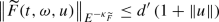 (3.3)
(3.3)for all \((t,\omega ,u)\in [0,T]\times \Omega \times E^c.\)
-
(6)
Let
 denote the space of \(\gamma \)-radonifying operators from H to
  for some constant
  , see, e.g., [35, Sec. 3.1]. Then the map
  is locally Lipschitz continuous in the sense that for all \(r>0\), there exists a constant \(L_{G}^{(r)}\) such that
for all \(\Vert u\Vert ,\Vert v\Vert \le r\) and \((t,\omega )\in [0,T]\times \Omega \). Moreover, for all \(u\in E^c\) and \(h\in H\) the map \((t,\omega )\mapsto G(t,\omega ,u)h\) is strongly measurable and adapted.
Finally, for some \(c'\ge 0\) we have
 (3.4)
(3.4)for all \((t,\omega ,u)\in [0,T]\times \Omega \times E^c.\)
 , the map
  is globally Lipschitz continuous in the third variable, uniformly with respect to the first and second variables. Moreover, for all
 denote the space of
  for some constant
  , see, e.g., [
 is locally Lipschitz continuous in the sense that for all

For a thorough discussion of UMD Banach spaces we refer to [13]. Banach spaces of type \(p\in [1,2]\) are treated in depth in [2, Sec. 6]. In particular, any \(L^p\)-space with \(p\in [2,\infty )\) has type 2. However, the space of continuous functions on any locally compact Hausdorff space is not a UMD space.
Remark 3.3
Assumptions 3.2(1)–(4) and (6) are—in the first 3 cases slightly modified versions of—Assumptions (A1), (A5), (A4), (F’) and (G’) in [35]. Assumption 3.2(5) is the assumption of [35, Prop. 3.8] on \(\widetilde{F}\). The main difference is that here the semigroup \(S^c\) is not necessarily strongly continuous on \(E^c\) but is analytic and that the embedding of \(E^{\theta }\hookrightarrow E^c\) is not necessarily dense.
Instead of (3.4) in Assumption 3.2(6), one may assume a slightly improved estimate

for some small \(\varepsilon >0\) depending on the parameters, as it is stated in (G’) of [35]. For simplicity, we chose not to include the small \(\varepsilon \) explicitly because to prove our main results it will not be needed.
We use that E is of type 2 in a crucial way e.g. in the first step of the proof of Theorem 3.6, (3.33) and (4.41), obtaining that the simple Lipschitz and growth conditions for the operator G in Assumption 3.2(6) suffice, see [56, Lem. 5.2].
Remark 3.4
In Assumptions 3.2(3), we use the fact that since S is analytic on E and by Assumptions 3.2(2), \(D(A)\subset E^{\theta }\hookrightarrow E^c\) holds, S leaves \(E^c\) invariant. Hence, the restriction \(S^c\) of S on \(E^c\) makes sense, and by assumption, \(S^c\) is an analytic contraction semigroup on \(E^c\). Using [1, Prop. 3.7.16], we obtain that this is equivalent to the fact that the generator \(A^c\) of \(S^c\) is sectorial and dissipative. Note that since \(S^c\) is not necessarily strongly continuous, \(A^c\) is not necessarily densely defined.
However, one can easily prove that \((A^c,D(A^c))\) is the part of (A, D(A)) in \(E^c\). By the definition of the generator (see [1, Def. 3.2.5]) we have that for \(\lambda >0\) and \(u\in E^c\)
By Assumptions 3.2(2), the last integral also converges in the norm of E. Thus,
The inclusion \(D(A)\subset E^c\) implies that in this case also \(R(\lambda ,A)u\in E^c\) is satisfied. Hence, we conclude that
Since \(\lambda >0\) and \(u\in E^c\) were arbitrary, the equality \((A^c,D(A^c))=(A|_{E^c}, D(A|_{E^c}))\) holds.
Recall that a mild solution of (SCP) is a solution of the following integral equation
where
denotes the “usual” convolution, and
denotes the stochastic convolution with respect to \(W_{H}.\) We also implicitly assume that all the terms on the right hand side of (3.5) are well-defined.
The following result is analogous to the statement of [35, Lem. 4.4] but with the semigroup \(S^c\) being an analytic contraction semigroup on \(E^c\) which is not necessarily strongly continuous. The main difference in the proof is the use of a different approximation argument as the one in [35] uses the strong continuity of \(S^c\) on \(E^c\) (the latter denoted by B there) in a crucial manner.
Lemma 3.5
Let \(S^c\) be an analytic contraction semigroup on \(E^c\). Let \(x\in E^c\) and \(F:[0,T]\times \Omega \times E^c\rightarrow E^c\) satisfy condition (4) of Assumptions 3.2, and denote by \(C:=\max \{a',b'\}\). Assume that \(u\in C((0,T];E^c)\cap L^{\infty }(0,T;E^c)\) and \(v\in C([0,T]\;E^c)\) satisfy
Then
Proof
Let \(A^c\) be the generator of \(S^c\), that is a sectorial and dissipative operator (see Remark 3.4) and fix \(v\in C([0,T]\;E^c)\) satisfying (3.6). Thus we can use methods from the proofs of [18, Prop. 6.2.2] and [19, Lem. 5.4]. Taking \(\lambda \in \rho (A^c)\), we introduce the problem on \(E^c\)
First take \(a=0\). Since \(x_{\lambda }\in D(A^c)\) and \(A^c\) is sectorial, by [39, Thm. 7.1.3(i)] this problem has a unique local mild solution in \(C([0,\delta ],E^c))\) for some \(\delta >0\), called \(u_{\lambda ,\delta }\), satisfying
for \(t\in [0,\delta ]\)
We now set \(a=\delta \) and take \(u_{\lambda ,\delta }(\delta )\) instead of \(x_{\lambda }\) in (3.8). Since \(u_{\lambda ,\delta }(\delta )\) satisfies (3.9) with \(t=\delta \) and \(S^c\) is analytic, we obtain that \(u_{\lambda ,\delta }(\delta )\) belongs to \(\overline{D(A^c)}\). Hence, by [39, Thm. 7.1.3(i)], there exists \(\varepsilon >0\) and a unique local mild solution of (3.8) in \(C([\delta ,\delta +\varepsilon ],E^c)\), called \(u_{\lambda ,\varepsilon }\), satisfying
Defining
yields a solution \(u_{\lambda ,\alpha }\in C([0,\alpha ],E^c)\) of (3.8) with \(a=0\) and \(\alpha =\delta +\varepsilon \). Again, \(u_{\lambda ,\alpha }(\alpha )\) can be taken as initial value for problem (3.8) with \(a=\alpha \), and the above procedure may be repeated indefinitely, up to construct a noncontinuable solution defined in a maximal time interval \(I(x_{\lambda })\). As in [39, Def. 7.1.7] we define by \(I(x_{\lambda })\) as the union of all the intervals \([0,\alpha ]\) such that (3.8) has a mild solution \(u_{\lambda ,\alpha }\) on this interval belonging to \(C([0,\alpha ],E^c)\). Denote by
and
which is well defined thanks to the uniqueness part of [39, Thm. 7.1.3(i)].
In the following, we first show that the desired norm estimate (3.7) holds for the maximal solution \(u_{\lambda ,\max }\) on \(I(x_{\lambda })\). At the end we will be able to prove that \(I(x_{\lambda })=[0,T]\).
Fix now \(t\in I(x_{\lambda })\). Then by definition, there exists \(\alpha >0\) such that \(t\in [0,\alpha ]\) and \(u_{\lambda ,\max }(t)= u_{\lambda ,\alpha }(t)\) holds for the mild solution \(u_{\lambda ,\alpha }\in C([0,\alpha ],E^c)\) of (3.8). For the sake of simplicity, we denote \(u_{\lambda }:=u_{\lambda ,\alpha }\).
Rewriting (3.9) for \(u_{\lambda }\) we obtain that for \(t\in [0,\alpha ]\)
where \(f_{\lambda }(s)=F(s,u_{\lambda }(s)+v(s)).\) Since \(f_{\lambda }\in C([0,\alpha ],E^c)\) and by definition, \(u_{\lambda }(0)=x_{\lambda }\in D(A^c)\) holds, we can apply [39, Prop. 4.1.8] and obtain that \(u_{\lambda }\) is a strong solution of (3.8) in the sense of [39, Def. 4.1.1]. This means, that there exists a sequence \((u_{\lambda ,n})\subset C^1([0,\alpha ],E^c)\cap C([0,\alpha ],D(A^c))\) such that
holds, as n goes to infinity. Using that \(u_{\lambda ,n}\in C^1([0,\alpha ],E^c)\), we have by [29, Thm. 17.9] that
Hence, for all \(u_{\lambda ,n}(t)^*\in \partial \Vert u_{\lambda ,n}(t)\Vert \),
Using the assumption on F, we obtain that
with
By Gronwall’s lemma from (3.11) we have
Observe that by the continuity of F and (3.10), we have that
Hence, letting \(n\rightarrow \infty \) in (3.12) and using (3.10) we obtain
Since \(A^c\) generates a contraction semigroup, \(\Vert x_{\lambda }\Vert \le \Vert x\Vert \) holds, and we obtain that
hence
Since \(t\in I(x_{\lambda })\) was arbitrary, and the right-hand-side of (3.13) does not depend on t, we have
Using [39, Prop. 7.1.8] (and its corollary) it follows that the solution \(u_{\lambda ,\max }\) is also global, hence \(I(x_{\lambda })=[0,T]\). Thus, (3.7) holds for \(u_{\lambda ,\max }\) and \(t\in [0,T]\).
Finally, arguing as in the last part of the proof of [18, Prop. 6.2.2], we obtain (3.7) for u(t). \(\square \)
Following [19], for a fixed \(T>0\) and \(q\ge 1\), we define the space
being a Banach space with norm
This Banach space will play a crucial role for the solutions of (SCP).
Theorem 3.6
Let \(T>0\), let \(2<q<\infty \) and suppose that Assumptions 3.2 hold with

Then for all \(\xi \in L^q(\Omega ,\mathscr {F}_0,\mathbb {P}; E^c)\) there exists a unique global mild solution \(X\in V_{T,q}\) of (SCP). Moreover, for some constant \(C_{q,T}>0\) we have
Proof
We only sketch a proof as it is analogous to the proofs of [35, Thm. 4.3] and [19, Thm. 5.3] with highlighting the necessary changes. We set
We argue in the same way as in the proof of [35, Prop. 3.8(1)] which uses implicitly that, according to Assumption 3.2(1), the Banach space E is of type 2, see also [56, p. 978]. The solution space will be \(V_{T,q}\) defined in (3.14) instead of \(L^q\left( \Omega ;C([0,T];E^c)\right) \) and \(F_n+\widetilde{F}\) instead of \(F_n\), we obtain that for each n there exists a mild solution \(X_n\in V_{T,q}\) of the problem (SCP) with \(F_n\) instead of F (see also the proof of [19, Thm. 5.3]). The mild solution \(X_n\) satisfies, for all \(t\in [0,T]\), the integral equation
almost surely.
We proceed in a completely analogous fashion as in the proof of [35, Thm. 4.3], with \(E^c\) instead of B. Instead of [35, Lem. 4.4] we use Lemma 3.5 with
and obtain that
Using that by Assumptions 3.2(2) \(E^{\theta }\hookrightarrow E^c\) holds, it follows from [56, Lem. 3.6] with \(\alpha =1\), \(\lambda =0\), \(\eta =\theta \),  that \(S*\widetilde{F}(\cdot ,X_n(\cdot ))\in C([0,T],E^c)\) is satisfied and

with \(C(T)\rightarrow 0\) if \(T\downarrow 0.\) Using (3.3) and proceeding as in the proof of [35, Thm. 4.3], we obtain that for each \(T>0\) there exists a constant \(C_{q,T}>0\) such that
We remark that the estimates needed use only the continuity of the embedding \(E^{\theta }\hookrightarrow E^c.\) Once (3.18) has been established we can conclude, the same way as in the proof of [19, Thm. 5.3] the existence and uniqueness of a process \(X\in L^q\left( \Omega ;L^\infty (0,T;E^c\right) )\) with
such that for \(t\in [0;T]\),
almost surely, and thus, X is the unique mild solution of (SCP) in \(L^q\left( \Omega ;L^\infty (0,T;E^c\right) )\).
To prove the continuity of the trajectories of X we first note that the analyticity of S on \(E^c\) immediately implies that \((0,T]\ni t\rightarrow S(t)\xi \in E^c\) is continuous. Next, we use [39, Pro. 4.2.1] and the continuity of F to obtain that
is continuous. Using [56, Lem. 3.6] as above, we obtain that \(S*\widetilde{F}(\cdot ,X(\cdot ))\in C([0,T],E^c)\) holds. Applying analogous estimates as in the proof of [35, Thm. 4.3], we may conclude that there exists \(C(T)>0\) such that
Hence, it follows that
is continuous almost surely. Thus, by (3.20) and the already established fact that \(X\in L^q\left( \Omega ;L^\infty (0,T;E^c\right) )\), we obtain that \(X\in V_{T,q}\) and by (3.19) the estimate (3.15) holds. \(\square \)
For our next result, introduce the following set of assumptions on the operators in (SCP).
Assumptions 3.7
-
(1)
Let E be a UMD Banach space of type 2 and (A, D(A)) a densely defined, closed and sectorial operator on E.
-
(2)
We have continuous (but not necessarily dense) embeddings for some \(\theta \in (0,1)\)
$$E^{\theta }\hookrightarrow E^c\hookrightarrow E.$$ -
(3)
The strongly continuous analytic semigroup S generated by (A, D(A)) on E restricts to an analytic, contractive semigroup, denoted by \(S^{c}\) on \(E^c\), with generator \((A^c,D(A^c))\).
-
(4)
The map \(F:[0,T]\times \Omega \times E^c\rightarrow E^c\) is continuous in the first variable and locally Lipschitz continuous in the third variable in the sense that for all \(r>0\), there exists a constant \(L_{F}^{(r)}\) such that
$$\begin{aligned} \left\| F(t,\omega ,u)-F(t,\omega ,v)\right\| \le L_{F}^{(r)}\Vert u-v\Vert \end{aligned}$$for all \(\Vert u\Vert ,\Vert v\Vert \le r\) and \((t,\omega )\in [0,T]\times \Omega \) and there exists a constant \(C_{F,0}\ge 0\) such that
$$\begin{aligned} \left\| F(t,\omega ,0)\right\| \le C_{F,0},\quad t\in [0,T],\; \omega \in \Omega . \end{aligned}$$Moreover, for all \(u\in E^c\) the map \((t,\omega )\mapsto F(t,\omega ,u)\) is strongly measurable and adapted.
Finally, for suitable constants \(a',b'\ge 0\) and \(N\ge 1\) we have
$$\begin{aligned} \langle A u+F (t,u+v), u^*\rangle \le a'(1+\Vert v\Vert )^N+b'\Vert u\Vert \end{aligned}$$for all \(u\in D(A|_{E^c})\), \(v\in E^c\) and \(u^*\in \partial \Vert u\Vert ,\) see (3.2).
-
(5)
There exist constants \(a'',\, b'',\, k,\, K>0\) with \(K\ge k\) such that the function \(F:[0,T]\times \Omega \times E^c\rightarrow E^c\) satisfies
$$\begin{aligned} \langle F (t,\omega , u+v)-F (t,\omega , v), u^*\rangle \le a''(1+\Vert v\Vert )^K-b''\Vert u\Vert ^k \end{aligned}$$(3.21)for all \(t\in [0,T]\), \(\omega \in \Omega \), \(u,v\in E^c\) and \(u^*\in \partial \Vert u\Vert ,\) and
$$\begin{aligned} \left\| F(t,v)\right\| \le a''(1+\Vert v\Vert )^K \end{aligned}$$for all \(v\in E^c.\)
-
(6)
For some constant
 , the map
  is globally Lipschitz continuous in the third variable, uniformly with respect to the first and second variables. Moreover, for all \(u\in E^c\) the map \((t,\omega )\mapsto \widetilde{F}(t,\omega ,u)\) is strongly measurable and adapted.
Finally, for some \(d'\ge 0\) we have
 (3.22)
for all \((t,\omega ,u)\in [0,T]\times \Omega \times E^c.\)
-
(7)
Let
 denote the space of \(\gamma \)-radonifying operators from H to
  for some
  , see, e.g., [35, Sec. 3.1]. Then the map
  is locally Lipschitz continuous in the sense that for all \(r>0\), there exists a constant \(L_{G}^{(r)}\) such that
for all \(\Vert u\Vert ,\Vert v\Vert \le r\) and \((t,\omega )\in [0,T]\times \Omega \). Moreover, for all \(u\in E^c\) and \(h\in H\) the map \((t,\omega )\mapsto G(t,\omega ,u)h\) is strongly measurable and adapted.
Finally, for suitable constant \(c',\)

for all \((t,\omega ,u)\in [0,T]\times \Omega \times E^c.\)
 , the map
  is globally Lipschitz continuous in the third variable, uniformly with respect to the first and second variables. Moreover, for all
 denote the space of
  for some
  , see, e.g., [
 is locally Lipschitz continuous in the sense that for all

Remark 3.8
Assumptions 3.7(1)–(5) and (7) are—in the first 3 cases slightly modified versions of—Assumptions (A1), (A5), (A4), (F’) and (G’) in [35]. Assumption (6) is the assumption of [35, Prop. 3.8] on \(\widetilde{F}\). The main difference, besides the lack of strong continuity of S on \(E^c\) and that the embedding \(E^{\theta }\hookrightarrow E^c\) is not necessarily dense, is that instead of (F”) we impose a possibly asymmetric growth condition (3.21) on F. This is necessary so that later when we apply the abstract theory to (1.1) we may consider polynomial reaction terms with different degrees on different edges of the graph. The growth condition on G in Assumption 3.7(7) is also different from the linear growth condition on G in (G”) of [35] as it reflects the possibly asymmetric growth condition on F. It becomes a linear growth condition when \(k=K\).
The following result is analogous to the statement of [35, Lem. 4.8] but with the semigroup \(S^c\) being an analytic contraction semigroup on \(E^c\) which is not necessarily strongly continuous and with the asymmetric growth condition (3.21) on F. Again, the main difference in the proof is the use of a different approximation argument as the Yosida approximation argument in [35] uses the strong continuity of \(S^c\) on \(E^c\) (the latter denoted by B there) in a crucial manner.
Lemma 3.9
Let \(S^c\) be an analytic contraction semigroup on \(E^c\). Let \(x\in E^c\) and \(F:[0,T]\times \Omega \times E^c\rightarrow E^c\) satisfy condition (4) and (5) of Assumptions 3.7. Assume that \(u\in C((0,T];E^c)\cap L^{\infty }(0,T;E^c)\) and \(v\in C([0,T]\;E^c)\) satisfy
Then
with \(c=\left( \frac{4a''}{b''}\right) ^{\frac{1}{k}}.\)
Proof
We will proceed similarly as in Lemma 3.5. We denote by \(A^c\) the generator of \(S^c\), being sectorial and dissipative (see Remark 3.4) and fix \(v\in C([0,T]\;E^c)\) satisfying (3.23). Hence, we can take \(\lambda \in \rho (A^c)\), and introduce the problem on \(E^c\)
As we have showed in the proof of Lemma 3.5, there exists a unique global solution \(u_{\lambda }\in C([0,T],E^c))\) of (3.25), satisfying
where \(f_{\lambda }(s)=F(s,u_{\lambda }(s)+v(s)).\) Since \(f_{\lambda }\in C([0,T],E^c)\) and by definition, \(u_{\lambda }(0)=x_{\lambda }\in D(A^c)\) holds, we can apply [39, Prop. 4.1.8] and obtain that \(u_{\lambda }\) is a strong solution of (3.25) in the sense of [39, Def. 4.1.1]. This means, that there exists a sequence \((u_{\lambda ,n})\subset C^1([0,T],E^c)\cap C([0,T],D(A^c))\) such that
holds, as n goes to infinity. Using that \(u_{\lambda ,n}\in C^1([0,T],E^c)\), we have by [29, Thm. 17.9] that
Hence, for all \(u_{\lambda ,n}(t)^*\in \partial \Vert u_{\lambda ,n}(t)\Vert \),
Using now the dissipativity of \(A^c\) (see Remark 3.4) and the assumptions on F, we obtain that
with
By the continuity of F and (3.26), we have that
We now fix \(n\in \mathbb {N}\) and define \(\varphi (t):=\Vert u_{\lambda ,n}(t)\Vert \) and
Then \(\varphi \) is absolutely continuous and by (3.27)
holds almost everywhere. We will prove that
where \(x_{\varphi }=u_{\lambda ,n}(0)\). Assume to the contrary that for some \(t_0\in [0,T]\)
Since \(\varphi (0)=\Vert x_{\varphi }\Vert \), we have that \(t_0\in (0,T]\). Let \(\psi :I\rightarrow \mathbb {R}\) be the unique maximal solution of
We can use [35, Cor. 4.7] with \(u^+(t)=\psi (t)\), \(u^-(t)=\varphi (t)\),
and the assumption \(u^+(t_0)+\Vert x_{\varphi }\Vert \le u^-(t_0)\). This implies that \(u^+(t)+\Vert x_{\varphi }\Vert \le u^-(t)\), that is,
Using the same arguments as in the proof of [35, Lem. 4.8] we obtain that \(0\in I\) and
This implies by the definition of \(\psi \) that \(\psi '(t)<0\); hence, \(\psi \) is decreasing. Combining this together with (3.31) and (3.30) it follows that
hence
which is a contradiction.
Thus, we have proved (3.29). Since n was arbitrary, we obtain that for all \(n\in \mathbb {N}\)
Letting \(n\rightarrow \infty \), by (3.26) and (3.28) we conclude that
Finally, using the same argument as at the end of the proof of [18, Prop. 6.2.2], we obtain that for any t, the net \(\{u_{\lambda }(t)\}_{\lambda \in \rho (A^c)}\) is a Cauchy-net in \(E^c\); hence, it is convergent and the limit is u(t). This yields (3.24). \(\square \)
The next result is a generalized version of that of Kunze and van Neerven which was first proved in [35, Thm. 4.9] but with a typo in the statement and was later corrected in the recent arXiv preprint [36, Thm. 4.9].
Theorem 3.10
Let \(T>0\), \(2<q<\infty \) and suppose that Assumptions 3.7 hold with

Then for all \(\xi \in L^q(\Omega ,\mathscr {F}_0,\mathbb {P}; E^c)\) there exists a global mild solution \(X\in V_{T,q}\) of (SCP). Moreover, for some constant \(C_{q,T}>0\) we have
Proof
We can proceed similarly as in the proofs of [35, Thm. 4.9] and [19, Thm. 5.9]. We set
We obtain by Theorem 3.6 that for each n there exists a global mild solution \(X_n\in V_{T,q}\) of the problem (SCP) with \(G_n\) instead of G (see also the proof of [19, Thm. 5.5]). Using (3.16) and setting
we obtain that

where \(\lesssim \) denotes that the expression on the left-hand-side is less or equal to a constant times the expression on the right-hand-side. In the last inequality we have used estimate (3.17) with \(C(T)\rightarrow 0\) if \(T\downarrow 0\) and Lemma 3.9 with \(u=u_n\) and \(v=v_n\).
As in the proof of [35, Thm. 4.3] with \(E^c\) instead of B, we obtain that for each \(T>0\) there exist a constant \(C'_{T}>0\) such that

where in the second inequality we have used Assumptions 3.7(7) and we have \(C'(T)\rightarrow 0\) when \(T\downarrow 0\). Combining this with (3.22) and (3.32) we obtain that there are positive constants \(C_0\), \(C_1\) and \(C_2(T)\) such that
with \(C_2(T)\rightarrow 0\) as \(T\downarrow 0.\) The proof can be finished as that of Theorem 3.6. \(\square \)
4 A stochastic reaction–diffusion equation
4.1 Preparatory results
In order to apply the abstract result of Theorem 3.10 to the stochastic reaction–diffusion equation, we need to prove some preliminary results regarding the setting of Sect. 2. We make use of the fact that the semigroups involved here all leave the corresponding real spaces invariant (this follows from the first bullet in the proof of Lemma B.1 and the corresponding Beurling–Deny criterion).
Definition 4.1
We denote by
the product space of continuous functions on the edges (not necessarily continuous in the vertices) and denote its elements by
The norm is defined as usual with
This space will play the role of the space \(E^c\) in our setting. We recall that for \(p\in [1,\infty ]\) the operators \((\mathcal {A}_p,D(\mathcal {A}_p))\) are generators of analytic semigroups (see Proposition 2.4) on the spaces \(\mathcal {E}_p\) defined in (2.15).

We will need the following result on the fractional power spaces \(\mathcal {E}_p^{\theta }.\)
Lemma 4.2
For the fractional domain spaces \(\mathcal {E}_p^{\theta }\) defined in (4.1) and \(1< p<\infty \) arbitrary, we have that
-
(1)
if \(0<\theta < \frac{1}{2p}\), then
$$\begin{aligned} \mathcal {E}_p^{\theta }\cong \left( \prod _{j=1}^m W^{2\theta ,p}(0,1;\mu _j \mathrm{d}x)\right) \times \mathbb {R}^n; \end{aligned}$$ -
(2)
if \(\theta > \frac{1}{2p}\), then
$$\begin{aligned} \mathcal {E}_p^{\theta } \cong \left( \prod _{j=1}^m W_{0}^{2\theta ,p}(0,1;\mu _j \mathrm{d}x)\right) \times \mathbb {R}^n. \end{aligned}$$
Proof
By Proposition 2.4, the operator \((\mathcal {A}_p,D(\mathcal {A}_p))\) generates a positive, contraction semigroup on \(\mathcal {E}_p\). Hence, we can use [7, Thm. in \(\mathsection \)4.7.3] (see also [25]) obtaining that for any \(\omega '>0\), \(\omega '-\mathcal {A}_p\) has a bounded \(H^{\infty }(\Sigma _{\varphi })\)-calculus for each \(\varphi >\frac{\pi }{2}\). Proposition 2.4 implies that \(\omega '-\mathcal {A}_p\) is injective and sectorial; thus, it has bounded imaginary powers (BIP). Therefore, by [7, Prop. in \(\mathsection \)4.4.10] (see also [40, Thm. 11.6.1]), it follows that for the complex interpolation spaces
holds with equivalence of norms. Denote
where \(W_{0}^{2,p}(0,1;\mu _j \mathrm{d}x)=W^{2,p}(0,1;\mu _j \mathrm{d}x)\cap W_{0}^{1,p}(0,1;\mu _j \mathrm{d}x),\) \(j=1,\dots , m.\) Hence, \(W_0(G)\) contains such vectors of functions that are twice weakly differentiable on each edge and continuous in the vertices with Dirichlet boundary conditions. By [45, Cor. 3.6],
where the isomorphism is established by a similarity transform of \(\mathcal {E}_p\). Using general interpolation theory, see e.g. [50, Sec. 4.3.3], we have that if \(\theta < \frac{1}{2p}\), then
Hence, summing up (4.2), (4.3) and (4.4), for \(\theta < \frac{1}{2p}\)
holds.
Furthermore, using again [50, Sec. 4.3.3], for \(\theta >\frac{1}{2p}\) we have that
Hence, by (4.2), (4.3) and (4.5), for \(\theta >\frac{1}{2p}\)
holds. \(\square \)
Corollary 4.3
For \(\theta > \frac{1}{2p}\) the following continuous embeddings are satisfied:
Proof
According to Lemma 4.2(2) we have that for \(\theta > \frac{1}{2p}\)
holds. Hence, by Sobolev imbedding we obtain that for \(\theta >\frac{1}{2p}\)
is satisfied. The claim follows by observing that \(\mathcal {E}^c\hookrightarrow \mathcal {E}_p\). \(\square \)
In the following, we will prove that each of the semigroups \((\mathcal {T}_p(t))_{t\ge 0}\) restricts to the same analytic semigroup of contractions on \(\mathcal {E}^c\).
Proposition 4.4
For all \(p\in [1,\infty ]\), the semigroups \(\mathcal {T}_p\) leave \(\mathcal {E}^c\) invariant, and the restrictions \(\mathcal {T}_p|_{\mathcal {E}^c}\) all coincide that we denote by \(\mathcal {S}^c\). The semigroup \(\mathcal {S}^c\) is analytic and contractive on \(\mathcal {E}^c\). Its generator \((\mathcal {A}^c,D(\mathcal {A}^c))\) coincides with the part \((\mathcal {A}_p|_{\mathcal {E}^c},D(\mathcal {A}_p|_{\mathcal {E}^c}))\) of the operator \((\mathcal {A}_p,D(\mathcal {A}_p))\) in \(\mathcal {E}^c\) for any \(p\in [1,\infty ]\).
Proof
First we will show that for each \(p\in [1,\infty ]\), \(D(\mathcal {A}_p)\subset \mathcal {E}^c\) holds. If \(p\in [1,\infty )\) it follows easily from (2.17) and Sobolev imbedding. For \(p=\infty \) take \(U\in D(\mathcal {A}_{\infty })\). Then for any \(\lambda >0\) there exists \(V\in \mathcal {E}_{\infty }\) such that \(R(\lambda ,\mathcal {A}_{\infty })V=U\). Using that the semigroup \(\mathcal {T}_2\) is the extension of \(\mathcal {T}_{\infty }\) to \(\mathcal {E}_2\) by (2.16) and \(\mathcal {E}_{\infty }\hookrightarrow \mathcal {E}_2\) holds, by a similar argument as in Remark 3.4 we obtain that \(V\in \mathcal {E}_2\) and \(R(\lambda ,\mathcal {A}_{2})V=U\in D(\mathcal {A}_2)\). The claim follows now by observing \(D(\mathcal {A}_2)\subset \mathcal {E}^c\).
From Proposition 2.4, we know that for each \(p\in [1,\infty ]\) the semigroup \(\mathcal {T}_p\) is analytic and contractive. Hence, using the inclusion \(D(\mathcal {A}_p)\subset \mathcal {E}^c\) and [1, Thm. 3.7.19], we obtain that \(\mathcal {T}_p\) leaves \(\mathcal {E}^c\) invariant. By (2.16), we also have that the restrictions on \(\mathcal {E}^c\) all coincide; thus, we may use \(\mathcal {S}^c\) to denote this common restriction. It is straightforward that \(\mathcal {S}^c\) is a contraction semigroup on \(\mathcal {E}^c\) since \(\mathcal {T}_{\infty }\) is a contraction semigroup on \(\mathcal {E}_{\infty }\) and the norms on \(\mathcal {E}^c\) and \(\mathcal {E}_{\infty }\) coincide.
Using the same argument as in Remark 3.4, and the fact \(D(\mathcal {A}_p)\subset \mathcal {E}^c\), we obtain that \(\mathcal {A}^c=\mathcal {A}_p|_{\mathcal {E}^c}\) for all \(p\in [1,\infty ]\).
It remains to prove that \(\mathcal {S}^c\) is analytic. We now use that \(\mathcal {T}_{\infty }\) is analytic on \(\mathcal {E}_{\infty }\). That is, by [1, Cor. 3.7.18], there exists \(r>0\) such that \(\left\{ is:s\in \mathbb {R},\; |s|>r\right\} \subset \rho (\mathcal {A}_{\infty })\) and
Since \(\mathcal {A}_{\infty }|_{\mathcal {E}^c}=\mathcal {A}^c\), the analogue of (4.6) also holds with \(\mathcal {A}^c\) instead of \(\mathcal {A}_{\infty }\) and with respect to the norm of \(\mathcal {E}^c\). Hence, using [1, Cor. 3.7.18] again, we obtain that the semigroup \(\mathcal {S}^c\) generated by \(\mathcal {A}^c\) on \(\mathcal {E}^c\) is analytic. \(\square \)
4.2 Main results
We now apply the results of the previous sections to the following stochastic evolution equation, based on (2.2) (see [11, Sec. 2], [35, Sec. 5]). We prescribe stochastic noise in the nodes as well as on the edges of the network.
Let \((\Omega ,\mathscr {F},\mathbb {P})\) be a complete probability space endowed with a right-continuous filtration \(\mathbb {F}=(\mathscr {F}_t)_{t\in [0,T]}\) for some \(T>0\) given. We consider the problem
Here \(\dot{\beta }_i(t)\), \(i=1,\dots ,n\), are independent noises; written as formal derivatives of independent scalar Brownian motions \((\beta _i(t))_{t\in [0,T]}\), defined on \((\Omega ,\mathscr {F},\mathbb {P})\) with respect to the filtration \(\mathbb {F}\). The terms \(\frac{\partial w_j}{\partial t}\), \(j=1,\dots ,m\), are independent space-time white noises on [0, 1]; written as formal derivatives of independent cylindrical Wiener processes \((w_j(t))_{t\in [0,T]}\), defined on \((\Omega ,\mathscr {F},\mathbb {P})\), in the Hilbert space \(L^2(0,1; \mu _j \mathrm{d}x)\) with respect to the filtration \(\mathbb {F}\).
In contrast to Sect. 2, we add a first order term \(d_j(x)\cdot u_j'(t,x)\) to the first equation of (2.2) assuming
The functions \(f_j:[0,T]\times \Omega \times [0,1]\times \mathbb {R}\rightarrow \mathbb {R}\) are polynomials of the form
for some integers \(k_j,\) \(j=1,\dots ,m.\) For the coefficients we assume that there are constants \(0<c\le C<\infty \) such that
for all \((t,\omega ,x)\in [0,T]\times \Omega \times [0,1]\), see [35, Ex. 4.2]. Furthermore, we suppose that
and that the coefficients \(a_{j,l}:[0,T]\times \Omega \times [0,1]\rightarrow \mathbb {R}\) are jointly measurable and adapted in the sense that for each j and l and for each \(t\in [0,T]\), the function \(a_{j,l}(t,\cdot )\) is \(\mathscr {F}_t\otimes \mathcal {B}_{[0,1]}\)-measurable, where \(\mathcal {B}_{[0,1]}\) denotes the sigma-algebra of the Borel sets on [0, 1].
Remark 4.5
The functions coming from the classical FitzHugh–Nagumo problem (see, e.g., [11])
with \(a_j\in (0,1)\) satisfy the conditions above.
Furthermore, let
For the functions \(g_i\) we assume
where the constants k and K are defined in (4.9). We further require that the functions \(g_i\) are jointly measurable and adapted in the sense that for each i and \(t\in [0,T]\), \(g_i(t,\cdot )\) is \(\mathscr {F}_t\otimes \mathcal {B}_{\mathbb {R}}\)-measurable, where \(\mathcal {B}_{\mathbb {R}}\) denotes the sigma-algebra of the Borel sets on \(\mathbb {R}\).
We suppose that
We further assume that the functions \(h_j\) are jointly measurable and adapted in the sense that for each j and \(t\in [0,T]\), \(h_j(t,\cdot )\) is \(\mathscr {F}_t\otimes \mathcal {B}_{[0,1]}\otimes \mathcal {B}_{\mathbb {R}}\)-measurable, where \(\mathcal {B}_{[0,1]}\) and \(\mathcal {B}_{\mathbb {R}}\) denote the sigma-algebras of the Borel sets on [0, 1] and \(\mathbb {R}\), respectively.
We rewrite system (4.7) in an abstract form analogously to (SCP)
The operator \((\mathcal {A}, D(\mathcal {A}))\) is \((\mathcal {A}_p, D(\mathcal {A}_p))\) for some large \(p\in [2,\infty )\), where p will be chosen in (4.22), (4.25) and (4.35), (4.43) later. Hence, by Proposition 2.4, \(\mathcal {A}\) is the generator of the strongly continuous analytic semigroup \(\mathcal {S}:=\mathcal {T}_p(t)\) on the Banach space \(\mathcal {E}_p\), and \(\mathcal {E}_p\) is a UMD space of type 2.
For the function \(\mathcal {F}:[0,T]\times \Omega \times \mathcal {E}^c\rightarrow \mathcal {E}^c\) we have
with
\(t\in [0,T]\), \(\omega \in \Omega \).
We now define \(\widetilde{\mathcal {F}}\) and \(\mathcal {G}\) and after that we prove that they map between the appropriate spaces as assumed in Sect. 3. Let
be defined as a map from \((C^1[0,1])^m\times \mathbb {R}^n\) to \(\mathcal {E}_p\) for any \(p>1\) with
To define the operator \(\mathcal {G}\), we argue in analogy with [36, Sec. 5]. First define
the product \(L^2\)-space, see (2.9), which is a Hilbert space. We further define the multiplication operator \(\Gamma :[0,T]\times \Omega \times \mathcal {E}^c\rightarrow \mathcal {L}(\mathcal {H})\) as
for \(U=\begin{pmatrix} u \\ r \end{pmatrix}\in \mathcal {E}^c\) and \(Y\in \mathcal {H}\) with
and
Because of the assumptions on the functions \(h_j\) and \(g_i\), \(\Gamma \) clearly maps into \(\mathcal {L}(\mathcal {H}).\)
Let \((\mathcal {A}_2,D(\mathcal {A}_2))\) be the generator on \(\mathcal {H}=\mathcal {E}_2,\) see Proposition 2.4, and pick  . Using Lemma 4.2(2) we have that there is an isomorphism

By Corollary 4.3, \(\mathcal {H}_1 \hookrightarrow \mathcal {E}^c\) holds. Using Corollary 4.3 again, we have that the there exists a continuous embedding
for \(p\ge 2\) arbitrary.
Let \(\nu >0\) arbitrary and define now \(\mathcal {G}\) by

Lemma 4.6
-
1.
Let \(p>1\) arbitrary. Then the mapping defined in (4.15) can be extended to a linear and continuous operator from \(\mathcal {E}^c\) into \(\mathcal {E}_p^{-\frac{1}{2}}\), that we also call \(\widetilde{\mathcal {F}}\).
-
2.
Let \(p\ge 2\) and
 be arbitrary. The operator \(\mathcal {G}\) defined in (4.18) maps \([0,T]\times \Omega \times \mathcal {E}^c\) into \(\gamma (\mathcal {H},\mathcal {E}_p^{-\kappa _{G}})\).
 be arbitrary. The operator
 Proof
-
1.
To prove the claim for \(\widetilde{\mathcal {F}}\) let \(p> 1\) arbitrary and \(q:=(1-\frac{1}{p})^{-1}\). We first investigate the operator \(\widetilde{\mathcal {F}}_1\) defined in (4.16) and take \(u\in (C^1[0,1])^m\), \(v\in (W_0^{1,q}(0,1))^m\) obtaining that for a constant \(c'>0\)
$$\begin{aligned} \left| \langle \widetilde{\mathcal {F}}_1 u, v\rangle \right|&=\left| \sum _{j=1}^m\int _0^1 d_j(x)u_j'(x)v_j(x)\, \mathrm{d}x\right| =\left| -\sum _{j=1}^m\int _0^1 u_j(x)(d_jv_j)'(x)\, \mathrm{d}x\right| \\&\le c'\cdot \Vert u\Vert _{(C[0,1])^m}\cdot \Vert d\Vert _{(W^{1,\infty }(0,1))^m}\cdot \Vert v\Vert _{(W_0^{1,q}(0,1))^m} \end{aligned}$$where \(d=(d_1,\dots ,d_m)\) and \(\langle \cdot ,\cdot \rangle \) denotes the duality of \((W_0^{1,q}(0,1))^m\). Hence, for a positive constant c,
$$\begin{aligned} \frac{\left| \langle \widetilde{\mathcal {F}}_1u, v\rangle \right| }{\Vert v\Vert _{(W_0^{1,q}(0,1))^m}}\le c\Vert u\Vert _{(C[0,1])^m}. \end{aligned}$$Since \((C^1[0,1])^m\) is dense in \((C[0,1])^m\), \(\widetilde{\mathcal {F}}_1\) can be extended to a continuous linear operator
$$\begin{aligned} \widetilde{\mathcal {F}}_1:(C[0,1])^m \rightarrow \left( (W_0^{1,q}(0,1))^m\right) ^* \end{aligned}$$with
$$\begin{aligned} \Vert \widetilde{\mathcal {F}}_1 u\Vert _{\left( (W_0^{1,q}(0,1))^m\right) ^*}\le c\Vert u\Vert _{(C[0,1])^m},\quad u\in (C[0,1])^m. \end{aligned}$$(4.19)By [55, Thm. 3.1.4] we have
$$\begin{aligned} \left( \mathcal {E}_q^{\frac{1}{2}}\right) ^*\cong \mathcal {E}_p^{-\frac{1}{2}}\;\text { for }\frac{1}{p}+\frac{1}{q}=1. \end{aligned}$$Lemma 4.2 implies that
$$\begin{aligned} \mathcal {E}_q^{\frac{1}{2}} \cong \left( \prod _{j=1}^m W_{0}^{1,q}(0,1;\mu _j \mathrm{d}x)\right) \times \mathbb {R}^n\cong (W_0^{1,q}(0,1))^m\times \mathbb {R}^n \end{aligned}$$holds, hence
$$\begin{aligned} \mathcal {E}_p^{-\frac{1}{2}}\cong \left( \mathcal {E}_q^{\frac{1}{2}}\right) ^*\cong \left( (W_0^{1,q}(0,1))^m\right) ^*\times \mathbb {R}^n. \end{aligned}$$By definition (4.15) of \(\widetilde{\mathcal {F}}\) and by the extension (4.19) of \(\widetilde{\mathcal {F}}_1\) this means exactly that \(\widetilde{\mathcal {F}}\) can be extended to a continuous linear operator from \(\mathcal {E}^c\) to \(\mathcal {E}_p^{-\frac{1}{2}}\) with
$$\begin{aligned} \Vert \widetilde{\mathcal {F}} U\Vert _{\mathcal {E}_p^{-\frac{1}{2}}}\le c\Vert U\Vert _{\mathcal {E}^c},\quad U\in \mathcal {E}^c. \end{aligned}$$(4.20) -
2.
We can argue as in [56, Sec. 10.2]. Using [56, Lem. 2.1(4)], we obtain in a similar way as in [56, Cor. 2.2]) that \(\jmath \in \gamma (\mathcal {H}_1,\mathcal {E}_p)\), since
 holds. Hence, by the definition of \(\mathcal {G}\) and the ideal property of \(\gamma \)-radonifying operators, the mapping \(\mathcal {G}\) takes values in \(\gamma (\mathcal {H},\mathcal {E}_p^{-\kappa _{G}})\).
 holds. Hence, by the definition of
 \(\square \)
The driving noise process \(\mathcal {W}\) is defined by
and thus, \((\mathcal {W}(t))_{t\in [0,T]}\) is a cylindrical Wiener process, defined on \((\Omega ,\mathscr {F},\mathbb {P})\), in the Hilbert space \(\mathcal {H}\) with respect to the filtration \(\mathbb {F}\).
Similarly to (3.14) for a fixed \(T>0\) and \(q\ge 1\) we define the space
being a Banach space with norm
This Banach space will play a crucial role for the solutions of (SCPn).
We will state now the result regarding system (SCPn).
Theorem 4.7
Let \(\mathcal {F}\), \(\widetilde{\mathcal {F}}\), \(\mathcal {G}\) and \(\mathcal {W}\) defined as in (4.14), (4.15), (4.18) and (4.21), respectively. Let \(q>4\) be arbitrary. Then for every \(\xi \in L^q(\Omega ,\mathscr {F}_0,\mathbb {P};\mathcal {E}^c)\) equation (SCPn) has a unique global mild solution in \(\mathcal {V}_{T,q}\).
Proof
The condition \(q > 4\) allows us to choose \(2 \le p < \infty \), \(\theta \in (0,\frac{1}{2})\) and  such that
and

We will apply Theorem 3.10 with \(\theta \) and  having the properties above. To this end we have to check Assumptions 3.7 for the mappings in (SCPn), taking \(\mathcal {A}=\mathcal {A}_p\) for the p chosen above.
-
(a)
Assumption (1) is satisfied because of the generator property of \(\mathcal {A}_p\), see Proposition 2.4.
-
(b)
Assumption (2) is satisfied since (4.22) holds and we can use Corollary 4.3.
-
(c)
Assumption (3) is satisfied because of Proposition 4.4.
-
(d)
To satisfy Assumptions (4) and (5) we first remark that the locally Lipschitz continuity of \(\mathcal {F}\) follows from (4.8). In the following, we have to consider vectors \(U^*\in \partial \Vert U\Vert \) for \(U=\left( {\begin{matrix}u\\ r\end{matrix}}\right) \in \mathcal {E}^c\). It is easy to see that there exists \(U^*\in \partial \Vert U\Vert \) of the form
$$\begin{aligned} U^*=\left( {\begin{matrix}u^*\\ r^*\end{matrix}}\right) \end{aligned}$$with
$$\begin{aligned} u^*\in \partial \Vert u\Vert _{(C[0,1])^m}\text { and }r^*\in \partial \Vert r\Vert _{\ell ^{\infty }}. \end{aligned}$$Using that the functions \(f_j\) are polynomials of the 4th variable (see (4.8)), a similar computation as in [35, Ex. 4.2] shows that for all \(j=1,\dots ,m,\) and for a suitable constant \(a'\ge 0\)
$$\begin{aligned} f_j(t,\omega ,x,\eta +\zeta )\cdot {{\,\mathrm{sgn}\,}}\eta \le a'(1+|\zeta |^{2k_j+1}) \end{aligned}$$holds. Using techniques from [23, Sec. 4.3] we obtain that
$$\begin{aligned} \langle \mathcal {A}U+\mathcal {F}(t,U+V), U^*\rangle \le a'(1+\Vert V\Vert _{\mathcal {E}^c})^K+b'\Vert U\Vert _{\mathcal {E}^c} \end{aligned}$$with K defined in (4.9) and for all \(U\in D(\mathcal {A}_p|_{\mathcal {E}^c})\), \(V\in \mathcal {E}^c\) and \(U^*\in \partial \Vert U\Vert .\) Following the computation of [35, Ex. 4.5], we obtain that for suitable positive constants a, b, c and for all \((t,\omega ,x)\in [0,T]\times \Omega \times [0,1]\) and \(j=1,\dots ,m\),
$$\begin{aligned} \left[ f_j(t,\omega ,x,\eta +\zeta )-f_j(t,\omega ,x,\zeta )\right] \cdot {{\,\mathrm{sgn}\,}}\eta \le a-b|\eta |^{2k_j+1}+c|\zeta |^{2k_j+1} \end{aligned}$$holds. Using again techniques from [23, Sec. 4.3] (see also [19, Rem. 5.1.2 and (5.19)], we obtain that for k and K defined in (4.9) \(K\ge k\) holds and
$$\begin{aligned} \langle \mathcal {F}(t,\omega , U+V)-\mathcal {F}(t,\omega , V), U^*\rangle \le a''(1+\Vert V\Vert _{\mathcal {E}^c})^K-b''\Vert U\Vert _{\mathcal {E}^c}^k \end{aligned}$$for all \(t\in [0,T]\), \(\omega \in \Omega \), \(U,V\in \mathcal {E}^c\) and \(U^*\in \partial \Vert U\Vert .\) Furthermore,
$$\begin{aligned} \left\| \mathcal {F}(t,V)\right\| _{\mathcal {E}^c}\le a''(1+\Vert V\Vert _{\mathcal {E}^c})^K \end{aligned}$$(4.23)for all \(V\in \mathcal {E}^c.\)
-
(e)
To check Assumption (6) we refer to Lemma 4.6. This implies that
 with
with  . Since \(\widetilde{F}\) is a continuous linear operator, the rest of the statement also follows.
 -
(f)
To check Assumption (7) note that by Lemma 4.6, \(\mathcal {G}\) takes values in \(\gamma (\mathcal {H},\mathcal {E}_p^{-\kappa _{G}})\) with \(\mathcal {H}=\mathcal {E}_2\) and
 chosen above. We apply a similar computation as in the proof of [56, Thm. 10.2]. We fix \(U,V\in \mathcal {E}^c\) and let $$\begin{aligned} R:=\max \left\{ \Vert U\Vert _{\mathcal {E}^c},\Vert V\Vert _{\mathcal {E}^c}\right\} . \end{aligned}$$
Furthermore, we denote the matrix from (4.17) by
$$\begin{aligned} \mathcal {M}_{\Gamma }(t,\omega ,U):=\begin{pmatrix} \Gamma _1(t,\omega ,\cdot ,u(\cdot )) &{} 0_{m\times n} \\ 0_{n\times m} &{} \Gamma _2(t,\omega ,r) \end{pmatrix}_{(m+n)\times (m+n)},\quad \text { for }U=\begin{pmatrix} u \\ r \end{pmatrix}\in \mathcal {E}^c. \end{aligned}$$For \(R>0\) let
$$\begin{aligned} L_g(R):=\max _{1\le i\le n}L_{g_i}(R),\quad L_h(R):=\max _{1\le j\le m}L_{h_j}(R), \end{aligned}$$where the positive constants \(L_{g_i}(R)\)’s and \(L_{h_j}(R)\)’s are the corresponding Lipschitz constants of the functions \(g_i\) and \(h_j\), respectively, on the ball of radius R, see (4.10) and (4.12). From the right-ideal property of the \(\gamma \)-radonifying operators and (4.18) we have that
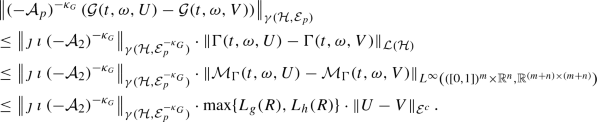
Hence, we obtain that \(\mathcal {G}:[0,T]\times \mathcal {E}^c\rightarrow \gamma (\mathcal {H},\mathcal {E}_p^{-\kappa _{G}})\) is locally Lipschitz continuous.
Using the assumptions (4.11) and (4.13) on the functions \(g_i\)’s and \(h_j\)’s and an analogous computation as above, we obtain that \(\mathcal {G}\) grows as required in Assumption (7) as a map \([0,T]\times \mathcal {E}^c\rightarrow \gamma (\mathcal {H},\mathcal {E}_p^{-\kappa _{G}})\).
 with
with  . Since
  chosen above. We apply a similar computation as in the proof of [
\(\square \)
In the following, we treat the special case when \(h_j\equiv 0\), \(j=1,\dots ,m\), that is, there is stochastic noise only in the vertices of the network. To rewrite equations (4.7) in the form (SCPn), we define the operator \(\mathcal {G}\) in a different way than it has been done in (4.18).
Instead of the operator in (4.17) we define \(\Gamma :[0,T]\times \Omega \times \mathcal {E}^c\rightarrow \mathcal {L}(\mathcal {E}_p)\) as
for \(U=\begin{pmatrix} u \\ r \end{pmatrix}\in \mathcal {E}^c\) and \(Y\in \mathcal {E}_p\) with
Because of the assumptions on the functions \(g_i\), \(\Gamma \) clearly maps into \(\mathcal {L}(\mathcal {E}_p).\)
Now, let
Then for all \(p\ge 2\), \(R\in \gamma (\mathcal {H},\mathcal {E}_p)\) with \(\mathcal {H}=\mathcal {E}_2\) holds since R has finite-dimensional range.
Now \(\mathcal {G}:[0,T]\times \Omega \times \mathcal {E}^c\rightarrow \gamma (\mathcal {H},\mathcal {E}_p)\) will be defined as
In this case we obtain a better regularity in Theorem 4.7.
Theorem 4.8
Let \(\mathcal {F}\), \(\widetilde{\mathcal {F}}\), \(\mathcal {G}\) and \(\mathcal {W}\) defined as in (4.14), (4.15), (4.24) and (4.21), respectively, and assume that \(h_j\equiv 0,\) \(j=1,\dots , m.\) Then for arbitrary \(q>2\) and for every \(\xi \in L^q(\Omega ,\mathscr {F}_0,\mathbb {P};\mathcal {E}^c)\) equation (SCPn) has a unique global mild solution in \(\mathcal {V}_{T,q}\).
Proof
We first chose \(p\ge 2\) such that
Hence, we can take \(\theta \) satisfying
We will apply Theorem 3.10 with \(\theta \) having this property and  . To this end we have to check Assumptions 3.7 again for the mappings in (SCPn), taking \(\mathcal {A}=\mathcal {A}_p\) for the p chosen above. This can be done in the same way as in the proof of Theorem 4.7 up to Assumption (7). The latter can be easily checked for
  for the operator \(\mathcal {G}:[0,T]\times \Omega \times \mathcal {E}^c\rightarrow \gamma (\mathcal {H},\mathcal {E}_p)\) defined in (4.24). If \(U,V\in \mathcal {E}^c\) with \(\Vert U\Vert _{\mathcal {E}^c},\Vert V\Vert _{\mathcal {E}^c}\le r,\) then
where \(L_{\mathcal {G}}^{(r)}\) is the maximum of the Lipschitz constants of the functions \(g_i\) on the ball \(\{x\in \mathbb {R}:|x|\le r\}\) (see (4.10)) and \(\Vert R\Vert _{\gamma (\mathcal {H},\mathcal {E}_p)}\) is finite.
Furthermore, applying (4.11), the last statement of Assumption (7) follows similarly as above; hence, there exists a constant \(c'>0\) such that
for all \((t,\omega ,U)\in [0,T]\times \Omega \times \mathcal {E}^c.\) \(\square \)
In the following theorem, we will state a result regarding the regularity of the mild solution of (SCPn) that exists according to Theorem 4.7. We will show that the trajectories of the solutions are actually continuous in the vertices of the graph; hence, they lie in the space
where (L, D(L)) is the boundary operator defined in (2.5). The space \(\mathcal {B}\) can be looked at as the Banach space of all continuous functions on the graph \(\mathsf {G}\) with norm
It is easy to see that
We can again prove the following continuous embeddings. In contrast to Corollary 4.3, also the first embedding will be dense.
Proposition 4.9
Let \(\mathcal {E}_p^{\theta }\) defined in (4.1) for \(p\in [1,\infty )\). Then for \(\theta > \frac{1}{2p}\) the following continuous, dense embeddings are satisfied:
Proof
According to Lemma 4.2(2), we have that for \(\theta > \frac{1}{2p}\)
holds. In [33, Lem. 3.6], we have proved that
where \(C_0[0,1]\) denotes such continuous functions that are 0 at the endpoints of the interval [0, 1]. Hence, combining this with (4.29) and using Sobolev imbedding, we obtain that for \(\theta >\frac{1}{2p}\) the continuous, dense embedding
is satisfied. Using (4.30) again, we have \(\mathcal {B}\hookrightarrow \mathcal {E}_p\), and the claim follows. \(\square \)
To the analogy of \(\mathcal {V}_{T,q}\), we define for a fixed \(T>0\) and \(q\ge 1\)
being a Banach space with norm
In the following, we will show that the trajectories of the solution of (SCPn) lie in \(\mathcal {B}\).
Theorem 4.10
Let \(\mathcal {F}\), \(\widetilde{\mathcal {F}}\), \(\mathcal {G}\) and \(\mathcal {W}\) defined as in (4.14), (4.15), (4.18) and (4.21), respectively. Let \(q>4\) be arbitrary. Then for every \(\xi \in L^{q}(\Omega ,\mathscr {F}_0,\mathbb {P};\mathcal {E}^c)\) equation (SCPn) has a unique global mild solution in \(\widetilde{\mathcal {V}}_{T,q}\).
Proof
By Theorem 4.7, there exists a global mild solution \(\mathcal {X}\in \mathcal {V}_{T,q}\), that is,
This solution satisfies the following implicit equation (see (3.5)):
where \(\mathcal {S}\) denotes the semigroup generated by \(\mathcal {A}_p\) on \(\mathcal {E}_p\) for some \(p\ge 2\) large enough, \(*\) denotes the usual convolution, \(\diamond \) denotes the stochastic convolution with respect to \(\mathcal {W}.\) We only have to show that for almost all \(\omega \in \Omega \) for the trajectories
holds. Then \(\mathcal {X}\in \widetilde{\mathcal {V}}_{T,q}\) is satisfied since the norms on \(\mathcal {E}^c\) and \(\mathcal {B}\) coincide and (4.31) is true. We will show (4.33) by showing it for all the three terms on the right-hand-side of (4.32).
We first fix \(0<\alpha <\frac{1}{2}\) and \(\eta > 0\) such that
holds. It is possible because of the assumption \(q>4\). Then, we choose  such that

is satisfied. We further fix \(p\ge 2\) such that
-
(1)
Using (4.28), we have that almost surely \(\xi \in \mathcal {E}^c\) holds. Hence, using the analiticity of \(\mathcal {S}\) on \(\mathcal {E}^c\) (see Proposition 4.4) and the obvious fact \(D(\mathcal {A})\subset \mathcal {B}\) (see (2.17)), we have that almost surely
$$\begin{aligned} \mathcal {S}(\cdot )\xi \in C((0,T];\mathcal {B})\cap L^{\infty }(0,T;\mathcal {B}) \end{aligned}$$(4.36)also holds.
-
(2)
For the deterministic convolution term with \(\mathcal {F}\) in (4.32), observe that by the choice of the constants
$$\begin{aligned} \frac{1}{2p}<\eta <1-\frac{1}{q} \end{aligned}$$(4.37)holds. We now apply [56, Lem. 3.6] with \(\alpha =1\), \(\theta =\lambda =0\), q instead of p and for \(\eta \). Hence, we obtain that there exist constants \(C\ge 0\) and \(\varepsilon >0\) such that
$$\begin{aligned} \Vert \mathcal {S}*\mathcal {F}(\cdot ,\mathcal {X}(\cdot ))(t)\Vert _{C([0,T];\mathcal {E}_p^{\eta })}\le CT^{\varepsilon }\Vert \mathcal {F}(\cdot ,\mathcal {X}(\cdot ))\Vert _{L^q(0,T;\mathcal {E}_p)}. \end{aligned}$$(4.38)Taking the qth power on the right-hand-side of (4.38), using Corollary 4.3 and (4.23), we conclude that
$$\begin{aligned} \Vert \mathcal {F}(\cdot ,\mathcal {X}(\cdot ))\Vert ^q_{L^q(0,T;\mathcal {E}_p)}&=\int _0^T\Vert \mathcal {F}(s,\mathcal {X}(s))\Vert ^q_{\mathcal {E}_p}\, \mathrm{d}s\\&\lesssim \int _0^T\Vert \mathcal {F}(s,\mathcal {X}(s))\Vert ^q_{\mathcal {E}^c}\, \mathrm{d}s\\&\lesssim \int _0^T(1+\Vert \mathcal {X}(s)\Vert ^{K\cdot q}_{\mathcal {E}^c})\, \mathrm{d}s\\&\lesssim (1+\sup _{t\in [0,T]}\Vert \mathcal {X}(t)\Vert ^{K\cdot q}_{\mathcal {E}^c}). \end{aligned}$$Hence,
$$\begin{aligned} \Vert \mathcal {S}*\mathcal {F}(\cdot ,\mathcal {X}(\cdot ))\Vert ^q_{C([0,T];\mathcal {E}_p^{\eta })} \le C_T\cdot \left( 1+\sup _{t\in [0,T]}\Vert \mathcal {X}(t)\Vert _{\mathcal {E}^c}^{K\cdot q}\right) . \end{aligned}$$By Proposition 4.9 and (4.37), we obtain that \(\mathcal {S}*\mathcal {F}(\cdot ,\mathcal {X}(\cdot )) \in C([0,T];\mathcal {B})\) holds and for a positive constant \(C_T'>0\)
$$\begin{aligned} \Vert \mathcal {S}*\mathcal {F}(\cdot ,\mathcal {X}(\cdot ))\Vert ^q_{C([0,T];\mathcal {B})} \le C_T'\cdot \left( 1+\sup _{t\in [0,T]}\Vert \mathcal {X}(t)\Vert _{\mathcal {E}^c}^{K\cdot q}\right) . \end{aligned}$$(4.39)Since we know by (4.31) that for almost all \(\omega \in \Omega \) the right-hand-side is finite, we obtain that the left-hand side is almost surely finite.
-
(3)
For the deterministic convolution term with \(\widetilde{\mathcal {F}}\) in (4.32) we proceed similarly as before. We apply [56, Lem. 3.6] with \(\alpha =1\), \(\lambda =0\), \(\theta =\frac{1}{2}\), q instead of p and for \(\eta \). We obtain that there exist constants \(C\ge 0\) and \(\varepsilon >0\) such that
$$\begin{aligned} \Vert \mathcal {S}*\widetilde{\mathcal {F}}(\mathcal {X}(\cdot ))(t)\Vert _{C([0,T];\mathcal {E}_p^{\eta })}\le CT^{\varepsilon }\Vert \widetilde{\mathcal {F}}(\mathcal {X}(\cdot ))\Vert _{L^q(0,T;\mathcal {E}_p^{-\frac{1}{2}})}. \end{aligned}$$(4.40)Taking the qth power on the right-hand-side of (4.40) and using (4.20) we conclude that
$$\begin{aligned}&\Vert \widetilde{\mathcal {F}}(\mathcal {X}(\cdot ))\Vert ^q_{L^q(0,T;\mathcal {E}_p^{-\frac{1}{2}})}=\int _0^T\Vert \widetilde{\mathcal {F}}(\mathcal {X}(s))\Vert ^q_{\mathcal {E}_p^{-\frac{1}{2}}}\, \mathrm{d}s\\&\quad \lesssim \int _0^T\Vert \mathcal {X}(s)\Vert ^{q}_{\mathcal {E}^c}\, \mathrm{d}s\lesssim \sup _{t\in [0,T]}\Vert \mathcal {X}(t)\Vert ^{q}_{\mathcal {E}^c}. \end{aligned}$$Hence,
$$\begin{aligned} \Vert \mathcal {S}*\widetilde{\mathcal {F}}(\mathcal {X}(\cdot ))\Vert ^q_{C([0,T];\mathcal {E}_p^{\eta })} \le C_T\cdot \sup _{t\in [0,T]}\Vert \mathcal {X}(t)\Vert _{\mathcal {E}^c}^{q}. \end{aligned}$$By Proposition 4.9 and (4.37), we obtain that \(\mathcal {S}*\widetilde{\mathcal {F}}(\mathcal {X}(\cdot )) \in C([0,T];\mathcal {B})\) holds and for a positive constant \(C_T'>0\)
$$\begin{aligned} \Vert \mathcal {S}*\widetilde{\mathcal {F}}(\mathcal {X}(\cdot ))\Vert ^q_{C([0,T];\mathcal {B})} \le C_T'\cdot \sup _{t\in [0,T]}\Vert \mathcal {X}(t)\Vert _{\mathcal {E}^c}^{q}. \end{aligned}$$Since we know by (4.31) that for almost all \(\omega \in \Omega \) the right-hand side is finite, we obtain that the left-hand side is almost surely finite.
-
(4)
We now prove that for the stochastic convolution term \(\mathcal {S}\diamond \mathcal {G}(\cdot ,\mathcal {X}(\cdot )){\in } C([0,T];\mathcal {B})\) almost surely holds by showing that
$$\begin{aligned} \mathbb {E}\left\| \mathcal {S}\diamond \mathcal {G}(\cdot ,\mathcal {X}(\cdot ))\right\| ^q_{C([0,T];\mathcal {B})} \end{aligned}$$is finite. By (4.34), we can apply [56, Prop. 4.2] with \(\lambda =0\),
 , q instead of p, \(\alpha \) and \(\eta \), obtaining that there exist \(\varepsilon >0\) and \(C\ge 0\) such that
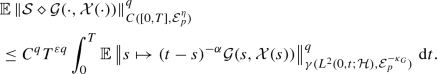
In the following, we proceed similarly as done in the proof of [35, Thm. 4.3], with \(N=1\) and q instead of p. Since
 is a Banach space of type 2 (because \(\mathcal {E}_p\) is of that type), the continuous embedding
  (4.41)
holds. Using this, Young’s inequality and the growth property of \(\mathcal {G}\) (see the proof of Theorem 4.7), respectively, we obtain the following estimates
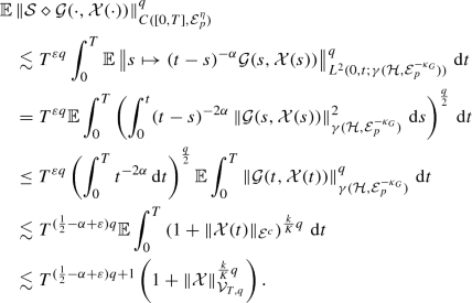
Hence, for each \(T>0\) there exists a constant \(C_{T}>0\) such that
$$\begin{aligned} \mathbb {E}\left\| \mathcal {S}\diamond \mathcal {G}(\cdot ,\mathcal {X}(\cdot ))\right\| ^q_{C([0,T],\mathcal {E}_p^{\eta })} \le C'_{T}\cdot \left( 1+\Vert \mathcal {X}\Vert ^{\frac{k}{K}q}_{\mathcal {V}_{T,q}}\right) . \end{aligned}$$Using that \(\frac{k}{K}<1\), it follows that
$$\begin{aligned} \mathbb {E}\left\| \mathcal {S}\diamond \mathcal {G}(\cdot ,\mathcal {X}(\cdot ))\right\| ^q_{C([0,T];\mathcal {E}_p^{\eta })} \le C''_{T}\cdot \left( 1+\Vert \mathcal {X}\Vert ^{q}_{\mathcal {V}_{T,q}}\right) . \end{aligned}$$By Proposition 4.9 and (4.35) we obtain that for a positive constant \(\tilde{C}_T>0\)
$$\begin{aligned} \mathbb {E}\left\| \mathcal {S}\diamond \mathcal {G}(\cdot ,\mathcal {X}(\cdot ))\right\| ^q_{C([0,T];\mathcal {B})} \le \tilde{C}_T\cdot \left( 1+\Vert \mathcal {X}\Vert ^{q}_{\mathcal {V}_{T,q}}\right) \end{aligned}$$(4.42)is satisfied.
 , q instead of p,
 is a Banach space of type 2 (because

Finally, by (4.36), (4.39) and (4.42), we obtain (4.33), and hence, the proof is complete. \(\square \)
We again treat the case when \(h_j\equiv 0\), \(j=1,\dots ,m\) separately by defining the operator \(\mathcal {G}\) as in (4.24) to obtain better regularity for the solutions.
Theorem 4.11
Let \(\mathcal {F}\), \(\widetilde{\mathcal {F}}\), \(\mathcal {G}\) and \(\mathcal {W}\) defined as in (4.14), (4.15), (4.24) and (4.21), respectively, and assume that \(h_j\equiv 0,\) \(j=1,\dots m.\) Then for arbitrary \(q>2\) and for every \(\xi \in L^{q}(\Omega ,\mathscr {F}_0,\mathbb {P};\mathcal {E}^c)\) equation (SCPn) has a unique global mild solution in \(\widetilde{\mathcal {V}}_{T,q}\).
Proof
The claim can be proved analogously to Theorem 4.10 except for step (4). To show that in this case \(\mathcal {S}\diamond \mathcal {G}(\cdot ,\mathcal {X}(\cdot ))\in C([0,T];\mathcal {B})\) almost surely holds we first fix \(0<\alpha <\frac{1}{2}\) and \(p\ge 2\) such that
holds (it is possible since \(q>2\)). We further choose \(\eta >0\) such that
is satisfied. Applying [56, Prop. 4.2] with \(\theta =\lambda =0\) and q instead of p, we have that there exist \(\varepsilon >0\) and \(C\ge 0\) such that
In the following we proceed similarly as done in the proof of [35, Thm. 4.3], with \(N=1\) and q instead of p. Since \(\mathcal {E}_p\) is a Banach space of type 2, we can use the continuous embedding
Young’s inequality and (4.26), respectively, to obtain the following estimates
Using that \(\frac{k}{K}<1\), we conlcude that there exists a constant \(C''_{T}\) such that
holds. By Proposition 4.9 and (4.44) we obtain that for a positive constant \(\tilde{C}_T>0\)
is satisfied and thus
almost surely. \(\square \)
Remark 4.12
If, in Theorems 4.10 and 4.11, the initial condition satisfies \(\xi \in L^{q}(\Omega ,\mathscr {F}_0,\mathbb {P};\mathcal {B})\), then the global mild solution belongs even to \(L^q(\Omega ;C([0,T];\mathcal {B}))\) instead of \(\widetilde{\mathcal {V}}_{T,q}\). This follows from the fact that the semigroup \(\mathcal {S}\) is strongly continuous on \(\mathcal {B}\) which can be shown by a completely analogous argument as in [34, Prop. 3.8].
References
Wolfgang Arendt, Charles J. K. Batty, Matthias Hieber, and Frank Neubrander. Vector-valued Laplace transforms and Cauchy problems, volume 96 of Monographs in Mathematics. Birkhäuser/Springer Basel AG, Basel, second edition, 2011.
Fernando Albiac and Nigel J. Kalton. Topics in Banach space theory, volume 233 of Graduate Texts in Mathematics. Springer, [Cham], second edition, 2016. With a foreword by Gilles Godefory.
F. Ali Mehmeti. Problèmes de transmission pour des équations des ondes linéaires et quasilinéaires. In Hyperbolic and holomorphic partial differential equations, Travaux en Cours, pages 75–96. Hermann, Paris, 1984.
Felix Ali Mehmeti. A characterization of a generalized \(C^\infty \)-notion on nets. Integral Equations Operator Theory, 9(6):753–766, 1986.
Felix Ali Mehmeti. Nonlinear waves in networks, volume 80 of Mathematical Research. Akademie-Verlag, Berlin, 1994.
Felix Ali Mehmeti, Joachim von Below, and Serge Nicaise, editors. Partial differential equations on multistructures, volume 219 of Lecture Notes in Pure and Applied Mathematics. Marcel Dekker, Inc., New York, 2001.
Wolfgang Arendt. Semigroups and evolution equations: functional calculus, regularity and kernel estimates. In Evolutionary equations. Vol. I, Handb. Differ. Equ., pages 1–85. North-Holland, Amsterdam, 2004.
W. Arendt and A. F. M. ter Elst. Gaussian estimates for second order elliptic operators with boundary conditions. J. Operator Theory, 38(1):87–130, 1997.
Zdzisł aw Brzeźniak and Dariusz Ga̧tarek. Martingale solutions and invariant measures for stochastic evolution equations in Banach spaces. Stochastic Process. Appl., 84(2):187–225, 1999.
Stefano Bonaccorsi and Delio Mugnolo. Existence of strong solutions for neuronal network dynamics driven by fractional Brownian motions. Stoch. Dyn., 10(3):441–464, 2010.
Stefano Bonaccorsi, Carlo Marinelli, and Giacomo Ziglio. Stochastic FitzHugh-Nagumo equations on networks with impulsive noise. Electron. J. Probab., 13:no. 49, 1362–1379, 2008.
Zdzisł aw Brzeźniak and Szymon Peszat. Space-time continuous solutions to SPDE’s driven by a homogeneous Wiener process. Studia Math., 137(3):261–299, 1999.
Donald L. Burkholder. Martingales and singular integrals in Banach spaces. In Handbook of the geometry of Banach spaces, Vol. I, pages 233–269. North-Holland, Amsterdam, 2001.
Stefano Bonaccorsi and Giacomo Ziglio. Existence and stability of square-mean almost periodic solutions to a spatially extended neural network with impulsive noise. Random Oper. Stoch. Equ., 22(1):17–29, 2014.
Carla Cattaneo. The spectrum of the continuous Laplacian on a graph. Monatsh. Math., 124(3):215–235, 1997.
Francesco Cordoni and Luca Di Persio. Gaussian estimates on networks with dynamic stochastic boundary conditions. Infin. Dimens. Anal. Quantum Probab. Relat. Top., 20(1):1750001, 23, 2017.
Francesco Cordoni and Luca Di Persio. Stochastic reaction–diffusion equations on networks with dynamic time-delayed boundary conditions. J. Math. Anal. Appl., 451(1):583–603, 2017.
Sandra Cerrai. Second order PDE’s in finite and infinite dimension, volume 1762 of Lecture Notes in Mathematics. Springer-Verlag, Berlin, 2001. A probabilistic approach.
Sandra Cerrai. Stochastic reaction-diffusion systems with multiplicative noise and non-Lipschitz reaction term. Probab. Theory Related Fields, 125(2):271–304, 2003.
Carla Cattaneo and Luigi Fontana. D’Alembert formula on finite one-dimensional networks. J. Math. Anal. Appl., 284(2):403–424, 2003.
Sandra Cerrai and Mark Freidlin. SPDEs on narrow domains and on graphs: an asymptotic approach. Ann. Inst. Henri Poincaré Probab. Stat., 53(2):865–899, 2017.
E. B. Davies. Heat kernels and spectral theory, volume 92 of Cambridge Tracts in Mathematics. Cambridge University Press, Cambridge, 1990.
Giuseppe Da Prato and Jerzy Zabczyk. Nonexplosion, boundedness, and ergodicity for stochastic semilinear equations. J. Differential Equations, 98(1):181–195, 1992.
Luca Di Persio and Giacomo Ziglio. Gaussian estimates on networks with applications to optimal control. Netw. Heterog. Media, 6(2):279–296, 2011.
Xuan Thinh Duong. \(H_\infty \) functional calculus of second order elliptic partial differential operators on \(L^p\) spaces. In Miniconference on Operators in Analysis (Sydney, 1989), volume 24 of Proc. Centre Math. Anal. Austral. Nat. Univ., pages 91–102. Austral. Nat. Univ., Canberra, 1990.
Klaus-Jochen Engel and Marjeta Kramar Fijavž. Waves and diffusion on metric graphs with general vertex conditions. Evol. Equ. Control Theory, 8(3):633–661, 2019.
Klaus-Jochen Engel and Rainer Nagel. One-parameter semigroups for linear evolution equations, volume 194 of Graduate Texts in Mathematics. Springer-Verlag, New York, 2000. With contributions by S. Brendle, M. Campiti, T. Hahn, G. Metafune, G. Nickel, D. Pallara, C. Perazzoli, A. Rhandi, S. Romanelli and R. Schnaubelt.
Markus Haase. The functional calculus for sectorial operators, volume 169 of Operator Theory: Advances and Applications. Birkhäuser Verlag, Basel, 2006.
Edwin Hewitt and Karl Stromberg. Real and abstract analysis. Springer-Verlag, New York-Heidelberg, 1975. A modern treatment of the theory of functions of a real variable, Third printing, Graduate Texts in Mathematics, No. 25.
Mark Kac. Can one hear the shape of a drum? Amer. Math. Monthly, 73(4, part II):1–23, 1966.
Marjeta Kramar Fijavž, Delio Mugnolo, and Eszter Sikolya. Variational and semigroup methods for waves and diffusion in networks. Appl. Math. Optim., 55(2):219–240, 2007.
Marjeta Kramar and Eszter Sikolya. Spectral properties and asymptotic periodicity of flows in networks. Math. Z., 249(1):139–162, 2005.
Mihály Kovács and Eszter Sikolya. On the stochastic Allen-Cahn equation on networks with multiplicative noise. Electron. J. Qual. Theory Differ. Equ., pages Paper No. 7, 1–24, 2021.
Mihály Kovács and Eszter Sikolya. On the stochastic Allen-Cahn equation on networks with multiplicative noise. https://arxiv.org/abs/2011.11359v2, 2021.
Markus Kunze and Jan van Neerven. Continuous dependence on the coefficients and global existence for stochastic reaction diffusion equations. J. Differential Equations, 253(3):1036–1068, 2012.
Markus Kunze and Jan van Neerven. Continuous dependence on the coefficients and global existence for stochastic reaction diffusion equations. https://arxiv.org/abs/1104.4258, 2019.
J. E. Lagnese, Günter Leugering, and E. J. P. G. Schmidt. Modeling, analysis and control of dynamic elastic multi-link structures. Systems & Control: Foundations & Applications. Birkhäuser Boston, Inc., Boston, MA, 1994.
Gunter Lumer. Espaces ramifiés, et diffusions sur les réseaux topologiques. C. R. Acad. Sci. Paris Sér. A-B, 291(12):A627–A630, 1980.
Alessandra Lunardi. Analytic semigroups and optimal regularity in parabolic problems, volume 16 of Progress in Nonlinear Differential Equations and their Applications. Birkhäuser Verlag, Basel, 1995.
Celso Martínez Carracedo and Miguel Sanz Alix. The theory of fractional powers of operators, volume 187 of North-Holland Mathematics Studies. North-Holland Publishing Co., Amsterdam, 2001.
Gustavo A. Muñoz, Yannis Sarantopoulos, and Andrew Tonge. Complexifications of real Banach spaces, polynomials and multilinear maps. Studia Math., 134(1):1–33, 1999.
Delio Mugnolo and Silvia Romanelli. Dynamic and generalized Wentzell node conditions for network equations. Math. Methods Appl. Sci., 30(6):681–706, 2007.
Tamás Mátrai and Eszter Sikolya. Asymptotic behavior of flows in networks. Forum Math., 19(3):429–461, 2007.
Delio Mugnolo. Gaussian estimates for a heat equation on a network. Netw. Heterog. Media, 2(1):55–79, 2007.
Delio Mugnolo. Asymptotics of semigroups generated by operator matrices. Arab. J. Math. (Springer), 3(4):419–435, 2014.
Delio Mugnolo. Semigroup methods for evolution equations on networks. Understanding Complex Systems. Springer, Cham, 2014.
S. Nicaise. Some results on spectral theory over networks, applied to nerve impulse transmission. In Orthogonal polynomials and applications (Bar-le-Duc, 1984), volume 1171 of Lecture Notes in Math., pages 532–541. Springer, Berlin, 1985.
El Maati Ouhabaz. Analysis of heat equations on domains, volume 31 of London Mathematical Society Monographs Series. Princeton University Press, Princeton, NJ, 2005.
Szymon Peszat. Existence and uniqueness of the solution for stochastic equations on Banach spaces. Stochastics Stochastics Rep., 55(3-4):167–193, 1995.
Hans Triebel. Interpolation theory, function spaces, differential operators, volume 18 of North-Holland Mathematical Library. North-Holland Publishing Co., Amsterdam-New York, 1978.
Joachim von Below. A characteristic equation associated to an eigenvalue problem on \(c^2\)-networks. Linear Algebra Appl., 71:309–325, 1985.
Joachim von Below. Classical solvability of linear parabolic equations on networks. J. Differential Equations, 72(2):316–337, 1988.
Joachim von Below. Sturm-Liouville eigenvalue problems on networks. Math. Methods Appl. Sci., 10(4):383–395, 1988.
Joachim von Below and Serge Nicaise. Dynamical interface transition in ramified media with diffusion. Comm. Partial Differential Equations, 21(1-2):255–279, 1996.
Jan van Neerven. The adjoint of a semigroup of linear operators, volume 1529 of Lecture Notes in Mathematics. Springer-Verlag, Berlin, 1992.
J. M. A. M. van Neerven, M. C. Veraar, and L. Weis. Stochastic evolution equations in UMD Banach spaces. J. Funct. Anal., 255(4):940–993, 2008.
Acknowledgements
We thank the referee for the constructive criticism and suggestions which helped to improve the quality of the manuscript significantly.
Funding
Open access funding provided by Eötvös Loránd University.
Author information
Authors and Affiliations
Corresponding author
Additional information
Publisher's Note
Springer Nature remains neutral with regard to jurisdictional claims in published maps and institutional affiliations.
M. Kovács was supported by Marsden Fund of the Royal Society of New Zealand Grant No. 18-UOO-143, VR Grant Number 2017-04274 and NKFI Grant Number K-131501.
Appendices
Proof of Proposition 2.3
We defined the form  in (2.13)–(2.14) as

on the Hilbert space \(\mathcal {E}_2\) with dense domain

The operator associated with a form is defined in Definition 2.2 as

The operator \(\left( \mathcal {A}_2,D(\mathcal {A}_2)\right) \) from (2.10)–(2.11) is defined on \(\mathcal {E}_2\) as
with domain
Proposition A.1
The operator associated with the form  is \(\left( \mathcal {A}_2,D(\mathcal {A}_2)\right) \).
Proof
Denote by \(\left( \mathcal {B},D(\mathcal {B})\right) \) the operator associated with  . Let us first show that \(\mathcal {A}_2\subset \mathcal {B}\). Take \(U=\left( {\begin{matrix}u\\ r\end{matrix}}\right) \in D(\mathcal {A}_2)\). Then for all \(H=\Big ({\begin{matrix}h\\ d\end{matrix}}\Big )\in \mathcal {V}\)

Using the entries (2.1) of the incidence matrix \(\Phi \), the first term above can be written as
Observe now that by the definition of \(\mathcal {V}\),
holds. Changing the sums, and using (2.3) and (2.8), we have that
The second term in (A.1) is by definition (2.6)–(2.7) of \((A_{max},D(A_{max}))\)
which makes sense because \(A_{max}u\in E_2\). Hence,

The proof of the inclusion \(\mathcal {A}_2\subset \mathcal {B}\) is thus completed.
To check the converse inclusion \(\mathcal {B}\subset \mathcal {A}_2\) take \(U=\left( {\begin{matrix}u\\ r\end{matrix}}\right) \in D(\mathcal {B})\). By definition, there exists \(V=\Big ({\begin{matrix}v\\ q\end{matrix}}\Big )\in \mathcal {E}_2\) such that

and \(\mathcal {B}U=-V\). In particular,
for all \(H=\Big ({\begin{matrix}h\\ d\end{matrix}}\Big )\in \mathcal {V}\), hence also for all \(h^j\) of the form
and \(L h^j=d=0_{\mathbb {C}^n}.\) From this follows that (A.2) in fact implies
By definition of weak derivative this means that \(c_j\cdot u_j'\in H^1(0,1)\) for all \(j=1,\ldots ,m\). Since \(0<c_j\in H^1(0,1)\), it follows that in fact \(u_j'\in H^1(0,1)\) for all \(j=1,\ldots ,m\). We conclude that \(u\in \left( H^2(0,1)\right) ^m\); hence, by \(U\in \mathcal {V}\), also \(U\in D(\mathcal {A}_2)\) holds.
Moreover, integrating by parts as in (A.1) we see—analogously to the first part of the proof—that if (A.2) holds for some \(H=\Big ({\begin{matrix}h\\ d\end{matrix}}\Big )\in \mathcal {V}\), then
That is,

for arbitrary \(H\in \mathcal {V}\); hence, \( \mathcal {A}_2 U=-V=\mathcal {B}U\) and this completes the proof. \(\square \)
Proof of Proposition 2.4
We defined the spaces \(\mathcal {E}_p\) for \(p\in [1,\infty ]\) in (2.15). In the subsequent lemma we prove crucial properties of the semigroup \((\mathcal {T}_2(t))_{t\ge 0}\) that will imply its extendability to the spaces \(\mathcal {E}_p\). The proof is similar to that of [42, Lem. 4.1 and Prop. 5.3] except the fact that we have non-diagonal matrix M. Therefore, we give it in details.
Lemma B.1
If Assumption 2.1 holds for M, then the semigroup \((\mathcal {T}_2(t))_{t\ge 0}\) on \(\mathcal {E}_2\), generated by \(\mathcal {A}_2\), is sub-Markovian, i.e., it is real, positive, and contractive on \(\mathcal {E}_\infty \).
Proof
By [48, Prop. 2.5, Thm. 2.7, and Cor. 2.17], we need to check that the following criteria are verified for the domain \(\mathcal {V}\) of  , see (2.14):
-
 ,
, -
 ,
, -
 .
.
 ,
, ,
, .
.It is clear that \(\overline{k}\in H^1(0,1)\) if \(k\in H^1(0,1)\). Further, if k is real valued, then \(\vert k\vert \in H^1(0,1)\) and \(\vert k\vert '={{\,\mathrm{sgn}\,}}k\cdot k'\), and if \(0\le k\), then \(1\wedge k\in H^1(0,1)\) with \((1\wedge k)'=k'\cdot {\mathbf {1}}_{\{k<1\}}\) and \(((k-1)^{+})'=k'\cdot {\mathbf {1}}_{\{k>1\}}\).
Take any
By definition we have \(\overline{u_j}=(\overline{u})_j\), \(1\le j\le m\). It follows from the above arguments that \(\overline{f}\in \left( H^1(0,1)\right) ^m\), and one can see that
Hence, \(\overline{U}\in \mathcal {V}\). Moreover, the first two sums of  are sums of m integrals. Recall that all the weights are real-valued, nonnegative functions. Since all the integrated functions are real-valued, and the third sum is the sum of real numbers, it follows that
  . Thus, the first criterion has been checked.
Moreover, if U is a real-valued, then \(\vert u_j\vert =\vert u\vert _j\), \(1\le j\le m\), \(\vert r_i\vert =\vert r\vert _i\), \(1\le i\le n\), and one sees as above that \(\vert U\vert \in \mathcal {V}\). In particular, \(\vert \vert u\vert '\vert ^2=\vert u'\vert ^2\), and

Let us investigate the third term. For r real
and
For \(i\ne k\), by Assumption 2.1.(2) we have
Since
trivially holds, we obtain that \(\langle M\vert r\vert ,\vert r \vert \rangle \ge \langle Mr,r\rangle \) for all r real, and by (B.1),

Finally, take \(0\le U=\left( {\begin{matrix} u\\ r\end{matrix}}\right) \in \mathcal {V}\). Then
with all the functions \(1\wedge u_j\in H^1(0,1)\), hence \(1\wedge u\in \left( H^1(0,1)\right) ^m\). Clearly,
i.e., \(1\wedge U\in \mathcal {V}\). Furthermore,

Using Assumption 2.1 and [46, Ex. 4.44(3)], we conclude that M generates a sub-Markovian semigroup; hence, by [48, Cor. 2.17], for \(r\ge 0\)
holds. We have checked also the third criterion; thus, the claim follows. \(\square \)
Rights and permissions
Open Access This article is licensed under a Creative Commons Attribution 4.0 International License, which permits use, sharing, adaptation, distribution and reproduction in any medium or format, as long as you give appropriate credit to the original author(s) and the source, provide a link to the Creative Commons licence, and indicate if changes were made. The images or other third party material in this article are included in the article’s Creative Commons licence, unless indicated otherwise in a credit line to the material. If material is not included in the article’s Creative Commons licence and your intended use is not permitted by statutory regulation or exceeds the permitted use, you will need to obtain permission directly from the copyright holder. To view a copy of this licence, visit http://creativecommons.org/licenses/by/4.0/.
About this article

Cite this article
Kovács, M., Sikolya, E. Stochastic reaction–diffusion equations on networks. J. Evol. Equ. 21, 4213–4260 (2021). https://doi.org/10.1007/s00028-021-00719-w
Accepted:
Published:
Issue Date:
DOI: https://doi.org/10.1007/s00028-021-00719-w