
Uncertainty Estimation in Hydrogeological Forecasting with Neural Networks: Impact of Spatial Distribution of Rainfalls and Random Initialization of the Model

 , ,
, ,
Abstract
:1. Introduction
2. Material and Methods
2.1. Neural Network Models
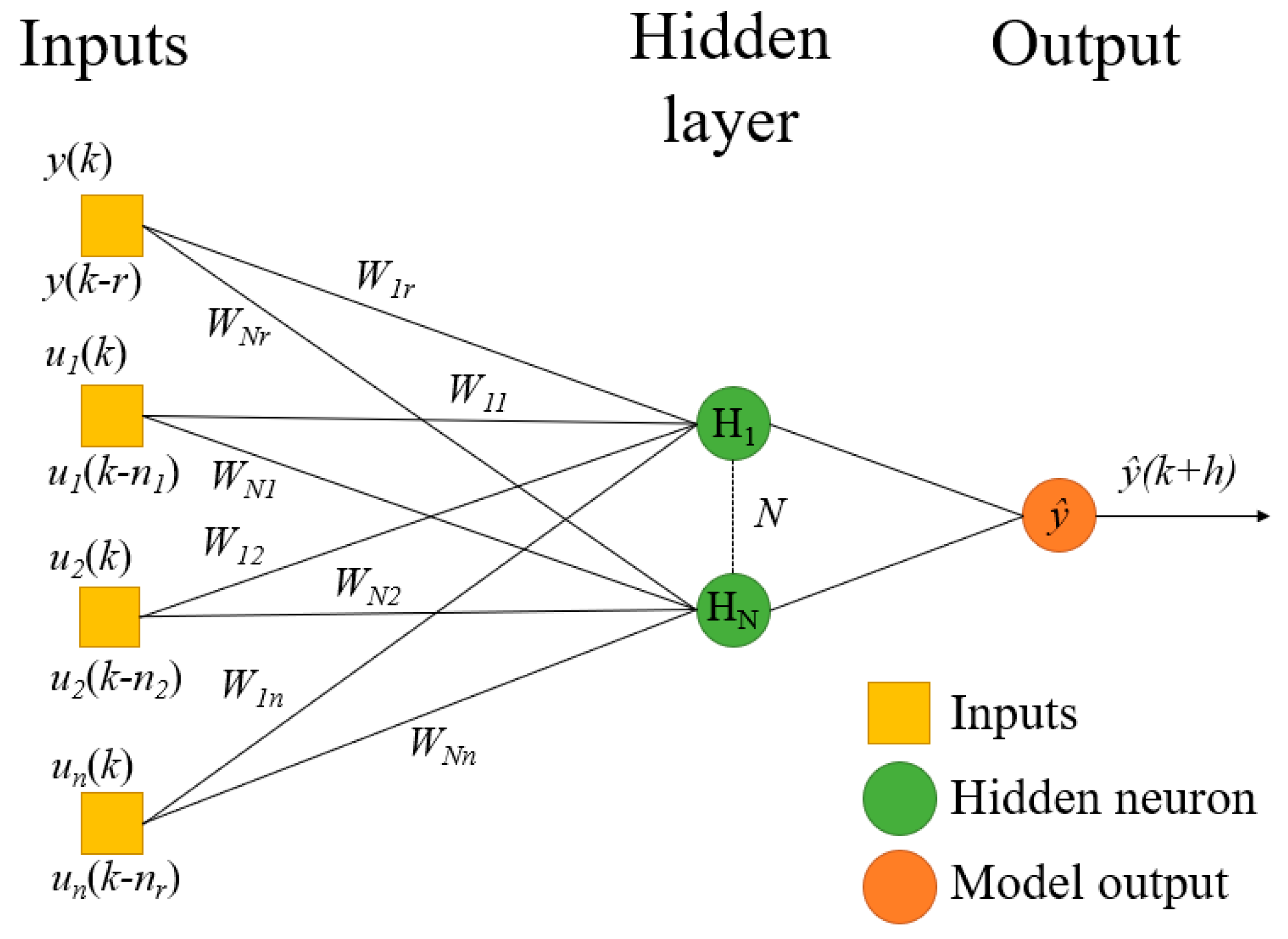
2.1.1. Definitions
2.1.2. Role of Time in Neural Networks Models
2.1.3. Training and Overfitting
2.1.4. Regularization Methods
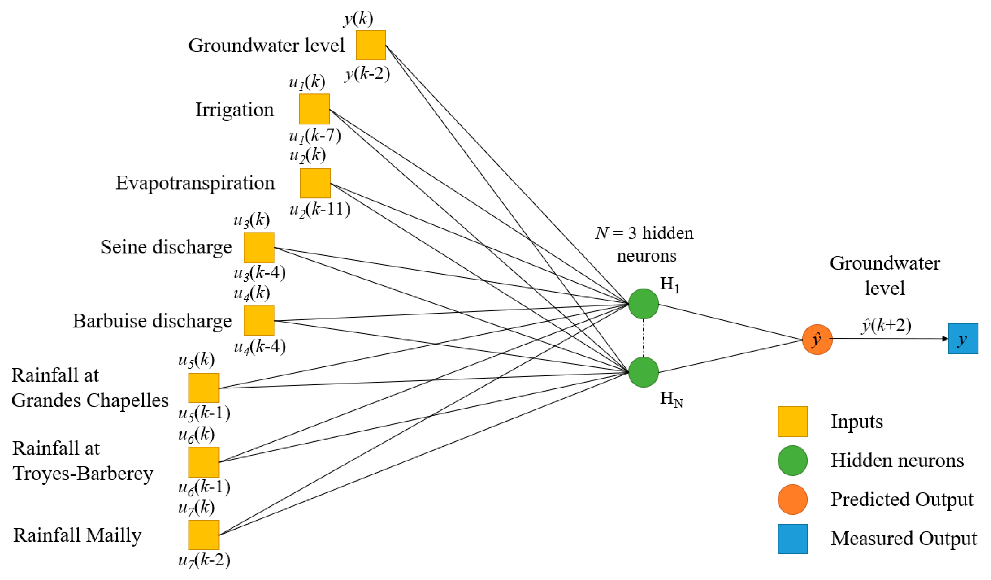
2.1.5. Model Design
- -
- The window widths of the different (exogenous) input variables (nr in Equations (1)–(3)).
- -
- The “order” of the model, corresponding to the window width of the estimated (or observed, if the model is a feed-forward) targeted variable (output variable), for previous time-steps, applied at the input of the model (r in Equations (2) and (3)).
- -
- The number of neurons in the hidden layers: N.
2.2. Study Area: The Champagne Chalk Groundwater Basin
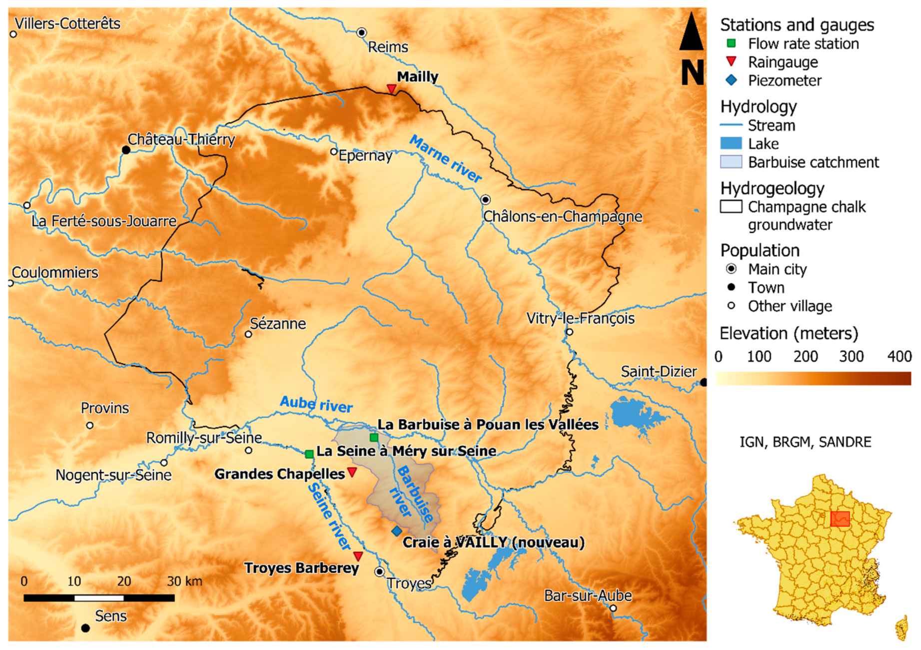
2.2.1. Field Study Presentation
- LocationLocated in Northern France, in the Grand-Est region, the Champagne chalk groundwater basin area is estimated at 5927 sq.km. It corresponds mainly to the drainage of the rivers Marne and Aube, delimited by piezometric ridges characterized as follows: chalk limit on the eastern part, tertiary rocks on the western part, other hydrogeological basins on the northern limit, the Seine river for the southern part and, as a bedrock, marlstones [23]. Elevation varies from 40 to 286 m.a.s.l. (Figure 2).
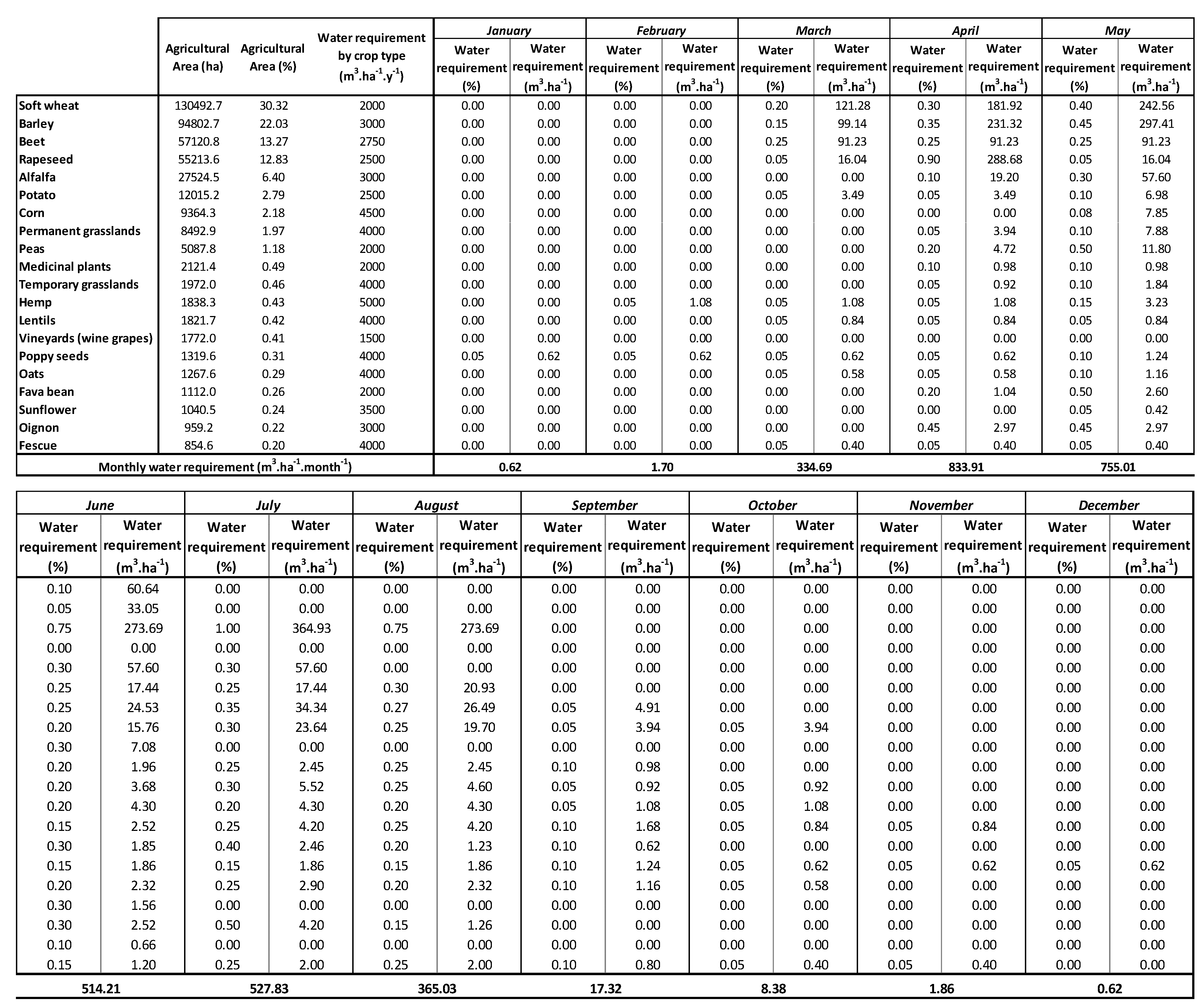
- Water useWater is mainly used for tap water production and agriculture [23]. Annual water withdrawals via studied piezometer made on average between 2012 and 2017 are 17,393 m3, however, showing a decreasing trend [24]. Water is also used for agriculture, with 61.5% of groundwater withdrawal for irrigation in 2017 (against 38.5% for tap water production) in Vailly (location of the studied piezometer) and neighboring towns [25].
- Climate
- Geology and groundwater behaviorThis basin is mainly composed of chalk, and limestones to a lesser proportion, with sands and clay along the hydrographic network [27,28]. Intense shallow fracturing, mainly caused by climate action, has developed a significant permeability especially near the hydrographic network. Groundwater recharge time in the champagne basin is estimated at 100 days in our study piezometer (Craie à Vailly (nouveau)) [29], and the underground levels can increase from 6 m to 25 m [23,30]. Groundwater levels, especially in the Barbuise catchment area, which is close to the study piezometer, are influenced by the shallow water [27]. Consequently, the Barbuise river discharge is strongly correlated to piezometric levels at Craie à Vailly [27,29].
2.2.2. Database Presentation
- Troyes-Barberey (RTB) (precipitation and potential evapotranspiration),
- Grandes-Chapelles (RGC) (precipitation),
- Mailly (RMA) (precipitation)
2.3. Quality Criteria
2.3.1. Quality of Fitting and Prediction
- The persistency criterion
2.3.2. Uncertainties Quantification
- Prediction Interval Coverage Probability
- Mean Prediction Interval
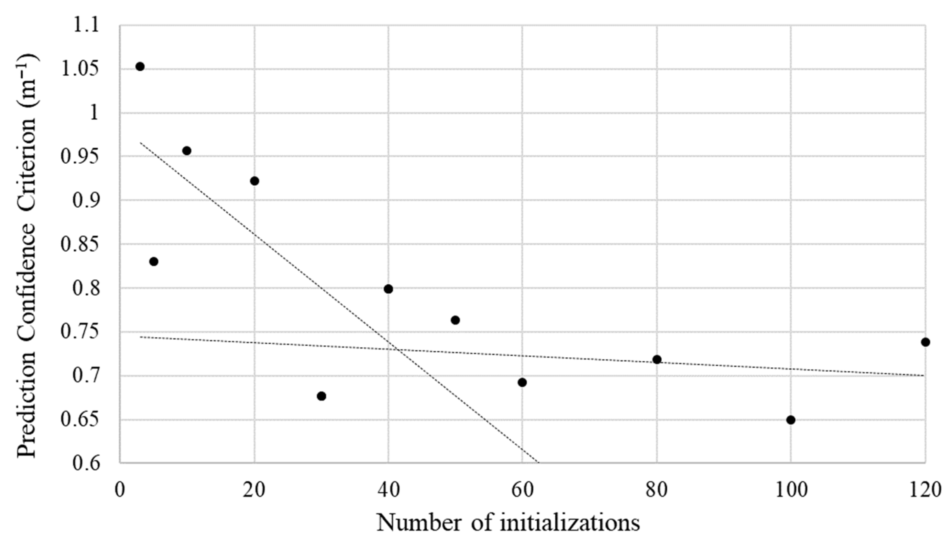
- Prediction Confidence Criterion
2.4. Uncertainties Linked to the Initialization of the Parameters and to the Spatial Variability of the Rains
2.4.1. Variability Due to the Initialization of Parameters
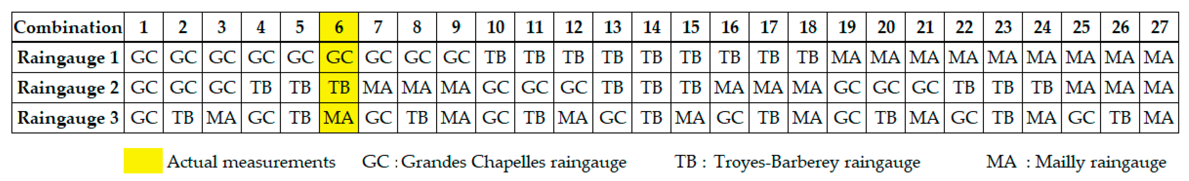
2.4.2. Spatial Rainfall Variability
2.5. Estimation of Empirical Confidence Intervals Using Probability Density Functions
2.5.1. Method
- -
- Establishing the frequencies of appearance of the water level classes histogram; this is then considered as an empirical probability density function (pdf) of the data;
- -
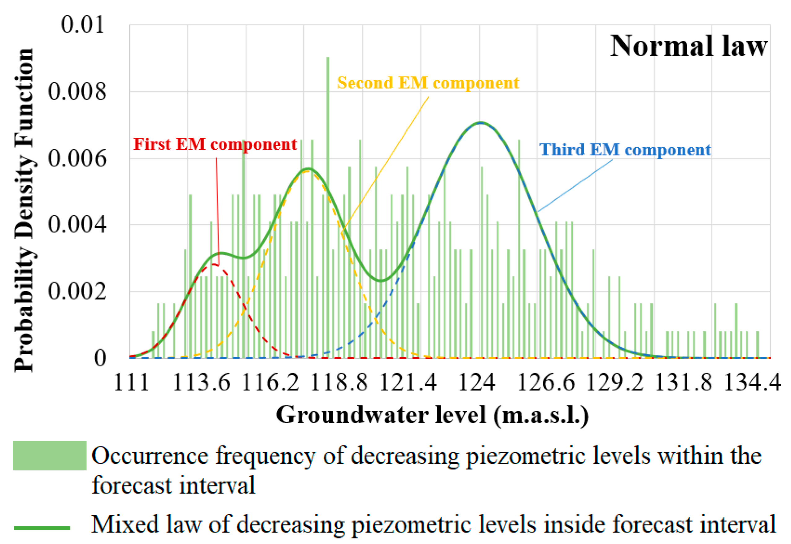
- Fitting a theoretical well-known pdf, for example the normal one, to the empirical pdf by adjusting its parameters. If necessary, thanks to the Expectation-Maximization algorithm (EM) [36,37], the theoretical pdf can be a composition of several pdfs of the same type, each one having different parameters; this composite pdf is called the target pdf. The algorithm provides the constituent parameters of the theoretical elementary theoretical pdfs as well as the weights that enable them to be assembled to fit the target pdf;
- -
- Starting from target pdf, determining a probability of occurrence of the measured value inside the predicted interval for each class;
- -
- For a given confidence index (for example 95%), and for each class, supposing the data verify the constraints of a normal law and establishing a model of “correctness” using the erf (error function). This provides the estimated error associated to each class;
- -
- Finally, drawing the possible errors on the water chart.
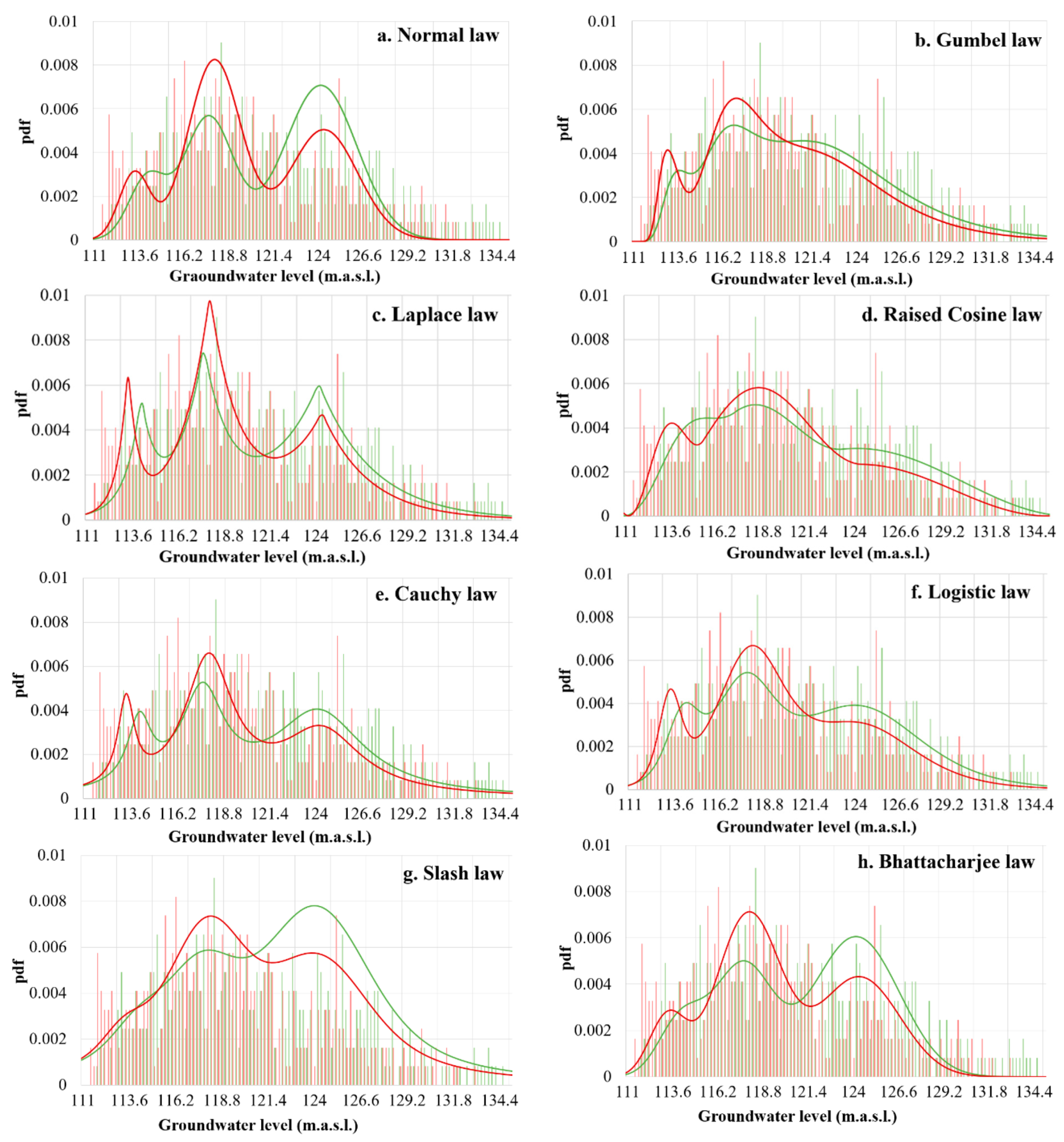
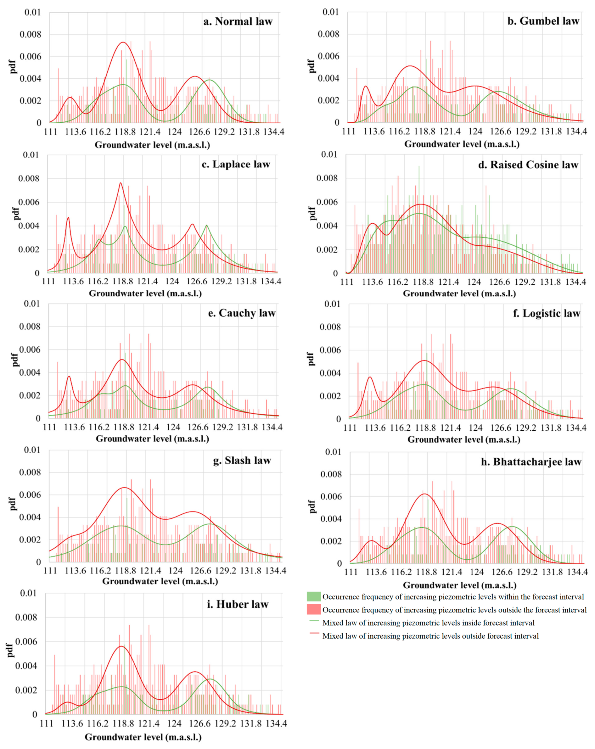
2.5.2. Chosen Probability Density Functions
3. Model Design
3.1. Definition of Subsets for Training Testing, Stop and Cross-Validation
3.2. Choice of the Model and Complexity Selection
4. Results
4.1. Optimal Number of Members in Ensemble Models
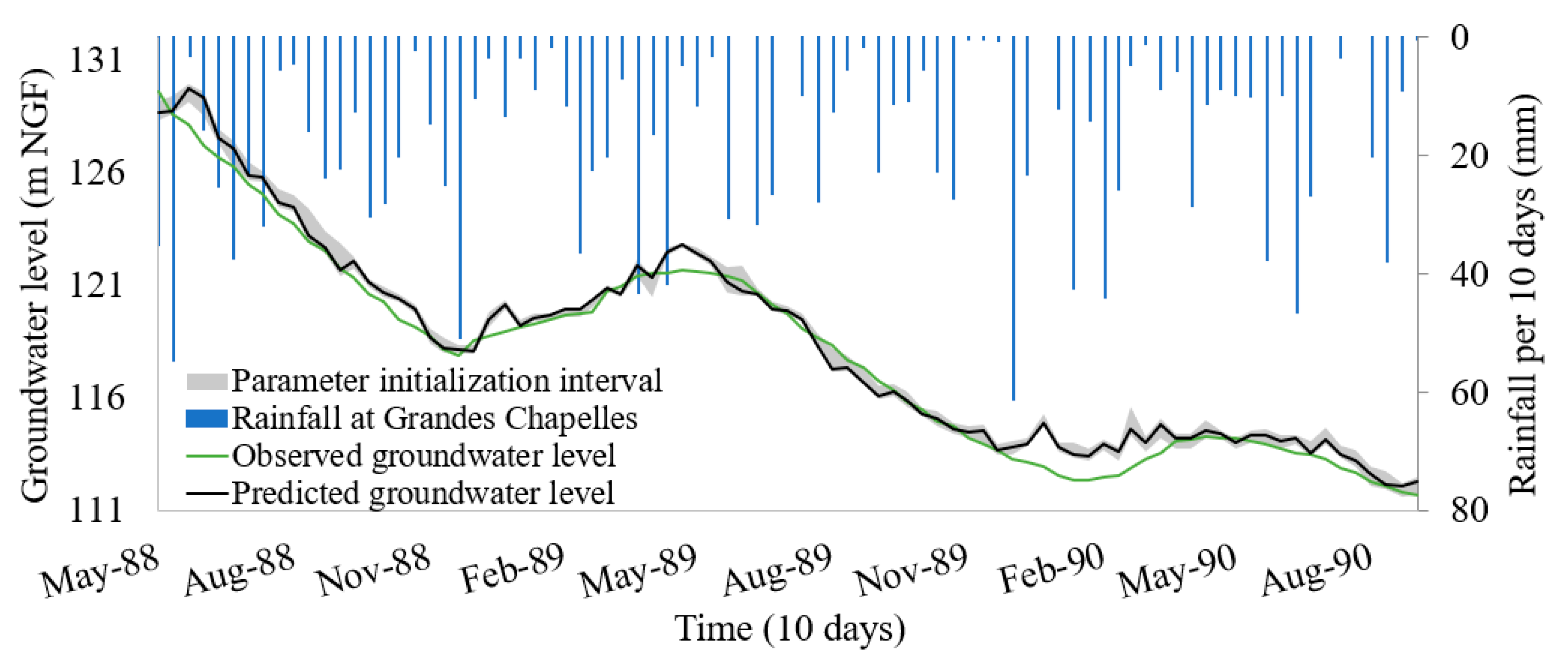
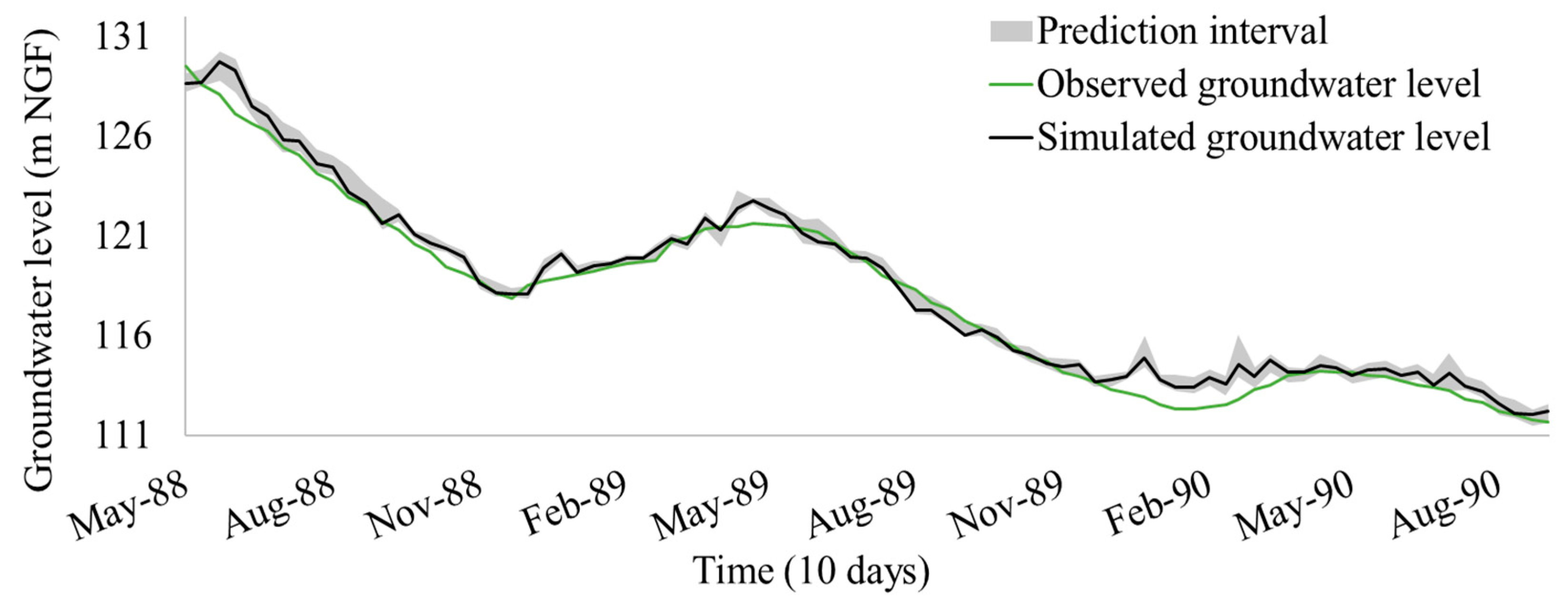
4.2. Prediction Results
4.3. Representation of Uncertainties Caused by the Initialization Parameters
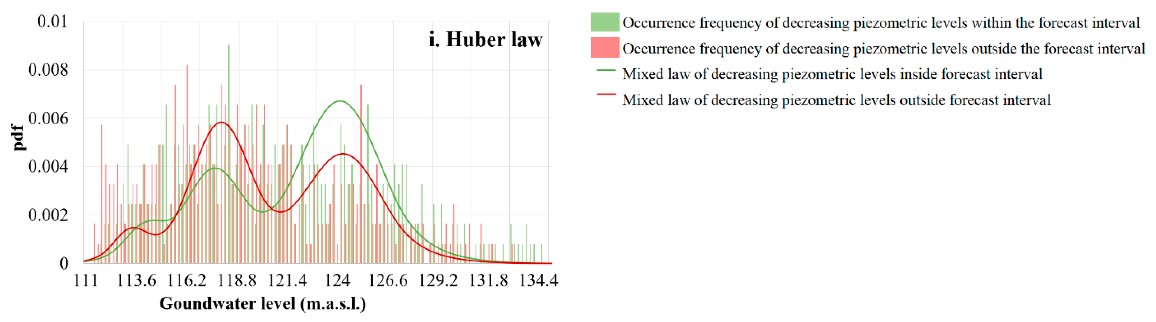
4.3.1. Theoretical Composite pdf for Four Distributions
4.3.2. Error Margins
- -
- It is supposed that the distribution of samples inside a class follows a Normal Distribution,
- -
- When a class contains no sample, for example, the class around 135 m.a.s.l., the error is maximum and is divided into two parts: 50% above 50% underneath the probability.
- -
- When a class contains very few samples (less than three), this class is not considered for rC2 and ME calculations.
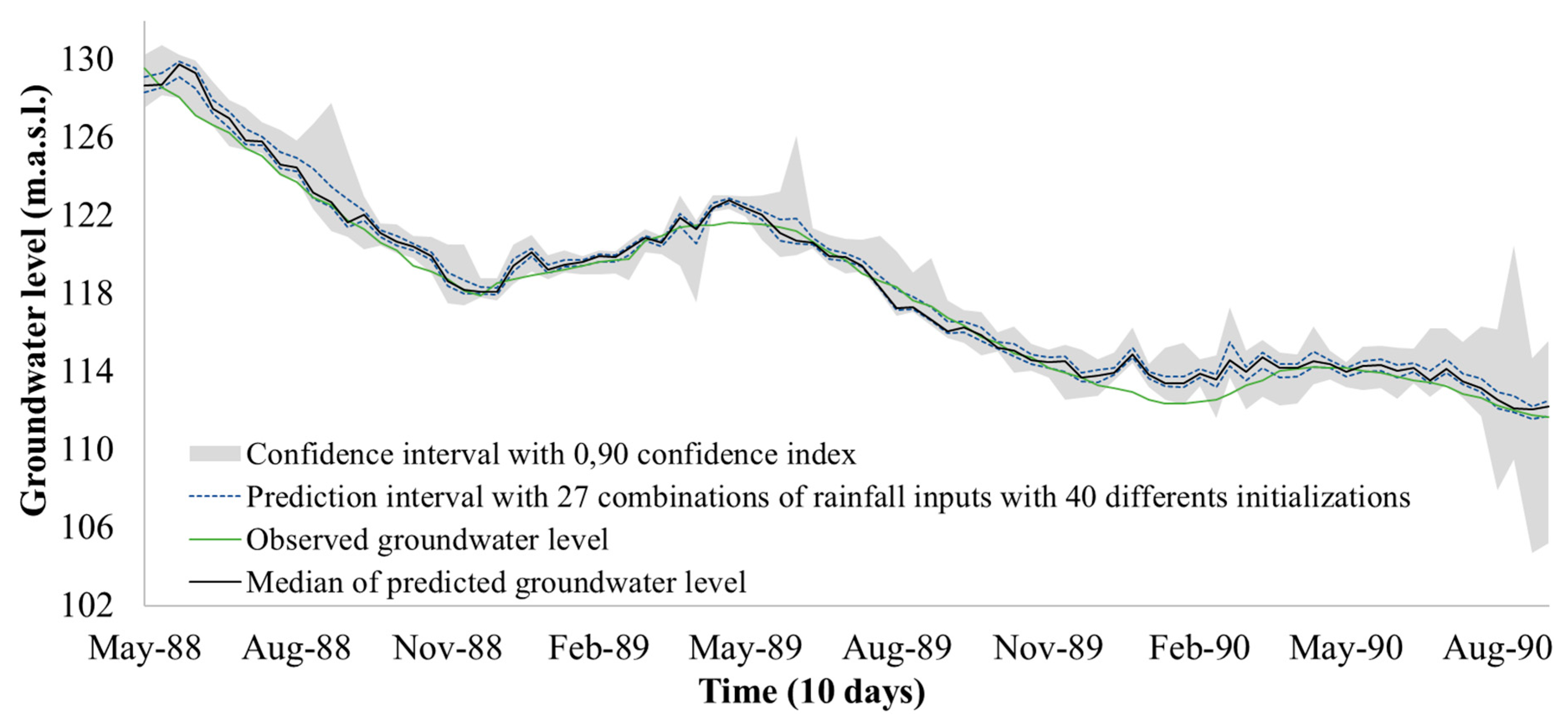
4.4. Determination of Spatial Distribution of Rainfall Uncertainty
4.5. Impact of the Spatial Distribution of Rainfall Uncertainty on the Model of Correctness
4.6. Definition of a Confidence Interval
5. Discussion
5.1. Role of Rain in the Forecast Interval
5.2. Role of the Amount of Data
6. Conclusions
Author Contributions
Funding
Institutional Review Board Statement
Informed Consent Statement
Data Availability Statement
Acknowledgments
Conflicts of Interest
Appendix A

References
- Hartmann, D.L.; Klein Tank, A.M.G.; Rusticucci, M.; Alexander, L.V.; Brönnimann, S.; Charabi, Y.A.-R.; Dentener, F.J.; Dlugokencky, E.J.; Easterling, D.R.; Kaplan, A.; et al. Observations: Atmosphere and Surface. In Climate Change 2013: The Physical Science Basis. Contribution of Working Group I to the Fifth Assessment Report of the Intergovernmental Panel on Climate Change; Cambridge University Press: Cambridge, UK, 2013; Chapter 2; pp. 159–254. [Google Scholar]
- Hornik, K.; Stinchombe, M.; White, H. Multilayer Feedforward Networks are Universal Approximators. Neural Netw. 1989, 2, 359–366. [Google Scholar] [CrossRef]
- Wagener, T.; Montanari, A. Convergence of approaches toward reducing uncertainty in predictions in ungauged basins. Water Resour. Res. 2011, 47. [Google Scholar] [CrossRef] [Green Version]
- Bourgin, F. Comment Quantifier l’incertitude Prédictive en Modélisation Hydrologique? Travail Exploratoire sur un Grand Échantillon de Bassins Versants; AgroParisTech: Paris, France, 2014. [Google Scholar]
- Solomatine, D.P.; Shrestha, D.L. A novel method to estimate model uncertainty using machine learning techniques. Water Resour. Res. 2009, 45, 1–16. [Google Scholar] [CrossRef]
- Biondi, D.; Todini, E. Comparing Hydrological Postprocessors Including Ensemble Predictions into Full Predictive Probability Distribution of Streamflow. Water Resour. Res. 2018, 54, 9860–9882. [Google Scholar] [CrossRef] [Green Version]
- Krzysztofowicz, R. Bayesian theory of probabilistic forecasting via deterministic hydrologic model. Water Resour. Res. 1999, 35, 2739–2750. [Google Scholar] [CrossRef] [Green Version]
- Biondi, D.; Luca, D.L.D. Performance assessment of a Bayesian Forecasting System (BFS) for real-time flood forecasting. J. Hydrol. 2013, 479, 51–63. [Google Scholar] [CrossRef]
- Wu, W.; Dandy, G.C.; Maier, H.R. Protocol for developing ANN models and its application to the assessment of the quality of the ANN model development process in drinking water quality modelling. Environ. Model. Softw. 2014, 54, 108–127. [Google Scholar] [CrossRef]
- Kong-A-Siou, L.; Johannet, A.; Borrell, V.; Pistre, S. Complexity selection of a neural network model for karst flood forecasting: The case of the Lez Basin (southern France). J. Hydrol. 2011, 403, 367–380. [Google Scholar] [CrossRef] [Green Version]
- Stone, M. Cross-Validatory Choice and Assessment of Statistical Predictions (With Discussion). J. R. Stat. Soc. Ser. B 1974, 38, 111–147. [Google Scholar] [CrossRef]
- Sjöberg, J.; Zhang, Q.; Ljung, L.; Benveniste, A.; Delyon, B.; Glorennec, P.-Y.; Hjalmarsson, H.; Juditskys, A. Nonlinear Black-box Modeling in System Identification: A Unified Overview. Automatica 1995, 31, 1691–1724. [Google Scholar] [CrossRef] [Green Version]
- Akil, N.; Artigue, G.; Savary, M.; Johannet, A.; Vinches, M. Quantification of Neural Network Uncertainties on the Hydrogeological Predictions by Probability Density Functions. In Proceedings of the IOP Conference Series: Earth and Environmental Science, Prague, Czech Republic, 9–13 September 2019; p. 10. [Google Scholar]
- Dreyfus, G. Neural Networks, Methodology and Applications; Springer: Berlin, Germany, 2005; p. 509. [Google Scholar]
- Hornik, K. Approximation capabilities of multilayer feedforward networks. Neural Netw. 1991, 4, 251–257. [Google Scholar] [CrossRef]
- Barron, A.R. Approximation bounds for superpositions of a sigmoidal function. In Proceedings of the IEEE International Symposium on Information Theory—Proceedings, San Antonio, TX, USA, 17–22 January 1993; pp. 930–945. [Google Scholar]
- Nerrand, O.; Roussel-Ragot, P.; Personnaz, L.; Dreyfus, G.; Marcos, S. Neural Networks and Nonlinear Adaptive Filtering: Unifying Concepts and New Algorithms. Neural Comput. 1993, 5, 165–199. [Google Scholar] [CrossRef]
- Artigue, G.; Johannet, A.; Borrell, V.; Pistre, S. Flash flood forecasting in poorly gauged basins using neural networks: Case study of the Gardon de Mialet basin (southern France). Nat. Hazards Earth Syst. Sci. 2012, 12, 3307–3324. [Google Scholar] [CrossRef] [Green Version]
- Taver, V.; Johannet, A.; Borrell-Estupina, V.; Pistre, S. Feed-forward vs recurrent neural network models for non-stationarity modelling using data assimilation and adaptivity. Hydrol. Sci. J. 2015, 60, 1242–1265. [Google Scholar] [CrossRef] [Green Version]
- Geman, S.; Bienenstock, E.; Doursat, R. Neural Networks and the Bias/Variance dilemma. Neural Comput. 1992, 4, 1–58. [Google Scholar] [CrossRef]
- Darras, T.; Johannet, A.; Vayssade, B.; Long-a-Siou, L.; Pistre, S. Influence of the Initialization of Multilayer Perceptron for Flash Floods Forecasting: How Designing a Robust Model. In International Work-Conference on Time Series 2014; Springer: Granada, Spain, 2014; p. 13. [Google Scholar]
- Kong-A-Siou, L.; Johannet, A.; Borrell Estupina, V.; Pistre, S. Optimization of the generalization capability for rainfall-runoff modeling by neural networks: The case of the Lez aquifer (southern France). Environ. Earth Sci. 2012, 65, 2365–2375. [Google Scholar] [CrossRef]
- AESN. Fiche de Caractérisation de la ME HG20—Masse d’eau souterraine HG208 “Craie de Champagne Sud et Centre; AESN: Nanterre, France, 2015. [Google Scholar]
- Météo France. Données Publiques—Observations In Situ. Available online: https://donneespubliques.meteofrance.fr/?fond=rubrique&id_rubrique=26 (accessed on 8 September 2020).
- BNPE. Base de données des prélèvements en eau, OPR0000035289. Available online: https://bnpe.eaufrance.fr/acces-donnees/codeOuvrage/OPR0000035289/annee/2014 (accessed on 15 January 2021).
- BNPE. Base de Données des Prélèvements en eau, Vailly (10). Available online: https://bnpe.eaufrance.fr/?q=acces-donnees/codeCommune/10391/annee/2017/etCommunesAdjacentes (accessed on 31 May 2021).
- Stollsteiner, P. Connaissance des Ressources Réellement Disponibles sur L'ensemble des Bassins Versants Crayeux; BRGM: Reims, France, 2013. [Google Scholar]
- Kloppmann, W.; Dever, L.; Edmunds, W.M. Residence time of Chalk groundwaters in the Paris Basin and the North German Basin: A geochemical approach. Appl. Geochem. 1998, 13, 593–606. [Google Scholar] [CrossRef] [Green Version]
- Pinault, J.-L.; Allier, D.; Chabart, M. Prévision des Volumes d’eau Exploitables de 10 Bassins versants en Champagne Crayeuse; BRGM: Reims, France, 2006. [Google Scholar]
- Putot, E.; Verjus, P.; Vernoux, J.F. Qualification des Piézomètres du Réseau de Bassin Seine Normandie en 2005; BRGM: Massy, France, 2006. [Google Scholar]
- IGN. Registre Parcellaire Graphique (RPG): Contours Des Parcelles et Îlots Culturaux et Leur Groupe de Cultures Majoritaire. Available online: https://www.data.gouv.fr/fr/datasets/registre-parcellaire-graphique-rpg-contours-des-parcelles-et-ilots-culturaux-et-leur-groupe-de-cultures-majoritaire/#_ (accessed on 14 September 2020).
- Mangin, A. Pour une meilleure connaissance des systèmes hydrologiques à partir des analyses corrélatoire et spectrale. J. Hydrol. 1984, 67, 25–43. [Google Scholar] [CrossRef]
- Kitanidis, P.K.; Bras, R.L. Real-time forecasting with a conceptual hydrologic model: 2. Applications and results. Water Resour. Res. 1980, 16, 1034–1044. [Google Scholar] [CrossRef]
- Shrestha, D.L.; Solomatine, D.P. Machine learning approaches for estimation of prediction interval for the model output. Neural Netw. 2006, 19, 225–235. [Google Scholar] [CrossRef]
- Khosravi, A.; Nahavandi, S.; Creighton, D. A prediction interval-based approach to determine optimal structures of neural network metamodels. Expert Syst. Appl. 2010, 37, 2377–2387. [Google Scholar] [CrossRef]
- Dempster, A.P.; Laird, N.M.; Rubin, D.B. Maximum Likelihood from Incomplete Data via the EM Algorithm. J. R. Stat. Soc. Ser. B 1977, 39, 1–22. [Google Scholar]
- Benaglia, T.; Chauveau, D.; Hunter, D.R.; Young, D.S. Mixtools: An R Package for Analyzing Finite Mixture Models. J. Stat. Softw. 2009, 32, 29. [Google Scholar] [CrossRef] [Green Version]
- De Moivre, A. The Doctrine of Chances, or, A Method of Calculating the Probability of Events in Play, III ed.; Chelsea Publishing Company: Londres, UK, 1756; p. 368. [Google Scholar]
- Fisher, R.A. On the mathematical foundations of theoretical statistics. Philos. Trans. R. Soc. 1922, 9, 309–368. [Google Scholar]
- Gumbel, E.J. Méthodes graphiques pour l'analyse de débits de crues. Rev. De Stat. Appl. 1957, 5, 77–89. [Google Scholar] [CrossRef] [Green Version]
- Laplace, P.-S. Mémoire sur la probabilité des causes par les évènements. In Œuvres complètes de Laplace; Mémoires de l’Academie Royale des Sciences, Ed.; Divers Savan: Paris, France, 1774; Chapter 6; pp. 621–656. [Google Scholar]
- Rinne, H. Location-Scale Distributions Linear Estimation and Probability Plotting Using MATLAB; Justus Liebig University: Giessen, Allemagne, 2010. [Google Scholar]
- Sinha, R.K. A Thought on Exotic Statistical Distributions. Int. J. Math. Comput. Sci. 2012, 6, 49–52. [Google Scholar]
- Cauchy, A.-L. CALCUL DES PROBABILITÉS—Sur les résultats moyens d’observations de même nature, et sur les résultats les plus probables. In Oeuvres Complètes; Cambridge University Press: Cambridge, UK, 1853; pp. 94–104. [Google Scholar]
- Stigler, S.M. An Historical Note on the Cauchy Distribution; Biometrika Trust: Oxford, UK, 1974; pp. 375–380. [Google Scholar]
- Verhulst, P.F. Recherches mathématiques sur la loi d'accroissement de la population. In Nouveaux mémoires de l'Académie Royale des Sciences et Belles-Lettres de Bruxelles; Nabu Press: Bruxelles, Belgique, 1845; Chapter 18; pp. 1–38. [Google Scholar]
- Rogers, W.H.; Tukey, J.W. Understanding some long-tailed symmetrical distributions. Stat. Neerl. 1972, 26, 211–226. [Google Scholar] [CrossRef]
- Bhattacharjee, G.P.; Pandit, S.N.N.; Mohan, R. Dimensional Chains Involving Rectangular and Normal Error-Distributions. Technometrics 1963, 5, 404–406. [Google Scholar] [CrossRef]
- Huber, P.J. Robust estimation of a location parameter. Ann. Math. Stat. 1964, 35, 73–101. [Google Scholar] [CrossRef]
- Huber, P.J. Robust Statistics; Wiley: Hoboken, NJ, USA, 1981; p. 308. [Google Scholar]
- Levenberg, K. A method for the solution of certain non-linear problems in least squares. Q. Appl. Math. 1944, 2, 164–168. [Google Scholar] [CrossRef] [Green Version]
- Marquardt, D.W. An Algorithm for Least-Squares Estimation of Nonlinear Parameters. J. Soc. Ind. Appl. Math. 1963, 11, 431–441. [Google Scholar] [CrossRef]


| Station Name | Measured Variable | Unit | Time Step | Max Value | Min Value | Median | Average |
|---|---|---|---|---|---|---|---|
| Craie at Vailly (LCV) | Level | m.a.s.l. | 10 days | 134.75 | 109.75 | 119.95 | 120.558 |
| Barbuise at Pouan les Vallées (DBP) | Discharge | m3.s−1 | 10 days | 4.50 | 0.00 | 0.67 | 0.836 |
| Seine at Méry-sur-Seine (DSM) | Discharge | m3.s−1 | 10 days | 182.2 | 5.95 | 25.61 | 35.71 |
| Grandes-Chapelles (RGC) | Rain | mm | 10 days | 131.2 | 0.0 | 15.9 | 19.87 |
| Troyes-Barberey (RTB) | Rain | mm | 10 days | 86.4 | 0.0 | 13.2 | 17.29 |
| Mailly (RMA) | Rain | mm | 10 days | 138.8 | 0.0 | 17.0 | 21.50 |
| Troyes-Barberey (PET) | Potential Evapo-transpiration | mm | 10 days | 64.7 | 0.0 | 19.0 | 21.20 |
| Bassin (I) | Irrigation | m3.ha−1.month−1 | month | 833.9 | 0.6 | 176.0 | 280.1 |
| LCV | ΔLCV | DBP | DSM | RGC | RTB | RMA | PET | I | |
|---|---|---|---|---|---|---|---|---|---|
| LCV | 17 | 6 | 2 | 5 | 21 | 22 | 15 | 12 | 16 |
| ΔLCV | 15 | 4 | −4 | 0 | 1 | 1 | 1 | 4 | 8 |
| DBP | 17 | 1 | 11 | 3 | 2 | 6 | 7 | 9 | 12 |
| DSM | 19 | 4 | 15 | 5 | 1 | 1 | 1 | 3 | 7 |
| RGC | NC | 2 | NC | 3 | 0 | 0 | 0 | 0 | 27 |
| RTB | NC | 2 | NC | 3 | 1 | 1 | 0 | 0 | 27 |
| RMA | NC | 3 | NC | 3 | 0 | 1 | 0 | 0 | 33 |
| PET | 19 | 11 | 16 | 9 | NC | NC | NC | 8 | 4 |
| I | 22 | 14 | 19 | 12 | NC | NC | NC | 11 | 7 |
| Name of pdf Law | Formula | Eq. | References |
|---|---|---|---|
| Normal | (10) | [38,39] | |
| Gumbel | (11) | [40] | |
| Laplace | (12) | [41] | |
| Raised Cosine | (13) | [42,43] | |
| Cauchy | (14) | [44,45] | |
| Logistic | (15) | [46] | |
| Slash | (16) | [47] | |
| Bhattacharjee | (17) | [48] | |
| Huber | (18) | [49,50] |
| 1 | 2 | 3 | 4 | 5 | 6 | 7 | 8 | 9 | 10 | 11 | 12 | 13 | 14 | 15 | Scores |
|---|---|---|---|---|---|---|---|---|---|---|---|---|---|---|---|
| V | T | T | T | T | T | T | T | T | T | T | S | T | T | Te | |
| T | V | T | T | T | T | T | T | T | T | T | S | T | T | Te | |
| T | T | V | T | T | T | T | T | T | T | T | S | T | T | Te | |
| T | T | T | V | T | T | T | T | T | T | T | S | T | T | Te | |
| … | |||||||||||||||
| T | T | T | T | T | T | T | T | T | T | V | S | T | T | Te | |
| T | T | T | T | T | T | T | T | T | T | T | S | V | T | Te | |
| T | T | T | T | T | T | T | T | T | T | T | S | T | V | Te | |
| Median | |||||||||||||||
| Model Element | Selected Hyperparameters | Tested Range Values | ||
|---|---|---|---|---|
| Order | r (LCV) | 3 | (3–6) | (8–14) |
| Exogenous input window-widths | n1 (I) | 8 | (7–10) | |
| n2 (PET) | 12 | (9–12) | (9–12) | |
| n3 (DSM) | 5 | (2–5) | ||
| n4 (DBP) | 5 | (2–5) | (2–5) | |
| n5 (RGC) | 2 | (1–4) | (7–12) | |
| n6 (RTB) | 2 | (1–4) | (7–12) | |
| n7 (RMA) | 3 | (1–4) | (7–12) | |
| Number of hidden neurons | N | 3 | (2–10) | (2–10) |
| Law | Normal | Gumbel | Laplace | Raised Cosine | Cauchy | Logistic | Slash | Bhatta-Charjee | Huber |
|---|---|---|---|---|---|---|---|---|---|
| 0.62 | 0.74 | 0.66 | 0.76 | 0.69 | 0.75 | 0.64 | 0.64 | 0.50 | |
| 0.68 | 0.74 | 0.67 | 0.77 | 0.70 | 0.75 | 0.72 | 0.75 | 0.65 |
| Law | Normal | Gumbel | Laplace | Raised Cosine | Cauchy | Logistic | Slash | Bhatta-Charjee | Huber |
|---|---|---|---|---|---|---|---|---|---|
| 0.43 | 0.41 | 0.47 | 0.44 | 0.45 | 0.44 | 0.43 | 0.43 | 0.42 | |
| 0.52 | 0.54 | 0.54 | 0.66 | 0.55 | 0.61 | 0.63 | 0.57 | 0.52 |
| Law | Normal | Gumbel | Laplace | Raised Cosine | Cauchy | Logistic | Slash | Bhatta-charjee | Huber |
|---|---|---|---|---|---|---|---|---|---|
| 0.15 | 0.04 | 0.24 | 0.19 | 0.25 | 0.24 | 0.22 | 0.16 | 0.20 | |
| 76.3% | 73.7% | 72.4% | 76.3% | 75.0% | 73.7% | 80.3% | 76.3% | 77.6% |
| Law | Normal | Gumbel | Laplace | Raised Cosine | Cauchy | Logistic | Slash | Bhatta-charjee | Huber |
|---|---|---|---|---|---|---|---|---|---|
| 0.02 | 0.21 | 0.16 | 0.21 | 0.23 | 0.23 | 0.30 | 0.28 | 0.27 | |
| 74.4% | 70.3% | 70.3% | 72.5% | 70.3% | 79.1% | 71.4% | 73.6% | 70.3% |
| Groundwater Level Class | Criteria | Laws | |||
|---|---|---|---|---|---|
| Gumbel | Raised Cosine | Logistic | Slash | ||
| Positive Slope | 0.47 | 0.59 | 0.55 | 0.55 | |
| 0.52 | 0.56 | 0.53 | 0.54 | ||
| 0.19 | 0.33 | 0.20 | 0.15 | ||
| 60.5% | 61.8% | 60.5% | 63.2% | ||
| Negative Slope | 0.78 | 0.79 | 0.77 | 0.72 | |
| 0.74 | 0.79 | 0.77 | 0.71 | ||
| 0.52 | 0.41 | 0.49 | 0.47 | ||
| 70.3% | 72.5% | 71.4% | 67.0% | ||
| Confidence Index | CPICP (Train + Test Datasets) | CPICP (Test Set) | CMPI (m) | CMPI (m) (Without Extreme Values) |
|---|---|---|---|---|
| 0.60 | 0.60 | 0.42 | 2.51 | 2.20 |
| 0.65 | 0.65 | 0.45 | 2.80 | 2.45 |
| 0.70 | 0.70 | 0.52 | 3.18 | 2.78 |
| 0.75 | 0.75 | 0.58 | 3.75 | 3.28 |
| 0.80 | 0.81 | 0.62 | 4.66 | 4.08 |
| 0.85 | 0.86 | 0.68 | 6.14 | 5.37 |
| 0.90 | 0.91 | 0.81 | 8.47 | 7.42 |
| 0.95 | 0.95 | 0.94 | 17.44 | 15.27 |
Publisher’s Note: MDPI stays neutral with regard to jurisdictional claims in published maps and institutional affiliations. |
© 2021 by the authors. Licensee MDPI, Basel, Switzerland. This article is an open access article distributed under the terms and conditions of the Creative Commons Attribution (CC BY) license (https://creativecommons.org/licenses/by/4.0/).
Share and Cite
Akil, N.; Artigue, G.; Savary, M.; Johannet, A.; Vinches, M. Uncertainty Estimation in Hydrogeological Forecasting with Neural Networks: Impact of Spatial Distribution of Rainfalls and Random Initialization of the Model. Water 2021, 13, 1690. https://doi.org/10.3390/w13121690
Akil N, Artigue G, Savary M, Johannet A, Vinches M. Uncertainty Estimation in Hydrogeological Forecasting with Neural Networks: Impact of Spatial Distribution of Rainfalls and Random Initialization of the Model. Water. 2021; 13(12):1690. https://doi.org/10.3390/w13121690
Chicago/Turabian StyleAkil, Nicolas, Guillaume Artigue, Michaël Savary, Anne Johannet, and Marc Vinches. 2021. "Uncertainty Estimation in Hydrogeological Forecasting with Neural Networks: Impact of Spatial Distribution of Rainfalls and Random Initialization of the Model" Water 13, no. 12: 1690. https://doi.org/10.3390/w13121690