Article

NutSpaFHy—A Distributed Nutrient Balance Model to Predict Nutrient Export from Managed Boreal Headwater Catchments

by
Annamari (Ari) Lauren
1,*,
Mingfu Guan
2,
Aura Salmivaara
3,†,
Antti Leinonen
4,†,
Marjo Palviainen
5,† and
Samuli Launiainen
3
1
Faculty of Science and Forestry, Joensuu Campus, School of Forest Sciences, University of Eastern Finland, PO Box 111, Yliopistokatu 7, FI-80101 Joensuu, Finland
2
Department of Civil Engineering, University of Hong Kong, Hong Kong, China
3
Natural Resources Institute Finland (Luke), Latokartanonkaari 9, FI-00790 Helsinki, Finland
4
Finnish Forest Centre, Kauppakatu 25 A, FI-87100 Kajaani, Finland
5
Department of Forest Sciences, University of Helsinki, PO Box 27, FI-00014 Helsinki, Finland
*
Author to whom correspondence should be addressed.
These authors contributed equally to this work.
Forests 2021, 12(6), 808; https://doi.org/10.3390/f12060808
Submission received: 10 May 2021 / Revised: 6 June 2021 / Accepted: 12 June 2021 / Published: 18 June 2021
(This article belongs to the Special Issue Forest Management, Hydrology and Biogeochemistry Modelling)

Abstract

:
Responsible forest management requires accounting for adverse environmental effects, such as increased nutrient export to water courses. We constructed a spatially-distributed nutrient balance model NutSpaFHy that extends the hydrological model SpaFHy by introducing a grid-based nutrient balance sub-model and a conceptual solute transport routine to approximate total nitrogen (N) and phosphorus (P) export to streams. NutSpaFHy uses openly-available Multi-Source National Forest Inventory data, soil maps, topographic databases, location of water bodies, and meteorological variables as input, and computes nutrient processes in monthly time-steps. NutSpaFHy contains two calibrated parameters both for N and P, which were optimized against measured N and P concentrations in runoff from twelve forested catchments distributed across Finland. NutSpaFHy was independently tested against six catchments. The model produced realistic nutrient exports. For one catchment, we simulated 25 scenarios, where clear-cuts were located differently with respect to distance to water body, location on mineral or peat soil, and on sites with different fertility. Results indicate that NutSpaFHy can be used to identify current and future nutrient export hot spots, allowing comparison of logging scenarios with variable harvesting area, location and harvest techniques, and to identify acceptable scenarios that preserve the wood supply whilst maintaining acceptable level of nutrient export.

1. Introduction

Responsible forest management requires balancing between the economic gains and adverse environmental effects of the production [1]. In Nordic and Baltic countries, forestry has a significant role in national and regional economies but also risks adverse environmental effects. Forest management operations increase nutrient exports to water courses deteriorating water quality especially in headwater streams and lakes [2,3,4,5], but forestry is also a significant source of nutrient load to the Baltic sea [2]. Forest harvesting increases nutrient export through combined hydrological and biogeochemical responses. After the removal of trees, runoff increases [6] and nutrient release exceeds the uptake resulting in increased nutrient transport to water courses [7].
Numerous experimental studies have quantified the effects of forest management on the water quality and nutrient export in headwater catchments [2,4,7,8]. The results are, however, difficult to generalize because nutrient export is affected by several compounding factors. These include, for instance, site fertility and soil properties [9,10,11], topography [12], tree species and ground vegetation [13,14], varying climate and weather conditions [2] and atmospheric deposition [10,15]. Moreover, the size of the harvested area in relation to the size of the catchment, the distance from the receiving water body [4,9,16], dimensions of the buffer zones [8,9], and the intensity and timing of harvesting affect the magnitude and dynamics of nutrient release and export from the terrestrial system to streams.
Novel planning tools are needed to detect areas where forest management may cause increased nutrient leaching, and to choose suitable management practices and water protection methods, such as buffer zones. Such planning tools are currently not available, although different alternatives to estimate nutrient loads from forest management exist. The simplest one is the specific export approach [17,18,19] that computes nutrient loading as a product of managed areas and static export coefficients, which are based on a small number of plot or catchment-scale experiments [17]. As the method lacks spatial context and ignores hydrometeorological variablity altogether, its use is limited to coarse estimates of regional loading and its attribution to different sources. On the other end of the spectrum, there are sophisticated process models on coupled hydrological and nutrient cycle and nutrient transport within stands and catchments [8,20,21]. These models describe water and solute transport and nutrient dynamics at different levels of complexity; there is, however, often no satisfactory means to describe and independently parameterize different processes. As a result, a large number (from tens to hundred) of parameters are commonly calibrated against only a few datasets such as stream runoff and nutrient concentrations, which leads to problem of model equifinality [22] and limits the use of complex models to intensively monitored research catchments.
In the boreal forests, considerable differences in water fluxes, soil moisture and site fertility emerge at scales of kilometres to meters [23,24] following the topographic relief [25]. The water and nutrient availability are the decisive factors for determining forest productivity and the scale of response under forest management operations [26]. Based on this rationale, topographic wetness indices are used to identify wet areas in the landscape, improve multi-criteria forest planning [26] and optimize location and dimensions of buffer zones [27]. While already being implemented in forest planning systems in Finland and Sweden [28,29] the approach remains as a static and qualitative rank of moisture conditions within the catchment.
In forest management planning, the traditional scale has been the individual stand or set of stands managed by a single forest owner. However, from a water quality perspective, a catchment forms the basic unit to quantify the impacts of forestry as water and nutrients released from a site are transported to the downstream watercourse. To bridge these two scales, we developed a distributed nutrient balance and transport model, NutSpaFHy. It extends the recently-proposed Spatial Forest Hydrology model (SpaFHy, [30]), and is designed as a robust and practically applicable tool to quantify nutrient export from managed forested catchments. We test the model’s predictive capability against measured streamwater nitrogen (N) and phosphorus (P) concentrations and export loads at 18 headwater catchments across Finland. After testing, we demonstrate the model in a practical forest planning at a single catchment. We analyzed how location, extent and intensity of forest harvesting affects catchment-level nutrient export and discuss the practical implications of our approach. As NutSpaFHy uses only openly available data as input, and contains only four calibrated parameters, it it is designed to be applicable for whole Finland and extendable to other Nordic and Baltic countries.

2. Materials and Methods
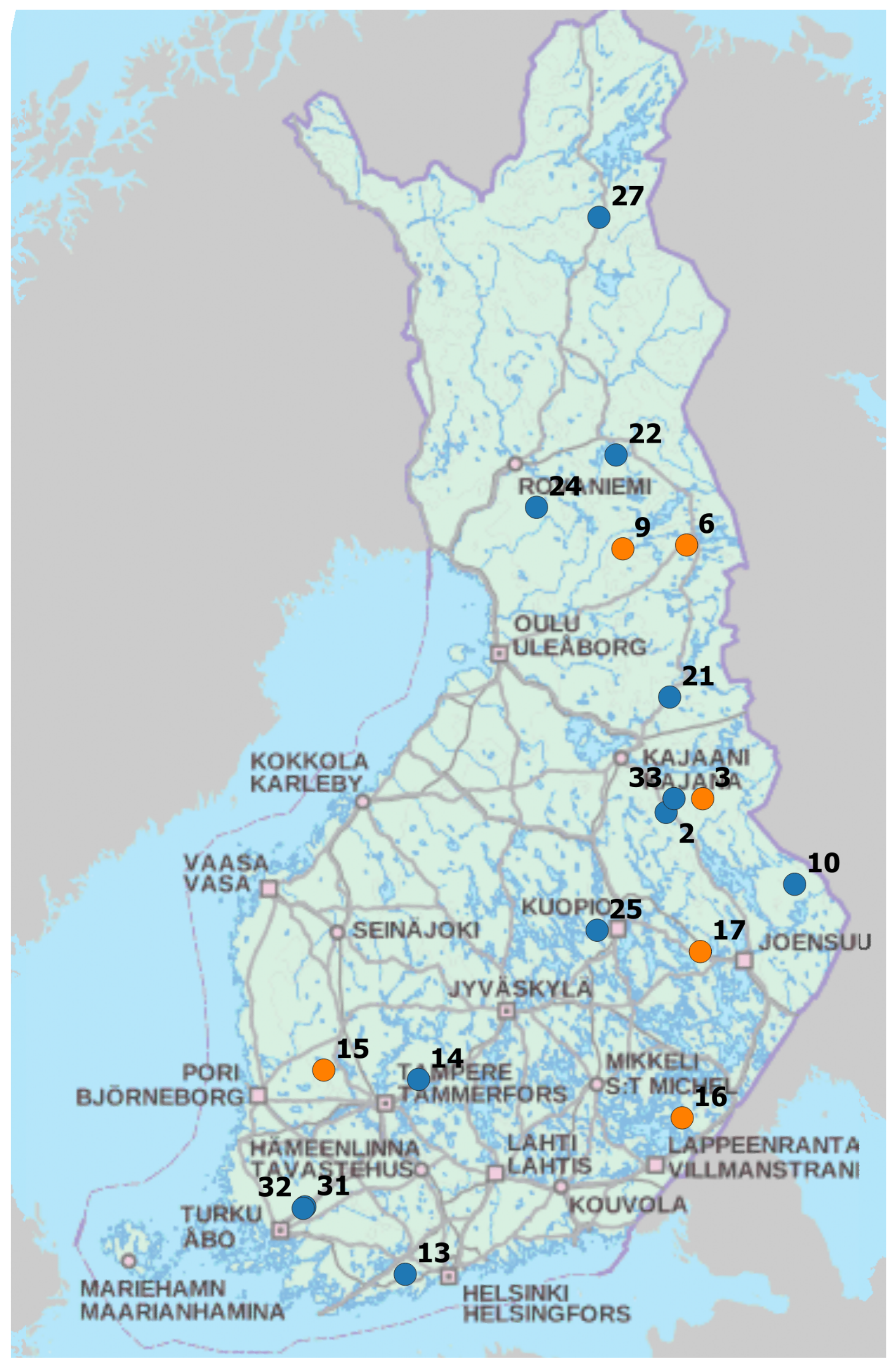
2.1. Field Data

We used data from 18 forest-dominated headwater catchments covering a large geographical area across Finland (Figure 1). Twelve of the catchments were used for model calibration and six as independent test catchments. The area of the catchments ranged from 31 to 1966 ha (Table 1). Five of the catchments were pristine or outside forest management, while 13 were under normal forest management, which typically includes growing of even aged semi-natural stands treated with thinnings and having rotation time from 70 to 120 years. The dominant tree species in the catchment were Scots pine (Pinus sylvestris L.) and Norway spruce (Picea abies Karst.) and the catchment mean stand volume varied between 25 and 166 m3 ha−1. The distribution of site fertility classes in peatland and upland sites are presented in Table A1.
Runoff at catchment outlets was continuously measured from 2014 to 2016 using the V-notch weirs equipped with automatic water level loggers. On average, 20 water samples (data available: https://metsainfo.luke.fi/fi/vesistokuormitukset (accessed on 6 June 2021)) were collected per year and total nitrogen (N) and total phosphorus (P) were determined at certified laboratories using accredited methods (SFS-EN 45001:1990, SFS-EN ISO/IEC 17025:2000, SFS-EN ISO/IEC 17025:2005) [31].
Daily runoff and linearly interpolated concentration time-series were used to calculate the monthly and annual export loads.

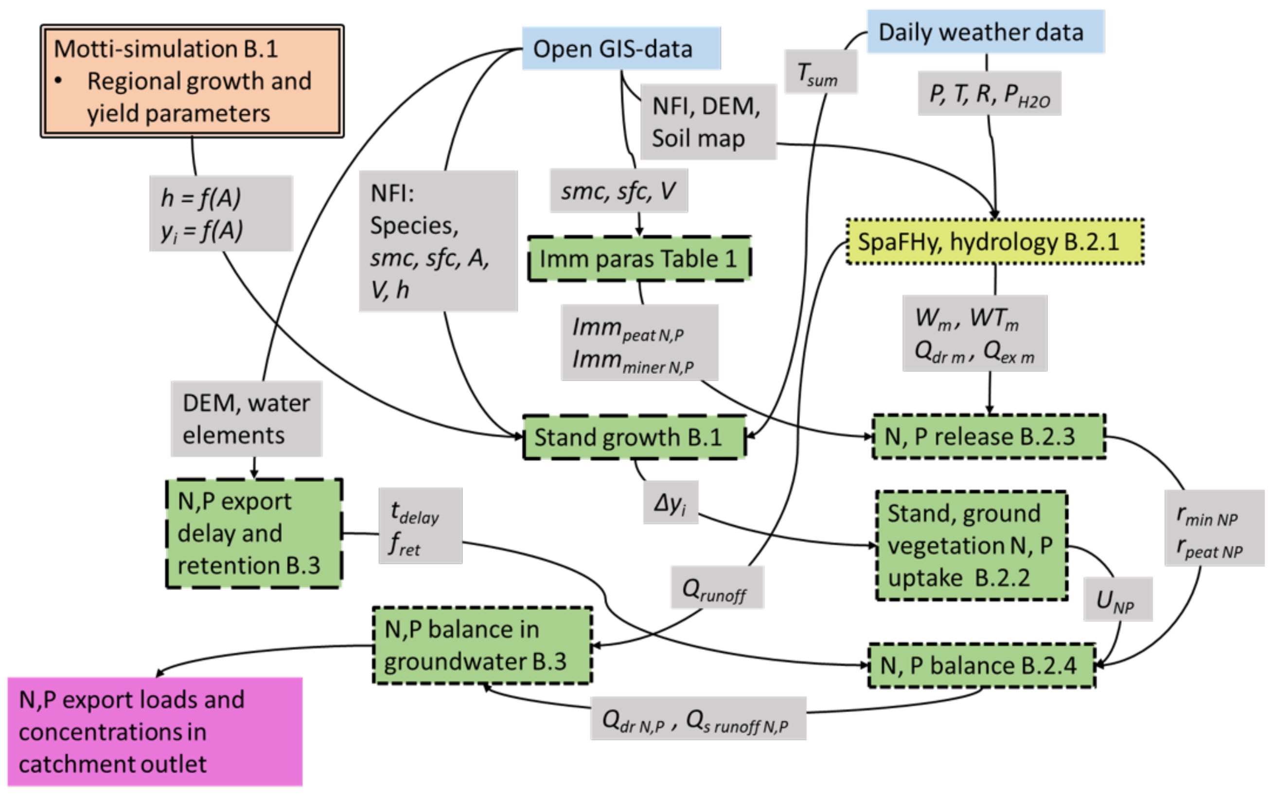
2.2. Model Description

NutSpaFHy is a spatially-distributed nutrient balance model, which extends the hydrological model SpaFHy [30] by introducing grid-based nutrient balance sub-model and a conceptual solute transport routine to approximate total N and P export load to streams (Figure 2). A detailed description of the model is provided in the Appendices.
The model domain consists of a rectangular grid (cell size 16 m) that is initialized using open-source GIS data available throughout the Finland [30]. These include the Multi-source National Forest Inventory (MNFI) data for initial forest structure, soil maps and topographic databases for determining soil type (fine, medium or coarse mineral soils and peatlands) and permanent water elements to locate streams and water bodies. The digital elevation model (DEM) is used to compute local slope, topographic wetness index (TWI) [30,32] and flowpath distances from a grid cell to the nearest stream. Basic daily meteorological data (global radiation, air temperature, humidity and precipitation rate) are used to drive the SpaFHy-model, which produces daily water table ( W T ), root layer water content (W), water flux from root layer to deeper soil ( Q d r ), water flux to root layer from below ( Q e x ), and runoff ( Q r u n o f f ). For NutSpaFHy, the water fluxes and state variables are further aggregated to monthly values. Prior to the NutSpaFHy simulation, a database of development parameters for stand height and yield are computed using Motti-simulator [33]. We treat separately growth and yield of Scots pine (Pinus sylvestris L.) and Norway spruce (Picea abies Karst.) growing on peatland and mineral soil sites in site fertility classes ( s f c ) 2, 3 and 4 (growth decreases with increasing site fertility class, [34]). The initial state of the forest stand in each grid cell is defined by the MNFI data that contains information for the main tree species ( s p e ), s f c and site main class ( s m c , peat/mineral) and the mean stand height ( h g ), volume (V) and age (A). Thereafter, the stand growth follows the development parameters and Equations (A1) and (A2). The growth rate is adjusted according to the annual temperature sum, which incorporates a simple dependency between the growth performance and weather conditions (A13). The growth of stand determines the net nutrient uptake as described by Palviainen and Finér [13] (Equation (A7)). To obtain the gross nutrient uptake we have to add the nutrient uptake by ground vegetation, and the nutrients that are lost in the litter fall as described in Laurén et al. [35]. The total monthly uptake of N and P ( N u p , P u p ) were given as input to soil nutrient balance module.
Decomposition of organic matter in mineral soils and peatlands is described using empirical equations presented by Pumpanen et al. [36] and Ojanen et al. [37], respectively. We use monthly mean air temperature, W m and W T m as drivers of decomposition rate (Appendix B.2.3). During decomposition, a fraction of the released N and P is immobilized to microbe biomass (Equations (A16) and (A20)) as in [35]. Immobilization parameter ( I m m p e a t N P and I m m m i n e r N P ) values in NutSpaFHy were first calibrated using 12 catchments (see Section 2.3), and then a regression model was built to predict these parameters from the catchment properties. The net release of N and P ( r m i n N P , r p e a t N P ) were given as input to nutrient balance module.
The nutrient balance module keeps an account of the total nutrient storage and nutrient concentration in the root layer. At each timestep, the nutrient storage is updated accounting for the nutrient release and uptake and nutrient concentration in the liquid water ( W m ) in the root layer is computed. Using the monthly mean nutrient concentrations and monthly cumulative drainage ( Q d r m ) and surface runoff ( Q e x m ), we calculate the respective nutrient fluxes to groundwater ( Q d r N P ) and as a form of surface runoff ( Q e x N P ).
The nutrient transport via groundwater flow from a grid cell to the receiving water body is delayed by the residence time ( t d e l a y , in months), and reduced by an empirical retention factor that depends on the grid-point distance to the receiving water body [38] (Appendix B.3). The t d e l a y is computed for each grid cell using the slope and distance to the receiving water body. The resulting variable, Q d r N P d e l a y e d , represents the input to the groundwater nutrient storage. The output from the groundwater nutrient storage is nutrient flux with runoff. Nutrients in the surface runoff are transported to the receiving water body without a time delay and no retention processes are considered. The total nutrient flux at the catchment outlet is the sum of the groundwater and surface runoff transport from all grid cells.

2.3. Calibration

Nutrient export load is strongly dominated by runoff, which is modeled using SpaFHy. The hydrological predictions (runoff, evapotranspiration, snow and soil water storage) of SpaFHy have been thoroughly tested against the observed data in [30]. To calibrate the new processes in NutSpaFHy, the monthly mean observed N ( c N o b s ) and P concentrations ( c P o b s ) in the stream water from the twelve catchments were used (Figure 1, Table 1). Optimization was done separately for N and P as there is no interaction between them in the model. For both N and P we had two calibrated parameters, the immobilization factors for mineral and peat soils ( i m m N p e a t , i m m N m i n e r and i m m P p e a t , i m m P m i n e r ). Catchments were calibrated individually in a process, where, in each iteration of the optimization, the observed monthly concentrations were compared to the predicted monthly concentrations using regression through the origin (Equation (1)).
c o b s m = s c p r e d m + ε m ,
where c o b s m was the observed concentration of N and P in month m, c p r e d m was the predicted concentration of N and P for month m, and s is a slope parameter, and ε m is the residual term for month m with expectation value of zero. When s equals to one, NutSpaFHy predicts the nutrient concentration with no bias. Thus, the minimized target variable in the optimization was (s− 1)2. Initial values for all calibrated immobilization parameters was set to 0.9, and the valid range was for the parameter values was set to [0.5, 1.0]. The optimization was conducted with minimize function in scipy.optimize-package in Python 3.7.
To support the model use for ungauged catchments, we investigated whether the immobilization parameters ( i m m N p e a t , i m m N m i n e r and i m m P p e a t , i m m P m i n e r ) can be predicted from catchment characteristics. Using the calibration catchments, we predicted the optimized immobilization parameter values and the catchment characteristics in linear step-wise regression. The backward step-wise regression drops the start from the full model and drops the weakest explaining variables until the model is not improved anymore. Forward stepwise regression starts with a single explanatory variable and adds variables until no improvement is achieved. The used olsrr package in R applies a combination of backward and forward regression analysis. (Table 1 and Table A1, Appendix A).

2.4. Model Testing

The NutSpaFHy model was tested against independent data from six catchments (Figure 1, Table 1). The immobilization parameters were predicted from the catchment characteristics and the root mean square error of the modeled immobilization parameter was used to create 95% confidence intervals for the nutrient concentration and export load predictions (Appendix A). The simulated monthly and annual concentrations and export loads with their confidence intervals were compared to observations.

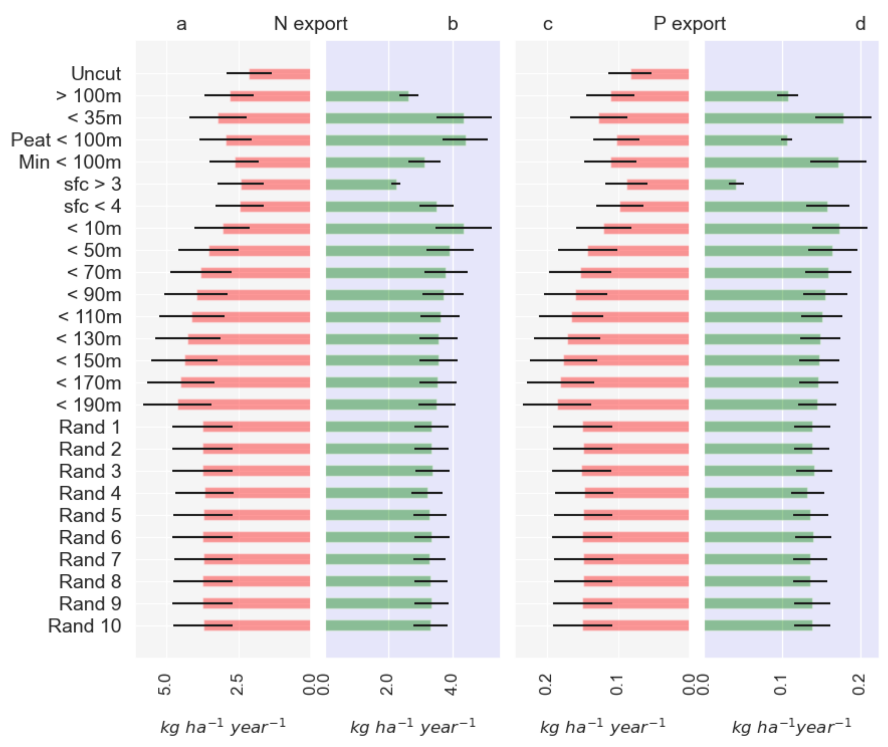
2.5. Application to Clear-Cut Scenario

To test the NutSpaFHy in realistic forest planning situations, we simulated alternative harvesting operations at catchment 2. We compare N and P export loads from 25 alternative clear-cut scenarios to a reference scenario (uncut) where no management was done (Table 2). To follow common forest management practice, we applied clear-cut only at grid cells where the stand volume exceeded 100 m3 ha−1. The scenarios contained alternative harvest regimes, where similar size clear-cut area was located close and far away from the water (<35 m, >100 m), where similar total tree volume was harvested from peat and mineral soils (Peat < 100 m, Min < 100 m), and where total volume was harvested from low fertility ( s f c 4,5,6) vs. high fertility sites ( s f c 1,2,3). In addition, we located clear-cuts extending from stream to 10 ...190 m distance (<10 m ...<190 m), and finally we calculated 10 scenarios, where the clear-cuts with same harvested total volume were randomly located around the catchments (Rand 1 ...10).
The results were expressed both as mean annual export loads (per unit catchment area) during the first 10 years after harvesting, and as specific export loads, where the increase of export load compared to the reference scenario was divided by the fraction of the harvested area from the total catchment area. We selected Catchment 2 for this analysis because it allowed the compilation of versatile management scenarios due to the high mean stand volume distributed quite evenly on both mineral soils and peatlands. These kinds of catchments are prone to high nutrient export loads under intensive forest management.

3. Results

3.1. Model Calibration and Immobilization Parameters

The mean (and range) values for i m m N p e a t , i m m N m i n , i m m P p e a t , i m m N m i n were 0.88 (0.79–0.94), 0.92 (0.84–0.96), 0.92 (0.78–0.97), 0.92 (0.83–0.98), respectively. The N immobilization parameters were found to depend on catchment characteristics, whereas P immobilization was best explained using the mere average over the calibration catchments (Table 3). N immobilization in peat soils increased with an increasing proportion of coniferous tree volume from the total tree volume in the catchment, and decreased with an increasing share of bogs (Appendix A). N immobilization in the mineral soils was increased by the share of low-fertility mineral soils in the catchment.

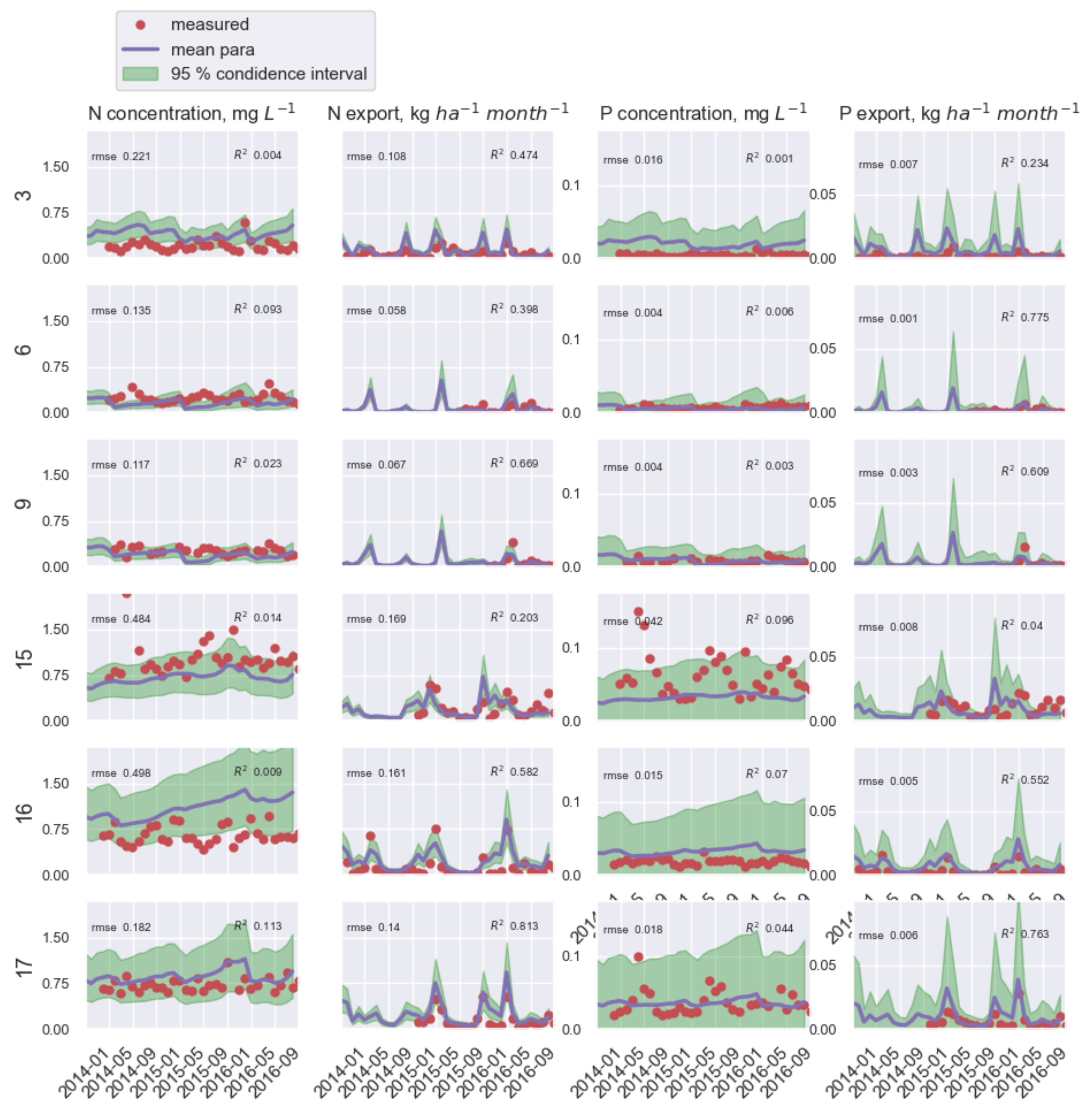
3.2. N and P Concentration and Export Load

The highest monthly export loads of N and P typically emerge during the spring floods, which were well captured by NutSpaFHy (Figure 3 and Figure 4). For the calibration catchments, both the mean concentration and the range of seasonal concentration variation were rather well-captured, especially when the immobilization parameters were calibrated for the specific catchment (Figure 3). However, the timing of the concentration fluctuation was rather poorly predicted. As expected, the model performance decreased when parameters were predicted from catchment characteristics without calibration (Figure 3 and Figure 4). However, in most cases the range of seasonal concentration variation was still rather well as the observed concentrations fit within the model confidence intervals. According to R 2 and R M S E the export loads were better predicted than the concentrations.
The observed annual N export varied from 0.5 to 5 kg ha−1 year−1, and the P export from 0.1 to 0.25 kg ha−1 year−1 (Figure 5). For the test catchments, NutSpaFHy slightly overestimated the annual export loads both for N and P, whereas the annual N concentrations were remarkably well predicted (Figure 5).

3.3. NutSpaFHy Application

To test the NutSpaFHy in realistic forest planning situations, we compared N and P export loads from alternative clear-cut scenarios to a reference scenario (uncut) where no management was done (Table 2). In the uncut scenario, the N and P export were 2.0 and 0.08 kg ha−1 year−1, respectively (Figure 6). Locating a similar size of clear-cut area close to receiving water body (scenario < 35 m) resulted in considerably higher specific N and P export loads than clear-cuts located further away (>100 m) (Figure 6b,d). Harvesting similar tree volume close to the waterbody from peatlands (scenario Peat < 100 m) resulted in higher specific N export, but lower P load than harvesting from mineral soils (Min < 100 m). Clear-cuts in fertile sites ( s f c 1,2,3) led to clearly higher specific exports than in lower-fertility sites ( s f c 3,4,5). Scenarios <10 m ...<190 m describe a situation where the clear-cut area is extended gradually from close to water body towards further-away locations. The total export load (Figure 6a,c) increased with increasing clear-cut area and harvested volume (Table 2), but the specific export decreased when including harvests from further-away grid cells (Figure 6b,d). Results from Rand 1 ...Rand 10 indicate low variability in export loads when half of the catchment area was clear-cut from randomly selected grid-cells.

4. Discussion

4.1. Model Requirements

We built a distributed nutrient balance model NutSpaFHy to simulate forest harvesting impacts on N and P export to watercourses at forested headwater catchments. NutSpaFHy is aimed as a robust and practically applicable tool to assist forest management planning, and thus the model development was guided to meet the following requirements: (1) Modular structure to allow future development; (2) Use only open data for model calibration and applications; (3) Produce realistic nutrient exports in a versatile stand, site and soil combinations; (4) Describe how nutrient export depends on spatial harvesting patterns in the catchment; (5) Respond to climate gradient across Finland, as well as on seasonal and inter-annual variability of meteorological conditions; (6) Have a low number of calibrated parameters to be applicable outside specific research catchments. Moreover, the model code must be distributed under open-source license to stimulate its use and future development.
Meeting the above constraints is challenging, as they mean prioritizing data availability and model applicability over detailed descriptions of biogeochemical and hydrological processes. Thus, the structure of NutSpaFHy reflects balancing between the practical demands and constraints, and the scientific rigor to present the processes regulating nutrient release and transport in boreal ecosystems. Most importantly, we included only the main nutrient in- and outflows, storages, and transport mechanisms in the model, and focused especially on describing those processes and fluxes that are directly affected by forest management practices.

4.2. Evaluation of Model Structure

NutSpaFHy consists of several modules (Figure 2). The hydrological model SpaFHy has been rigorously tested and successfully applied for a large range of different catchments [30]. Based on open data, SpaFHy is particularly good in describing daily grid-cell water fluxes and catchment runoff in heterogeneous catchments. In SpaFHy, grid-cell hydrology responds to local stand characteristics and can well describe the response of these fluxes to leaf-area and species composition changes due to forest management [30]. Drainage from the root zone or return flow from the groundwater link the grid-cell water balance to catchment-level groundwater module. The latter is, however, described using the classical Topmodel-approach [39] that does not explicitly account for water movement from a grid cell to another. Therefore, we created a separate nutrient export module to account for the delay and retention during the export.
Nutrient release in organic matter decomposition and atmospheric bulk deposition are the largest inputs of N and P to soil water [8], whereas the largest outputs are nutrient uptake by stand [13], ground vegetation [14] and soil microbes [40]. In contrast, nitrification, denitrification and N2O emissions are considerably smaller fluxes and omitted from NutSpaFHy as they are difficult to describe and parameterize at the relevant spatiotemporal scales using available data. As organic fractions of N and P dominate in the export loads in boreal forested catchments [18,41], we accounted only for total dissolved nutrients that include both inorganic and organic forms of N and P. This considerably simplifies the model structure, and it is the total nutrient export which determines the water quality because organic N and P are eventually mineralized or photochemically degraded in the water courses [42,43].
Microbial immobilization is an important biochemical nutrient flux in soils [40], and it has been considered to be the primary process affecting especially N leaching [44]. We calibrated N and P immobilization parameters against the observed N and P concentrations in the runoff water. The mean values for all the four immobilization parameters were close to 0.9, which equals the value used in the decompostion—the nutrient dynamics model Romul [45] for early-stage decomposition. A high immobilization rate is expected because organic matter C/N ratio is typically high in boreal soils [46]. Modeling of stream N concentrations was slightly more consistent than P, and the i m m N values could be reasonably well predicted from the catchment properties (Table 3). It is widely known that accurate modeling of P dynamics in terrestrial ecosystems is difficult [47,48] and requires data that is not available at spatial scales relevant for distributed catchment models. This is especially because processes controlling P kinetics and transport are closely related to biogeochemical and hydrological processes such as soil redox conditions and the presence of iron and aluminum in soil [49,50,51].
The growth of trees and understory vegetation is the primary driver for nutrient uptake. The initial state of the forest stand in NutSpaFHy is described based on reasonably accurate gridded forest data [52]. The stand growth onwards from the initial state is described using statistical growth curve parameterized for each site type a priori, and the monthly nutrient uptake follows the prevailing weather conditions in a simple way. Furthermore, the development of understory vegetation follows the stand development. It is clear that the tree stand development is too simplistic to make NutSpaFHy a growth and yield simulator; however, the current stand description is flexible enough to produce reasonable estimates for nutrient uptake for versatile sites, stands and weather conditions. Forest harvesting, such as thinning or clear-cutting affect the nutrient balance through decreasing the nutrient uptake and increasing runoff, and consequently more nutrients are leached. Decomposition models in NutSpaFHy [36,37] are robust empirical models which are responsive to prevailing temperature, soil moisture, fertility and forest stand volume. However, the current versions of the decomposition models do not include the input of logging residues into the soil and the consequent increase in the organic matter decay. A future development of NutSpaFHy should include a decomposition model that accounts for the organic matter mass balance in the soil.
The time delay and the nutrient retention during the transport are the most important catchment-level factors that regulate the dynamics and magnitude of nutrient load. The time delay and the nutrient retention can be computed in physically-based solute transport models [8,53,54], where diffusion-advection-dispersion equation is solved in two or three dimensions. These models are computationally very demanding and the parameterization requires detailed soil data that is not available outside of research areas. In NutSpaFHy, we used pre-calculated residence time to describe the time delay and an empirical model to account for the nutrient retention. This approach is simplistic, but computationally efficient. It is unlikely that this approach is capable of producing daily nutrient export dynamics; however, in forest planning the export loads become meaningful only in much longer (i.e., annual and decadal) time-scales.

4.3. Model Performance at Study Catchments

In the experimental datasets, we had catchments with different soil types and fertility distributions, climatic conditions, management history and a large range of stand properties. NutSpaFHy was able to produce realistic estimates for seasonal dynamics of N and P export (Figure 3 and Figure 4) and mean annual concentrations and export loads (Figure 5). However, the timing in monthly concentrations was more inaccurate, probably because of the simplified computation of residence time and nutrient retention (Appendix B.3). The time scale in forest management planning is, however from years to decades, and therefore the mismatch in monthly concentrations is not detrimental.

4.4. Nutrient Export from Different Harvesting Scenarios

The NutSpaFHy was tested for different harvesting scenarios at a single catchment. The model predicted higher export loads from harvests that were located close to streams than from those located further away. This is consistent with several field studies showing that uncut buffer zones between the clear-cut and the stream can efficiently reduce nutrient loading to water courses [8,9,55]. Moreover, NutSpaFHy predicts higher specific N export loads from peatland than from mineral soil clear-cuts, which has been documented in several field studies [2,5,56]. In contrast, higher specific P loads were detected from mineral soil than peatland clear-cuts (Figure 6). This most likely reflects the relation between the calibrated i m m P p e a t and i m m P m i n raising from the calibration data, which contained both undrained and drained peatlands. Finér et al. [2] used partly same dataset than us, and found that P export load increased for soil types in the following order: undrained peatlands < mineral soils < drained peatlands. Both drained and undrained peatland grid-cells were treated similarly in our calibration procedure, which may have resulted in lower modeled specific P export loads for peatlands than mineral soils.
According to the clear-cut scenarios, the nutrient export from harvests on fertile sites was higher than that from low fertility site clear-cuts. This reflects primarily differences in the quality and nutrient concentrations in the organic matter, which enables faster decomposition and higher nutrient release from the fertile sites [57,58,59,60].

4.5. Potential for Forest Management Planning

Implementation of the Water Framework Directive (WFD) in commercial forestry has raised a need to quantify the impact of various harvesting scenarios on nutrient exports from catchments. Accounting for the landscape heterogeneity is essential in the harvest planning. Using the NutSpaFHy model with up-to-date forest inventory data, and including spatial information of timing and type of planned harvests, it is possible to estimate the future increase in the nutrient export caused by the logging. The model can be used to identify current and future hot spots of nutrient export in the catchments. This allows testing and comparison of logging scenarios with variable harvesting area, location and harvest techniques to identify acceptable scenarios which preserve the wood supply whilst maintaining an acceptable level of nutrient export.
We argue that the current state of nutrient loading (and its predicted future dynamics) at the actual catchment of interest, not the background load from an imaginary pristine forest, should set the baseline for comparing the impacts of any future forest operations. Calculating export loads using up-to-date forest data with no new loggings planned, we can estimate how the past logging history affects the present and future ’background’ load at a given catchment. Thus, the NutSpaFHy also facilitates setting more realistic goals for what can be achieved by optimising future commercial forestry operations.
In the Anthropocene, the meteorological conditions regulating biogeochemical processes and nutrient cycle in forests are expected to change. This is commonly expected to increase nutrient leaching from forested areas compared to the present climate; however, increase in nutrient loads may differ between catchments and regions. Running NutSpaFHy using climate model predictions can help to identify catchments and within-catchment locations particularly vulnerable to climate change.

Author Contributions

A.L. (Annamari (Ari) Lauren) conceptualized and developed the NutSpaFHy-model code together with S.L. M.G. conducted model calibration and applications, while A.S. and A.L. (Antti Leinonen) were responsible for spatial datasets and their analysis. A.L. (Annamari (Ari) Lauren), M.P. and S.L. conceived the study and were jointly responsible for writing the manuscript with contribution from all co-authors. All authors have read and agreed to the published version of the manuscript.

Funding

This research was funded by Ministry of Agriculture and Forestry of Finland (project Metsätalouden vesistökuormituksen seurantaverkko), Academy of Finland (No. 296116, 310203, 311925, 325168, 326818, 296116, 323997, and 323998).

Data Availability Statement

The runoff and nutrient concentration data from all the catchments are openly available at https://metsainfo.luke.fi/fi/vesistokuormitukset (accessed on 6 June 2021). All datasets used in this work can be obtained from the corresponding authors by request. The NutSpaFHy model code (Python 3.7) with a sample dataset to run the model for a single catchment is distributed under MIT-licence from https://github.com/annamarilauren (accessed on 6 June 2021).

Acknowledgments

We acknowledge Freshabit LIFE IP project and OPERANDUM project for discussions concerning model needs and possible applications.

Conflicts of Interest

The funders had no role in the design of the study; in the collection, analyses, or interpretation of data; in the writing of the manuscript, or in the decision to publish the results.

Abbreviations

The following abbreviations are used in this manuscript:
Sites and stand
AStand age, years
g r e l Relative height growth performance, m m−1
A i Index age, years
A o b s Observed stand age in a grid cell, years
hStand height, m
h i h at A i , m
h o b s Observed stand mean height (m) in the grid cell
h M o t t i Mean stand height predicted by a priori computed parameters
at age A o b s , m
L A I o b s Observed leaf area index, m2 m−2
p 0 Height growth parameter, calculated a priori
p 1 Height growth parameter, calculated a priori
p 2 Stand yield parameter, calculated a priori
p 3 Stand yield parameter, calculated a priori
s m c Site main class, class variable (mineral soil, fen, bog, open peatland)
s f c Site fertility class, class variable (fertility dcreases from s f c 1 to s f c 6 )
t s i m Duration of the simulation, years
VStand volume, m3 ha−1
V e n d Stand volume at the end of simulation, m3 ha−1
yStand yield, m3 ha−1
y i Stand yield at index age A i , m3 ha−1
Δ y i Stand yield between time points, m3 ha−1
Weather data
P r Precipitation, mm day−1, FMI data
P H 2 O Vapor pressure, hPa, FMI data
RGlobal radiation, W m−2, FMI data
TAir temperature, C, FMI data
T s u m Temperature sum, degree-days
T s u m m Monthly temperature sum, degree-days
Water and nutrient variables
A c a t c h m e n t Catchment area, m2
BParameter in peat respiration model
c N , P Content of N, P in the forest stand, kg ha−1
c l e a f N , P N, P concentrations in leaf mass, kg kg−1
c g v N , P i N, P concentration in ground vegetation component i, mg g−1
c o b s Observed monthly mean N,P concentration in runoff water, mg L−1
c p r e d Predicted monthly mean N,P concentration in runoff water, mg L−1
c o m N , P Concentration of N,P in soil organic matter in mineral soils, kg kg−1
c o m C Concentration of C in soil organic matter in mineral soils, kg kg−1
c p e a t N , P Peat N,P concentration, kg kg−1
c o n v 1 Conversion factor from g m−2 h−1 to kg ha−1 day−1
c o n v C O 2 t o C Conversion factor from CO2 to C
c o n v t o g r i d c e l l Conversion factor from kg ha−1 month−1 to kg grid-cell−1 month −1
c o n v t o m o n t h Conversion factor from m s−1 to m month −1
d p e a t Peat depth, m
d i s t Distance to receiving water body, m
f r e t N , P N and P retention factor, kg kg−1
f m o i s t Moisture restriction function for mineal soil respiration
g v i Biomass in ground vegetation i, kg ha−1
G W N , P Groundwater N and P storage in catchment, kg
G W s t o Groundwater storage in catchment, m3
iGround vegetation component: dwarf shrub, herbs and sedges,
mosses, Sphagna
i m m p e a t N P N, P immobilization in decomposition, peatlands, kg kg−1
i m m m i n e r N P N, P immobilization in decomposition, mineral soil, kg kg−1
K s a t Saturated hydraulic conductivity, m s−1
l l o leaf longevity, years
l n a b, k, Stand nutrient content parameters from [13]
p o r o Soil porosity, m3 m−3
ρ b Peat bulk density, kg m−3
r m i n 0 reference rate of heterotrophic respiration
kg ha−1 month−1
r m i n C O 2 Heterotrophic respiration from mineral soil,
kg CO2 ha−1 month−1
r m i n N , P Release of N,P in the organic matter decomposition, kg ha−1 month−1
r p e a t C O 2 Heterotrophic respiration from peat soil, kg CO2 ha−1 month−1
r p e a t 0 Heterotrophic respiration from peat soil in reference temperature,
kg CO2 ha−1 month−1
r p e a t N , P Release of N,P in the peat decomposition, kg ha−1 month−1
r g v N , P i N, P retranslocation before litterfall in ground vegetation
component i, kg kg−1
n d a y s i n m o n t h Number of days in month
r e t N , P N, P retranslocation before litterfall, kg kg−1
sSlope parameter in the calibration process
Q 10 Temperature sensitivity parameter
Q d r Water flux down from root layer, m month−1
Q d r N , P N, P flux down from root layer, kg ha−1 month−1
Q d r N , P d e l a y e d N, P flux down from root layer, delayed with t d e l a y
Q e x Water flux from soil to surface runoff, m month−1
Q e x N , P N, P flux from soil to surface runoff, kg ha−1 month−1
Q g w o u t N , P N, P outflux from catchment with groundwater, kg month−1
Q o u t N , P Outflux of N and P from the catchment, kg month−1
Q r u n o f f Runoff from catchment, m month−1
Q r u n o f f N , P N, P flux with runoff from catchment, kg ha−1 month−1
Q s r u n o f f Runoff from catchment, m month−1
Q s r u n o f f N , P N, P flux with surface runoff, kg ha−1 month−1
s l a Specific leaf area, m2 kg−1
s l o p e Mean water flow path slope, m m−1
τ i Turnover rate in ground vegetation component i, years−1
T s o i l Soil temperature, C
T s o i l 0 Soil temperature where r p e a t C O 2 = 0, C
T s o i l r e f Reference soil temperature, C
t d e l a y Time delay from Q d r to stream, months
U N , P m Monthly uptake of N,P, kg ha−1 month−1
U N , P Total N, P uptake of stand and ground vegetation, kg ha−1
U c o m p N , P Uptake of N, P to compensate the nutrient lost in litterfall, kg ha−1
U g r N , P N, P uptake by ground vegetation, kg ha −1
U n e t N , P Stand net uptake of N, P, kg ha−1
U g v l i t t e r N , P i Ground vegetation uptake of N, P to compensate the nutrient
lost in litterfall, kg ha−1 year−1
U g v n e t N , P i Ground vegetation N,P net uptake, kg ha−1
W m Monthly mean water content in root layer, m3 m−3
W T m Monthly mean water table, m

Appendix A. Catchment Properties

Various catchment properties derived from the open GIS data were tested in predicting the calibrated immobilization parameters using stepwise regression. Bogs, fens and open peatlands are identified in the MNFI data as site main classes ( s m c ) 2, 3, and 4, respectively (Table A1). For more detailed description of s m c see [34]. Stand productivity in peatland and upland mineral soil decreases when the site fertility class ( s f c ,34]) in MNFI increases from s c f 1 to s f c 6 . We combined s f c 1 and s f c 2 as rich peatlands ( p r i c h ) and mineral soils ( m r i c h ), s f c 3 and s f c 4 to medium fertile peatlands ( p m e d i u m ) and mineral soils ( m m e d i u m ), and s f c 5 and s f c 6 to poor peatlands ( p p o o r ) and mineral soils ( m p o o r ). The areal share of grid cells with these characteristics were used in the stepwise regression analysis.
Table A1. Volume fraction of coniferous trees ( f c o n i f ), areal share of fens, bogs and open peatlands ( f e n , b o g , o p e n ), and peatlands in different fertility classes ( p r i c h , p m e d i u m , p p o o r ), and upland mineral soil sites in different fertility classes ( m r i c h , m m e d i u m , m p o o r ) in the catchments.
id f conif fen bog open p rich p medium p poor m rich m medium m poor
Calibration
20.880.170.220.030.030.460.090.030.550.00
100.940.020.350.110.000.230.250.000.480.02
130.830.020.030.000.010.030.020.190.550.01
140.820.050.040.000.010.120.010.250.630.00
210.820.060.220.000.020.240.060.020.670.00
220.890.020.170.060.020.160.080.010.730.00
240.840.050.390.090.040.300.160.000.450.00
250.810.100.130.000.020.190.040.250.430.00
270.890.000.020.020.020.030.000.000.090.17
310.850.000.050.000.000.030.020.120.770.03
320.900.000.080.000.000.030.050.060.650.06
330.840.060.240.000.010.280.050.060.640.00
Test
30.890.030.140.000.020.150.020.060.760.01
60.880.010.330.040.010.270.090.000.620.00
90.850.010.150.150.000.220.080.000.690.00
150.880.010.320.020.000.170.190.020.480.11
160.880.030.390.000.020.330.090.050.510.00
170.830.130.190.000.030.310.020.190.450.01

Appendix B. Description of NutSpaFHy

NutSpaFHy is a grid-based, semi-distributed model for predicting the impact of forest management on total N and P loads to surface waters. It uses variety of datasets and contains sub-modules that represent regional-scale, catchment-scale and grid-cell scale. The sub-modules are described below.

Appendix B.1. Regional Scale Growth and Yield

Forest growth from the initial state to the end of the simulation is required to simulate the nutrient uptake. Forest growth pattern, i.e., the shape of height and stand volume development curves, varies between tree species and geographical regions, and is distinctively different for mineral and peat sites. Growth can conveniently be described with scalable anamorphic growth curves [61] (Equations (A1) and (A2)) that describe stand development at a grid-cell provided that the shape parameters are known. Therefore we applied, a priori, Motti-simulator [62] to model growth and yield patterns of forest along a regional grid over Finland (12 grid points). The simulation was done for medium fertility upland mineral soil and peatland sites with Norway spruce (Picea abies Karst.) or Scots pine (Pinus sylvestris L.) as a dominant species (4 simulations/grid point). A whole rotation from regeneration to harvesting was computed using the recommended thinning regime in practical forestry [63]. We recorded stand age (A, years), mean height (h, m), and yield (y, m3 ha−1) from each simulation. The development of h and y follows Schumacher equation [64,65], whose shape parameters were defined through a curve-fitting procedure to the Motti-simulated results (Equation (A1)).
h ( A ) = h i 1 e p 0 A 1 e p 0 A i p 1 ,
where h (m) is stand mean height at age A (years), h i (m) is the mean stand height at index age A i , p 0 and p 1 are fitted shape parameters. Index age was chosen to be the median age in the simulation time series. The curve defined by Equation (A1) passes through point ( x = A i , y = h i ), therefore changing h ( A ) scales the curve and produces a family of anamorphic (same shaped) curves, which allow a convenient method for describing forest height development for different site productivity using the same shape parameters and one observed A, h point [66].
Similarly y is
y ( A ) = y i 1 e p 2 A 1 e p 2 A i p 3 ,
where y ( A ) (m3 ha−1) is yield at age A (years), y i (m3 ha−1) is the yield at index age A i , p 2 and p 3 are fitted parameters. Parameters p 0 , p 1 , p 2 and p 3 were indexed by grid point coordinates, site main class (upland, peatland) and tree species and saved into a database.
When a grid-cell is clear-cut in the model, an immediate regeneration is assumed, and the age of the stand is set to one year and the stand development follows the same initial growth curve.

Appendix B.2. Grid-Cell Water and Nutrient Balance

Appendix B.2.1. Soil Moisture and Water Flux from Rooting Zone to Groundwater

Hydrology is calculated using spatially-distributed SpaFHy model [30], which produces daily rooting zone water content (W, m3 m−3) and local soil moisture deficit at grid scale to be used as an input for the nutrient balance modelling. SpaFHy also accounts for daily water flux from the rooting zone down to groundwater ( Q d r , m day−1), daily return flow from groundwater to rooting zone ( Q e x ) in grid scale, and the daily volume of runoff ( Q r u n o f f , m3 day−1) in catchment scale. For NutSpaFHy, the water fluxes and state variables were aggregated to monthly timescale.

Appendix B.2.2. Nutrient Uptake

Nutrient uptake at each grid cell was estimated based on predicted stand yield. First, the site main class and tree species were obtained from the MNFI data for each grid point. Based on this information, the shape parameters p 0 and p 1 were retrieved from the Motti-simulation database. Then the observed stand age ( A o b s , years) and the stand mean height ( h o b s , m) in the grid point were retrieved from the MNFI data. Next, A o b s and h o b s were substituted to index age A i and height at index age h i and in Equation (A1) resulting in an anamorphic growth curve for the grid point. A relative growth performance ( g r e l ) describing local difference in productivity:
g r e l = h o b s h M o t t i ,
where h o b s (m) is the observed stand mean height at age A o b s (years), and h M o t t i is the height at age A o b s using a priori computed Motti parameters.
The stand yield ( y ( t s i m ) , m3 ha−1) during the simulation period ( t s i m ) was computed as:
y ( t s i m ) = E q u a t i o n ( A 2 ) A o b s + t s i m , p 2 , p 3 , A i , y i E q u a t i o n ( A 2 ) A o b s , p 2 , p 3 , A i , y g ,
where Equation (A2) is substituted by observed age ( A o b s , years), t s i m is the duration of the simulation (years), p 2 , p 3 , A i , y i are a priori computed parameters from Motti- simulations. The stand volume ( V e n d , m3 ha−1) in the end of the simulation period is:
V e n d = V o b s + y ( t s i m ) ,
where V o b s is the observed initial stand volume from MNFI data (m3 ha−1), and y ( t s i m ) is the projected yield during the simulation period (m3 ha−1).
Nutrient storage of the tree stand can be computed from the dominant tree species ( s p ) and the stand volume according to Palviainen and Finér [13]:
C N , P = e ( l n a + b l n ( V ) + k ) ,
where C N , P is content of N and P in stand (kg ha−1), V is stand volume (m3 ha−1), l n a , b, and k are species-specific parameters provided by Palviainen and Finér [13]. The net N and P uptake ( U n e t N , P , kg ha−1) resulting from stand volume growth during the simulation period can now be calculated as:
U n e t N , P = e ( l n a + b l n ( V e n d ) + k ) e ( l n a + b l n ( V o b s ) + k ) .
The amount of nutrient m that the tree stand loses in the litterfall must be compensated with uptake from the soil ( U c o m p N , P , kg ha−1). It is calculated accounting for the nutrient retranslocation from senescing leaf mass:
U c o m p N , P = 10000 L A I o b s c l e a f N , P ( 1 r e t N , P ) s l a l l o t s i m ,
where L A I o b s is the observed leaf area index (m2 m−2), c l e a f N , P is concentration of N, P in leaf (kg kg−1), r e t N , P is share of nutrient re-translocation in litterfall, s l a is specific leaf area (kg m−2), l l o is leaf longevity (yrs), and t s i m is length of simulation (years).
Ground vegetation nutrient uptake was estimated from the net change in the ground vegetation biomass (Equation (A9)) and the uptake needed to compensate the nutrient loss in the litterfall (Equation (A10)) as presented in [35]. Grid cells where the site main class ( s m c ) was 1 were classified as upland sites and grid cells where s m c >1 were classified as peatland sites. Thereafter, we used the dominant tree species to match the cell with a correct empirical ground vegetation biomass model presented by Muukkonen and Mäkipää ([34]; Tables 6–9) and solved the ground vegetation biomass in component i ( g v i , kg ha −1). Ground vegetation was considered in i components, where i = [dwarf shrubs, herbs and sedges, mosses]. Field layer consists of dwarf shrubs and herbs and sedges, whereas the ground layer consists of mosses only. In upland mineral soil sites, the share of dwarf shrubs and herbs from the total field layer biomass was assumed to be 91%, 9%; 71%, 29%; 38%, 62% in Scots pine, Norway spruce and broad leaved stands, respectively (Figure 1 in [34]). Parameterization of peatland sites is presented in details in [35]. Ground vegetation nutrient contents ( c g v N , P , mg g−1), turnover rate ( τ , years−1), and nutrient retranslocation fractions ( r g v N , P , kg kg−1) (Table A2) were derived from [14,67,68].
Table A2. Ground vegetation nutrient contents ( c g v N , P , mg g−1), turnover time ( τ , years −1), and nutrient retranslocation fractions ( r g v N , P , kg kg−1).
i cgv N cgv P τ rgv N rgv P
Dwarf shrubs12.01.00.20.50.5
Herbs, sedges18.02.01.00.50.5
Upland mosses12.51.40.300
Sphagna6.01.40.300
U g v n e t N , P i = m a x ( Δ g v i c g v N , P i 10 3 , 0 ) ,
where U g v n e t i is the total net N, P uptake of ground vegetation component i (kg ha−1) during the whole simulation period, Δ g v i is the ground vegetation biomass change from the beginning to the end of the simulation (kg ha−1), c g v N , P i is the nutrient concentration in the ground vegetation component i (mg g−1). Change in g v i occurs when the stand volume, stem number, basal area and stand age change from the beginning and the end of the simulation. In some cases with increasing stand volume Δ g v i may become negative, and then U g v n e t N , P i is set to zero.
U g v l i t t e r N , P i = τ i g v i c g v N , P i 10 3 1 r g v N , P i ,
where U g v l i t t e r N , P i is the annual nutrient uptake needed to compensate the nutrients lost in the litterfall (kg ha−1 year−1), τ i is the turnover rate of ground vegetation component i (year−1), and r g v N , P i is the fraction of N, P retranslocated back to living tissues before the litterfall (kg kg−1). Total ground vegetation nutrient uptake ( U g r N , P kg ha−1) was obtained by:
U g r N , P = U g v n e t N , P i + U g v l i t t e r N , P i ( t 0 ) + U g v l i t t e r N , P i ( t e n d ) 2 t s i m ,
where U g v l i t t e r N , P i is evaluated at the beginning of the simulation ( t 0 ) and at the end of the simulation ( t e n d ), and t s i m is the length of simulation (years). The combined N,P uptake ( U N , P , kg ha−1) of the stand and ground vegetation was calculated as a sum of stand and ground vegetation uptake:
U N , P = U n e t N , P + U c o m p N , P + U g r N , P .
Uptake of N and P ( U N , P m , kg ha−1 month−1) for month m was derived from U N , P t o t using the temperature sum for month m ( T s u m m , degree-days), and the long-time temperature sum ( T s u m , degree-days):
U N , P m = T s u m m T s u m t s i m U N , P .
This approach allows a simple dependency between the nutrient uptake and the weather conditions throughout the simulation period: a period with a higher temperature sum than the long-time mean results in a higher nutrient uptake than a colder period.
When a grid-cell is clear-cut in the model, the ground vegetation is adjusted according to the new stand properties.

Appendix B.2.3. Nutrient Release

Nutrient release is computed separately for upland mineral soils and for peatland soils, which is directly affected by heterotrophic soil respiration, describing the rate of organic matter decomposition. For mineral soil sites, soil respiration was calculated as [36]:
r m i n C O 2 = r m i n 0 f m o i s t Q 10 T s o i l 10 10 n d a y s i n m o n t h ,
where r m i n C O 2 is heterotrophic soil respiration in CO2 (kg ha−1 month−1), r m i n 0 is reference rate of heterotrophic respiration in CO2 (60.82 kg ha−1 day−1), Q 10 is temperature sensitivity (value 2.3), and T s o i l is monthly mean soil temperature ( C, here T s o i l is assumed to be minimum of monthly mean air temperature and 16.0), n d a y s i n m o n t h is number of days in month (days month−1) and f m o i s t is moisture restriction function [69]:
f m o i s t = m i n 1.65 W m 0.385 , 6.15 ( p o r o W m ) 1.03 ,
where W m is liquid water content in root zone as simulated by SpaFHy (m3 m−3), p o r o is soil porosity in the root zone (m3 m−3).
To obtain release of N,P ( r m i n N , P , kg ha−1 month−1) in the organic matter decomposition, we computed:
r m i n N , P = r m i n C O 2 c o n v C O 2 t o C c o m N , P c o m C ( 1 i m m m i n e r N , P ) ,
where c o n v C O 2 t o C is conversion factor from CO2 to elemental C (12 kg mol−1/44 kg mol−1), c o m N , P is N,P content in soil organic matter in mineral soils (kg kg−1). According to Tamminen [60], N content in soil organic matter of s f c 1, 2, 3, 4 and 5 is 0.024, 0.022, 0.018, 0.016 and 0.014 kg kg−1, respectively. P content of s f c 1, 2, 3, 4 and 5 is 0.0017, 0.0015, 0.0013, 0.0011 and 0.0010 kg kg−1, respectively. c o m C is C content in organic matter (0.55 kg kg−1), and i m m m i n e r N , P is fraction of the released N and P that is immobilized into microbial biomass (kg kg−1). i m m m i n e r N , P was calibrated against measured N and P concentrations in the runoff water (see Section 2.3. Calibration).
Nutrient release in peat soils followed the same principle. First the CO2 efflux was calculated as [37]:
r p e a t C O 2 = r p e a t 0 e B T s o i l r e f T s o i l 0 1 T s o i l T s o i l 0 1 n d a y s i n m o n t h ,
where r p e a t C O 2 is heterotrophic peat respiration (kg ha−1 month−1), r p e a t 0 peat heterotrophic respiration (kg ha−1 day−1) in reference soil temperature T s o i l r e f (10 C), T s o i l is monthly mean soil temperature at depth of 0.05 m ( C), here represented with monthly mean air temperature T s o i l = min (T, 16.0), T s o i l 0 is soil temperature at which soil respiration is zero (−41.02 C), B is a parameter, and n d a y s i n m o n t h is number of days in month. The peat respiration in the reference temperature depends on stand and site properties, and water table [37]:
r p e a t 0 = 0.0695 + 3.7 10 4 V + 5.4 10 4 ρ b + 0.12 W T g s c o n v 1 ,
where V is forest stand volume in the grid point (m3 ha−1), ρ b is peat bulk density (kg m−3), and W T g s is mean water table during the growing season (here we use monthly mean water table W T m ), and c o n v 1 is conversion factor from g m−2 h−1 to kg ha−1 day−1. Parameter B is obtained as:
B = 156.032 + 16.5 T a i r g s 19.6 d p e a t + 0.354 ρ b ,
where T a i r g s is mean growing season air temperature ( C), d p e a t is peat depth (here set to 0.99 m). MNFI data on peatland site fertility class ( s f c ) was used together with reported field data [59] to assign the grid-point peat characteristics: ρ b for s f c 1…5 was: 140, 140, 110, 100, 80 (kg m−3); c p e a t N was: 0.019, 0.019, 0.016, 0.014, 00012 (kg kg−1 organic matter); and c p e a t P : 0.0010, 0.0010, 0.0008, 0.0006, 0.0005)(kg kg−1organic matter). These parameters were used to compute the release of N and P from peat ( r p e a t N , P , kg ha−1 day−1):
r p e a t N , P = r p e a t C O 2 c o n v C O 2 t o C c p e a t N , P c o m C ( 1 i m m p e a t N , P ) ,
where c o m C is content of C in organic matter (0.55 kg kg−1), i m m p e a t N , P is fraction of the released N and P that is immobilized into microbial biomass (kg kg−1). i m m p e a t N , P was calibrated against measured N and P concentrations in the runoff water (see Section 2.3. Calibration).

Appendix B.2.4. Nutrient Balance

Nutrient balance module takes the nutrient demand and the nutrient release as input, adds the atmospheric deposition to the nutrient supply, keeps track on the nutrient storage in the rooting zone and provides the nutrient outfluxes to the groundwater and surface runoff. These are inputs to nutrient export module. Rooting zone depth ( s d e p t h , m) is parameter that is inherited from the SpaFHy [30]. First, the mean N and P concentration in the rainwater is multiplied with the monthly infiltration calculated with SpaFHy to obtain the nutrient input with atmospheric deposition ( d e p o N , P , kg ha−1). N and P storage in the rooting zone was obtained as:
s t o N , P ( t ) = s t o N , P ( t 1 ) + r N , P + d e p o N , P U N , P m ,
where s t o N , P is storage of N and P in the rooting zone (kg ha−1) at time-steps t and t 1 , r N , P is N and P release from organic matter decomposition ( r m i n N , P or r p e a t N , P depending on the site type), and U N , P m is the monthly nutrient uptake by the stand and ground vegetation. Only positive values for s t o N , P are allowed. Thereafter, N and P concentration ( c w a t e r N , P , kg m−3) in the rooting zone was calculated as:
c w a t e r N , P = s t o N , P 10 4 W m s d e p t h ,
where W m is the monthly mean water content (m3 m−3), s d e p t h is the rooting layer depth (m). Thereafter, N and P flux to groundwater ( Q d r N , P , kg ha−1 month−1) was calculated as:
Q d r N , P = 10 4 Q d r c w a t e r N , P ,
where Q d r N , P , kg ha−1 month−1, Q d r is water flux down from root layer (m month−1). The nutrient flux from soil to surface runoff ( Q e x N , P , kg ha−1 month−1) was obtained as:
Q e x N , P = 10 4 Q e x c w a t e r N , P ,
where Q e x is water flux from soil to surface runoff (m month−1). Then, Q d r N , P and Q e x N , P were subtracted from s t o N , P .

Appendix B.3. Nutrient Export

The nutrient export module moves the N and P in groundwater ( Q d r N , P ) and in surface runoff ( Q e x N , P ) to the receiving waterbody, keeps track of N and P storage and concentration in the groundwater, accounts for the nutrient retention and calculates the time delay connected to the groundwater transport. Hydrological processes close to soil surface have a shorter characteristic timescale than those deeper in soil [70]. The residence time of surface runoff was assumed to be shorter than the monthly time step applied in NutSpaFHy; therefore Q e x N , P was transferred to catchment outflux without a time delay and without retention.
In the module initialization, the euclidian distance ( d i s t , m) and the elevation difference between each grid-point and the closest receiving water-body grid-point were calculated, and the mean slope ( s l o p e , m m−1) of the water flow path was solved accordingly. Using the a macro-scale hydraulic conductivity of K s a t = 10−4 m s−1 for both mineral soil slopes [53], and for peat soils [71], the time delay ( t d e l a y , months) from the generation of Q d r N , P to the visibility in Q r u n o f f N , P was obtained as:
t d e l a y = d i s t K s a t c o n v t o m o n t h p o r o s l o p e ,
where c o n v t o m o n t h is conversion of K s a t from m s−1 to m month−1, and p o r o is the soil porosity in the grid-point (m3 m−3). In the initialization of the Nutrient export module, the three dimensional Q d r N , P matrix (dimensions: time,x,y) was shifted with t d e l a y along the time axis for each grid-point to account for the effect of distance and slope to the residence time of groundwater.
Thin till soils and peatlands are the dominant soil deposits if Finland [72]. Water movement in both these soils is dominated by the top layer with macroporosity and preferential flowpaths [53,71], and where the hydraulic conductivity can be orders of magnitude higher than in the deeper layers. Thus, we assumed the lower boundary of the active groundwater storage (where the transportation and storage occurs) reach two times the depth of the rooting zone. Current groundwater storage of the catchment ( G W s t o , m3) was determined as the water located between the W T and the lower boundary of the active groundwater storage. N and P storage in the catchment groundwater storage G W N , P (kg) was calculated by considering the outflow with the runoff, and the inflow with the delayed input matrix Q d r N , P d e l a y e d (kg). The inflow was further decreased by N and P retention according to distance to the receiving water body using empirical function [38]. The N and P outflow with the groundwater Q g w o u t N , P (kg) was calculated as:
Q g w o u t N , P = G W N , P G W s t o Q r u n o f f A c a t c h m e n t ,
where A c a t c h m e n t is the catchment area in m2, and Q r u n o f f is the monthly runoff (m month−1). N and P surface runoff flux Q s r u n o f f N , P (kg month−1) to the receiving water body were calculated as a sum of grid-cell surface runoffs:
Q s r u n o f f N , P = x , y Q e x N , P c o n v t o g r i d c e l l ,
where x and y are the grid-cell coordinates, Q e x N , P is N,P surface runoff flux from each grid-cell (kg ha−1 month−1) and c o n v t o g r i d c e l l converts the outflux to kg grid-cell−1 month−1. The new N,P storage in the groundwater was obtained as:
G W N , P = G W N , P ( t 1 ) Q g w o u t N , P + x , y Q d r N , P d e l a y e d ( 1 f r e t N , P ) c o n v t o g r i d c e l l ,
where G W N , P ( t 1 ) is the groundwater N,P storage in the previous time-step (kg), x , y Q d r N , P d e l a y e d is the sum over the catchment area of the delayed N,P input to groundwater (kg), and f r e t N , P is N and P retention (kg kg−1) factor. The retention factor was empirically connected to distance to receiving water body ( d i s t , m) following the data presented in [38]: f r e t N = (15.4 * ln( d i s t ) − 52.7) * 10−2 and f r e t P = (19.1 * ln( d i s t ) − 61.9) * 10−2. Finally, the total N and P outflux ( Q o u t N , P , kg month−1) from the catchment was obtained as a sum of N P fluxes in groundwater outflow and surface runoff:
Q o u t N , P = Q g w o u t N , P + Q s r u n o f f N , P .
The concentration of N and P in the runoff was obtained by dividing Q o u t N , P with the runoff volume.

References

  1. Laurén, A.; Palviainen, M.; Page, S.; Evans, C.; Urzainki, I.; Hökkä, H. Nutrient Balance as a Tool for Maintaining Yield and Mitigating Environmental Impacts of Acacia Plantation in Drained Tropical Peatland—Description of Plantation Simulator. Forests 2021, 12, 312. [Google Scholar] [CrossRef]
  2. Finér, L.; Lepistö, A.; Karlsson, K.; Räike, A.; Härkönen, L.; Huttunen, M.; Joensuu, S.; Kortelainen, P.; Mattsson, T.; Piirainen, S.; et al. Drainage for forestry increases N, P and TOC export to boreal surface waters. Sci. Total Environ. 2021, 762, 144098. [Google Scholar] [CrossRef] [PubMed]
  3. Sponseller, R.A.; Gundale, M.J.; Futter, M.; Ring, E.; Nordin, A.; Näsholm, T.; Laudon, H. Nitrogen dynamics in managed boreal forests: Recent advances and future research directions. Ambio 2016, 45, 175–187. [Google Scholar] [CrossRef] [PubMed] [Green Version]
  4. Palviainen, M.; Finér, L.; Laurén, A.; Launiainen, S.; Piirainen, S.; Mattsson, T.; Starr, M. Nitrogen, Phosphorus, Carbon, and Suspended Solids Loads from Forest Clear-Cutting and Site Preparation: Long-Term Paired Catchment Studies from Eastern Finland. Ambio 2014, 43, 218–233. [Google Scholar] [CrossRef] [PubMed] [Green Version]
  5. Nieminen, M. Export of dissolved organic carbon, nitrogen and phosphorus following clear-cutting of three Norway spruce forests growing on drained peatlands in southern Finland. Silva Fenn. 2004, 38, 123–132. [Google Scholar] [CrossRef] [Green Version]
  6. Ide, J.; Finér, L.; Laurén, A.; Piirainen, S.; Launiainen, S. Effects of clear-cutting on annual and seasonal runoff from a boreal forest catchment in eastern Finland. For. Ecol. Manag. 2013, 304, 482–491. [Google Scholar] [CrossRef]
  7. Kreutzweiser, D.P.; Hazlett, P.W.; Gunn, J.M. Logging impacts on the biogeochemistry of boreal forest soils and nutrient export to aquatic systems: A review. Environ. Rev. 2008, 16, 157–179. [Google Scholar] [CrossRef]
  8. Laurén, A.; Finér, L.; Koivusalo, H.; Kokkonen, T.; Karvonen, T.; Kellomäki, S.; Mannerkoski, H.; Ahtiainen, M. Water and nitrogen processes along a typical water flowpath and streamwater exports from a forested catchment and changes after clear-cutting: A modelling study. Hydrol. Earth Syst. Sci. 2005, 9, 657–674. [Google Scholar] [CrossRef]
  9. Ahtiainen, M.; Huttunen, P. Long term effects of forestry managements on water quality and loading in brooks. Boreal Environ. Res. 1999, 4, 101–114. [Google Scholar]
  10. Kortelainen, P.; Saukkonen, S.; Mattsson, T. Leaching of nitrogen from forested catchments in Finland. Glob. Biogeochem. Cycles 1997, 11, 627–638. [Google Scholar] [CrossRef]
  11. Sarkkola, S.; Koivusalo, H.; Laurén, A.; Kortelainen, P.; Mattsson, T.; Palviainen, M.; Piirainen, S.; Starr, M.; Finér, L. Trends in hydrometeorological conditions and stream water organic carbon in boreal forested catchments. Sci. Total Environ. 2009, 408, 92–101. [Google Scholar] [CrossRef] [PubMed]
  12. D’Arcy, P.; Carignan, R. Influence of catchment topography on water chemistry in southeastern Québec Shield lakes. Can. J. Fish. Aquat. Sci. 1997, 54, 2215–2227. [Google Scholar] [CrossRef]
  13. Palviainen, M.; Finér, L. Estimation of nutrient removals in stem-only and whole-tree harvesting of Scots pine, Norway spruce, and birch stands with generalized nutrient equations. Eur. J. For. Res. 2012, 131, 945–964. [Google Scholar] [CrossRef]
  14. Palviainen, M.; Finér, L.; Mannerkoski, H.; Piirainen, S.; Starr, M. Responses of ground vegetation species to clear-cutting in a boreal forest: Aboveground biomass and nutrient contents during the first 7 years. Ecol. Res. 2005, 20, 652–660. [Google Scholar] [CrossRef]
  15. Futter, M.; Ring, E.; Högbom, L.; Entenmann, S.; Bishop, K. Consequences of nitrate leaching following stem-only harvesting of Swedish forests are dependent on spatial scale. Environ. Pollut. 2010, 158, 3552–3559. [Google Scholar] [CrossRef]
  16. Palviainen, M.; Finér, L.; Laurén, A.; Högbom, L. A method to estimate the impact of clear-cutting on nutrient concentrations in boreal headwater streams. Ambio 2015, 44, 521–531. [Google Scholar] [CrossRef] [Green Version]
  17. Kenttämies, K. A method for calculating nutrient loads from forestry: Principles and national applications in Finland. Int. Ver. Für Theor. Und Angew. Limnol. Verhandlungen 2006, 29, 1591–1594. [Google Scholar] [CrossRef]
  18. Palviainen, M.; Laurén, A.; Launiainen, S.; Piirainen, S. Predicting the export and concentrations of organic carbon, nitrogen and phosphorus in boreal lakes by catchment characteristics and land use: A practical approach. Ambio 2016, 45, 933–945. [Google Scholar] [CrossRef] [PubMed] [Green Version]
  19. Bhattacharjee, J.; Marttila, H.; Launiainen, S.; Lepistö, A.; Kløve, B. Combined use of satellite image analysis, land-use statistics, and land-use-specific export coefficients to predict nutrients in drained peatland catchment. Sci. Total Environ. 2021, 779, 146419. [Google Scholar] [CrossRef] [PubMed]
  20. Whitehead, P.G.; Wilson, E.; Butterfield, D. A semi-distributed Integrated Nitrogen model for multiple source assessment in Catchments (INCA): Part I—model structure and process equations. Sci. Total Environ. 1998, 210, 547–558. [Google Scholar] [CrossRef]
  21. Lindström, G.; Pers, C.; Rosberg, J.; Strömqvist, J.; Arheimer, B. Development and testing of the HYPE (Hydrological Predictions for the Environment) water quality model for different spatial scales. Hydrol. Res. 2010, 41, 295–319. [Google Scholar] [CrossRef]
  22. Beven, K. How far can we go in distributed hydrological modelling? Hydrol. Earth Syst. Sci. 2001, 5, 1–12. [Google Scholar] [CrossRef]
  23. Giesler, R.; Högberg, M.; Högberg, P. Soil chemistry and plants in Fennoscandian boreal forest as exemplified by a local gradient. Ecology 1998, 79, 119–137. [Google Scholar] [CrossRef]
  24. Seibert, J.; Stendahl, J.; Sørensen, R. Topographical influences on soil properties in boreal forests. Geoderma 2007, 141, 139–148. [Google Scholar] [CrossRef]
  25. Rodhe, A.; Seibert, J. Wetland occurrence in relation to topography: A test of topographic indices as moisture indicators. Agric. For. Meteorol. 1999, 98, 325–340. [Google Scholar] [CrossRef]
  26. Laudon, H.; Kuglerová, L.; Sponseller, R.A.; Futter, M.; Nordin, A.; Bishop, K.; Lundmark, T.; Egnell, G.; Ågren, A.M. The role of biogeochemical hotspots, landscape heterogeneity, and hydrological connectivity for minimizing forestry effects on water quality. Ambio 2016, 45, 152–162. [Google Scholar] [CrossRef] [PubMed] [Green Version]
  27. Kuglerová, L.; Ågren, A.; Jansson, R.; Laudon, H. Towards optimizing riparian buffer zones: Ecological and biogeochemical implications for forest management. For. Ecol. Manag. 2014, 334, 74–84. [Google Scholar] [CrossRef]
  28. Lidberg, W.; Nilsson, M.; Ågren, A. Using machine learning to generate high-resolution wet area maps for planning forest management: A study in a boreal forest landscape. Ambio 2020, 49, 475–486. [Google Scholar] [CrossRef] [Green Version]
  29. Ring, E.; Ågren, A.; Bergkvist, I.; Finér, L.; Johansson, F.; Högbom, L. A Guide to Using Wet Area Maps in Forestry; Skogforsk Arbetsrapport 1051-2020; Skogforsk: Uppsala, Sweden, 2020; p. 36. [Google Scholar]
  30. Launiainen, S.; Guan, M.; Salmivaara, A.; Kieloaho, A.J. Modeling boreal forest evapotranspiration and water balance at stand and catchment scales: A spatial approach. Hydrol. Earth Syst. Sci. 2019, 23, 3457–3480. [Google Scholar] [CrossRef] [Green Version]
  31. Näykki, T.; Kyröläinen, H.; Witick, A.; Mäkinen, I.; Pehkonen, R.; Väisänen, T.; Sainio, P.; Luotola, M. Laatusuositukset ympäristöhallinnon vedenlaaturekistereihin vietävälle tiedolle: Vesistä tehtävien analyyttien määritysrajat, mittausepävarmuudet sekä säilytysajat ja-tavat (Quality Recommendations for Data Entered into the Environmental Administration’s Water Quality Registers: Quantification Limits, Measurement Uncertainties, Storage Times and Methods Associated with Analytes Determined from Waters). Available online: https://helda.helsinki.fi/handle/10138/40920 (accessed on 6 June 2021).
  32. Beven, K.J.; Kirkby, M.J. A physically based, variable contributing area model of basin hydrology. Hydrol. Sci. J. 1979, 24, 43–69. [Google Scholar] [CrossRef] [Green Version]
  33. Salminen, H.; Lehtonen, M.; Hynynen, J. Reusing legacy FORTRAN in the MOTTI growth and yield simulator. Comput. Electron. Agric. 2005, 49, 103–113. [Google Scholar] [CrossRef]
  34. Muukkonen, P.; Mäkipää, R. Empirical biomass models of understorey vegetation in boreal forests according to stand and site attributes. Boreal Environ. Res. 2005, 11, 355–369. [Google Scholar]
  35. Laurén, A.; Palviainen, M.; Launiainen, S.; Leppä, K.; Stenberg, L.; Urzainki, I.; Nieminen, M.; Laiho, R.; Hökkä, H. Drainage and Stand Growth Response in Peatland Forests—Description, Testing, and Application of Mechanistic Peatland Simulator SUSI. Forests 2021, 12, 293. [Google Scholar] [CrossRef]
  36. Pumpanen, J.; Ilvesniemi, H.; Hari, P. A Process-Based Model for Predicting Soil Carbon Dioxide Efflux and Concentration. Soil Sci. Soc. Am. J. 2003, 67, 402–413. [Google Scholar] [CrossRef]
  37. Ojanen, P.; Minkkinen, K.; Alm, J.; Penttilä, T. Soil–atmosphere CO2, CH4 and N2O fluxes in boreal forestry-drained peatlands. For. Ecol. Manag. 2010, 260, 411–421. [Google Scholar] [CrossRef]
  38. Heikkinen, K.; Karppinen, A.; Karjalainen, S.; Postila, H.; Hadzic, M.; Tolkkinen, M.; Marttila, H.; Ihme, R.; Kløve, B. Long-term purification efficiency and factors affecting performance in peatland-based treatment wetlands: An analysis of 28 peat extraction sites in Finland. Ecol. Eng. 2018, 117, 153–164. [Google Scholar] [CrossRef] [Green Version]
  39. Beven, K.J.; Kirkby, M.J.; Freer, J.E.; Lamb, R. A history of TOPMODEL. Hydrol. Earth Syst. Sci. 2021, 25, 527–549. [Google Scholar] [CrossRef]
  40. Kreutzer, K.; Butterbach-Bahl, K.; Rennenberg, H.; Papen, H. The complete nitrogen cycle of an N-saturated spruce forest ecosystem. Plant Biol. 2009, 11, 643–649. [Google Scholar] [CrossRef]
  41. Kortelainen, P.; Mattsson, T.; Finér, L.; Ahtiainen, M.; Saukkonen, S.; Sallantaus, T. Controls on the export of C, N, P and Fe from undisturbed boreal catchments, Finland. Aquat. Sci. 2006, 68, 453–468. [Google Scholar] [CrossRef]
  42. Brookshire, E.N.J.; Valett, H.M.; Thomas, S.A.; Webster, J.R. Coupled Cycling of Dissolved Organic Nnitrogen AND Carbon in a Forest Stream. Ecology 2005, 86, 2487–2496. [Google Scholar] [CrossRef] [Green Version]
  43. Stedmon, C.A.; Markager, S.; Tranvik, L.; Kronberg, L.; Slätis, T.; Martinsen, W. Photochemical production of ammonium and transformation of dissolved organic matter in the Baltic Sea. Mar. Chem. 2007, 104, 227–240. [Google Scholar] [CrossRef]
  44. Tahovska, K.; Kaňa, J.; Barta, J.; Oulehle, F.; Richter, A.; Santruckova, H. Microbial N immobilization is of great importance in acidified mountain spruce forest soils. Soil Biol. Biochem. 2013, 59, 58–71. [Google Scholar] [CrossRef]
  45. Chertov, O.; Komarov, A.; Nadporozhskaya, M.; Bykhovets, S.; Zudin, S. ROMUL—A model of forest soil organic matter dynamics as a substantial tool for forest ecosystem modeling. Ecol. Model. 2001, 138, 289–308. [Google Scholar] [CrossRef]
  46. Berg, B.; McClaugherty, C. Plant Litter. Decomposition, Humus Formation, Carbon Sequestration; Springer: Berlin, Germany, 2003. [Google Scholar] [CrossRef]
  47. Jackson-Blake, L.; Dunn, S.; Helliwell, R.; Skeffington, R.; Stutter, M.; Wade, A. How well can we model stream phosphorus concentrations in agricultural catchments? Environ. Model. Softw. 2014, 64. [Google Scholar] [CrossRef]
  48. Janes-Bassett, V.; Davies, J.; Rowe, E.C.; Tipping, E. Simulating long-term carbon nitrogen and phosphorus biogeochemical cycling in agricultural environments. Sci. Total Environ. 2020, 714, 136599. [Google Scholar] [CrossRef] [PubMed]
  49. Kaila, A.; Sarkkola, S.; Laurén, A.; Ukonmaanaho, L.; Koivusalo, H.; Xiao, L.; O’Driscoll, C.; Asam, Z.u.Z.; Tervahauta, A.; Nieminen, M. Phosphorus export from drained Scots pine mires after clear-felling and bioenergy harvesting. For. Ecol. Manag. 2014, 325, 99–107. [Google Scholar] [CrossRef]
  50. Kaila, A.; Laurén, A.; Sarkkola, S.; Koivusalo, H.; Ukonmaanaho, L.; O’Driscoll, C.; Xiao, L.; Asam, Z.u.Z.; Nieminen, M. Effect of clear-felling and harvest residue removal on nitrogen and phosphorus export from drained Norway spruce mires in southern Finland. Boreal Environ. Res. 2015, 20, 693–706. [Google Scholar]
  51. Koskinen, M.; Tahvanainen, T.; Sarkkola, S.; Menberu, M.W.; Laurén, A.; Sallantaus, T.; Marttila, H.; Ronkanen, A.K.; Parviainen, M.; Tolvanen, A.; et al. Restoration of nutrient-rich forestry-drained peatlands poses a risk for high exports of dissolved organic carbon, nitrogen, and phosphorus. Sci. Total Environ. 2017, 586, 858–869. [Google Scholar] [CrossRef]
  52. Mäkisara, K.; Katila, M.; Peräsaari, J.; Tomppo, E. The Multi-Source National Forest Inventory of Finland–Methods and Results 2013. Available online: https://jukuri.luke.fi/handle/10024/532147 (accessed on 6 June 2021).
  53. Laine-Kaulio, H.; Backnäs, S.; Karvonen, T.; Koivusalo, H.; McDonnell, J.J. Lateral subsurface stormflow and solute transport in a forested hillslope: A combined measurement and modeling approach. Water Resour. Res. 2014, 50, 8159–8178. [Google Scholar] [CrossRef]
  54. Warsta, L.; Karvonen, T.; Koivusalo, H.; Paasonen-Kivekäs, M.; Taskinen, A. Simulation of water balance in a clayey, subsurface drained agricultural field with three-dimensional FLUSH model. J. Hydrol. 2013, 476, 395–409. [Google Scholar] [CrossRef]
  55. Laurén, A.; Heinonen, J.; Koivusalo, H.; Sarkkola, S.; Tattari, S.; Mattsson, T.; Ahtiainen, M.; Joensuu, S.; Kokkonen, T.; Finér, L. Implications of Uncertainty in a Pre-treatment Dataset when Estimating Treatment Effects in Paired Catchment Studies: Phosphorus Loads from Forest Clear-cuts. Water Air Soil Pollut. 2009, 169, 251–261. [Google Scholar] [CrossRef]
  56. Lundin, L. Effects on hydrology and surface water chemistry of regeneration cuttings in peatland forests. Int. Peat J. 1999, 9, 118–126. [Google Scholar]
  57. Laiho, R.; Laine, J. Nitrogen and phosphorus stores in Peatlands drained for forestry in Finland. Scand. J. For. Res. 1994, 9, 251–260. [Google Scholar] [CrossRef]
  58. Laiho, R.; Laine, J. Changes in mineral element concentrations in peat soils drained for forestry in Finland. Scand. J. For. Res. 1995, 10, 218–224. [Google Scholar] [CrossRef] [Green Version]
  59. Laine, J.; Vanha-Majamaa, I. Vegetation ecology along a trophic gradient on drained pine mires in southern Finland. Ann. Bot. Fenn. 1992, 29, 213–233. [Google Scholar]
  60. Tamminen, P. Kangasmaan ravinnetunnusten ilmaiseminen ja viljavuuden alueellinen vaihtelu Etelä-Suomessa. Folia For. 1991, 777, 40. [Google Scholar]
  61. Fabrika, M.; Pretzsch, H. Forest Ecosystem Analysis and Modelling; Faculty of Forestry, Department of Forest Management and Geodesy, Technical University in Zvolen: Zvolen, Slovakia, 2013; pp. 1–620. [Google Scholar]
  62. Hynynen, J.; Ojansuu, R.; Hökkä, H.; Siipilehto, J.; Salminen, H.; Haapala, P. Models for predicting stand development in MELA system. Finn. For. Res. Inst. Res. Pap. 2002, 835, 1–116. [Google Scholar]
  63. Äijälä, O.; Koistinen, A.; Sved, J.; Vanhatalo, K.; Väisänen, P. Metsänhoidon suositukset. Metsätalouden Kehittämiskeskus Tapion Julkaisuja. Available online: http://www.xn--metsinen-3za.fi/tietopankin-lahteet/ (accessed on 6 June 2021).
  64. Nanang, D.M.; Nunifu, T. Selecting a functional form for anamorphic site index curve estimation. For. Ecol. Manag. 1999, 118, 211–221. [Google Scholar] [CrossRef]
  65. Eerikäinen, K. A Site Dependent Simultaneous Growth Projection Model for Pinus kesiya Plantations in Zambia and Zimbabwe. For. Sci. 2002, 48, 518–529. [Google Scholar]
  66. Weiskittel, A.R.; Hann, D.W.; Kershaw, J.A., Jr.; Vanclay, J.K. Forest Growth and Yield Modeling; John Wiley & Sons, Ltd.: Hoboken, NJ, USA, 2011; pp. 1–415. [Google Scholar] [CrossRef] [Green Version]
  67. Bragazza, L.; Limpens, J.; Gerdol, R.; Grosvernier, P.; Hájek, M.; Hájek, T.; Hajkova, P.; Hansen, I.; Iacumin, P.; Kutnar, L.; et al. Nitrogen concentration and δ15N signature of ombrotrophic Sphagnum mosses at different N deposition levels in Europe. Glob. Chang. Biol. 2005, 11, 106–114. [Google Scholar] [CrossRef]
  68. Mälkönen, E. Growth, suppression, death, and self-pruning of branches of Scots pine in southern and central Finland. Commun. Inst. For. Fenn. 1974, 838, 1–87. [Google Scholar]
  69. Skopp, J.; Jawson, M.D.; Doran, J.W. Steady-State Aerobic Microbial Activity as a Function of Soil Water Content. Soil Sci. Soc. Am. J. 1990, 54, 1619–1625. [Google Scholar] [CrossRef] [Green Version]
  70. Wang, A.; Zeng, X.; Shen, S.S.P.; Zeng, Q.C.; Dickinson, R.E. Time Scales of Land Surface Hydrology. J. Hydrometeorol. 2006, 7, 868–879. [Google Scholar] [CrossRef]
  71. Koivusalo, H.; Kokkonen, T.; Laurén, A.; Ahtiainen, M.; Karvonen, T.; Mannerkoski, H.; Penttinen, S.; Seuna, P.; Starr, M.; Finér, L. Parameterisation and application of a hillslope hydrological model to assess impacts of a forest clear-cutting on runoff generation. Environ. Model. Softw. 2006, 21, 1324–1339. [Google Scholar] [CrossRef]
  72. Greve, M.; Tiberg, E. Nordic Reference Soils: 1. Characterisation and Classification of 13 Typical Nordic Soils; 2. Sorption of 2,4-D, Atrazine and Glyphosate; TemaNord (København), Nordic Council of Ministers: Copenhagen, Denmark, 1998. [Google Scholar]
Figure 1. Location of calibration catchments (blue dots) and test catchments (orange dots) extends from Southern to Northern Finland. The catchment properties are described in Table 1 and Table A1. The distance from the northernmost to the southernmost border of Finland is 1150 km.
Forests 12 00808 g001
Figure 2. NutSpaFHy extends the hydrological model SpaFHy [30] (yellow box). Blue boxes refer to model inputs, orange box to a priori computation of regional forest growth parameters, green boxes are computation modules, grey boxes are variables or data transferred between the modules, and purple box is the model output. Outlines of the boxes describe the frequency of the computation: The box with double solid outline is computed a priori, boxes with a wide dashed outline are calculated only in the beginning of the simulation, and boxes with a square dotted outline are computed in monthly time-step. SpaFHy (yellow box) is calculated in daily time-step. Variable symbols are provided in Abbreviations. Symbols B.1...B.3 refer to Appendix B, where the sub-modules are described in detail.
Forests 12 00808 g002
Figure 3. Observed total nitrogen (N) and phosphorus (P) concentration in stream water and export in the calibration catchments (red dots, catchment number as y label). The green and blue lines show mean modeled values with optimized immobilization parameters and those derived from catchment properties, respectively. The green range shows a 95% confidence interval. Units for each figure column are given as a column suptitle.
Forests 12 00808 g003
Figure 4. Observed nitrogen (N) and phosphorus (P) stream water concentration and export in the independent test catchments (red dots, catchment number as y label), and modelled values using immobilization parameters derived from catchment properties (blue line).
Forests 12 00808 g004
Figure 5. Scatterplots between observed and predicted annual export loads of nitrogen (a) and phosphorus (b), and observed and predicted mean annual nitrogen (c) and phosphorus concentration (d) in calibration (green dots) and test catchments (red dots). The dashed red line is a regression line (equation in the figure) for the test catchments.
Forests 12 00808 g005
Figure 6. Mean annual nitrogen (N) and phosphorus (P) export loads (in kg ha−1 year−1) over 10-year period after clear-cut in Catchment 2. Panels (a) and (c) show the total export load per catchment area. The panels (b) and (d) show the specific export loads (the increase of export load compared to uncut case, normalized by the harvested area). The black lines represent the standard deviation of annual export load. The clear-cut scenarios are summarized in Table 2.
Forests 12 00808 g006
Table 1. Characteristics of calibration and test catchments: i d denotes catchment identification number, p is pristine and m is managed catchment, A r e a is catchment area in ha, T s u m is temperature sum in degree days, P r is mean annual precipitation in mm, V is the mean stand volume in m3 ha−1, f c o n i f is the fraction of coniferous trees from the total stand volume in the catchment, S l o p e is the mean slope in the catchment in %, D w a t e r is the mean distance to water body in m, and  P e a t is the share of peatland sites from total area of the catchment.
id Area T sum PV f conif Slope D water Peat
Calibration catchments
2 p16711186741560.881.94700.42
10 p741145668880.941.651230.48
13 m43614546611480.835.501050.05
14 m15412836061650.822.82860.09
21 m10531043807960.823.37860.28
22 m1560942600610.895.822180.25
24 m1719968623510.841.49890.53
25 m107212616261420.813.001040.23
27 m1373942600250.893.912350.04
31 m3114255741370.853.43320.05
32 m3714395831450.902.45510.08
33 m5111186741300.842.182150.30
Test catchments
3 p7211067311660.894.362260.17
6 p49878697740.883.963510.37
9 p75898731620.853.024030.31
15 m145512876671080.881.531260.34
16 m50513666461520.882.05490.42
17 m196612756651400.831.97520.33
Table 2. Clear-cut scenarios calculated for Catchment 2 (area 166 ha). In all scenarios, clear-cut was only conducted to grid where stand volume exceeded 100 m3 ha −1.
ScenarioDistance, mClear-Cut Area, haHarvested V, m3Mean Harvested V, m3 ha −1
Uncut----
>100 m>100419066211
<35 m<35436955168
Peat <100 m<100304977168
Min <100 m<100274979184
sfc 4,5,6no limit213032144
sfc 1,2,3no limit153035196
<10 m<10345582166
<50 m<506010,298174
<70 m<707312,775174
<90 m<908214,445175
<110 m<1109116,118177
<130 m<1309917,802179
<150 m<15010519,154181
<170 m<17011220,471183
<190 m<19011821,692184
Rand 1 ...10no limit8015,000188
Table 3. Nitrogen and phosphorus immobilization parameters as a function of catchment characteristics calculated using stepwise regression analysis. Catchment characteristics are shown in Table 1 and Table A1.
Variable imm N peat imm N miner imm P peat imm P miner
I n t e r c e p t 0.652 ( p < 0.001 )0.894 ( p < 0.001 )0.846 ( p < 0.001 )0.882 ( p < 0.001 )
f c o n i f 0.282 (p 0.013)---
b o g −0.150 (p 0.009)---
m p o o r -0.284 (p 0.038)--
A d j u s t e d R 2 0.6070.3010.0310.0
R M S E 0.0190.0190.0700.054
Publisher’s Note: MDPI stays neutral with regard to jurisdictional claims in published maps and institutional affiliations.

