


I. INTRODUCTION
Currently used methods for quantitative phase analysis (QPA) can be classified into three categories according to the form of observed X-ray intensity data used in deriving the weight fractions of individual components in a mixture. Methods in the first category use single peak intensities as the observed data. The internal standard method (Alexander and Klug, Reference Alexander and Klug1948), the method of standard addition (Lennox, Reference Lennox1957), the reference intensity ratio (RIR) method (Chung, Reference Chung1974a, Reference Chung1974b; Hubbard et al., Reference Hubbard, Evans and Smith1976), etc. can be grouped into this category. In the second category, the calculated/observed powder patterns are used for modeling the diffraction patterns of individual components in whole-powder-pattern fitting (WPPF). The Rietveld method for QPA (Rietveld, Reference Rietveld1969; Werner et al., Reference Werner, Salomé and Malmros1979) and the full-pattern fitting methods using single-phase observed diffraction patterns (Smith et al., Reference Smith, Johnson, Scheible, Wims, Johnson and Ullmann1987; Chipera and Bish, Reference Chipera and Bish2002) can be included into this category. The direct derivation (DD) method, which uses the total sums of intensities for individual components can be classified into the third category (Toraya, Reference Toraya2016; Toraya and Omote, Reference Toraya and Omote2019). Readers of this article may be familiar with methods for QPA in the former two categories. The internal standard method, proposed more than 70 years ago, is still widely used for the quantification of a target component in a mixture. The Rietveld QPA, proposed 40 years ago (Werner et al., Reference Werner, Salomé and Malmros1979), has been used as an indispensable tool for materials characterization. The method in the third category, the DD method, is a new one, proposed just 4 years ago, and many readers will have simple questions why and how to use the total sums of intensities for QPA.
In applying the single-peak intensity methods, intensity ratios to reference materials are required to be predetermined experimentally as in the calibration curve method as well as the RIR method or by calculation as in the direct comparison method (Averbach and Cohen, Reference Averbach and Cohen1948). In the Rietveld QPA, the crystal structure parameters are required to calculate the individual component patterns. The crystal structure parameters are necessary when we calculate the intensity of a reflection or a diffraction pattern. If the intensity is not of individual reflections but of a total sum of diffracted/scattered intensities from the material, however, the intensity can be calculated only with the chemical composition data: the chemical formula weight and the numbers of electrons belonging to atoms in the chemical formula unit. This is a reason why the DD method uses the total sums of intensities as observed data together with the chemical composition data to derive the weight fractions of individual components. QPA cannot be conducted by the RIR method or Rietveld QPA when RIR values or crystal structure parameters are missing even for just one component in the target mixture, while the chemical compositional information will in almost all cases be available.
As will be described later, the DD method itself is based on a simple principle. There are, however, various ways to obtain the total sums of diffracted/scattered intensities from the target mixture pattern, and they have been reported in several papers (Toraya, Reference Toraya2016, Reference Toraya2017, Reference Toraya2018, Reference Toraya2019, Reference Toraya2020). In this report, it is tried to review comprehensively the theoretical background of the DD method and the techniques for the pattern decomposition. Some examples of applications are also given.
II. THEORY
A. Total sum of intensities
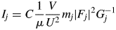
Theory of the DD method can be started from the intensity formula for powder diffraction (James, Reference James1967). For the jth reflection from a thick slab of powdered specimen in the Bragg–Brentano (BB) geometry, the integrated intensity, I j, can be calculated by
 $$I_j = C\displaystyle{1 \over \mu }\displaystyle{V \over {U^2}}m_j\vert {F_j} \vert ^2G_j^{{-}1} $$
where C represents the proportional constant including the wavelength of incident X-rays, the mass and charge of electron, the velocity of light in free space, the width of a receiving slit, and the goniometer radius, μ is the linear absorption coefficient, V is the irradiated volume of specimen, U is the unit-cell volume, m j is the multiplicity of reflection, F j is the structure factor, and  $G_j^{{-}1}$ represents the Lorentz-polarization factor and the geometrical factor. In the present case based on the BB geometry,
  $G_j^{{-}1}$ can be given by
  $G_j^{{-}1} = ( {1 + {\rm co}{\rm s}^22\theta_j} ) /( {2{\rm sin}\theta_j{\rm sin}2\theta_j} )$, when no monochromator on both incident- and diffracted-beam sides is assumed. By multiplying both terms of Eq. (1) by G j and summing up them, we obtain
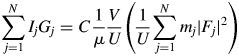 $$\mathop \sum \limits_{\,j = 1}^N I_jG_j = C\displaystyle{1 \over \mu }\displaystyle{V \over U}\left({\displaystyle{1 \over U}\mathop \sum \limits_{\,j = 1}^N m_j{\vert {F_j} \vert }^2} \right)$$
where N is the number of reflections in a wide 2θ-range defined by [2θ L, 2θ H]. In Eq. (2), 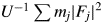 $U^{{-}1}\sum m_j\vert {F_j} \vert ^2$ is identical with a peak height at the origin of the Patterson function, P(0). We often approximate the integrated intensity of a reflection with its peak height. In the same manner but inversely in this case, the peak height, P(0), can be approximated by the integrated value of the peak, which can be given by
  $Z\sum n_i^2$, where Z is the number of chemical formula unit in the unit cell, n i is the number of electrons belonging to the ith atom in the chemical formula unit with the total number of atoms N A, and the summation is taken over N A atoms. Then, we obtain
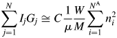
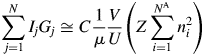 $$\mathop \sum \limits_{\,j = 1}^N I_jG_j\cong C\displaystyle{1 \over \mu }\displaystyle{V \over U}\left({Z\mathop \sum \limits_{i = 1}^{N^{\rm A}} n_i^2 } \right)$$
V/U in Eq. (3) represents the number of unit cell in the volume V, and it can equivalently be represented by W/ZM, where W is the weight of a specimen with the volume V and M is the chemical formula weight.Footnote 1 By replacing V/U with the W/ZM, we obtain
 $$\mathop \sum \limits_{\,j = 1}^N I_jG_j\cong C\displaystyle{1 \over \mu }\displaystyle{W \over M}\mathop \sum \limits_{i = 1}^{N^{\rm A}} n_i^2 $$
The V in Eq. (3) can also be represented by V = W(ZM/U)−1, where ZM/U is the density of the material, and it derives the same expression as Eq. (4). Equation (4) was first derived by using the approximation as described above: the relationship between the height and the integrated value of the peak at the origin of the Patterson function (Toraya, Reference Toraya2016). The expression, which is identical to that of Eq. (4), had also been derived in a more rigorous form, starting from the Debye equation, by integrating over the reciprocal space the scattered intensity from an assemblage of atoms at arbitrary positions [Eq. (15) in Toraya and Omote (Reference Toraya and Omote2019)]. Theoretical derivation by Toraya and Omote (Reference Toraya and Omote2019) for the random assemblage of atoms can also be applied to the ordered arrangement of atoms. Therefore, Eq. (4) is considered to be valid for both crystalline and noncrystalline materials.
In Eq. (4),  $\sum n_i^2$ represents the total scattered intensity from atoms in the chemical formula unit. Thus,
  $\sum n_i^2 /M$ represents the scattered intensity per unit weight. When the
  $\sum n_i^2 /M$ is multiplied by W, the product should give the total intensity from the specimen. Since W/M represents the number of chemical formula units in the specimen with the weight W, Eq. (4) can alternatively be interpreted as representing (the number of chemical formula unit) × (the scattered intensity from the chemical formula unit). Both interpretations give the same quantity of the total scattered intensity from the specimen, and they are consistent with the
  $\sum I_jG_j$ on the left-hand side of Eq. (4).
B. The intensity–composition formula
Let us consider a K-component mixture and introduce two parameters, S k and  $a_k^{{-}1}$, where the subscript k represents the kth component. The S k and
  $a_k^{{-}1}$ are given by
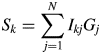 $$S_k = \mathop \sum \limits_{\,j = 1}^N I_{kj}G_j$$
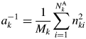 $$a_k^{{-}1} = \displaystyle{1 \over {M_k}}\mathop \sum \limits_{i = 1}^{N_k^{\rm A} } n_{ki}^2 $$
 S k represents the total sum of intensities corrected for the factor  $G_j^{{-}1}$, and it is an observable quantity.
  $a_k^{{-}1}$ represents the scattered intensity per unit weight, and its magnitude can be calculated only with the chemical composition data: the chemical formula weight and the numbers of electrons. Equation (6) does not include any crystallographic parameters like Z or U of component materials, and the input data required for calculating
  $a_k^{{-}1}$ are purely chemical. Equation (4) can be expressed by
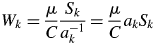 $$W_k = \displaystyle{\mu \over C}\displaystyle{{S_k} \over {a_k^{{-}1} }} = \displaystyle{\mu \over C}a_kS_k$$
In QPA, what we would like to find are the relative weight ratios of the individual components. Therefore, under the normalization condition, the weight fraction for the kth component, w k, can be calculated by
 $$w_k = \displaystyle{{W_k} \over W} = W_k\left({\mathop \sum \limits_{{k}^{\prime} = 1}^K W_{{k}^{\prime}}} \right)^{{-}1}$$
As long as intensities of individual components in a mixture, measured in a single scan, are compared, a single value of the linear absorption coefficient μ is shared with all components. Thus, μ and C in Eq. (7) are canceled out, when Eq. (7) is substituted into Eq. (8). Then, the w k is given by
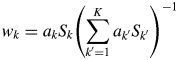 $$w_k = a_kS_k\left({\mathop \sum \limits_{{k}^{\prime} = 1}^K a_{{k}^{\prime}}S_{{k}^{\prime}}} \right)^{{-}1}$$
Equation (9) is called “the intensity–composition (IC) formula” as will be understood from two parameters S k and a k (Toraya, Reference Toraya2016).
C. Observed intensity datasets for individual components
As described above, the total sums of intensities (S k) for individual components are used as observed data in the IC formula. Various techniques of the powder pattern fitting can selectively be used for deriving {S k} for each sample. Fitting functions used in these techniques are currently classified into four types, A, B, C, and C2, and they are summarized in Table I (Toraya, Reference Toraya2019).
Table I. Fitting functions currently used for separating the observed pattern of a mixture into individual component patterns.
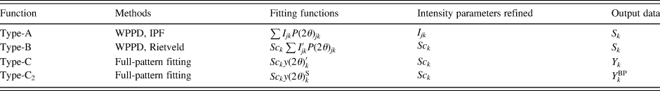
References for individual methods will be found in Section II.C.
A powder diffraction pattern of a mixture, y(2θ), is the superposition of individual component patterns, y(2θ)k, and it can be represented by
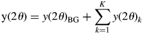 $${\rm y}( {2\theta } ) = y( {2\theta } ) _{{\rm BG}} + \mathop \sum \limits_{k = 1}^K y( {2\theta } ) _k$$
where y(2θ)BG is the background (BG) intensity, and some analytical functions, such as polynomials, can be used for modeling the BG. The type-A function is the fitting function widely used in the Pawley or Le Bail method for whole-powder-pattern decomposition (WPPD; Pawley, Reference Pawley1981; Le Bail et al., Reference Le Bail, Duroy and Fourquet1988). It can be expressed by  $y( {2\theta } ) _k = \mathop \sum \nolimits_j I_{kj}P( {2\theta } ) _{kj}$, where P(2θ)kj is the normalized profile function and I kj are adjustable. Individual profile fitting (IPF) techniques (Taupin, Reference Taupin1973; Parrish et al., Reference Parrish, Huang and Ayer1976) also belong to this group, and they can be used when reflections are sparsely distributed in a mixture pattern.
When strong parameter correlations of I kj are inevitable for heavily overlapping reflections, the type-B function can effectively be used. The type-B function uses a predetermined intensity parameter dataset  $\{ {I_{kj}^{\prime} } \}$. It can be defined by
 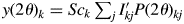 $y( {2\theta } ) _k = Sc_k\mathop \sum \nolimits_j I_{kj}^{\prime} P( {2\theta } ) _{kj}$, where Sc k is the scale parameter, and the Sc k is adjusted while
  $\{ {I_{kj}^{\prime} } \}$ are fixed at their original values in WPPF (Toraya and Tsusaka, Reference Toraya and Tsusaka1995). The intensity dataset
  $\{ {I_{kj}^{\prime} } \}$ can be obtained by decomposing a single-phase powder diffraction pattern of the kth component by using the WPPD methods or by calculation from the crystal structure parameters. When the type-B function is used, S k is given by
  $S_k = Sc_k\sum I_{kj}^{\prime} G_j$.
When the pattern decomposition nor the calculation from the crystal structure parameters is difficult for obtaining {I kj} or  $\{ {I_{kj}^{\prime} } \}$ as in the case of clay minerals with staking disorder, the type-C function can effectively be used. The type-C function uses a single-phase observed diffraction pattern after subtracting the BG just as in the full-pattern fitting method by Smith et al. (Reference Smith, Johnson, Scheible, Wims, Johnson and Ullmann1987). The profile intensity for the single-phase kth component material is represented by
 $$y( {2\theta } ) _k^{\rm S} = y( {2\theta } ) _{{\rm BG}\_k}^{\prime} + y( {2\theta } ) _k^{\prime} $$
where  $y( {2\theta } ) _{{\rm BG}\_k}^{\prime}$ is the BG intensity,
  $y( {2\theta } ) _k^{\prime}$ is the peak profile intensity, and a superscript S is used to denote “single phase”. The type-C function is given by
  $y( {2\theta } ) _k = Sc_ky( {2\theta } ) _k^{\prime}$, and the scale parameter Sc k is adjusted in WPPF. The total sum of intensities can be obtained by
 $$Y_k = Sc_k\;\int_{2\theta _{\rm L}}^{2\theta _{\rm H}} {y( {2\theta } ) _k^{\rm ^{\prime}} G( {2\theta } ) \;{\rm d}( {2\theta } ) } $$
where G(2θ) is the continuous form of G j. Since the definition of Y k by Eq. (12) is different from that of S k by Eq. (5), different symbols S k and Y k are used. However, S k and Y k can easily be verified to be equivalent for a pattern in the same 2θ-range [2θ L, 2θ H], and the Y k can equally be used in place of S k in Eq. (9) (Toraya, Reference Toraya2018).
When the BG subtraction is technically difficult as in the case of a halo pattern from an amorphous material, the type-C2 function can be used. The type-C2 function uses  $y( {2\theta } ) _k^{\rm S}$ for modeling a component pattern without subtracting the BG (Chipera and Bish, Reference Chipera and Bish2002), and it is simply defined by
  $y( {2\theta } ) _k^{{\rm BP}} = Sc_ky( {2\theta } ) _k^{\rm S} = Sc_k\;[ {y( {2\theta } )_{{\rm BG}\_k}^{\prime} + y( {2\theta } )_k^{\prime} } ]$, where superscript BP is used to mean BG + peak profile intensities. In this case,
  $Sc_ky( {2\theta } ) _{{\rm BG}\_k}^{\prime}$ works as a part of the BG model. The integration of
  $Sc_ky( {2\theta } ) _k^{\rm S} G( {2\theta } )$ in the range [2θ L, 2θ H] is given by
 $$ \eqalign{{Y_k^{\rm BP}} &= Sc_k\int_{2\theta _{\rm L}}^{2\theta _{\rm H}} {y( {2\theta } ) _{{\rm BG}\_k}^{\prime} G( {2\theta } ) \;{\rm d}( {2\theta } )}\cr & \hskip12pt + Sc_k \int_{2\theta _{\rm L}}^{2\theta _{\rm H}} {y( {2\theta } ) _k^{\prime} G( {2\theta } ) \;{\rm d}( {2\theta } ) }}$$
 By denoting the first term on the right-hand side of Eq. (13) by B k,  $Y_k^{{\rm BP}}$ can be expressed by
  $Y_k^{{\rm BP}} = B_k + Y_k$. Let us define a ratio of B k to Y k by R k = B k/Y k. Then, Y k can be obtained from
  $Y_k^{{\rm BP}}$ by
 $$Y_k = \displaystyle{{Y_k^{{\rm BP}} } \over {1 + R_k}}$$
 When the type-C2 function is assigned to modeling the kth component pattern, the  $Sc_ky( {2\theta } ) _k^{\rm S}$ is fitted and
  $Y_k^{{\rm BP}}$ is output. If we predetermine the magnitude of R k, the Y k can be derived from
  $Y_k^{{\rm BP}}$ with Eq. (14), and it can be used in Eq. (9) together with other S k and/or Y k. Two experimental techniques for determining values of R k are given in Toraya (Reference Toraya2019).
When the type-C2 function is assigned to all components in a mixture, the substitution of Eq. (14) into Eq. (9) gives
 $$w_k = \displaystyle{{a_kY_k^{{\rm BP}} } \over {1 + R_k}}\left({\mathop \sum \limits_{{k}^{\prime} = 1}^K \displaystyle{{a_{{k}^{\prime}}Y_{{k}^{\prime}}^{{\rm BP}} } \over {1 + R_{{k}^{\prime}}}}\;} \right)^{{-}1}$$
When the following approximation does hold
 $$R_1\cong R_2\cong R_3\cong \cdots \cong R_K$$
Equation (15) becomes
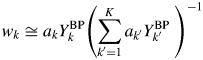 $$w_k\cong a_kY_k^{{\rm BP}} \left({\mathop \sum \limits_{{k}^{\prime} = 1}^K a_{{k}^{\prime}}Y_{{k}^{\prime}}^{{\rm BP}} \;} \right)^{{-}1}$$
Equation (17) has the same form as that of Eq. (9). In this case, the weight fraction w k can be derived by using the intensity datasets  $\{ {Y_k^{{\rm BP}} } \}$ of non-BG subtracted powder patterns, and the parameter R k is not required. For a mixture consisting of component materials with similar chemical compositions, the relation by Eq. (16) generally holds, and the type-C2 function gives very accurate results of quantification as will be shown later.
Important thing to be noted here is that four types of fitting functions given in Table I can arbitrarily be combined and be fitted simultaneously in WPPF for a mixture pattern, and an example will be shown later. The other thing is that the type-A function has the greatest degree of freedom in WPPF. The type-A function is the same as that used in Pawley refinement, and individual integrated intensities as well as unit-cell parameters, profile width, and shape parameters can be refined. When single-phase observed powder diffraction patterns are used as the type-C/C2 function, they should be measured under the same instrumental setup as that for measuring the target mixture patterns in order to reduce the model bias. In this sense, the type-C and type-C2 functions are less flexible compared with the type-A and B functions. They are, however, stable in the least-squares fitting and suitable for modeling complicated diffraction patterns in WPPF.
Regarding the effect of the preferred orientation on individual intensities, the DD method, utilizing the total sums of scattered/diffracted intensities is much less influenced than the single-peak intensity methods. The intensity data are, however, not corrected for the preferred orientation at present. The correction for the preferred orientation effect as well as micro-absorption effect are issues to be studied in the future.
D. Introduction of the normalized fitting function
Since Eq. (6) has been derived by summing/integrating all scattered/diffracted intensities in the reciprocal space, the definition range of 2θ for the corresponding total sums of observed intensities, defined by Eqs. (5) and (12), should also be extended to the maximum high-angle limit. In QPA using Eqs. (9) and (17), the relative intensity ratios of S 1: S 2: S 3: ⋅ ⋅ ⋅ :S K determine the weight fractions. When one component in a mixture has relatively strong peaks in the high-angle region, compared with the other components, the relative intensity ratios will be varied with whether these peaks are included or not in the range [2θ L, 2θ H]. The termination in summing/integrating observed intensities is, therefore, one of the possible sources of error in the derived weight fractions. In order to suppress the termination errors, the normalized fitting functions have been introduced (Toraya, Reference Toraya2020). In the case, for example, of type-C function, the normalized type-C function, denoted by  $y( 2\theta ) _k^{\rm N}$, can simply be defined by
 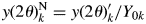 $y( 2\theta ) _k^{\rm N} = y( 2\theta ) _k^{\prime} /Y_{0k}$. Here, Y 0k is equivalent to Y k defined by Eq. (12). Then, the integration of
  $y( 2\theta ) _k^{\rm N}$ always gives unity, that is,
 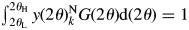 $\int_{2\theta _{\rm L}}^{2\theta _{\rm H}} {y( 2\theta ) _k^{\rm N} G( {2\theta } ) {\rm d}( {2\theta } ) = 1}$. In WPPF using the normalized type-C function,
  $Sc_k^{\rm N} \;y( 2\theta ) _k^{\rm N}$ is fitted, where
  $Sc_k^{\rm N}$ is the adjustable scale parameter for the normalized fitting function. Then, Y k, defined by Eq. (12), but for the normalized fitting function, is given by
  $Y_k = Sc_k^{\rm N}$.
The advantages of introducing the normalized fitting function are that the magnitude of refined scale parameter,  $Sc_k^{\rm N}$, is much less sensitive to the termination of the 2θ-range in WPPF. If we define the normalized fitting function by extending the [2θ L, 2θ H] to the high-angle limit such as
  $100^\circ$ or
  $120^\circ$ (for CuKα radiation), the 2θ-range in WPPF for target mixture patterns can be much shortened to, say,
  $60^\circ$. Therefore, we can save the time spent for intensity data collection without losing the accuracy in derived weight fractions (Toraya, Reference Toraya2020).
E. Calculation and some properties of a k
We can easily calculate a k values from the chemical composition data using a periodic table and a pocket calculator. Here, two examples are given. One is α-quartz with the chemical formula of SiO2. In this case, M k and  $\sum n_i^2$ are given by M k = 28.086 + 2 × 15.999 = 60.084 g mol−1 and
  $ \sum n_i^2 = $
  $ 14^2 + 2 \times 8^2 = 324$, respectively. Thus,
  $ a_k = M_k/\sum n_i^2 = $
  $ 0.18544$. The other example is a solid solution with the chemical formula, for example, Mg1.6Fe0.4SiO4. M k and
  $\sum n_i^2$ are given by M k = 1.6 × 24.312 + 0.4 × 55.847 + 28. 086 + 4 × 15.999 = 153.320 g mol−1 and
  $ \sum n_i^2 = 1.6 \times 12^2 + 0.4\, \times $
  $ 26^2 + 14^2 + 4 \times 8^2 = 952.8$. Thus, a k = 0.16092. For fractional atoms like Mgx, the
  $n_i^2$ should be counted as x × 122 but not as (x × 12)2. In the average structure, one crystallographic site is shared like MgxFe1−x. In real space, however, atoms at individual sites in a whole crystal scatter the
  $n_i^2$ of either 122 or 262 in an abundance ratio of x:1 − x.
To understand some properties of a k may be useful when the chemical composition data of target materials are more or less indefinite. In the first, the a k has the relationship represented by  $a_k^{{-}1} \approx A_k^{{\rm av}} /D$, where
  $A_k^{{\rm av}}$ is the average atomic weight of atoms in the chemical formula unit (
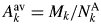 $\;A_k^{{\rm av}} = M_k/N_k^{\rm A}$), D is a ratio of atomic weight to atomic number, and D ≈ 2 (D = 2.006 in the case of Si) (Toraya, Reference Toraya2017, Reference Toraya2018). Table II gives the values of a k for two series of compounds (Toraya, Reference Toraya2017). In the case of hydrated magnesium silicate (HMS), the standard deviation of the average a k value is just 0.02%. These results mean that materials with similar chemical compositions give the a k's of almost the same magnitude. In the case of polymorph or polytypes, the a k's are equivalent, and we can derive individual weight fractions, w k, by the IC formula without using the a k. When four compounds of HMS in Table II are evenly weighed, mixed and quantified by using the average a k of 0.19022 instead of individual a k values, associated error in w k is just 0.02 wt% (Toraya, Reference Toraya2017).
Table II. A comparison of a k values for series of magnesium silicate hydrates and hydrocarbons with similar chemical compositions (Toraya, Reference Toraya2017).
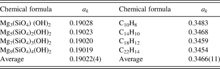
Values at the bottom line represent the averages of individual a k values and their standard deviations in parentheses.
As well known, chemicals compositions of natural products are complicated due to various degrees of cation substitution like Si ↔ Al, Mg ↔ Fe, as well as inclusions of trace elements, such as Li, Ti, Cr, Mn, Ni, Ca, Cs, and Ba. The chemical composition data of rock-forming minerals are reported from all over the world (Deer et al., Reference Deer, Howie and Zussman1971, Reference Deer, Howie and Zussman1976), and we can calculate the average of a k value, denoted by  $a_k^{{\rm av}}$, and its standard deviation,
  $\sigma ( {a_k^{{\rm av}} } )$, for each rock-forming mineral. As a practical example, a simulated QPA result is given for weathered granite, consisting of α-quart (SiO2), orthoclase (KSi3AlO8), albite (NaSi3AlO8), and biotite [K(Fe,Mg)3Si3AlO10(OH)2] in weight ratios of 48:37:11:4. Errors in w k, represented by Δw k, from assumed weight fractions were generated by varying a k by
  $a_k^{{\rm av}} \pm \sigma ( {a_k^{{\rm av}} } )$. The average values of |Δw k| were 0.33, 0.51, 0.10, and 0.16 wt% for respective minerals (a grand average of 0.27 wt%). These errors can also be estimated with the error estimation formula [Eq. (11) in Toraya (Reference Toraya2017)], and the magnitudes of estimated errors were 0.37, 0.48, 0.11, and 0.15 wt% (0.28 wt%), being in a good agreement with those in simulated QPA. These results mean that errors associated with possible variations in a k value will be in the order of <0.5 wt%, and they may be less for minerals from local mines with accumulated chemical analysis data.
When unknown material was found as one of the components in a mixture, its chemical composition can be estimated, as the first approximation, by the batch chemical composition of the sample. More accurate procedure for estimating a k and w k of the unknown material using the iterative procedure is described in Toraya (Reference Toraya2017).
III. EXPERIMENTAL AND DATA ANALYSIS
Intensity data collections can be conducted with an ordinary type powder diffractometer based on the Bragg–Brentano geometry. The G j in Eq. (5) or G(2θ) in Eq. (12) are needed to be modified accordingly, when the monochromator was used on the incident- or diffracted-beam sides, the other types of diffractometer were used, or the different scan-mode such as the asymmetric diffraction was employed. As was described above, the constant optical setting should be kept in measuring powder diffraction patterns of both target mixtures and single-phase components to be used as the type-C and/or the type-C2 functions. When the type-C/C2 functions were used, the shift of a whole pattern,  $y( {2\theta } ) _k^{\prime}$ or
  $y( {2\theta } ) _k^{\rm S}$, along the 2θ-axis, associated primarily with the shift in the height of a specimen surface, can be corrected by adjusting the parameter, Δ2θ k (Toraya, Reference Toraya2018) [δ 2θk is a different symbol (Toraya, Reference Toraya2019, Reference Toraya2020)]. Regarding the 2θ-range for scanning, [2θ L, 2θ H], the 2θ L should include the reflection at the lowest angle. The 2θ H should be extended to
  $100^\circ$ or
  $120^\circ$ (for the CuKα radiation), depending on the accuracy required. When the normalized fitting functions are used, the 2θ H for target mixtures can be lowered to
  $60^\circ$ or
  $70^\circ$.
A computer program, WPPF4.0 (version 4.00), written in Fortran 90 for the WPPD method (Toraya, Reference Toraya1986) has been used for data analysis, conducted by the author himself. Some software suites are commercially available. Although terms of type-A, B, C, and C2 functions were not used before, these four types of the fitting functions have already been equipped and used as they are classified in Table I. Therefore, existing computer programs for WPPD, Rietveld refinement, full-pattern fitting, etc. can also be used with a small modification or by adding a subprogram for calculating S k [Eq. (5)], Y k [Eq. (12)], and  $Y_k^{{\rm BP}}$ [Eq. (13)] together with a k values. The details of experimental and data analysis conditions for analyzed results given below will be found in respective references cited.
IV. RESULTS AND DISCUSSION
In the followings, five examples of applications of the DD method are presented.
A. Combined use of type-A, B, and C functions
A first example is the QPA of an artificial ternary mixture consisting of α-quartz (SiO2), albite (NaAlSi3O8), and kaolinite (Al2Si2O5(OH)4) in weight ratios of 5:4:1, which simulate weathered granites used as raw materials in the ceramics industry. Mixtures in weight ratios of 1:1:1 were also quantified (Toraya, Reference Toraya2018). α-quartz with a relatively small unit cell belongs to the trigonal symmetry, and it gives well-resolved peaks sparsely distributed in its diffraction pattern. On the other hand, albite belongs to the triclinic system, and it gives a lot of reflections heavily overlapping in a whole 2θ-range. As well known, kaolinite is a clay mineral, and it exhibits diffuse scattering caused by the stacking disorder. When these materials exist as a mixture, a straightforward application of the Pawley-based WPPD method is hard to decompose the mixture pattern into individual Bragg components with sufficient accuracy.
For separating the mixture pattern into individual component patterns, a strategy taken for this mixture sample was to assign the type-A, B, and C functions to α-quartz, albite, and kaolinite, respectively. Before applying these functions to the mixture pattern in WPPF, a single-phase diffraction pattern of albite was first decomposed to obtain an intensity dataset  $\{ {I_{kj}^{\prime} } \}$. In the case that the single-phase sample is not available, an alternative way may be to derive the
  $\{ {I_{kj}^{\prime} } \}$ by calculation using crystal structure parameters. Secondly, the BG of a single-phase diffraction pattern of kaolinite was subtracted to obtain
  $y( 2\theta ) _k^{\prime}$. In WPPF for the mixture pattern, I jk parameters of α-quartz were refined independently together with the scale parameters, Sc k, for albite and kaolinite patterns. The unit-cell parameters of α-quartz and albite were also refined together with the other parameters such as profile width and peak-shift correction.
For testing the reproducibility in this example, intensity measurements of the two mixture samples, as well as the three component materials, were repeated three times for each sample, repacked into a specimen holder prior to each scan. Before preparing the second mixture (1:1:1), a powder of kaolinite was additionally ground in an agate mortar in order to examine the influence of the degree of preferred orientation.
Table III gives the results of QPA. The root-mean-square error (RMSE) of Δw k was in the range 0.5–0.6 wt% for the 5:4:1 mixture, while it was in the range 1.6–1.9 wt% for the 1:1:1 mixture. The increase of the RMSE by ~1.2 wt% was ascribed to the different degrees of the preferred orientation of kaolinite particles between the two mixtures: kaolinite powder was additionally ground in preparing the second mixture, while the diffraction pattern of a kaolinite before additional grinding was used as the type-C function in the QPA of both mixtures. These results give a simple lesson that the diffraction pattern used for the type-C function should be close to that in the target mixture pattern.
Table III. Results of the QPA of two mixtures in weight ratios of 5:4:1 and 1:1:1.
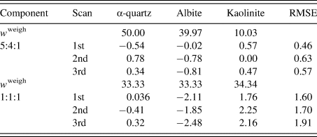
Numbers for each scan represent 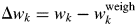 $\Delta w_k = w_k-w_k^{{\rm weigh}}$ (wt%), where
  $w_k^{{\rm weigh}}$ represents the weighed value of each component in sample preparation. The root-mean-square errors (RMSE) of Δw k for three components are given on the right-hand column (Toraya, Reference Toraya2018).
B. QPA using type-C2 function
1. QPA of  ${\rm \alpha }$- Al2O3 + ${\rm \gamma }$-Al2O3 binary mixtures


The second example is the use of the type-C2 function, applied to binary mixtures of α- and γ-Al2O3 in five different weight ratios (Table IV; Toraya, Reference Toraya2019). α-Al2O3 is chemically and thermally stable, and it is often used as a standard reference material, giving well-resolved peaks in a full 2θ-range. On the other hand, γ-Al2O3 has the structure of a defect cubic spinel type, and it gives broadened profiles and diffuse scattering as will be shown in Figure 1. Neither structure modeling from crystal structure parameters nor the pattern decomposition into Bragg components was difficult. Moreover, the diffuse scattering spread over the full 2θ-range made difficult to determine the accurate BG height. The type-C2 function is best suited for such a sample.

Figure 1. WPPF result for the diffraction pattern of α- and γ-Al2O3 mixture with a weight ratio of 5:95 (Toraya, Reference Toraya2019). The observed and calculated intensities are represented by plus symbols and solid lines, respectively. The plot at the bottom of the diagram represents the differences between the two intensities on the same scale.
Table IV.  $w_k^{{\rm weigh}}$ and Δw k (in wt%) for α- and γ-Al2O3 mixtures with five different weight ratios.
Data are given only for γ-Al2O3 since those for α-Al2O3 can be obtained by  $1-w_k^{{\rm weigh}}$ and −Δw k.
Both α- and γ-Al2O3 have the same chemical composition, and the relation R α ≅ R γ [Eq. (16)] was considered to hold. Then, single-phase powder diffraction patterns of α- and γ-Al2O3 were used as the type-C2 function. In WPPF to the mixture patterns, Sc k and δ 2θk for both components were refined together with the parameters in the BG function. Figure 1 shows a WPPF result for the mixture in weight ratio of 5:95. Table IV gives QPA results. An average value of Δw k for five mixtures was just 0.05 wt%. In the case of mixture in weight ratio of 95:5, it was hard to see a presence of γ-Al2O3 in the observed pattern. Nevertheless, γ-Al2O3 was accurately quantified. Simple adjustments of two single-phase diffraction patterns realize the accurate quantification of mixtures with complicated diffraction patterns.
2. QPA of amorphous component
QPA procedure used in the second example can directly be applied to mixture patterns containing an amorphous component. The third example is binary mixtures of α-quartz (SiO2) and glass-SiO2 in four different weight ratios (Table V). As in the previous example, the diffraction pattern of single-phase α-quartz and the halo pattern of glass-SiO2 were separately measured, and both patterns were used as the type-C2 function without subtracting their BG. Figure 2 shows a WPPF result for a mixture in weight ratio of 2:8. When the type-C function, instead of the type-C2, was assigned to the glass-SiO2 in WPPF for the same mixtures, the scale parameter for the glass halo pattern was interacted with the parameters in the BG function, and errors were increased with decreasing the content of glass-SiO2 (Toraya and Omote, Reference Toraya and Omote2019). The type-C2 function can avoid this parameter interaction, and it contributed to obtain accurate QPA results as indicated in Table V. Δw k values on the two lines in Table V were obtained with and without using the BG function for modeling the BG. These results indicate that the sum of the BG intensities from both component patterns, represented by  $Sc_ky( {2\theta } ) _{{\rm BG}\_{\rm \alpha }{\hbox -}{\rm quartz}}^{\prime} + Sc_ky( {2\theta } ) _{{\rm BG}\_{\rm glass}{\hbox -}{\rm SiO}_2}^{\prime}$, works for modeling the BG of the observed mixture patterns.
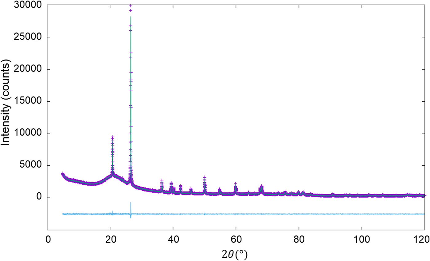
Figure 2. WPPF result for the diffraction pattern of α-quartz (SiO2) and glass-SiO2 mixture in a weight ratio of 2:8 (Toraya, Reference Toraya2019). Data are plotted as in Figure 1.
Table V.  $w_k^{{\rm weigh}}$ and Δw k (in wt%) for α-quartz (SiO2) and glass-SiO2 mixtures with four different weight ratios.
Data are given only for glass components. |Δw k|av represents the average of four |Δw k| (Toraya, Reference Toraya2019). Δw k values on the first line were obtained without the correction by the BG function and those on the second line by adjusting 8 BG parameters.
3. QPA of starch
The fourth example is the QPA of binary mixtures consisting of potato starch [(C6H10O5)n] and corn starch (C27H48O20) artificially mixed in five different weight ratios (Table VI). Figure 3 shows the powder diffraction patterns of the mixtures together with those of single-phase potato and corn starches. Although the two single-phase diffraction patterns indicate clear differences at some strong peaks while they are very similar to each other in other angular regions, and the mixture patterns gradually change between the two ends. The QPA of such materials has been very difficult because the RIR values are not available for these materials in the database. Structure-based Rietveld QPA could also be infeasible. In the present case, the single-phase diffraction patterns of potato and corn starches were used as the type-C2 functions, and they were fitted in WPPF to the mixture patterns. The results of QPA are given in Table VI, giving errors of just 1.2 wt% in their average.
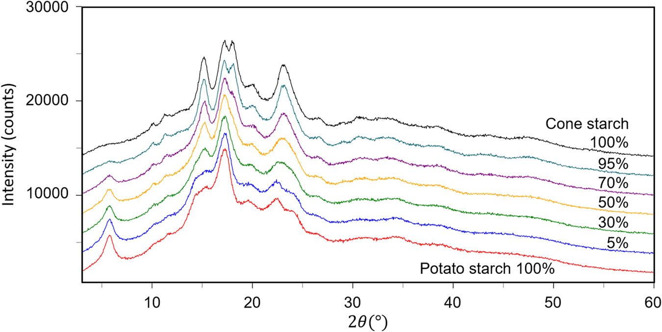
Figure 3. Powder diffraction patterns of potato starch, corn starch, and their mixtures in weight ratios indicated in the diagram.
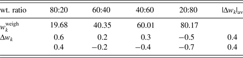
Table VI.  $w_k^{{\rm weigh}}$ and Δw k (in wt%) for corn starch in corn–potato starch mixtures.
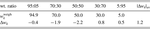
Data are given only for corn starch. |Δw k|av represents the average of five |Δw k|.
4. QPA of crystalline phase present in a very small amount in a mixture
The QPA of crystalline phases present in a very small amount, say <0.5 wt%, in mixtures is a very important issue in quality control of industrial products as well as in the research and development. The last example is the QPA of mixtures of (a) α-SiO2 + α-Al2O3 (SA) and (b) glass-SiO2 + α-SiO2 (GS) in five different weight ratios (Table VII), where the second components represent minor phases (Toraya, Reference Toraya2020). As shown in Figure 4, the presence of crystalline phases as minor components can be discerned as tiny peaks in both mixtures.
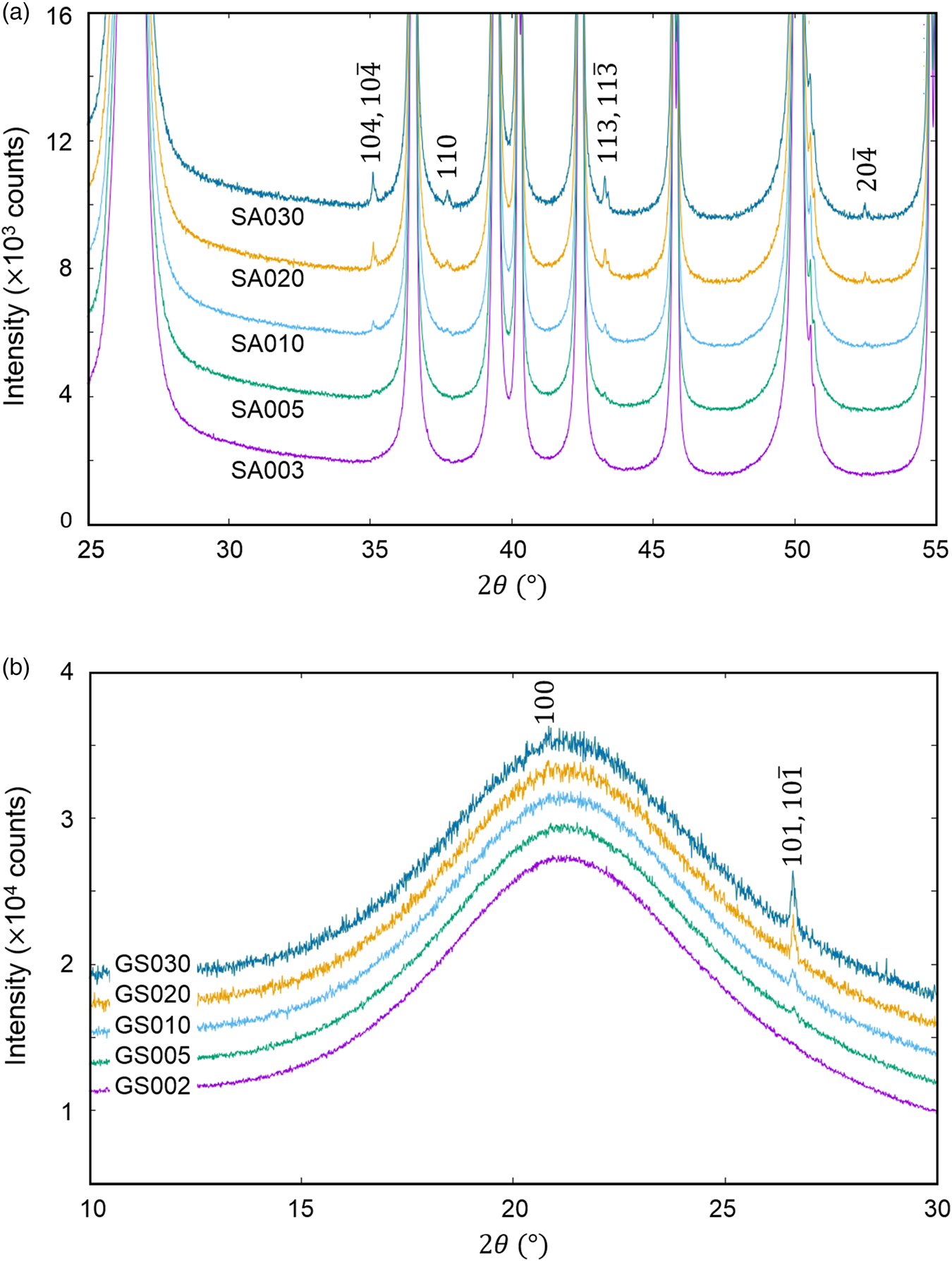
Figure 4. Observed powder diffraction patterns (parts) of (a) mixtures SA and (b) GS. Individual patterns are vertically shifted from each other at equal intervals of 2000 counts. Indices in the diagrams represent reflections from (a) α-Al2O3 and (b) α-SiO2 (Toraya, Reference Toraya2020).
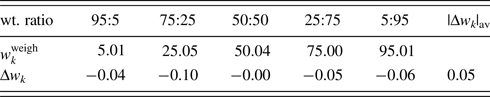
Table VII.  $w_k^{{\rm weigh}}$ and |Δw k|av (in wt%) for two series of mixtures SA and GS.
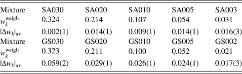
Data are given only for minor phases, A and S. Numbers in parentheses for |Δw k|av represent the standard deviations for respective averages (Toraya, Reference Toraya2020).
In WPPF, the normalized type-C2 function was assigned to all component in SA and GS mixtures. In Table VII, |Δw k|av represents the average of five |Δw k|, individual values of which were results of WPPF in the range of  $2\theta _{\rm H}$ = 60°, 70°, 80°, 90°, and 100° (
 $2\theta _{\rm L} = 15^\circ$). As clearly be shown in the very small standard deviations of 0.001–0.003 wt% for the |Δw k|av, the scale parameters (
 $Sc_k^{\rm N}$) were almost unvaried against the change of 2θ-range in WPPF. In this case, QPA could be conducted in the accuracy of 0.01–0.03 wt% for the mixtures containing component materials in wt% of 0.02–0.4.
V. SUMMARY
Theoretical background of the DD method and examples of applications have been described in this report. Some descriptions with many equations would give an impression that the DD method is a complicated technique. The DD method itself is, however, very simple, and it can simply be expressed by the IC formula [Eq. (9)]. It is based on a principle that the weight proportion for a component material can be given by dividing the total sum of scattered/diffracted intensities by the scattered intensity per unit weight represented by the symbol,  $a_k^{{-}1}$. Moreover, the magnitude of the
  $a_k^{{-}1}$ can be calculated only with the chemical composition data of that component material. Therefore, as indicated with several examples of applications given in this report, the DD method can be applied to the variety of materials from highly crystalline state to noncrystalline state just with the IC formula. Only a technical problem is how to separate the powder diffraction pattern of a target mixture into individual component patterns.
Various existing techniques can be used for tackling the problem. In the present report, four types of the fitting functions for WPPF are described. What we need as final outputs as the observed data in powder data analysis are  $ S_k, \;\;Y_k,$
  ${\rm and}/{\rm or\;}Y_k^{{\rm BP}}$. For this purpose, for example, even intensity datasets in d-I data in the PDF or instead the corresponding observed peak intensities can be used for calculating S k by Eq. (5). The relative weight ratios can be output immediately after the phase identification if a rough estimate of relative weight ratios suffices. As another way, currently used computer programs can also be used with small modification. For example, if we add the type-C and the type-C2 functions for modeling the amorphous components to a computer program for Rietveld refinement, the weight fractions can directly be output not only for crystalline phases but also for noncrystalline phase without doping the standard reference material nor conducting preliminary experiment. Individual techniques for separating the mixture patterns look sometimes complicated. In other words, however, there are various ways to solve a simple problem of just obtaining
  $ S_k, \;\;Y_k,$
  ${\rm and}/{\rm or\;}Y_k^{{\rm BP}}$.
ACKNOWLEDGEMENTS
The author thanks Yukiko Namatame of Application Laboratory, Rigaku Corporation (RC). All intensity datasets used in a series of studies on the DD method were collected by her. QPA results for mixtures of starches were also provided by her.


 Open access