Photogrammetry for Free Surface Flow Velocity Measurement: From Laboratory to Field Measurements

Abstract

This study describes a multi-camera photogrammetric approach to measure the 3D velocity of free surface flow. The properties of the camera system and particle tracking velocimetry (PTV) algorithm were first investigated in a measurement of a laboratory open channel flow to prepare for field measurements. The in situ camera calibration methods corresponding to the two measurement situations were applied to mitigate the instability of the camera mechanism and camera geometry. There are two photogrammetry-based PTV algorithms presented in this study regarding different types of surface particles employed on the water flow. While the first algorithm uses the particle tracking method applied for individual particles, the second algorithm is based on correlation-based particle clustering tracking applied for clusters of small size particles. In the laboratory, reference data are provided by particle image velocimetry (PIV) and laser Doppler velocimetry (LDV). The differences in velocities measured by photogrammetry and PIV, photogrammetry and LDV are 0.1% and 3.6%, respectively. At a natural river, the change of discharges between two measurement times is found to be 15%, and the corresponding value reported regarding mass flow through a nearby hydropower plant is 20%. The outcomes reveal that the method can provide a reliable estimation of 3D surface velocity with sufficient accuracy.

1. Introduction

The ability to measure flows in the vicinity of hydropower plants has undeniably wide applications. Especially in cases of plant changes, optimization of water utilization, or changing operating conditions, flow-related parameters often need to be taken into account. Among those parameters, flow velocity distribution over a large area undoubtedly contributes to the understanding of natural phenomena and leads to a better basis for decision making. The measurement task usually requires extensive investigative work due to complicated geometry, large volumes, transient effects. The use of the image analysis technique makes it possible to capture the surface-water velocity distribution over a large area outdoors without interference of normal plant operation.

For river flow, traditional ways to measure flow velocity usually require contacting waterbodies such as acoustic Doppler current profile [1], acoustic Doppler velocimetry, current meters [2], or velocity propellers. These velocity measurement methods are time-consuming, and the data obtained usually offer poor spatial coverage (i.e., point measurement). Moreover, for safety reasons, there are usually flow limitations which, for a regulated river, might interfere with hydropower generation. Among various new generations of measurement instruments, optical systems and image analyses have contributed to advance hydrological observations in several fields, for instance, precipitation and streamflow [3,4]. Furthermore, with the development of affordable high quality unmanned aerial vehicle (UAV) technology in combination with increased payload, these techniques open a potential application for flow measurement [5,6] and help to overcome the restrictions of traditional methods.

For free surface velocity monitoring based on image analysis, there are various algorithms that can be divided into three main approaches. The first approach was originally introduced in [7], so-called large-scale particle image velocimetry (LSPIV), which is an extension of PIV to provide velocity fields of large flow areas. The LSPIV image processing algorithm is similar to traditional PIV since the water surface is divided into sub-regions represented by groups of particles. These sub-regions function as tracers that can be tracked in image sequences using correlation to match flow patterns between successive images [7]. The approach has been widely applied for river flow measurement in previous studies [8,9,10]. Moreover, Fujita et al. introduced an image analysis technique called space-time image velocimetry (STIV) [11]. The method is capable of measuring the orientation angle of the pattern generated from the brightness distribution of the river surface along the time axis for monitoring streamwise velocity distributions.

The second approach is based on the optical flow algorithm. Perks et al. used the Kanade–Lucas–Tomasi (KLT) algorithm to track features present on the water surface that are related to the free-surface velocity to measure large floods [12]. A new motion estimation technique based on traditional optical flow was presented in [13] to monitor river velocity. Tauro et al. introduced a novel optical flow scheme, so-called optical tracking velocimetry (OTV) that combined feature detection, feature tracking and trajectory-based filtering to estimate the surface velocity field of natural streams [3].

Finally, particle tracking velocimetry (PTV), which consists of particle identification and tracking [14], is a promising image-based approach for remote streamflow measurements in natural environments [3]. In general, images are processed to enhance the appearance of particles in the field of view, and the locations of the particles’ centroids are recovered. The centroids of the detected particles are identified in subsequent images to reconstruct the particle trajectory [3]. Among diverse developed algorithms for PTV analysis, cross-correlation has emerged as the most commonly used technique implemented for particle detection and tracking. For instance, Lloyd et al. developed a correlation-coefficient based PTV to obtain surface velocity fields in unsteady flows over relatively wide areas [14]. Additionally, an integrated cross-correlation and relaxation algorithm for PTV was proposed in [15] to provide a flexible methodology that enables image analysis for different seeding and flow conditions. Dal Sasso et al. explored an optimal experimental setup for surface velocity measurement using cross-correlation based PTV [16]. More recently, Eltner et al. applied both terrestrial and UAV imagery for surface flow velocity and discharge estimation [17].

Among the alternative approaches applied for water surface flow measurement, PTV offers several advantages. PTV enables detecting and reconstructing the trajectories as well as velocity vectors of individual particles or features conveyed on the flow. Moreover, tracking individual particles in PTV does not suffer from spatial averaging, and bias errors can, therefore, be reduced [18]. However, the field condition imposes several challenges; for instance, PTV is dependent on the tracers or structures transiting on the water surface. Having a sufficient number and uniquely recognizing such surface structures on natural streamflow without the need of excessive seeding is a challenging problem. Furthermore, seeding a large field of view constitutes a major problem both from practical and environmental perspectives. Alternatively, LSPIV may be utilized without deploying tracers in the flow in such conditions. The relative performance of LSPIV and PTV for surface velocity measurements in natural streams was investigated in [19].

One thing in common from the above-mentioned literature reviews is the utilization of a single camera in the measurement, resulting in two-component vector fields representing longitudinal velocity and transverse velocity components, respectively. This approach assumes the water surface to be a plane and suggests avoiding camera setups with large tilting angles [20]. However, during high flows or in nonuniform depth flows, the water surface would present strong undulation. In those cases, the third velocity component in the vertical direction would give more information about the shape of the flow. In addition, most approaches orthorectify the images prior to tracking to allow for a correct scaling of the image tracks, and such a process may lead to interpolation errors [17].

Regarding the application of photogrammetry in 3D surface flow measurement, multiple synchronized digital cameras were used in combination with a commercial close-range photogrammetric package PhotoModeler for data processing to achieve 3D water surface and surface velocity of a water flume and a natural river [21]. However, their surface velocity measurement required lots of manual intervention in the data processing. Hoshino and Yasuda developed a flume experiment-based 3D measurement to measure water and bed surface during the formation of sand waves using photogrammetry [22]. In their study, the water surface was estimated by calculating the intersection points of laser light and camera rays. More recently, Li et al. developed a stereo imaging based LSPIV system to measure surface velocity and reconstruct the water surface distribution of a mountainous stream [23]. The study revealed that the velocity measurement and discharge estimation could be improved with 3D water surface distribution.

The present study aims to investigate the applicability of using multiple cameras in one photogrammetry-based PTV system to estimate surface velocity for both laboratory water flume and natural river flow. Two camera calibration procedures for the two circumstances mentioned above are proposed. The measurements apply different seeding tracers that require two different methods used to detect and track surface particles, in conjunction with filtering techniques used in this work. The estimated surface velocity of the laboratory water flume is compared to that measured by traditional measurements (i.e., PIV and LDV). For the evaluation of the outdoor measurement results, the change in determined flow rate through the nearby hydropower plant is used to roughly compare the change in measured surface velocity. The experimental setups utilized for the laboratory and the river flow measurements, respectively, are introduced in Section 2. The camera calibration methods and accuracy estimation are presented in detail in Section 3. Section 4 presents the data analysis performed, while the results are presented and discussed in Section 5. Finally, the paper ends with some conclusions.

2. Measurement Sites and Measurement Setup

The utilization of multiple cameras in one photogrammetric system enables to fully achieve the 3D shape and velocity components of surface flow. It, however, raises some challenges in measurement setup as well as in data analysis. Luhmann showed that an appropriate design, setup, and operation of a photogrammetric system imposes a complex task [24]. In this study, the precision of the measurement is not only a question of technical issues (i.e., camera stability, synchronization, acquisition and data transfer speed, and representation of surface features) but also a requirement of image processing and 3D reconstruction methods (i.e., feature tracking, multiple-image matching approach, and method for determination of 3D coordinates). Therefore, it is important to investigate the properties of the photogrammetric system and PTV algorithm in surface velocity estimation to prepare for the field measurements. For this purpose, the surface velocity measurement of a water flume in the laboratory is utilized to evaluate the applicability of a photogrammetry-based PTV system.

2.1. Measurement in Laboratory Water Flume

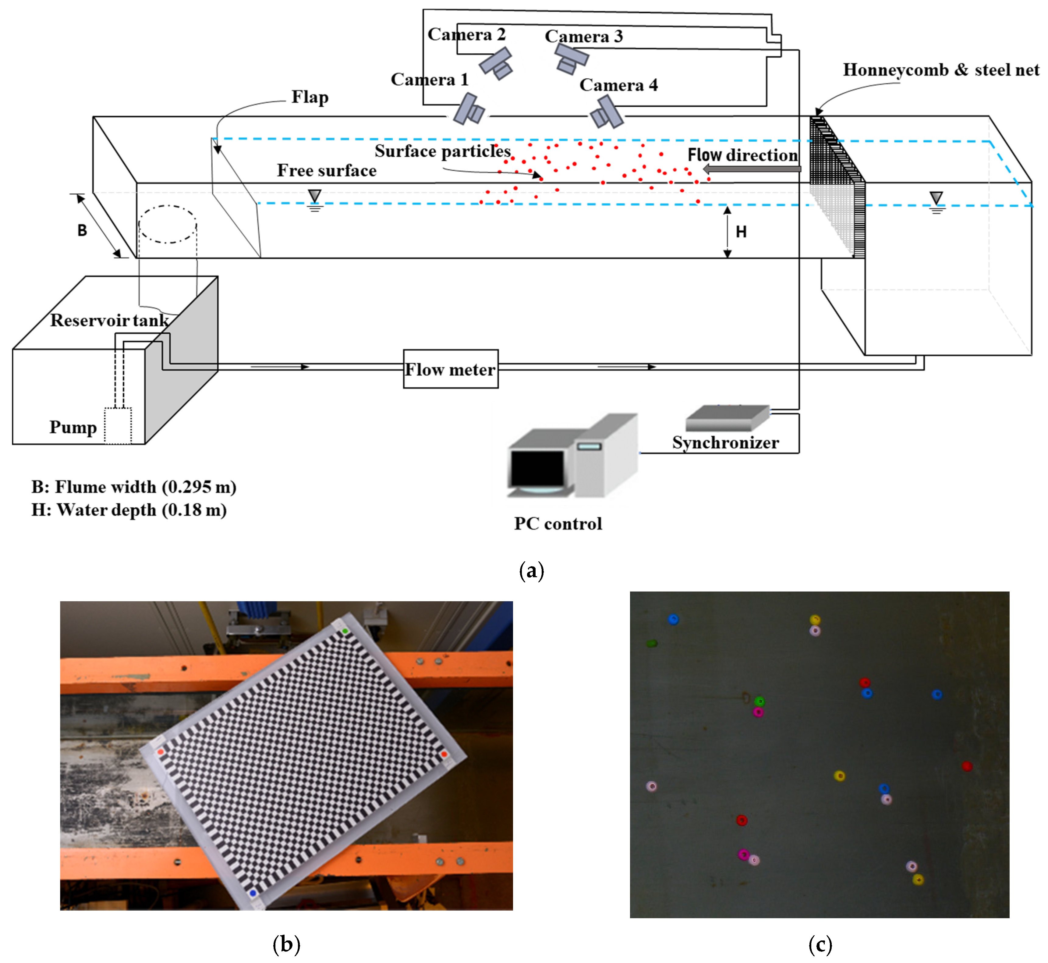
The surface velocity measurement in the laboratory was carried out using a photogrammetric system consisting of four cameras. A sketch of the experimental setup is presented in Figure 1a. Figure 1b shows a checkerboard pattern used for camera calibration. The flume has a dimension of 7.5 m × 0.295 m × 0.310 m in length, width, and height, respectively. There is a steel net and honeycomb at the inlet of the channel to provide a uniform inflow. The honeycomb has a thickness of 75 mm and the diameter of its holes is 7.6 mm. The thickness of the steel net is 0.08 mm, and it consists of 2.5 mm × 2.5 mm square holes [25] (Figure 1a). The observed flow area was 0.7 m × 0.3 m. The water was typically clear and transparent. In such a condition, the images taken of the water flow showed only the bottom of the flume and reflections from the light source. To provide structure on the water surface, 4 mm diameter spherically shaped wooden beads were used, as shown in Figure 1c. Additionally, because the water flow moved predominantly in one direction along the channel, interactions between the particles were assumed to contribute negligibly to the surface velocity outcomes. In order to validate this surface velocity measurement, the experiment was set up to carry out in the same condition with previously performed PIV and LDV measurements [25]. The flow rate was 4.17 L/s, the water depth was 180 mm, and the Froude number was 0.08. The flow can be considered subcritical. The PIV and LDV measurements captured the streamwise mean velocity profile along the centerline of the flume. The nearest locations from the water surface where the velocities can be measure by PIV and LDV were at 30 mm under the water surface. The velocities at these locations will be used to compare to surface velocity measured by the photogrammetry (see Section 5.1).

The laboratory photogrammetric system consisting of four cameras was mounted onto a testing frame to ensure a high stability system. The cameras with fixed positions and orientations were installed relative to each other in an array with an overlapping field of view of 0.8 m × 0.8 m and aimed toward the measurement volume, as shown in Figure 1a. All cameras were synchronized and triggered using an Arduino microcontroller and controlled by software on a computer. Acquisition of synchronized images was performed at an image resolution of 7360 × 4912 pixels using Nikon D800 cameras (Nikon Imaging Japan Inc., Tokyo, Japan), equipped with 35 mm lenses. The frame rate of 3.1 frames per second is roughly calculated in laboratory condition. The actual time intervals between consecutive captures are accurately recorded by control software.

2.2. Measurement in River Flow

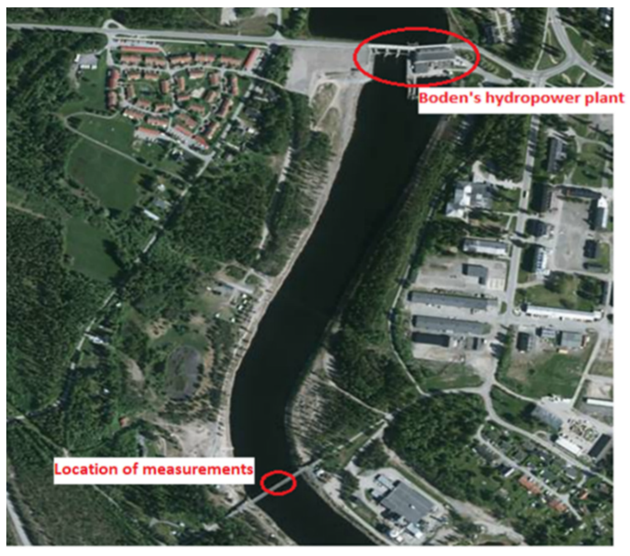
The measurement of the river flow velocity faces several important issues concerning the possibility of mounting several cameras with a clear view of the water surface. In addition, the stability of the camera system needs to be secured, as the precision of the measurement relies on the camera positions and orientations during image acquisition (see Section 3 for camera setup). The measurement site must be convenient for particle seeding in case there is no natural surface pattern or visible tracer in the flow. The location of the field measurement campaigns was a reach of Lule river in Boden, Sweden (Figure 2), about 0.8 km downstream from Boden hydropower plant. The measurement procedure took place from a bridge crossing the river reach that allowed a convenient setting for both camera setup and particle seeding. The field measurements were carried out in daylight conditions, and the river flow was clean. There was no suitable texture of the water surface itself to enable a reliable surface particle or surface pattern for image-based data. Instead, the usefulness of crushed leaf, oranges, and puffed corn was evaluated as suitable particles for surface seeding. In clear water conditions, these tracers show a good level of contrast with respect to the background. The measurements were performed successively in two days at the same river reach.

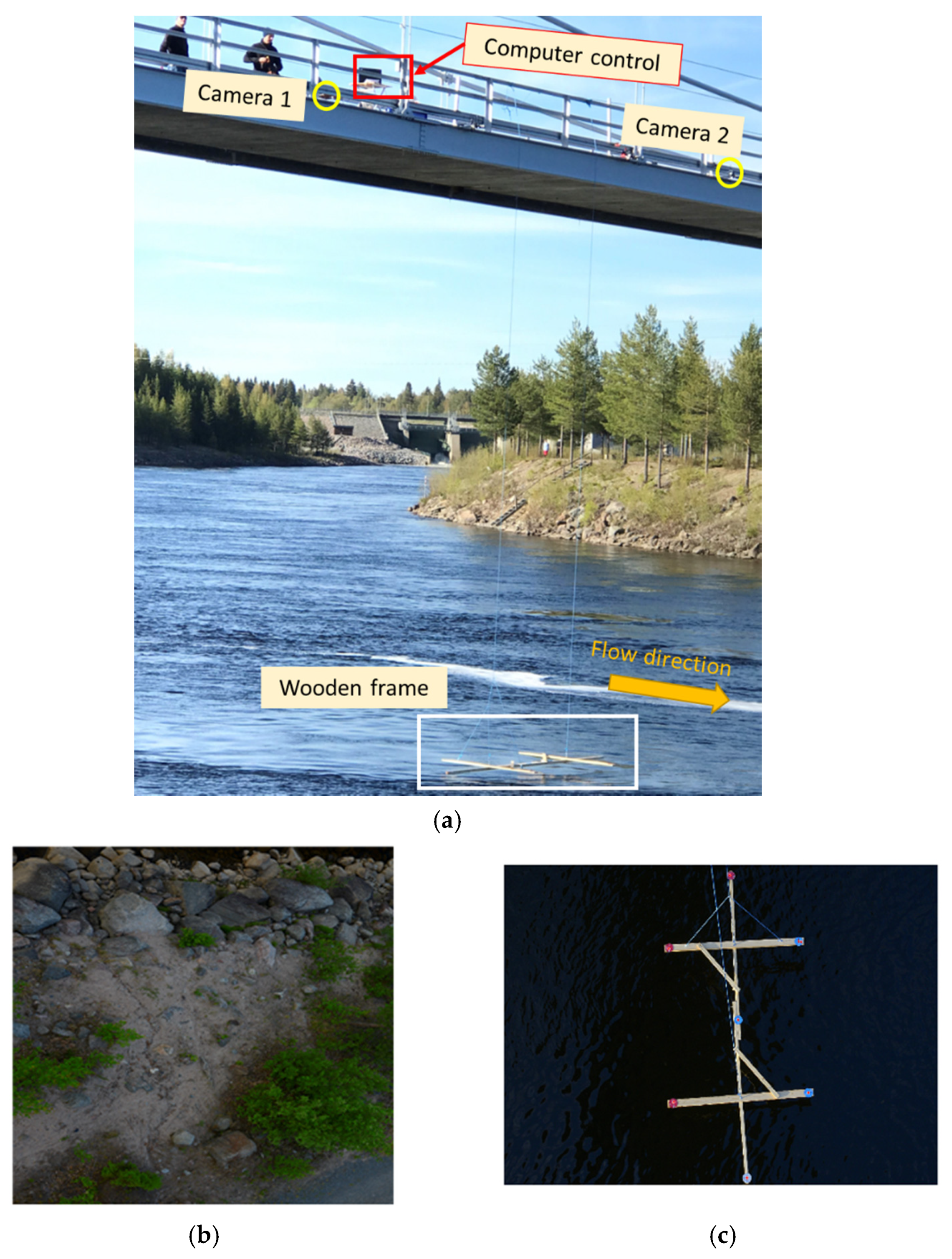
The same cameras and synchronization were used for the river flow measurements. However, for practical reasons, only two of the cameras were used, and they were mounted firmly on the bridge railing 7 m apart facing downwards into the river 12 m below, as shown in Figure 3a. The setup delivered a field of view of 11.0 m × 8.2 m. One pixel corresponds roughly to 1.5 mm × 1.7 mm.

3. Camera Calibration and Accuracy Estimation

In a photogrammetric system, the camera calibration procedure plays an essential role since it is directly related to measurement accuracy [24]. In order to enable high precision measurement, in situ calibration methods were used to mitigate the instability of the camera mechanism and camera geometry.

3.1. Camera Calibration for Laboratory Measurement

For the measurement in the laboratory, the checkerboard pattern (Figure 1b) was used. The checkerboard pattern was 49 cm × 35 cm and was placed in 40 arbitrary positions and orientations in the measurement volume. The intrinsic and extrinsic camera parameters were estimated from the detected calibration pattern, see [26,27]. The camera calibration gives a high precision pattern identification with a mean extrinsic reprojection error below 0.70 pixels for all cameras. The evaluation of the camera calibration uses additional 10 captures of the calibration pattern. These captures are separate from the images used in the calibration process. The camera calibration accuracy is calculated based on the error estimation in the measured distances between adjacent corners of the calibration pattern squares compared to the true square sizes (8.0645 mm). The accuracy of the synchronization and triggering of the cameras is very high. Therefore, the error in time is assumed to be negligible. The average of differences in distances gives a systematic error of 0.002 mm, while the standard deviation of differences in distances gives a precision of 0.023 mm, which corresponds to 0.03% on the measured velocities.

3.2. Camera Calibration for Field Measurements

Outdoor measurements were conducted with the cameras installed at the bridge across the river, see Figure 3a. The camera calibration was executed on-site based on multiple images recorded at the test field. The intrinsic and extrinsic camera calibrations were performed separately. Thereby, the intrinsic parameters were analyzed from sequential image captures, each camera individually, of a natural rock surface on the riverbank (Figure 3b) with a distance similar to that between the cameras and the water surface used in the measurements. For this purpose, the commercial photogrammetric software Agisoft Metashape 1.5.0 was used. The extrinsic calibration was performed by employing a wooden frame with fixed control points (Figure 3c) in the intersection field of view of the two cameras. The intrinsic camera parameters obtained from Agisoft Metashape and coordinates of control points were subsequently used to determine the positions and orientations of the cameras installed at the bridge. There are a total of seven image captures on day 1, and seven image captures on day 2, capturing the wooden frame at arbitrary positions and orientations in the measurement volume. For each measurement, there is only one capture used for extrinsic camera calibration. The remaining captures are used to estimate the accuracy of the camera calibration. The camera calibration was repeated at the beginning of each measurement day. Using the same method applied to calculate the accuracy of camera calibration in the laboratory, the accuracies of the camera system in the field measurements are estimated by utilizing the reference points on the wooden frame. The averages of distance errors are found to be 0.31 mm (day 1) and 0.48 mm (day 2). In addition, the standard deviations of differences in distances give a precision of 18 mm and 26 mm for day 1 and day 2, which correspond to 1.6% and 2% on the measured velocities for day 1 and day 2.

4. Image-Based Data Analysis

The procedure of data analysis presented in this paper relies on the basic principle of 3D-PTV. Therein, the motion of the surface tracers in the flow is recorded by the synchronized camera system resulting in a set of image coordinates of particles that are detected in all frames of each set, and 3D coordinates are derived from the camera calibration parameters. The 3D movements, and hence velocity components, are calculated from the relative movements on each camera detector between two consecutive images that are subsequently translated into a 3D velocity field using backprojection. This section presents in detail the techniques used in data analysis to determine the surface velocity.

Regarding surface particles used in this study, it should be noted that there are different types of tracers seeded into the flow corresponding to two practical situations. Therein, the laboratory measurement used the spherically shaped wooden beads, seen in Figure 1c, while the river flow measurement employed oranges, puffed corn, and crushed leaf for flow seeding. The difference in shape, size and density of the seeding particles lead to two different methods for particle detection. Thereby, the method utilized to detect the wooden particles in the laboratory measurement is applied for the images of the river flow with oranges. The small size high density puffed corn and crushed leaf pattern were instead analyzed using correlation-based particle clustering tracking. In the latter case, therefore a sub-region representing a group of particles is used for identification.

4.1. Particle Tracking

In this study, the spherically shaped particles are detected by using the Maximally Stable Extremal Regions (MSER) algorithm [28,29], resulting in the detected features in terms of regions. The function automatically filters out inappropriate features or regions to keep only reliable particles for tracking. Even though the function works robustly, the number of detected regions representing one particle could be greater than one, which leads to overlapping regions. This causes confusion in determining homologous particles between the cameras since representative points are close relative to each other. In order to eliminate that ambiguity, a clustering method is used to group the nearest regions into one via given threshold values of distance between the presentative center points.

Each image point corresponds to a ray from the measurement volume to the sensor of the camera. Particles are identified using analysis of ray bundles of detected features for all cameras in the network. The spatial 3D coordinates of particles are determined using Delaunay tessellation [30] and nearest neighbor methods [31] of the best intersection points of different rays in the ray bundles. Since we only consider surface movements, detected particles far away from the water surface are considered as misdetected and are therefore excluded from further analysis. Initially, a plane is roughly fitted to the surface points giving an estimate of the surface geometry. Detected surface points far away from this plane are excluded.

Assuming the flow motion between two consecutive images to be small, the transformation of the particle pattern on the surface is almost a rigid body transformation. The movements of particles are determined using a robust iterative closest point algorithm [32], where a rigid body transformation is estimated. Afterward, the nearest neighbor function is used to identify particle movements and to estimate a threshold value for an outlier filter. If a particle is estimated to have a movement larger than the threshold, it is considered as erroneous and is eliminated from the velocity estimation. The maximum track length is estimated from an average value of the movements of all detected particles obtained from previous steps. Finally, detected movement between two consecutive image captures divided by the elapsed time determines the velocity of each particle.

In summary, there are three criteria presented in this paper to increase the reliability of surface flow velocity estimation, including (i) clustering detected particles from overlapping, (ii) range of water surface and (iii) deviation from the average movement of the particles. The particle detection and tracking was performed for 20 and 14 images for the laboratory and the field measurements, respectively. New particles could be detected in every frame, and corresponding particles could be re-detected and tracked in the next frame as long as all criteria are fulfilled. Some results are shown in Figure 4, Figure 5 and Figure 6, respectively.

4.2. Correlation-Based Particle Clustering Tracking

This section describes the particle clustering tracking applied for image data of crushed leaves and puffed corn of the field measurements. Since the floating tracer introduced onto the flow partly covers the water surface in inhomogeneous concentration, the sub-regions with high-density surface patterns are manually chosen for tracking. As the camera system is calibrated, it is possible to determine the spatial 3D position and the orientation of the surface normal of the sub-region chosen. The center of each sub-region is denoted surface point. The correlation is based on projecting the points sub-regions onto the images of each camera in the network to get corresponding points image regions. Due to the slight movement of the surface points between two consecutive captures, detection of corresponding movements in the camera images is obtained using image correlation by searching in the subsequent image in a region near the projected initial surface point in the reference image. A number of trials perform the correlation procedure, where the trial having the highest correlation gives the detected movement in that camera. The spatial movement of the surface point is obtained from all cameras in the network between the reference capture and the subsequent one. Some results from this procedure is shown in Figure 6.

5. Results and Discussions

5.1. Surface Velocity of the Laboratory Water Flume

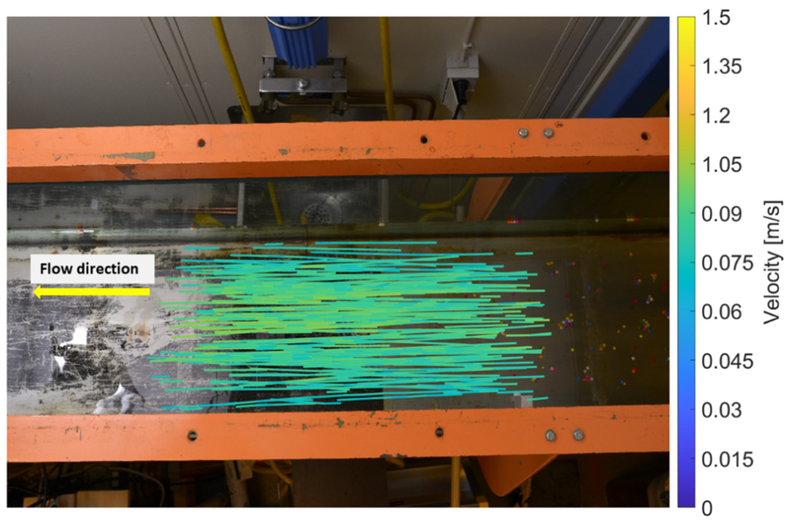
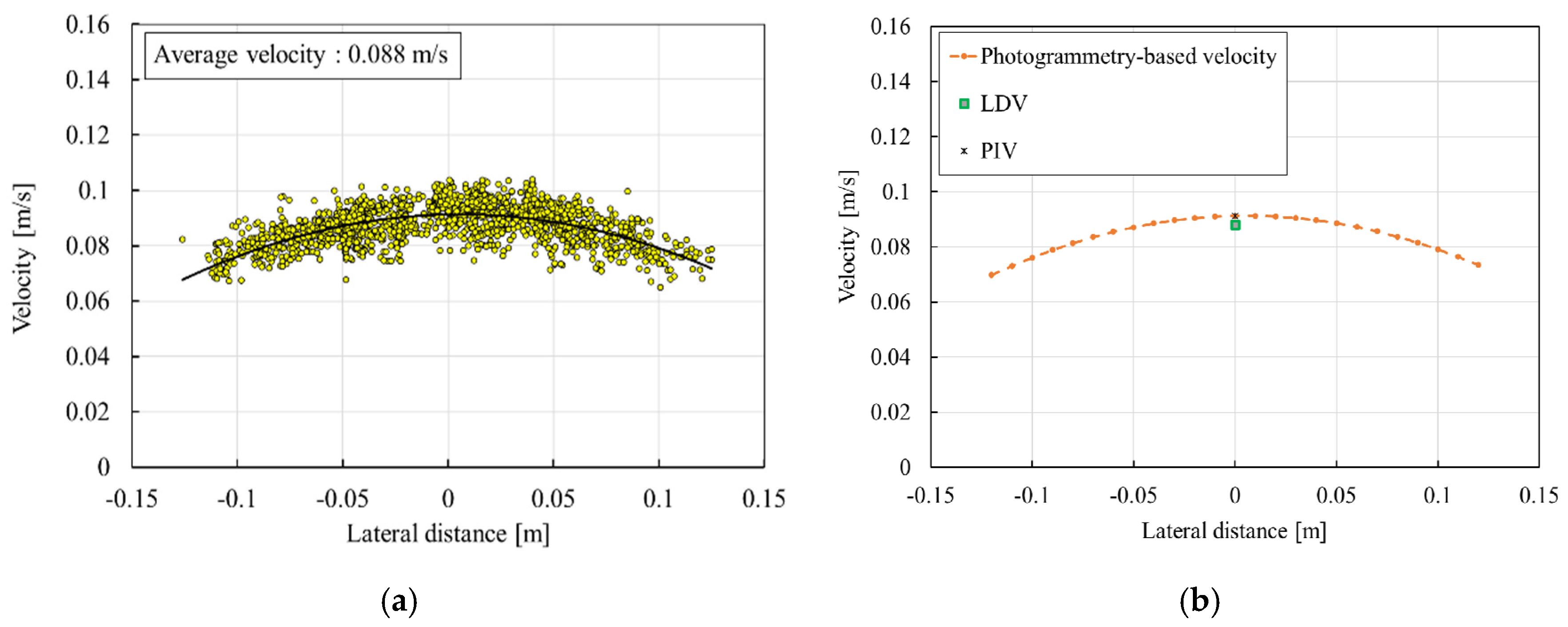
Figure 4 illustrates a velocity field obtained from the data of the laboratory water flume for one set of image sequences. The magnitude of the 3D surface velocity distribution is shown in Figure 5a, with an average velocity value of 88 mm/s. The standard deviation of the measured velocities is found to be 5.5 mm/s. The data points (circles) present velocities of particles, and the trendline is the fitting curve of velocity distribution in the transverse direction. The maximum velocity can be seen at the centerline along the channel.

The experiments were repeatedly conducted at five different times, resulting in five surface velocity profiles to determine the precision of the system. The mean velocity of the five measurements is 89 mm/s, and the standard deviation is estimated to be 7.7 mm/s. The measured velocities along the centerline of the flume are compared to profiles previously measured by PIV and LDV [25], see Figure 5b. The PIV and LDV measurement captured the streamwise mean velocity profile along the centerline of the flume. The nearest locations from the water surface where the velocities can be measure by PIV and LDV were at 30 mm under the water surface. Therefore, only velocity values at these positions from one PIV/LDV were used to compare to surface velocity measured by the photogrammetry. The velocity values measured along the centerline by photogrammetry, PIV, and LDV are found to be 0.0913 m/s, 0.0912 m/s, and 0.0881 m/s, respectively.

5.2. Surface Velocity of the River Reach

The field campaign was carried out on two measurements in two days in a row at the same river reach. The measurement on day 1 is labeled as Measurement 1, and the measurement on day 2 is labeled as Measurement 2. Figure 6 shows the flow velocity and trajectories of particles achieved from data of the field measurements. The average velocities are found to be 1.093 m/s and 1.277 m/s for Measurements 1 and Measurements 2, respectively. The standard deviations of the measurements are found to be 0.062 m/s for Measurement 1 and 0.038 m/s for Measurement 2. Interestingly, the discharge of the river reach can be provided hourly by the data center of the Boden hydropower plant. Therein, at the time while the flow velocity measurements were performed, the river discharges were 495 and 618 m³/s during the time of Measurement 1 and Measurement 2, respectively. The correlation between the photogrammetry-based results and the data provided by the data center can be validated by considering a ratio of Measurement 2 (V₂) to Measurement 1 (V₁), which also involves the change of the river discharges between two measurements. The photogrammetry-based ratio and discharge ratio are 1.17 and 1.25, respectively. At the same river reach, it is assumed that the water stage is lower in Measurement 1 (discharge 495 m³/s) than that in Measurement 2 (discharge 618 m³/s), resulting in a smaller cross-sectional area in Measurement 1 than in Measurement 2, which probably explains some of the difference in these ratios.

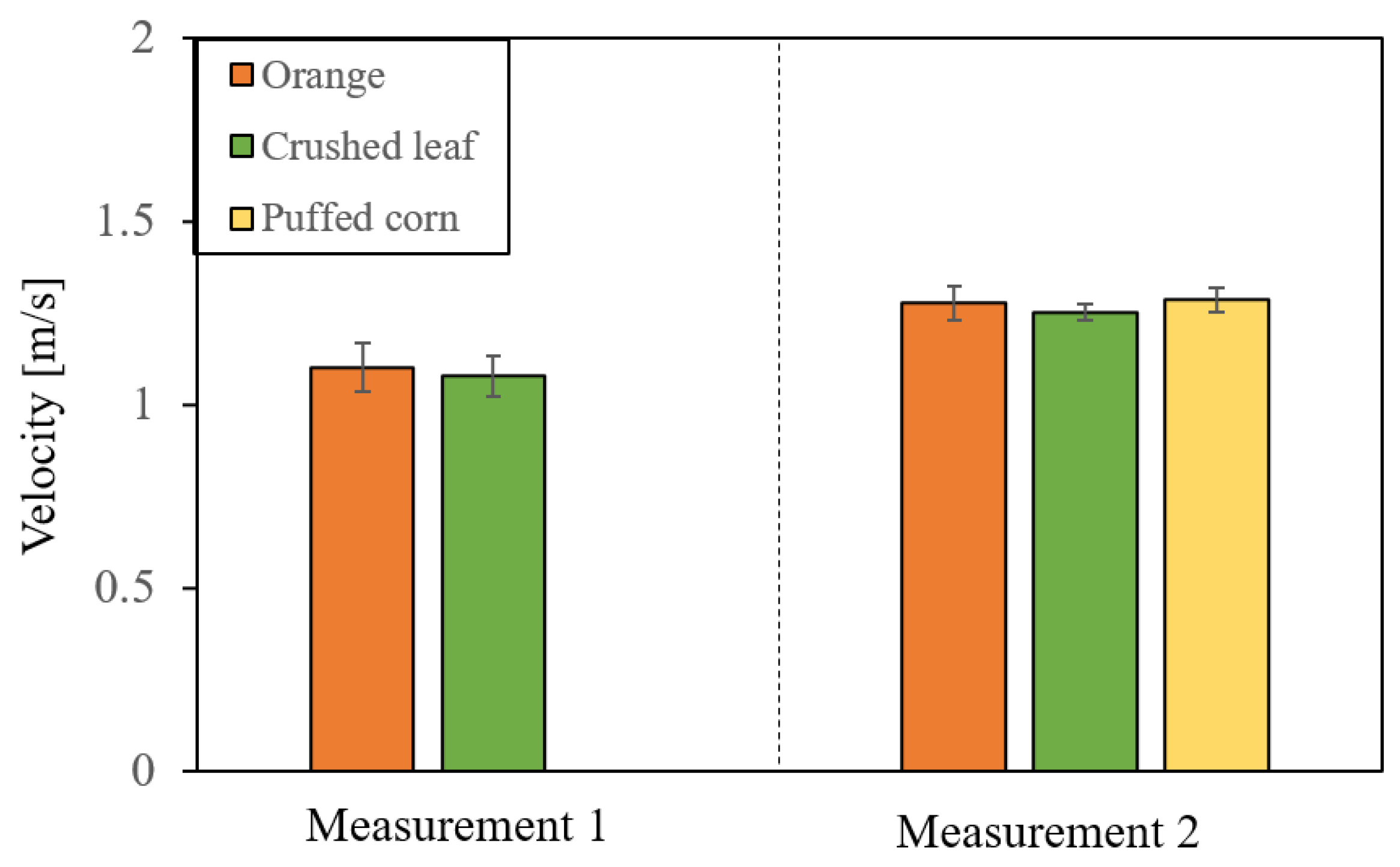
Figure 6 summarizes the trajectories of all types of particles introduced on the free surface. The oranges and crushed leaves were used in Measurement 1. Measurement 2 used puffed corn as an additional tracer beside the oranges and crushed leaves. Considering the average surface velocity measured from each type of particle, Measurement 1 results in 1.091 ± 0.065 m/s and 1.089 ± 0.056 m/s for the oranges and crushed leaves, respectively. These values are 1.276 ± 0.046 m/s, 1.267 ± 0.024 m/s, and 1.269 ± 0.033 m/s, corresponding to the oranges, crushed leaves, and puffed corn particles in Measurement 2, as shown in Figure 7.

5.3. Discussion

The applicability of the photogrammetry-based PTV system for free surface flow velocity measurement was investigated. In order to perform the measurements at natural flow, it is important to study the properties of the measurement system regarding camera setup, camera calibration, and PTV algorithm in a controlled environment. The laboratory measurement was, therefore, conducted for this purpose. The velocities obtained from the different methods were compared. It was seen that the velocities measured along the centerline by photogrammetry, LDV, and PIV agree well with each other. The laboratory investigation revealed that the photogrammetric system is suitable for free surface velocity estimation.

Compared to the single-camera system, the use of the multi-camera system will significantly reduce one of the main PTV-based photogrammetry limitations, which is the image orthorectification before tracking to allow for a correct scaling of the image tracks since such process may lead to interpolation errors [17]. In addition, the multi-camera system enables the estimation of three components of the surface velocity as well as the undulation of the water surface. In this investigation, the main impact of introducing the third surface velocity component was the ensuring of a good velocity estimate over the field of view and the ability to disregard false estimates that appeared far away from the water surface. The third velocity component in the vertical direction gave more information about the shape of the flow, especially in the cases of high flow and nonuniform depth flow.

The precision of the camera calibration contributes an essential part in the accuracy of the measurement, as it plays a significant role in the 3D reconstruction of the particle coordinates. For this reason, the camera calibration process for the field measurement was adjusted to produce a practical procedure that would adapt to the field conditions and ensure that the camera calibration process could be repeated in each measurement. The combination of using commercial software (Agisoft Metashape) for calibration of the intrinsic camera parameters and the self-designed reference frame for the extrinsic parameters results in a simple calibration routine for large-scale measurements, which is one of the most challenging tasks of a photogrammetry-based PTV system.

The measured surface velocities (see Figure 6) indicate the change of the discharges in the river reach at different measurement times; for instance, the flow in Measurement 2 is 15% higher than that in Measurement 1. The corresponding increase reported regarding mass flow through the Boden hydropower plant is 20% for the same measurement times. There is hence a distinct correlation between the local surface velocities measured with photogrammetry and the actual flow through the power plant.

One of the purposes of the paper was to examine the usefulness and compare the results of different types of seeding particles. In the field measurement, the selection of floating particles was made considering the environmental impact, flow characteristics (i.e., water background), the color contrast with respect to the background, and the practice of choice. In this study, all types of selected tracers showed a good level of contrast in clear water conditions. The particle tracking method and pattern tracking method were applied in the PTV algorithm for corresponding features, and both approaches give the results in good accordance regardless of the type of particle (see Figure 7). It is seen that the velocities in Measurement 1 produce a higher deviation than the results obtained in Measurement 2. It might be because of the different wind conditions. The wind speeds were recorded as 3.25 m/s and 2.0 m/s in opposite flow directions during Measurement 1 and Measurement 2, correspondingly.

Regarding the error quantification in the measured velocities, the error sources are split into systematic error and random error. The main error sources in the PIV/PTV considering the entire measurement chain were discussed in [33,34]. In this study, the systematic errors related to the measurement system are estimated from the camera calibration. The random errors, which may be introduced by the instability of the measurement conditions or the flow itself or non-uniformity of the background, are produced from the repetition of the measurements. In the laboratory measurement, the error related to the camera system is about 0.03% on the measured velocities. In the field, these errors in the velocities are estimated to be 1.6% for Measurement 1 and 2.0% for Measurement 2. The random errors are found to be 0.062 m/s and 0.038 m/s for Measurement 1 and Measurement 2, respectively. It can be seen that the random errors are larger than those which are estimated with the errors related to the measurement system, both in the laboratory measurement and in the river flow measurements.

Even if further research is required to study the accuracy of the photogrammetry-based PTV system comprehensively, the investigation in this study demonstrates good potential applicability of using multiple cameras in free surface flow velocity estimation.

6. Conclusions

The multi-camera photogrammetric approach of velocity measurement has been applied for surface velocity estimation of the laboratory water flume to investigate the properties of the camera system and the PTV algorithm in preparation for the field measurements. In the field of view of 0.8 m × 0.8 m (laboratory flume), the error related to the camera system is about 0.03%, while the random error is estimated to be 7.7 mm/s which corresponds to 8.7% on the average velocities. In Measurement 1 at river flow, the error related to the camera system is estimated to be 1.6%, and the random error is about 0.062 m/s which corresponds to 5.7% on the average velocities. These errors are 2.0% and 3.0% for Measurement 2, in the field of view of 11.0 m × 8.2 m. The use of the proposed method can provide a reliable estimation of surface velocity with sufficient accuracy.

The study focuses on the camera calibration processes to improve the accuracy, and to eventually be able to provide a realistic flow surface velocity. The presented calibration routine in the field measurement can help to overcome the challenges while moving out for large-scale and more complex measurement conditions. It, therefore, makes the multiple cameras-based measurement system more practical in natural flow quantification. In addition, two tracking approaches (i.e., the particle tracking and pattern tracking methods) applied in the PTV algorithm can provide flexibility for the field measurement in many circumstances that need tracer seeding due to lack of surface structure on the water flow.

References

- Yorke, T.H.; Oberg, K. Measuring river velocity and discharge with acoustic Doppler profilers. Flow Meas. Instrum. 2002, 13, 191–195. [Google Scholar] [CrossRef]
- Gravelle, R. Discharge Estimation: Techniques and Equipment. In Geomorphological Techniques; Clarke, L.E., Nield, J.M., Eds.; British Society for Geomorphology: London, UK, 2015. [Google Scholar]
- Tauro, F.; Tosi, F.; Mattoccia, S.; Toth, E.; Piscopia, R.; Grimaldi, S. Optical Tracking Velocimetry (OTV): Leveraging Optical Flow and Trajectory-Based Filtering for Surface Streamflow Observations. Remote Sens. 2018, 10, 2010. [Google Scholar] [CrossRef] [Green Version]
- Tauro, F.; Piscopia, R.; Grimaldi, S. PTV-Stream: A simplified particle tracking velocimetry framework for stream surface flow monitoring. Catena 2019, 172, 378–386. [Google Scholar] [CrossRef]
- Tauro, F.; Petroselli, A.; Arcangeletti, E. Assessment of drone-based surface flow observations. Hydrol. Process. 2015, 30, 1114–1130. [Google Scholar] [CrossRef]
- Detert, M.; Johnson, E.D.; Weitbrecht, V. Proof-of-concept for low-cost and non-contact synoptic airborne river flow measurements. Int. J. Remote Sens. 2017, 38, 2780–2807. [Google Scholar] [CrossRef]
- Fujita, I.; Muste, M.; Kruger, A. Large-scale particle image velocimetry for flow analysis in hydraulic engineering applications. J. Hydraul. Res. 1998, 36, 397–414. [Google Scholar] [CrossRef]
- Aya, S.; Kakinoki, S.; Aburaya, T.; Fujita, I.; Wada, A.; Ninokata, H.; Tanaka, N. Velocity and turbulence measurement of river flows by lspiv. In Advances in Fluid Modeling and Turbulence Measurements; World Scientific Pub Co Pte Lt: Singapore, 2002; pp. 177–184. [Google Scholar]
- Muste, M.; Xiong, Z.; Schöne, J.; Li, Z. Validation and Extension of Image Velocimetry Capabilities for Flow Diagnostics in Hydraulic Modeling. J. Hydraul. Eng. 2004, 130, 175–185. [Google Scholar] [CrossRef]
- Meselhe, E.A.; Peeva, T.; Muste, M. Large Scale Particle Image Velocimetry for Low Velocity and Shallow Water Flows. J. Hydraul. Eng. 2004, 130, 937–940. [Google Scholar] [CrossRef]
- Fujita, I.; Watanabe, H.; Tsubaki, R. Development of a non-intrusive and efficient flow monitoring technique: The space-time image velocimetry (STIV). Int. J. River Basin Manag. 2007, 5, 105–114. [Google Scholar] [CrossRef] [Green Version]
- Perks, M.T.; Russell, A.J.; Large, A.R.G. Technical Note: Advances in flash flood monitoring using unmanned aerial vehicles (UAVs). Hydrol. Earth Syst. Sci. 2016, 20, 4005–4015. [Google Scholar] [CrossRef] [Green Version]
- Khalid, M.; Pénard, L.; Mémin, E. Optical flow for image-based river velocity estimation. Flow Meas. Instrum. 2019, 65, 110–121. [Google Scholar] [CrossRef] [Green Version]
- Lloyd, P.M.; Stansby, P.K.; Ball, D.J. Unsteady surface-velocity field measurement using particle tracking velocimetry. J. Hydraul. Res. 1995, 33, 519–534. [Google Scholar] [CrossRef]
- Brevis, W.; Niño, Y.; Jirka, G.H. Integrating cross-correlation and relaxation algorithms for particle tracking velocimetry. Exp. Fluids 2011, 50, 135–147. [Google Scholar] [CrossRef]
- Sasso, S.F.D.; Pizarro, A.; Samela, C.; Mita, L.; Manfreda, S. Exploring the optimal experimental setup for surface flow velocity measurements using PTV. Environ. Monit. Assess. 2018, 190, 460. [Google Scholar] [CrossRef] [PubMed]
- Eltner, A.; Sardemann, H.; Grundmann, J. Technical Note: Flow velocity and discharge measurement in rivers using terrestrial and unmanned-aerial-vehicle imagery. Hydrol. Earth Syst. Sci. 2020, 24, 1429–1445. [Google Scholar] [CrossRef] [Green Version]
- Fuchs, T.; Hain, R.; Kähler, C.J. Non-iterative double-frame 2D/3D particle tracking velocimetry. Exp. Fluids 2017, 58, 119. [Google Scholar] [CrossRef]
- Tauro, F.; Piscopia, R.; Grimaldi, S. Streamflow Observations from Cameras: Large-Scale Particle Image Velocimetry or Particle Tracking Velocimetry? Water Resour. Res. 2017, 53, 10374–10394. [Google Scholar] [CrossRef] [Green Version]
- Kim, J.; Muste, M.; Hauet, A.; Krajewski, W.F.; Kruger, A.; Bradley, A. Stream discharge using mobile large-scale particle image velocimetry: A proof of concept. Water Resour. Res. 2008, 44. [Google Scholar] [CrossRef]
- Chandler, J.; Ferreira, E.; Wackrow, R.; Shiono, K. Water Surface and Velocity Measurement-River and Flume. ISPRS Int. Arch. Photogramm. Remote Sens. Spat. Inf. Sci. 2014, XL-5, 151–156. [Google Scholar] [CrossRef] [Green Version]
- Hoshino, T.; Yasuda, H. 3D Measurement of Water and Bed Surface Shapes during the Formation of Sand Waves Using the Moving Optical Cutting Method. In Proceedings of the 12th International Conference on Hydroscience & Engineering, Hydro-Science & Engineering for Environmental Resilience, Tainan, Taiwan, 6–10 November 2016. [Google Scholar]
- Li, W.; Liao, Q.; Ran, Q. Stereo-imaging LSPIV (SI-LSPIV) for 3D water surface reconstruction and discharge measurement in mountain river flows. J. Hydrol. 2019, 578, 124099. [Google Scholar] [CrossRef]
- Luhmann, T. Close range photogrammetry for industrial applications. ISPRS J. Photogramm. Remote Sens. 2010, 65, 558–569. [Google Scholar] [CrossRef]
- Bin Asad, S.M.S. Laser Based Flow Measurements to Evaluate Hydraulic Conditions for Migrating Fish and Benthic Fauna. Ph.D. Thesis, Luleå University of Technology, Luleå, Sweden, 2019. [Google Scholar]
- De la Escalera, A.; Armingol, J.M. Automatic chessboard detection for intrinsic and extrinsic camera parameter calibration. Sensors 2010, 10, 2027–2044. [Google Scholar] [CrossRef] [PubMed]
- Bok, Y.; Ha, H.; Kweon, I.S. Automated checkerboard detection and indexing using circular boundaries. Pattern Recognit. Lett. 2016, 71, 66–72. [Google Scholar] [CrossRef]
- Matas, J.; Chum, O.; Urban, M.; Pajdla, T. Robust wide-baseline stereo from maximally stable extremal regions. Image Vis. Comput. 2004, 22, 761–767. [Google Scholar] [CrossRef]
- Nistér, D.; Stewénius, H. Linear Time Maximally Stable Extremal Regions. In Transactions on Petri Nets and Other Models of Concurrency XV; Springer: Berlin/Heidelberg, Germany, 2008; pp. 183–196. [Google Scholar]
- Song, X.; Yamamoto, F.; Iguchi, M.; Murai, Y. A new tracking algorithm of PIV and removal of spurious vectors using Delaunay tessellation. Exp. Fluids 1999, 26, 371–380. [Google Scholar] [CrossRef]
- Ruhnau, P.; Guetter, C.; Putze, T.; Schnorr, C. A variational approach for particle tracking velocimetry. Meas. Sci. Technol. 2005, 16, 1449–1458. [Google Scholar] [CrossRef] [Green Version]
- Bergström, P.; Edlund, O. Robust registration of point sets using iteratively reweighted least squares. Comput. Optim. Appl. 2014, 58, 543–561. [Google Scholar] [CrossRef]
- Wieneke, B. PIV Uncertainty Quantification and Beyond; Delft University Press: Delft, The Netherlands, 2017. [Google Scholar]
- Sciacchitano, A. Uncertainty quantification in particle image velocimetry. Meas. Sci. Technol. 2019, 30, 092001. [Google Scholar] [CrossRef] [Green Version]
Figure 1.
Laboratory flume measurement setup: (a) Sketch of the surface velocity measurement setup; (b) Checkerboard pattern for calibration; (c) Wooden bead particle.
Figure 2.
Location of the field measurement campaign—Svedjebron, Boden, Sweden (Google maps).
Figure 3.
Field measurements setup and camera calibration: (a) River flow measurement setup; (b) Natural pattern for intrinsic camera calibration (Agisoft Metashape); (c) Reference wooden frame for extrinsic camera calibration.
Figure 4.
Surface flow velocity field of the laboratory flume measurement.
Figure 5.
Surface velocity distribution in transverse direction: (a) Distribution of surface velocity and fitting curve. The circles present velocities of particles; (b) Comparison velocity profiles.
Figure 6.
Surface velocity of the field measurements: (a) Measurement 1 (Record time: 3.50 s); (b) Measurement 2 (Record time: 3.70 s).
Figure 7.
Surface velocity by different particle types.
Publisher’s Note: MDPI stays neutral with regard to jurisdictional claims in published maps and institutional affiliations. |
© 2021 by the authors. Licensee MDPI, Basel, Switzerland. This article is an open access article distributed under the terms and conditions of the Creative Commons Attribution (CC BY) license (https://creativecommons.org/licenses/by/4.0/).
Share and Cite
MDPI and ACS Style
Trieu, H.; Bergström, P.; Sjödahl, M.; Hellström, J.G.I.; Andreasson, P.; Lycksam, H. Photogrammetry for Free Surface Flow Velocity Measurement: From Laboratory to Field Measurements. Water 2021, 13, 1675. https://doi.org/10.3390/w13121675
AMA Style
Trieu H, Bergström P, Sjödahl M, Hellström JGI, Andreasson P, Lycksam H. Photogrammetry for Free Surface Flow Velocity Measurement: From Laboratory to Field Measurements. Water. 2021; 13(12):1675. https://doi.org/10.3390/w13121675
Chicago/Turabian StyleTrieu, Hang, Per Bergström, Mikael Sjödahl, J. Gunnar I. Hellström, Patrik Andreasson, and Henrik Lycksam. 2021. "Photogrammetry for Free Surface Flow Velocity Measurement: From Laboratory to Field Measurements" Water 13, no. 12: 1675. https://doi.org/10.3390/w13121675
Note that from the first issue of 2016, this journal uses article numbers instead of page numbers. See further details here.