
Effects of Topography on Planted Trees in a Headwater Catchment on the Chinese Loess Plateau


1
State Key Laboratory of Loess and Quaternary Geology, Institute of Earth Environment, Chinese Academy of Sciences, Xi’an 710061, China
2
University of Chinese Academy of Sciences, Beijing 100049, China
3
CAS Center for Excellence in Quaternary Science and Global Change, Xi’an 710061, China
*
Author to whom correspondence should be addressed.
Forests 2021, 12(6), 792; https://doi.org/10.3390/f12060792
Submission received: 13 May 2021
/
Revised: 11 June 2021
/
Accepted: 13 June 2021
/
Published: 16 June 2021
(This article belongs to the Section Forest Inventory, Modeling and Remote Sensing)
Abstract
:The Chinese Loess Plateau (CLP) is known for its complex topography of hills and gullies, and lots of human land-use management activities have been put into practice to sustain the soil, water and other natural resources. Afforestation has been widely applied on the CLP and it’s important to understand the effects of topography on these planted trees. However, the coarse spatial resolution of remote sensing data makes it insensitive to local topography, and the traditional in-situ measurements would consume vast amounts of time and resources. In this study, a small headwater catchment of the CLP was selected to study the effects of topography on the planted trees. Low altitude unmanned aerial vehicle based light detection and ranging (UAV-based LiDAR) technology was utilized to obtain high-resolution topography and vegetation structure data. Results showed that the middle transition zone (mid-transition, slope > 45°) was an important boundary of topography in the gully area of the CLP. In the forested catchment, the area of the mid-transition zone had the lowest of tree density, canopy coverage and leaf area index due to steep slope gradient. The tall trees ten to twenty meters high were concentrated in the downhill area, which had the highest canopy coverage and leaf area index. Elevation had significant linear relationships with canopy coverage and leaf area index (p < 0.001), which revealed the impact of topography on the forest indexes of the afforestation catchment. We concluded that the high-resolution LiDAR technology facilitated the research of topography and forest interactions in land surface.
1. Introduction
The topography has a significant influence on the growth and distribution of trees and they co-evolve under the joint influences of climate and the local ecosystems [1]. The differentiations of energy and moisture controlled by topography are the core factors driving the evolution of trees distribution under natural conditions [2,3]. Previous studies that characterized the interactions between topography and trees have been mostly conducted at basin or plot scale [4,5,6]. Headwater catchment is the basic geomorphic unit in studying the interactions of Earth surface processes, climate change and human impacts [2]. Thus, precise characterization of the relationship between topography and trees in headwater catchments can provide an in-depth understanding of microtopography impacts on trees growth and distribution.
Afforestation is widely used to restore deteriorated ecosystems and combat land desertification in many places of the world. However, if looking back upon the arduous development of afforestation in the past twenty years, it has been and continues to be a controversial topic that keeps sparking academic and social debates [7,8,9,10,11,12]. The afforestation of drylands is criticized for its negative impact on water resources. On the other hand, many studies have shown that afforestation is more efficient in flood control and soil erosion reduction than the natural regrowth of grassland in some arid and semiarid regions, especially during the early stages of ecosystem rehabilitation [13,14,15]. Moreover, properly managed forest ecosystems play an important role in the progress towards meeting carbon neutrality targets, not just in China, but all over the world [16,17,18,19]. The satellite data (2000–2017) reveals that the afforestation and cultivation of China and India lead the greening of the world, and the afforestation in China alone accounts for 10.5% of the global net increase in leaf area [20]. It is known that the afforestation work should be managed according to the topographic diversity, local climate, soil conditions and available resources. In reality, the topographic diversity plays an important role in the evolution of habitat diversity with its power in the determination of local thermal, humidity, and soil fertility conditions, and that should be taken into account when selecting reasonable species for afforestation, considering its potential strength to increase the ecological stability as well as to support the forestry productivity [21]. Also, the topographic concavity creates climatic microrefugia for local species, and the differentiation of the microtopographic thermal and moisture conditions can impact the species redistribution [3,22,23]. In the past, forest inventories were generally used to obtain quantitative information about trees. However, such manual methods are not efficient due to their need for a large labor force. Moreover, it is also difficult to obtain high-resolution topography data through traditional methods, and thus, it is a challenge to quantitively and precisely characterize the relationship between topography and trees.
In recent years, high technologies, such as the small low-altitude unmanned aerial vehicle (UAV), digital aerial photogrammetry (DAP), light detection and ranging (LiDAR) and aerial laser scanning (ALS) techniques have been widely applied to quantify the high-resolution data of topography and trees due to their advantages of high flexibility and high efficiency [24,25,26]. It’s suggested that affordable and portable UAV-borne LiDAR system can generate very high resolution three-dimensional (3D) habitat information, including terrain and vegetation structure [27]. For example, Grijseels et al. [28] utilized LiDAR imaging and found that the riparian vegetation structure follows the patterns of topography related to energy and water subsidies; Cucchiaro et al. [29] combined the 3D photogrammetry and terrestrial LiDAR scanning (TLS) techniques and concluded that this data fusion can be utilized to create highly accurate digital terrain models (DTMs) in the context of complex and unreachable topography and vegetation cover. The high-resolution UAV and LiDAR techniques facilitate the observation practice of geomorphic change characterization [30]. Meinen and Robinson utilized UAV collected time-series data in the evaluation of soil erosion models in field experiments [31]. Gong et al. [32] applied the UAVs and structure from motion (SfM) technology to obtain high-resolution three-dimensional models of the erosion gully in an open-pit coal mine, and the freeze-thaw cycle- caused soil erosion was clearly captured. Thus, the integrated method of LiDAR and 3D photogrammetry has provided new possibilities to comprehensively quantify the relationship between the topography and vegetation distribution.
The Chinese Loess Plateau (CLP) is a semi-arid region characterized by extensive loess distribution, low vegetation coverage, and severe soil erosion [33,34,35]. Since 1991, the Chinese government has launched the ‘Conversion of Cropland to Forest Program’ (CCFP), also known as the ‘Grain for Green’ project, and this project pays farmers to restore their farmland and the degraded land to forest, shrub and grassland [36,37]. After nearly 20 years of rehabilitation efforts, 16,000 km2 of rain-fed cropland has been converted back into planted vegetation, which has caused a 25%–28% increase in vegetation coverage on the CLP [10,38,39]. Some studies have demonstrated that this large-scale afforestation and crop plantation on the CLP has induced a decline in both blue and green water resources, which would result in the degradation of forest ecosystems and the mosaic distribution of vegetation due to the microtopography impacts [11,40,41,42]. However, the precise relationship between topography and trees in headwater catchments on the CLP is underestimated due to the limitations of current technology. The lack of such information will hinder our understanding of the evolution of planted trees and their relationship with the landform in the catchment.
We hypothesize that topography should have a significant impact on the spatial distribution of planted trees at catchment scale. To test this hypothesis, a planted headwater catchment was selected to study the influence of topography on the evolution of trees. The catchment was planted in 1954 [5] and almost 90% was replanted with the single tree species Robinia pseudoacacia Linn. A small number of other tree species were planted along the edge of the catchment. Thus, the catchment can be treated as a monoculture catchment with singular tree species of R. pseudoacacia. Moreover, the catchment has more than 60 years of afforestation history, which can provide a predictive information for the evolution and adaption of trees at catchment scale on the CLP.
In this study, the high-resolution data of forest indexes and topography in the catchment were obtained using the techniques of DAP and UAV-borne LiDAR and their relationships were deeply analyzed. The objectives of this study were to: (1) quantify the high-resolution spatial information of the landform and tree distributions, and (2) characterize the relationships between the topography and forest indexes at catchment scale.
2. Materials and Methods
2.1. Study Area
This study was conducted in a headwater catchment (Yangjiagou) on the southern CLP (107°33′19″ E, 35°41′52″ N). The small headwater catchment has an area of 0.87 km2, and it locates in the Nanxiaohegou basin of Xifeng district, Qingyang city, Gansu province, China (Figure 1). It is a typical loess tableland and gully area, and the altitude ranges from 1180 m to 1365 m based on the ASTER GDEM V2 data. The mean annual temperature is 9.3 °C and the mean annual precipitation is 556.5 mm, and more than two thirds of annual precipitation occurred from June to September [43]. The loessal soil in the catchment derives from the Quaternary dust and it’s about 200–250 m thick with the texture mostly of silt-loamy [5,44,45,46]. The studied (Yangjiagou) catchment is generally composed of three basic landform units, including the level ground, upper hillslope, and down slope gully. The level ground is a flat area with a slope lower than 5 degrees, and it’s used for cultivation which include wheat and corn plantation. The upper hillslope with a gentle slope gradient (10° to 20°) connects the tableland and the down slope gully. The down slope gully with steep gradient is covered with high density of trees and understory vegetation [43].
Before 1954, the soil erosion processes in the catchment were dominated by hillslope water erosion and gully gravity erosion due to farming activities. In 1954–1958, the afforestation project was deployed in the catchment and surface and gravity erosion significantly decreased. After 65 years of vegetation restoration, soil erosion is completely controlled. Although gully gravity erosion occasionally occurred, the sediments cannot deliver to the outlet of the catchment due to the strong control effects of gully trees and understory. In 1954–1958, almost the total area of the catchment was planted with the single tree species of R. pseudoacacia. In the later time, a small number of other tree species, e.g., Armeniaca sibirica (L.) Lam, Pinus tabuliformis Carr., Salix matsudana Koidz., and Platycladus orientalis (L.) Franco, are planted in the edge of the catchment and their distribution area is less than 10%. Since 1954, cultivating, grazing, and lumbering were forbidden in the area until present day [5,43]. After 65 years of evolution, the catchment now forms a stable forest ecosystem [5,44,47]. In April of 2019, we conducted a carefully field investigation in the catchment and found that the planted trees of R. pseudoacacia account for almost 90% area of the catchment, and most of them are big trees with the height of 10 to 20 m and prosperous canopy. The tree species of A. sibirica, P. tabuliformis, S. matsudana, and P. orientalis are scattered along the edge of the catchment. Thus, the studied catchment can be treated as a monoculture catchment. During the past 60 years, the planted catchment received no large-scale forestry work, such as thinning. Currently, the trees (including understory vegetation) and hydrology in the gully have evolved into a natural equilibrium [5,43,48], thus making it an ideal case to study the effects of topography on the spatial distribution of trees at catchment scale on the CLP.
2.2. Field Investigation and Aerial Scanning
Figure 2 shows the workflow of characterizing the effects of topography on trees in the Yangjiagou forest catchment. The ASTER GDEM V2 DEM and QuickBird images were used in the initial exploration of the Yangjiagou forest catchment in the summer of 2018. The ASTER GDEM V2 DEM images (30 m × 30 m) were firstly used to establish the rough outline of the altitude background of the study area, and the data set was provided by Geospatial Data Cloud site, Computer Network Information Center, Chinese Academy of Sciences. (http://www.gscloud.cn, accessed on 1 January 2018). The QuickBird multispectral images (2 m × 2 m), which were obtained from the company Digital Globe (https://www.digitalglobe.com, accessed in 1 February 2018), were then applied to depict the catchment landform. After that image exploration in 2018 summer, a UAV-based DAP flight was carried out in the Yangjiagou catchment in September 2018. The reconstructed high-resolution 3D model of the DAP result facilitated our next field investigation and ALS flight planning, which were deployed in 2019. We collaborated with the local authority of forestry management (the Xifeng Supervision Bureau of Soil and Water Conservation), and we commenced a large field investigation of topography and vegetation during the April of 2019.
The DAP flight was carried out in the September of 2018. The low-altitude DAP system consists of a Phantom 4 Pro drone (DJI, https://www.dji.com, accessed on 15 June 2021) equipped with a 20-megapixel digital camera and related power and communication accessories. The Phantom 4 Pro was used to take series of flight attitude information-embedded high-resolution photos, with 40% coverage of the adjacent pictures in both the vertical and horizontal directions. Those pictures were spatially aligned, orthorectified, mosaic processed, and transformed into digital surface models (DSM) and orthoimages by using the Agisoft PhotoScan 1.4 software (now renamed Agisoft Metashape, https://www.agisoft.com/, accessed on 1 January 2018). The precise boundary of the study area was obtained based on the high-resolution orthoimages and DSM and careful field investigation, which facilitated the consequent ALS flight plan.
The ALS flight was deployed in July 2019, when the rainy season was about to begin and the vegetation started to prosper. The UAV-based LiDAR system is an integrated light-weight aerial Light Detection and Ranging (LiDAR) synthesis, consisted of a DJI M600 Pro drone with the real-time kinematic (RTK) mobile station and a LiAir 220 LiDAR system from Beijing Green Valley Technology. Co., Ltd. (https://www.lidar360.com/, accessed on 1 January 2018). This platform could work 30 min in the air and the longest range was about 200 m with a resolution of ±2 cm at the 20% reflectivity. Since the high-density laser beam of LiDAR could penetrate the plant canopy and both canopy and understory landform information can be obtained. The LiDAR360 software, which is a professional LiDAR point cloud processing and analyzing software developed by Beijing Green Valley Technology. Co., Ltd., were used to process the high-resolution data of both forest and landform. After a preliminary work of point cloud outlier removement, ground points classification, noise filter, ground points normalization, boundary extraction and subsampling, the resulting point cloud was utilized in the subsequent calculation of topographic and forest indexes.
2.3. Topographical and Forest Indexes
2.3.1. Topographical Indexes
A digital elevation model (DEM) of the Yangjiagou forest catchment was generated from the preprocessed point cloud by using the terrain toolbox in LiDAR360, with a pixel size of 0.5 × 0.5 m. The basic topographical indexes, including elevation, slope, and aspect, were calculated using spatial analyst tools in ArcGIS 10.6, and the other two indexes, topographic wetness index (TWI) and direct insolation (DI) were computed in SAGA 7.5.0 (http://www.saga-gis.org/, http://saga-gis.sourceforge.net/en/, accessed on 1 January 2018) [49].
Based on an integrative analysis of slope distribution and in-situ investigation, four classes of slopes in the Yangjiagou forest catchment were defined: (1) slopes lower than 10° (gentle slopes); (2) slopes ranging from 10° to 25° (middle slopes), (3) slopes ranging from 25°to 45° (steep slopes with significant surface erosion), and (4) slopes higher than 45° (precipitous slopes with significant gravity erosion).
TWI is one of the most widely used topographic indexes, which is related to the spatial distribution and size of saturation zones or variable source areas for runoff generation [50,51,52]. TWI is calculated from specific catchment area (α) of upper slope and local slope (tanβ) [53]. In this study, the standard computing method of TWI was applied, which calculated based on the equation of ln(α/tanβ) [50,52]. Direct insolation (DI) is the potential incoming solar radiation of a certain area in a specified time range, and the index of DI in this study was calculated using the Terrain Analysis tools in SAGA 7.5.0. The scenario period was set from February 1st, 2019 to December 31st, 2019 with the resolution of 7 days, and the whole day was set as the time span with a resolution of 0.5 h.
2.3.2. Forest Indexes
Canopy height model (CHM) is defined as the average height of the top of the vegetated canopy. Canopy cover (CC) is defined as the vertical projection of the tree canopy onto a hypothetical horizontal surface ground. Leaf area index (LAI) is the ratio of total upper leaf surface area to ground area (for broadleaf trees), or total projected conifer needle surface area to ground area (for coniferous plants). LAI directly represents the canopy structure and impacts the energy exchange, evapotranspiration and carbon dioxide between plants and atmosphere, which can be used to predict primary productivity and crop growth [54]. Tree density (TD) is the number of trees in a given area, which is convenient and intuitive to display the plantation status. Since the default and smallest output pixel size of LAI was 15 m × 15 m, the TD, CHM, and CC were resampled and adjusted to the same pixel size as above. In this study, the minimum tree height was set as 2 m and crown base height threshold was set 0.8 m. The indexes of CHM, CC and LAI were calculated using the ALS Forest toolbox in LiDAR360 [55] and TD was calculated based on the spatial coordinates of trees from the forest segmentation data.
2.4. Statistical Analysis
The topographical and forest indexes were spatially aligned and converted from raster into matrix data, so that the significance test (Wilcoxon test), correlation analysis (Pearson method), and linear regression can be performed to quantify the relationships between the landform and vegetation. All the statistical analysis was conducted in the RStudio software (version1.2.5019, http://www.rstudio.com/, accessed on 1 July 2018) with R (version 3.6.2, https://www.R-project.org/, accessed on 1 July 2018) [56,57].
The topography and forest indexes were point-to-point aligned and transformed into unified raster data with the pixel size of 15 m × 15 m, then converted into points (observations). The elevation of the forest catchment was replaced with the relative elevation, which was the result of elevation minus the lowest altitude in Yangjiagou forest catchment. The observations were then utilized in the subsequent significance test, correlation analysis, and linear regression. The Wilcoxon test (α = 0.05) [58,59] were used and the comprehensively integrated observations were measured to verify the differences of topographical and forest data among the paired slope classes. The null hypothesis was that the paired slope classes have the same data distribution of topographical or forest index, and the alternative hypothesis was that the paired slope classes are different in the topographical or forest data distribution.
3. Results
3.1. Topographical Features of the Headwater Catchment
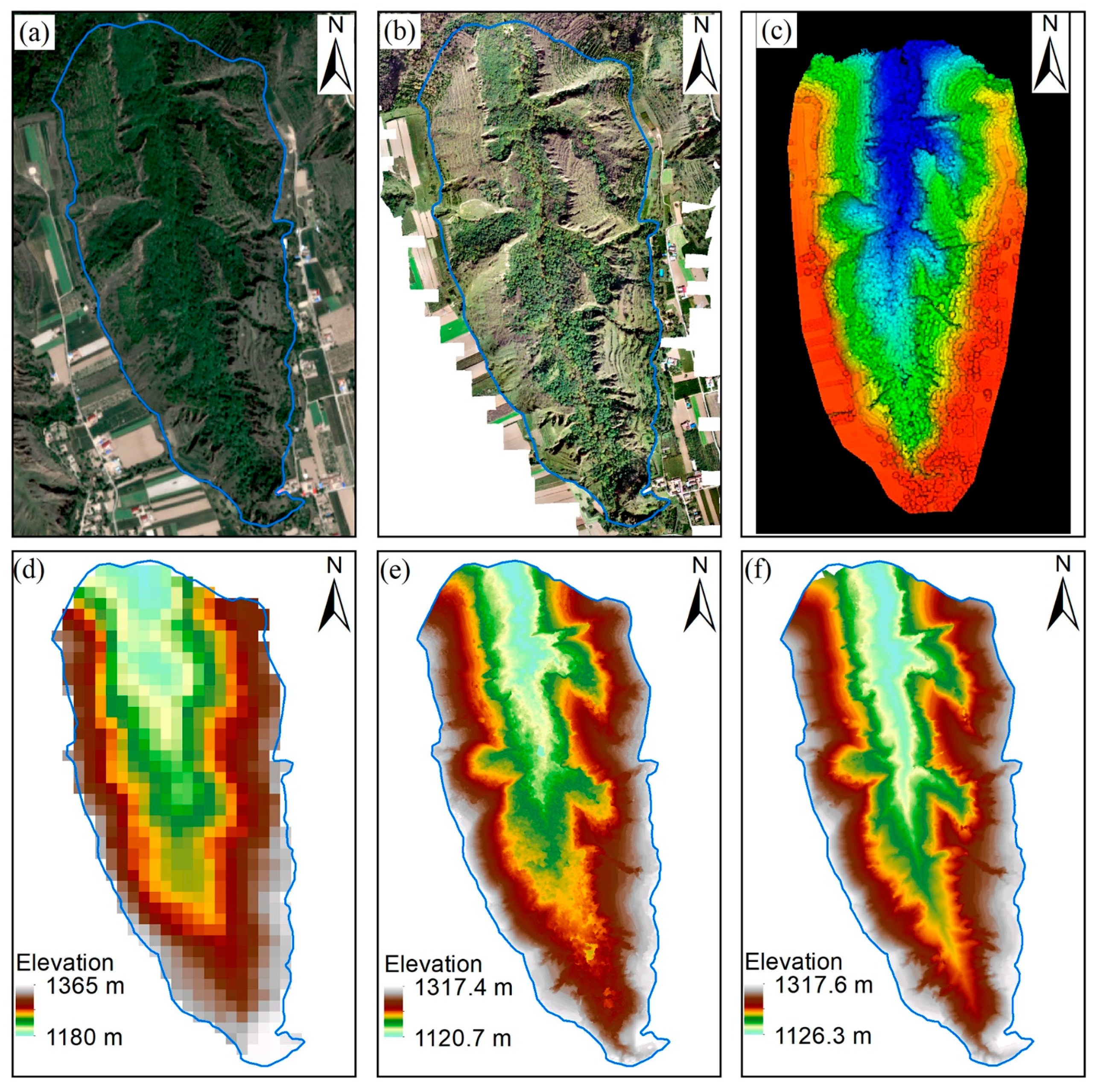
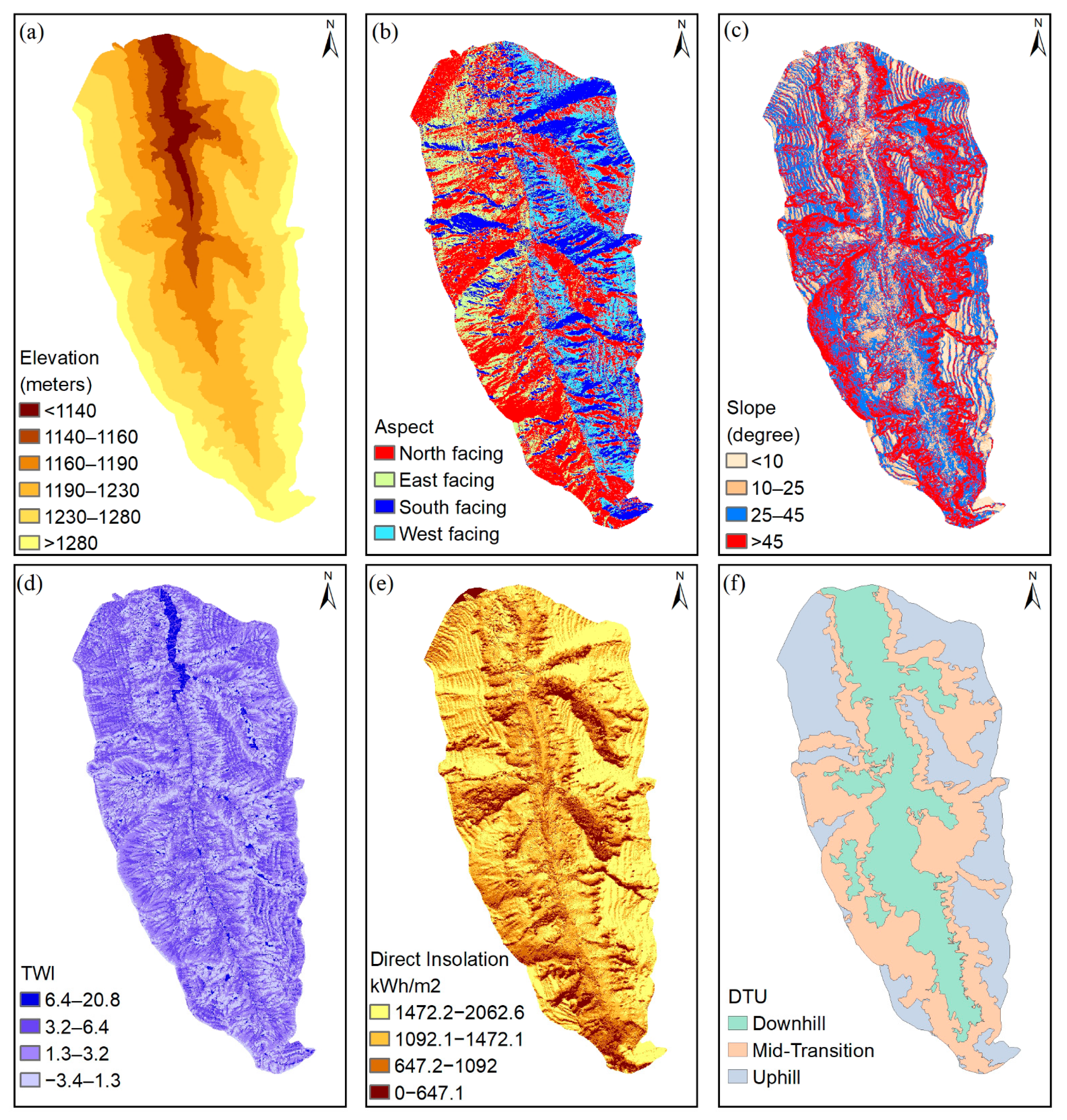
Compared with the images of QuickBird, ASTER GDEM and DAP, the LiDAR imagery showed the highest accuracy of vegetation and landform information (Figure 3). As a result, the spatial distribution of elevation, aspect, slope, TWI and direct insolation was calculated based on the ALS point cloud data (Figure 4). The elevation of the Yangjiagou forest catchment ranges from 1126.3 to 1317.6 m, which can be categorized into six classes: <1140 m (the lowest part of the gully bottom), 1140–1160 m (the gully bottom), 1160–1190 m (the lower slope), 1190- 1230 m (the middle slope), 1230–1280 m (the higher slope), and >1280 m (the edge of loess tableland) (Figure 4a). In the forest catchment, the north, east, south and west facings occupied 22.7%, 32.3%, 11.5%, and 33.5% of the catchment area, respectively (Figure 4b), and the insolation showed clear aspect-dependent patterns (Figure 4e). The south facing slope received 30–100% more insolation than the north facing slope during the study year of 2019. The slope of the forest catchment showed four clear classes (<10°, 10°–25°, 25°–45° and >45°) (Figure 4c) and the simulated TWI also showed slope-dependent patterns (Figure 4d). Figure 4c revealed an obvious boundary between the upper part and the lower part, which were significant different in slope and elevation. These three sections of particular topographic positions could be regarded as three different landform units: the downhill slope, the middle transition zone (slope > 45°), and the uphill slope, hence it was named as the DTU landform system (Figure 4f).
3.2. Forest Indexes of the Headwater Catchment
Based on the field investigation results, we assume that the other tree species located in the catchment boundary cannot have obvious impacts on the distribution of forest indexes at catchment scale. Moreover, the planted catchment did not receive any forestry work, such as thinning. Thus, the characterized relationships between topography and forest indexes in the catchment is reliable.
Figure 5 shows the distribution of forest indexes of the studied catchment. The average density of trees in the forest catchment was 8.6 stems per 225 m2. The downstream revealed a relatively higher density of trees than that in the upper stream. Moreover, the upper hillslope showed relatively higher density of trees than that in the down slope, especially in the downstream of the catchment. The canopy height of trees ranged from 3 to 10 m in the upper hillslope and the middle transition zone areas. Most of the tall trees concentrated in the down slope of the catchment, which shows the height of 10–20 m. The diameter at breast height of those trees ranged from 0.3 to 0.6 m. The CC and LAI showed significant higher values in the down slope than that in other areas. The average CC of the catchment was about 60–70%, and the down slope showed obviously higher CC than the other landforms. The values of LAI in the down slope were generally higher than 1 and the other areas were mostly lower than 1.
3.3. Slope-Dependent Differences of Topography and Forest Indexes
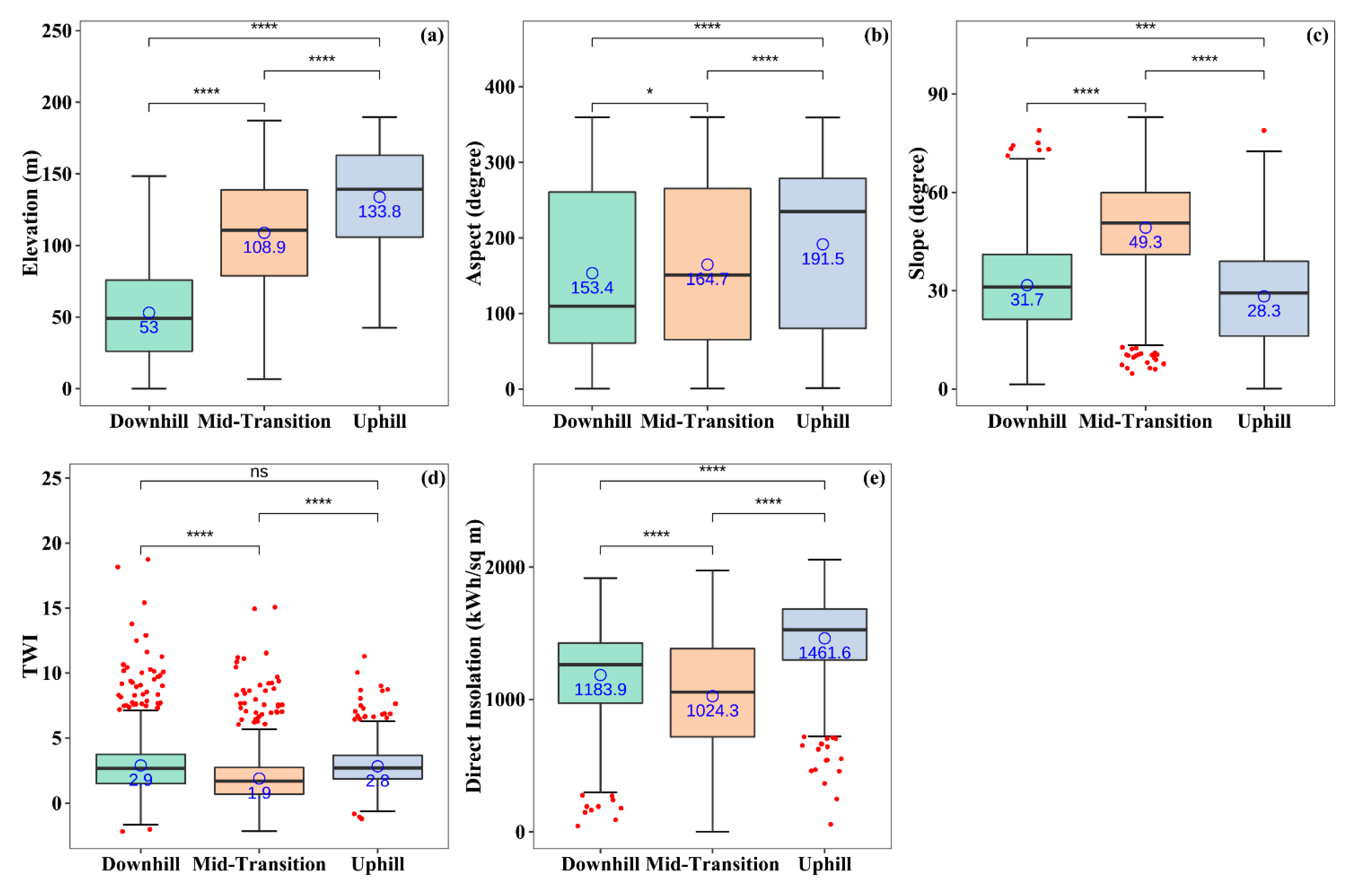
In this study, the topography and forest indexes in the Yangjiagou catchment were converted into 2540 vector points and the Wilcoxon test (α = 0.05) was used to verify the differences of topographical and forest indexes among the three different landform units, uphill slope, middle transition zone, and the downhill slope (Figure 6 and Figure 7). The distributions of elevation, aspect, slope and direct insolation were significantly different among the three different landform units (p < 0.0001, Figure 6). Moreover, the TWI was also different between the uphill and downhill slope (p < 0.0001, Figure 6). In the Yangjiagou forest catchment, the average elevation differences of the downhill, mid-transition and uphill slope were 53.0, 108.8 and 133.8 m, respectively. The aspect of the uphill slope was significantly different from that of the mid-transition and downhill slope, which showed a wide area of insolation in the upper hill. The average slopes of the downhill, mid-transition, and uphill, were 31.7°, 49.3° and 28.3°, respectively.
The distributions of TD, CHM, CC and LAI were significantly different among the three different landform units (p < 0.0001). TD in the middle transition zone was significantly different from the uphill and downhill slopes (p < 0.001, Figure 7). However, no significant differences were found for TD between the upper and down slope areas. The average TD in the middle transition zone was 8.1 stems per 225 m2, which was lower than 9.1 in the downhill slope and 8.8 in the uphill slope. The CHM, CC and LAI showed a decreasing trend from the gully bottom to the upper hills (Figure 7). The average canopy heights in the three different landform units (downhill, mid-transition, uphill) were 8.5, 3.3 and 2.4 m, respectively, and the highest tree of 25.3 m occurred in the down slope area. The average CC in the three different landform units were 79.5%, 50.7%, and 45.4% and the average LAI were 0.99, 0.42, and 0.35, respectively, indicating that the downhill slope area has good moisture conditions for tree growth.
3.4. Correlation and Linear Regression Analysis of Topography and Forest Indexes
Figure 8 shows the results of Pearson correlation analysis between the topography (elevation, aspect, slope, TWI, DI) and forest indexes (TD, CHM, CC, LAI). No significant relationships between the topography and forest indexes were found, except elevation. Elevation was negatively correlated with TD, CHM, CC and LAI. The linear regression analysis between elevation, TD, CHM, CC and LAI showed that CC and LAI had significant linear relationships with elevation (p < 0.001), while no significant linear relationships between elevation, TD and CHM were found (Figure 9).
The hierarchical clustering results indicated that the slope, elevation, and aspect were categorized into one group, and the TWI and direct insolation were classified together, and the rest of the forest indexes were categorized into the same group. A faint correlation relationship (r = 0.22) was found between TWI and DI, but no obvious correlations were found among the slope, elevation, and aspect indexes. Slope was negatively correlated with TWI (r = −0.52) and DI (r = −0.53), and the elevation and aspect showed faintly correlations with the DI index. There were relatively high correlation relationships among the forest indexes. TD was positively correlated with CC (r = 0.53), and CHM was strongly positively correlated with CC (r = 0.63) and LAI (r = 0.7). A significant positive correlation existed between CC and LAI, which the coefficient was 0.87. There was hardly no obvious correlation relationship between the topography and the forest indexes, except for elevation. Elevation was negatively correlated with TD (r = −0.23), CHM (r = −0.43), and LAI (r = −0.56), and it was strongly negatively correlated with the CC index (r = −0.6). Therefore, we performed the linear regression analysis between the forest indexes (TD, CHM, CC, LAI) and the relative elevation to quantify the relationships and effects.
Linear regression analysis showed that the forest indexes of TD and CHM had weak negative relationships with the relative elevation (Figure 9a,b, R2 = 0.054 and 0.182, respectively). However, the forest indexes of CC and LAI had more significant linear and negative relationships with the relative elevation (Figure 9c,d, R2 = 0.359 and 0.318, respectively).
4. Discussion
4.1. Effects of Topography on the Distribution of Trees
The results of this study demonstrated that the microrefugia derived from the microtopography has fulfilled its expected influences on the distribution of local species. Thus, we can conclude that topography has significant effects on the distribution of trees, i.e., the distribution of TD, CHM, CC, and LAI. In this study, the middle transition zone (slope > 45°) was recognized as a remarkable boundary between the uphill and downhill slope area in the forested catchment (Figure 4). The forest indexes showed significant differences among the three different landform units. The CHM, CC and LAI showed a decreasing trend from the gully bottom to the upper hillslope (Figure 7). However, the TD showed a V-shape changing curve from the down slope area to the upper hillslope area, with the smallest number of trees distributed in the middle transition zone. The low density of vegetation in the middle transition zone (slope > 45°) is assumed to be a typical phenomenon in the complex landform on the CLP due to the steep gradient constraining [60].
In this study, elevation showed the most significant impact on the distribution of trees. As suggested by Lin et al. [61], surface soil moisture would concentrate in the bottom of the valley and deplete in the upper hillslope. In the field investigation of this study, shallow narrow streams were observed in the lowest bottom of the catchment, and the nearby understory bushes and grasses were intensely growing. Most of the tall trees concentrated in the gully bottom and the canopy cover in the down slope area was higher than 80%. Due to the decreases of soil moisture and the increases of elevation, CHM, CC and LAI all declined from the gully bottom to the upper hillslope. As a result, elevation was recognized as the critical driving force of trees distribution in the catchment of the CLP.
In this study, the main planted species is black locust (R. pseudoacacia). Overall, this is an effective tree species to restore vegetation on the CLP. However, black locust plantations are suffering degradation, especially in the landform of uphill slopes due to water limitation. Thus, more diversified and appropriate vegetation species are needed on the CLP, not only for the eco-environment restoration but also for the preservation of biodiversity under climate change conditions. In this study, we found that the forest indexes of CHM, CC and LAI in the uphill slopes were lower than that in the gully area. Thus, more drought-tolerant shrubs should be selected for the upper hillslopes or the strategy of natural restoration if the black locust plantations have died should be implemented.
4.2. The Application of ALS in Geomorphology and Vegetation Structure
Observation and quantification of land surface is progressing in revolutionary fashion due to the increased spatial resolution and scope provided by LiDAR technology, which has been widely applied in geomorphic change research, ecosystem monitoring, engineering investigation, environmental planning and forest inventory [24,25,26,27,62]. With the advances of drones, LiDAR sensors and point cloud software, the low altitude aircraft-based ALS is proved to be practical in complex landform research. Moreover, the DAP technique could be utilized as the auxiliary options in the high-resolution and high-accuracy survey.
In this study, we found that LiDAR technology facilitated the research of topography and land cover interactions by providing precise, high-resolution 3D information of the Earth’s surface features. The Loess Plateau is characterized by gullies and hills and known for its complexity of landforms [12]. It is estimated that the gully area occupies 40–45% of the whole plateau area [63,64]. In this study, ALS devices were deployed in the Yangjiagou forest catchment and obtained high resolution data of topographical features and forest structures (0.5 m × 0.5 m). The economic DAP technique could achieve the same level resolution as the ALS method, while the DAP optical sensors (or cameras) could not observe the understory land surface. The high-density laser beams from LiDAR could penetrate the canopy layers so that it allows for the simultaneous measurements of above-ground vegetation structure and anthropogenic facilities, as well as landform of the earth’s surface [25]. Moreover, the ALS set is deployed with a real-time kinematic (RTK) mobile station, which advances the LiDAR survey to a higher accuracy level of centimeter positioning.
5. Conclusions
This research was carried out in a forested catchment with 60 years of afforestation history. It revealed that the high-resolution data from the economic UAV-based LiDAR technology facilitated the quantitative study of topography and forest relationships. The middle transition zone in the catchment (slope > 45°) was an important demarcation of landforms in the gully landform of the CLP. Slope gradients and forest indexes showed significant differences among the landform units of uphill slope, middle transition zone and downhill slope. Elevation was inferred to be the critical driving force of the tree distribution in the catchment. In the future, models should be developed to simulate the evolution of woody plant cover/tree stands in the complex landforms on the CLP.
Author Contributions
Conceptualization, D.L., Z.J. and Y.Y.; methodology, D.L. and Y.Y.; software, D.L.; formal analysis, D.L.; writing—original draft preparation, D.L.; writing—review and editing, Z.J.; visualization, D.L.; project administration, Z.J. and Y.C. All authors have read and agreed to the published version of the manuscript.
Funding
This research was founded by the Strategic Priority Research Program of Chinese Academy of Sciences (grant number: XDB40000000), the National Natural Science Foundation of China (grant number: 41790444), and the National Key R&D Program of China (grant number: 2018YFC1504701).
Acknowledgments
We appreciate the constructive comments from the anonymous reviewers, they helped to improve the quality of the manuscript. We sincerely thank Yi Song for providing the Phantom 4 Pro drone.
Conflicts of Interest
The authors declare no conflict of interest.
References
- Marston, R.A. Geomorphology and vegetation on hillslopes: Interactions, dependencies, and feedback loops. Geomorphology 2010, 116, 206–217. [Google Scholar] [CrossRef]
- Sivapalan, M. From engineering hydrology to Earth system science: Milestones in the transformation of hydrologic science. Hydrol. Earth Syst. Sci. 2018, 22, 1665–1693. [Google Scholar] [CrossRef] [Green Version]
- Fan, Y.; Clark, M.; Lawrence, D.M.; Swenson, S.; Band, L.E.; Brantley, S.L.; Brooks, P.D.; Dietrich, W.E.; Flores, A.; Grant, G.; et al. Hillslope Hydrology in Global Change Research and Earth System Modeling. Water Resour. Res. 2019, 55, 1737–1772. [Google Scholar] [CrossRef] [Green Version]
- Van Meerveld, H.; Mcdonnell, J. On the interrelations between topography, soil depth, soil moisture, transpiration rates and species distribution at the hillslope scale. Adv. Water Resour. 2006, 29, 293–310. [Google Scholar] [CrossRef]
- Jin, Z.; Li, X.; Wang, Y.; Wang, Y.; Wang, K.; Cui, B. Comparing watershed black locust afforestation and natural revegetation impacts on soil nitrogen on the Loess Plateau of China. Sci. Rep. 2016, 6, 25048. [Google Scholar] [CrossRef] [Green Version]
- Cantón, Y.; del Barrio, G.; Solé-Benet, A.; Lázaro, R. Topographic controls on the spatial distribution of ground cover in the Tabernas badlands of SE Spain. Catena 2004, 55, 341–365. [Google Scholar] [CrossRef]
- Cao, S. Why Large-Scale Afforestation Efforts in China Have Failed to Solve the Desertification Problem. Environ. Sci. Technol. 2008, 42, 1826–1831. [Google Scholar] [CrossRef] [Green Version]
- Cao, S.; Chen, L.; Shankman, D.; Wang, C.; Wang, X.; Zhang, H. Excessive reliance on afforestation in China’s arid and semi-arid regions: Lessons in ecological restoration. Earth Sci. Rev. 2011, 104, 240–245. [Google Scholar] [CrossRef]
- Comment on Yang, X.; Ci, L. Why Large-Scale Afforestation Efforts in China Have Failed to Solve the Desertification Problem. Environ. Sci. Technol. 2008, 42, 7722–7723. [Google Scholar] [CrossRef]
- Feng, X.; Fu, B.; Piao, S.; Wang, S.; Ciais, P.; Zeng, Z.; Lü, X.F.B.F.S.W.Y.; Zeng, Y.; Li, Y.; Jiang, X.; et al. Revegetation in China’s Loess Plateau is approaching sustainable water resource limits. Nat. Clim. Chang. 2016, 6, 1019–1022. [Google Scholar] [CrossRef]
- Li, S.; Liang, W.; Fu, B.; Lü, Y.; Fu, S.; Wang, S.; Su, H. Vegetation changes in recent large-scale ecological restoration projects and subsequent impact on water resources in China’s Loess Plateau. Sci. Total. Environ. 2016, 569–570, 1032–1039. [Google Scholar] [CrossRef] [PubMed]
- Fu, B.; Wang, S.; Liu, Y.; Liu, J.; Liang, W.; Miao, C. Hydrogeomorphic Ecosystem Responses to Natural and Anthropogenic Changes in the Loess Plateau of China. Annu. Rev. Earth Planet. Sci. 2017, 45, 223–243. [Google Scholar] [CrossRef]
- Fu, B.-J.; Wang, Y.-F.; Lu, Y.-H.; He, C.-S.; Chen, L.-D.; Song, C.-J. The effects of land-use combinations on soil erosion: A case study in the Loess Plateau of China. Prog. Phys. Geogr. Earth Environ. 2009, 33, 793–804. [Google Scholar] [CrossRef]
- Li, Q.; Liu, G.-B.; Xu, M.; Zhang, Z. Relationship of Soil Erodibility, Soil Physical Properties, and Root Biomass with the Age ofcaragana KorshinskiiKom. Plantations on the Hilly Loess Plateau, China. Arid. Land Res. Manag. 2014, 28, 311–324. [Google Scholar] [CrossRef]
- Xu, M.; Zhang, J.; Bin Liu, G.; Yamanaka, N. Soil properties in natural grassland, Caragana korshinskii planted shrubland, and Robinia pseudoacacia planted forest in gullies on the hilly Loess Plateau, China. Catena 2014, 119, 116–124. [Google Scholar] [CrossRef]
- Palander, T.; Haavikko, H.; Kortelainen, E.; Kärhä, K.; Borz, S.A. Improving Environmental and Energy Efficiency in Wood Transportation for a Carbon-Neutral Forest Industry. Forests 2020, 11, 1194. [Google Scholar] [CrossRef]
- Luo, Y.; Lü, Y.; Fu, B.; Zhang, Q.; Li, T.; Hu, W.; Comber, A. Half century change of interactions among ecosystem services driven by ecological restoration: Quantification and policy implications at a watershed scale in the Chinese Loess Plateau. Sci. Total. Environ. 2019, 651, 2546–2557. [Google Scholar] [CrossRef] [PubMed] [Green Version]
- Köhl, M.; Ehrhart, H.-P.; Knauf, M.; Neupane, P.R. A viable indicator approach for assessing sustainable forest management in terms of carbon emissions and removals. Ecol. Indic. 2020, 111, 106057. [Google Scholar] [CrossRef]
- Ceccherini, G.; Duveiller, G.; Grassi, G.; Lemoine, G.; Avitabile, V.; Pilli, R.; Cescatti, A. Abrupt increase in harvested forest area over Europe after 2015. Nature 2020, 583, 72–77. [Google Scholar] [CrossRef]
- Chen, C.; Park, T.; Wang, X.; Piao, S.; Xu, B.; Chaturvedi, R.K.; Fuchs, R.; Brovkin, V.; Ciais, P.; Fensholt, R.; et al. China and India lead in greening of the world through land-use management. Nat. Sustain. 2019, 2, 122–129. [Google Scholar] [CrossRef]
- Sewerniak, P.; Puchałka, R. Topographically induced variation of microclimatic and soil conditions drives ground vegetation diversity in managed Scots pine stands on inland dunes. Agric. For. Meteorol. 2020, 291, 108054. [Google Scholar] [CrossRef]
- Lenoir, J.; Hattab, T.; Pierre, G. Climatic microrefugia under anthropogenic climate change: Implications for species redistribution. Ecography 2017, 40, 253–266. [Google Scholar] [CrossRef]
- Roebroek, C.T.J.; Melsen, L.A.; Van Dijke, A.J.H.; Fan, Y.; Teuling, A.J. Global distribution of hydrologic controls on forest growth. Hydrol. Earth Syst. Sci. 2020, 24, 4625–4639. [Google Scholar] [CrossRef]
- Bemis, S.; Micklethwaite, S.; Turner, D.; James, M.R.; Akciz, S.; Thiele, S.T.; Bangash, H.A. Ground-based and UAV-Based photogrammetry: A multi-scale, high-resolution mapping tool for structural geology and paleoseismology. J. Struct. Geol. 2014, 69, 163–178. [Google Scholar] [CrossRef]
- Harpold, A.A.; Marshall, J.; Lyon, S.W.; Barnhart, T.; Fisher, B.A.; Donovan, M.C.O.; Brubaker, K.M.; Crosby, C.; Glenn, N.F.; Glennie, C.L.; et al. Laser vision: Lidar as a transformative tool to advance critical zone science. Hydrol. Earth Syst. Sci. 2015, 19, 2881–2897. [Google Scholar] [CrossRef] [Green Version]
- Bhardwaj, A.; Sam, L.; Bhardwaj, A.; Martin-Torres, J. LiDAR remote sensing of the cryosphere: Present applications and future prospects. Remote Sens. Environ. 2016, 177, 125–143. [Google Scholar] [CrossRef]
- Guo, Q.; Su, Y.; Hu, T.; Zhao, X.; Wu, F.; Li, Y.; Liu, J.; Chen, L.; Xu, G.; Lin, G.; et al. An integrated UAV-borne lidar system for 3D habitat mapping in three forest ecosystems across China. Int. J. Remote Sens. 2017, 38, 2954–2972. [Google Scholar] [CrossRef]
- Grijseels, N.H.; Buchert, M.; Brooks, P.D.; Pataki, D.E. Using LiDAR to assess transitions in riparian vegetation structure along a rural-to-urban land use gradient in western North America. Ecohydrology 2021, 14. [Google Scholar] [CrossRef]
- Cucchiaro, S.; Fallu, D.J.; Zhang, H.; Walsh, K.; Van Oost, K.; Brown, A.G.; Tarolli, P. Multiplatform-SfM and TLS Data Fusion for Monitoring Agricultural Terraces in Complex Topographic and Landcover Conditions. Remote Sens. 2020, 12, 1946. [Google Scholar] [CrossRef]
- Niculiță, M.; Mărgărint, M.C.; Tarolli, P. Using UAV and LiDAR Data for Gully Geomorphic Changes Monitoring. In Developments in Earth Surface Processes; Tarolli, P., Mudd, S.M., Eds.; Elsevier: Amsterdam, The Netherlands, 2020; Volume 23, pp. 271–315. [Google Scholar]
- Meinen, B.U.; Robinson, D.T. Agricultural erosion modelling: Evaluating USLE and WEPP field-scale erosion estimates using UAV time-series data. Environ. Model. Softw. 2021, 137, 104962. [Google Scholar] [CrossRef]
- Gong, C.; Lei, S.; Bian, Z.; Liu, Y.; Zhang, Z.; Cheng, W. Analysis of the Development of an Erosion Gully in an Open-Pit Coal Mine Dump During a Winter Freeze-Thaw Cycle by Using Low-Cost UAVs. Remote Sens. 2019, 11, 1356. [Google Scholar] [CrossRef] [Green Version]
- Jin, Z.; Guo, L.; Yu, Y.; Luo, D.; Fan, B.; Chu, G. Storm runoff generation in headwater catchments on the Chinese Loess Plateau after long-term vegetation rehabilitation. Sci. Total. Environ. 2020, 748, 141375. [Google Scholar] [CrossRef]
- Feng, L.; Lin, H.; Zhang, M.; Guo, L.; Jin, Z.; Liu, X. Development and evolution of Loess vertical joints on the Chinese Loess Plateau at different spatiotemporal scales. Eng. Geol. 2020, 265, 105372. [Google Scholar] [CrossRef]
- Feng, L.; Zhang, M.; Jin, Z.; Zhang, S.; Sun, P.; Gu, T.; Liu, X.; Lin, H.; An, Z.; Peng, J.; et al. The genesis, development, and evolution of original vertical joints in loess. Earth Sci. Rev. 2021, 214, 103526. [Google Scholar] [CrossRef]
- Deng, L.; Shangguan, Z.-P.; Sweeney, S. “Grain for Green” driven land use change and carbon sequestration on the Loess Plateau, China. Sci. Rep. 2014, 4, 7039. [Google Scholar] [CrossRef] [PubMed]
- Deng, L.; Shangguan, Z.-P.; Li, R. Effects of the grain-for-green program on soil erosion in China. Int. J. Sediment Res. 2012, 27, 120–127. [Google Scholar] [CrossRef]
- Chen, Y.; Wang, K.; Lin, Y.; Shi, W.; Song, Y.; He, X. Balancing green and grain trade. Nat. Geosci. 2015, 8, 739–741. [Google Scholar] [CrossRef]
- Gutiérrez Rodríguez, L.; Hogarth, N.J.; Zhou, W.; Xie, C.; Zhang, K.; Putzel, L. China’s conversion of cropland to forest program: A systematic review of the environmental and socioeconomic effects. Environ. Evid. 2016, 5, 24. [Google Scholar] [CrossRef] [Green Version]
- Xu, J. Effects of climate and land-use change on green-water variations in the Middle Yellow River, China. Hydrol. Sci. J. 2013, 58, 106–117. [Google Scholar] [CrossRef] [Green Version]
- Liang, W.; Bai, D.; Jin, Z.; You, Y.; Li, J.; Yang, Y. A Study on the Streamflow Change and its Relationship with Climate Change and Ecological Restoration Measures in a Sediment Concentrated Region in the Loess Plateau, China. Water Resour. Manag. 2015, 29, 4045–4060. [Google Scholar] [CrossRef]
- Xie, P.; Zhuo, L.; Yang, X.; Huang, H.; Gao, X.; Wu, P. Spatial-temporal variations in blue and green water resources, water footprints and water scarcities in a large river basin: A case for the Yellow River basin. J. Hydrol. 2020, 590, 125222. [Google Scholar] [CrossRef]
- Jin, Z.; Guo, L.; Lin, H.; Wang, Y.; Yu, Y.; Chu, G.; Zhang, J. Soil moisture response to rainfall on the Chinese Loess Plateau after a long-term vegetation rehabilitation. Hydrol. Process. 2018, 32, 1738–1754. [Google Scholar] [CrossRef]
- Liang, J.; Li, D.; Zhang, J.; Wu, Y.; Chen, W. The phytocoenosis structure and diversity as affected by small watershed management. Res. Soil Water Conserv. 1998, 98, 101–106. [Google Scholar]
- Huang, M.-B.; Kang, S.-Z.; Li, Y.-S. A comparison of hydrological behaviors of forest and grassland watersheds in gully region of the Loess Plateau. J. Nat. Resour. 1999, 14, 35–40. [Google Scholar]
- Wang, H.-S.; Huang, M.-B.; Zhang, L. Impacts of re-vegetation on water cycle in a small watershed of the Loess Plateau. J. Nat. Resour. 2004, 19, 344–350. [Google Scholar]
- Chen, P.; Chang, H.; Bi, H.; Chen, Z. Land use change and its effects on soil and water loss in typical small watershed of Loess Plateau gully region. Sci. Soil Water Conserv. 2011, 9, 57–63. [Google Scholar] [CrossRef]
- Jin, Z.; Guo, L.; Fan, B.; Lin, H.; Yu, Y.; Zheng, H.; Chu, G.; Zhang, J.; Hopkins, I. Effects of afforestation on soil and ambient air temperature in a pair of catchments on the Chinese Loess Plateau. Catena 2019, 175, 356–366. [Google Scholar] [CrossRef]
- Conrad, O.; Bechtel, B.; Bock, M.; Dietrich, H.; Fischer, E.; Gerlitz, L.; Wehberg, J.; Wichmann, V.; Böhner, J. System for Automated Geoscientific Analyses (SAGA) v. 2.1.4. Geosci. Model Dev. 2015, 8, 1991–2007. [Google Scholar] [CrossRef] [Green Version]
- Moore, I.D.; Grayson, R.B.; Ladson, A.R. Digital terrain modelling: A review of hydrological, geomorphological, and biological applications. Hydrol. Process. 1991, 5, 3–30. [Google Scholar] [CrossRef]
- O’Loughlin, E.M. Prediction of Surface Saturation Zones in Natural Catchments by Topographic Analysis. Water Resour. Res. 1986, 22, 794–804. [Google Scholar] [CrossRef]
- Beven, K.J.; Kirkby, M.J. A physically based, variable contributing area model of basin hydrology/Un modèle à base physique de zone d’appel variable de l’hydrologie du bassin versant. Hydrol. Sci. Bull. 1979, 24, 43–69. [Google Scholar] [CrossRef] [Green Version]
- Seibert, J.; Stendahl, J.; Sørensen, R. Topographical influences on soil properties in boreal forests. Geoderma 2007, 141, 139–148. [Google Scholar] [CrossRef]
- Gower, S.T.; Kucharik, C.J.; Norman, J.M. Direct and Indirect Estimation of Leaf Area Index, fAPAR, and Net Primary Production of Terrestrial Ecosystems. Remote Sens. Environ. 1999, 70, 29–51. [Google Scholar] [CrossRef]
- Li, W.; Guo, Q.; Jakubowski, M.K.; Kelly, M. A New Method for Segmenting Individual Trees from the Lidar Point Cloud. Photogramm. Eng. Remote Sens. 2012, 78, 75–84. [Google Scholar] [CrossRef] [Green Version]
- R Core Team. R: A Language and Environment for Statistical Computing; R Foundation for Statistical Computing: Vienna, Austria, 2019. [Google Scholar]
- RStudio Team. RStudio: Integrated Development Environment for R; RStudio, Inc.: Boston, MA, USA, 2019. [Google Scholar]
- Bauer, D.F. Constructing Confidence Sets Using Rank Statistics. J. Am. Stat. Assoc. 1972, 67, 687–690. [Google Scholar] [CrossRef]
- Hollander, M.; Wolfe, D.A. Nonparametric Statistical Methods, 2nd ed.; John Wiley & Sons: Hoboken, NJ, USA, 1999. [Google Scholar]
- Li, Z.; Zhang, Y.; Zhu, Q.; Yang, S.; Li, H.; Ma, H. A gully erosion assessment model for the Chinese Loess Plateau based on changes in gully length and area. Catena 2017, 148, 195–203. [Google Scholar] [CrossRef]
- Lin, H.; Kogelmann, W.; Walker, C.; Bruns, M. Soil moisture patterns in a forested catchment: A hydropedological perspective. Geoderma 2006, 131, 345–368. [Google Scholar] [CrossRef]
- Leberl, F.; Irschara, A.; Pock, T.; Meixner, P.; Gruber, M.; Scholz, S.; Wiechert, A. Point Clouds: Lidar versus 3D Vision. Photogramm. Eng. Remote Sens. 2010, 76, 1123–1134. [Google Scholar] [CrossRef]
- Zhou, Y. Investigation of Loess Positive and Negative Terrain Based on DEMs. Master’s Thesis, Nanjing Normal University, Nanjing, China, 2008. [Google Scholar]
- Fu, B.; Liu, Y.; Lü, Y.; He, C.; Zeng, Y.; Wu, B. Assessing the soil erosion control service of ecosystems change in the Loess Plateau of China. Ecol. Complex. 2011, 8, 284–293. [Google Scholar] [CrossRef]
Figure 1.
Geographical location of the study area. (a) China; (b) Gansu province; (c) Yangjiagou headwater catchment.
Figure 1.
Geographical location of the study area. (a) China; (b) Gansu province; (c) Yangjiagou headwater catchment.

Figure 2.
Conceptual framework of characterizing the effects of topography on trees in this study. The topographical indexes: ELE, elevation; ASP, aspect; SLO, slope; TWI, topographic wetness index; DI, direct insolation. The forest indexes: TD, tree density; CHM, canopy height model; CC, canopy cover; LAI, leave area index.

Figure 3.
Comparisons of DEMs from different data sources for the Yangjiagou forest catchment: (a) QuickBird multispectral image, (b) Orthophoto merged from DAP images, (c) ALS point cloud, (d) 30 m × 30 m ASTER GDEM (public dem), (e) 0.5 m × 0.5 m DSM reconstructed from DAP images, and (f) 0.5 m × 0.5 m DEM from ALS point cloud. DEM, digital elevation model; DAP, digital aerial photogrammetry; ALS, aerial laser scanning; DSM, digital surface model.

Figure 4.
Distribution of topographical features in the Yangjiagou forest catchment: (a) Elevation, (b) Aspect, (c) Slope, (d) TWI, (e) Direct insolation, (f) DTU system, the three different landform units (downhill slope, middle transition zone, uphill slope).
Figure 4.
Distribution of topographical features in the Yangjiagou forest catchment: (a) Elevation, (b) Aspect, (c) Slope, (d) TWI, (e) Direct insolation, (f) DTU system, the three different landform units (downhill slope, middle transition zone, uphill slope).

Figure 5.
Distribution of vegetation characteristics in study catchment: (a) Tree Density (TD), (b) Canopy Height Model (CHM), (c) Canopy Cover (CC), (d) Leave Area Index (LAI). The pixel size is 15 m × 15 m.
Figure 5.
Distribution of vegetation characteristics in study catchment: (a) Tree Density (TD), (b) Canopy Height Model (CHM), (c) Canopy Cover (CC), (d) Leave Area Index (LAI). The pixel size is 15 m × 15 m.

Figure 6.
Significance boxplot of topographical indexes on different landform units. (a) Elevation; (b) Aspect; (c) Slope; (d) Topographic Wetness Index; (e) Direct Insolation. Blue circles and numbers are the mean values of each group. Red dots are the outliers. The p-value levels are symbolized as (1) ns: p > 0.05, (2) *: p < 0.05, (3) ***: p < 0.001, (4) ****: p < 0.0001.

Figure 7.
Significance boxplot of forest indexes on different landform units. (a) Tree Density; (b) Canopy Height; (c) Canopy Cover; (d) Leave Area Index. Blue circles and numbers are the mean values of each group. Red dots are the outliers. The p-value levels are symbolized as (1) ns: p > 0.05, (2) ***: p < 0.001, (3) ****: p < 0.0001.

Figure 8.
Pearson correlations between topography and forest indexes. Strength and direction of the correlations are denoted by ellipse size and colors (as per scale bar). The size of ellipse in plot cells is proportional to the Pearson correlation coefficients (r). The scale bar extends from perfect negative correlation (dark bule, r = −1) to perfect positive correlation (dark red, r = 1). Black rectangles categorize the indexes into groups based on the Hierarchical clustering method. In the plot, SLO, ELE and ASP indicate slope, elevation and aspect, respectively.

Figure 9.
Relationships between forest indexes and the relative elevation. (a) linear regression and scatter plot of ∆Elevation and tree density; (b) linear regression and scatter plot of ∆Elevation and canopy height; (c) linear regression and scatter plot of ∆Elevation and canopy cover; (d) linear regression and scatter plot of ∆Elevation and leave area index; The number of points in the plot hexagon is denoted by colors (as per each embedded scale bar). Freq is the abbreviation of Frequency.

Publisher’s Note: MDPI stays neutral with regard to jurisdictional claims in published maps and institutional affiliations. |
© 2021 by the authors. Licensee MDPI, Basel, Switzerland. This article is an open access article distributed under the terms and conditions of the Creative Commons Attribution (CC BY) license (https://creativecommons.org/licenses/by/4.0/).
Share and Cite
MDPI and ACS Style
Luo, D.; Jin, Z.; Yu, Y.; Chen, Y. Effects of Topography on Planted Trees in a Headwater Catchment on the Chinese Loess Plateau. Forests 2021, 12, 792. https://doi.org/10.3390/f12060792
AMA Style
Luo D, Jin Z, Yu Y, Chen Y. Effects of Topography on Planted Trees in a Headwater Catchment on the Chinese Loess Plateau. Forests. 2021; 12(6):792. https://doi.org/10.3390/f12060792
Chicago/Turabian StyleLuo, Da, Zhao Jin, Yunlong Yu, and Yiping Chen. 2021. "Effects of Topography on Planted Trees in a Headwater Catchment on the Chinese Loess Plateau" Forests 12, no. 6: 792. https://doi.org/10.3390/f12060792
Note that from the first issue of 2016, this journal uses article numbers instead of page numbers. See further details here.