Counting tropical rational space curves with cross-ratio constraints

Abstract

This is a follow-up paper of Goldner (Math Z 297(1–2):133–174, 2021), where rational curves in surfaces that satisfy general positioned point and cross-ratio conditions were enumerated. A suitable correspondence theorem provided in Tyomkin (Adv Math 305:1356–1383, 2017) allowed us to use tropical geometry, and, in particular, a degeneration technique called floor diagrams. This correspondence theorem also holds in higher dimension. In the current paper, we introduce so-called cross-ratio floor diagrams and show that they allow us to determine the number of rational space curves that satisfy general positioned point and cross-ratio conditions. The multiplicities of such cross-ratio floor diagrams can be calculated by enumerating certain rational tropical curves in the plane.

1 Introduction

A cross-ratio is, like a point condition, a condition that can be imposed on curves. More precisely, a cross-ratio is an element of the ground field associated to four collinear points. It encodes the relative position of these four points to each other. It is invariant under projective transformations and can therefore be used as a constraint that four points on ${\mathbb {P}}^1$ should satisfy. So a cross-ratio can be viewed as a condition on elements of the moduli space of n-pointed rational stable maps to a toric variety. In case of rational plane curves, a cross-ratio condition appears as a main ingredient in the proof of the famous Kontsevich’s formula. Thus the following enumerative problem naturally comes up:

In the past, tropical geometry proved to be an effective tool to answer enumerative questions. To successfully apply tropical geometry to an enumerative problem, a so-called correspondence theorem is required. A correspondence theorem states that an enumerative number equals its tropical counterpart, where in tropical geometry we have to count each tropical object with a suitable multiplicity reflecting the number of classical objects in our counting problem that tropicalize to the given tropical object. The first celebrated correspondence theorem was proved by Mikhalkin [18]. Tyomkin [25] proved a correspondence theorem that involves cross-ratios. Using Tyomkin’s correspondence theorem, question (1) can be rephrased as

Notice that in the rephrased question tropical cross-ratios are considered. Tropical cross-ratios are the tropical counterpart to non-tropical cross-ratios. Mikhalkin [19] introduced a tropical version of cross-ratios under the name “tropical double ratio” to embed the moduli space of n-marked abstract rational tropical curves ${\mathcal {M}}_{0,n}$ into ${\mathbb {R}}^N$ in order to give it the structure of a balanced fan. Roughly speaking, a tropical cross-ratio fixes the sum of lengths of a collection of bounded edges of a rational tropical curve.

Fig. 1

The tropical curve C from Example 0.1 satisfying three point conditions and one tropical cross-ratio

Example 0.1

Figure 1 shows a rational tropical degree 2 curve C in ${\mathbb {R}}^3$. The curve C satisfies three point conditions with its contracted ends labeled by 1, 2, 3, and it satisfies one tangency condition (which is a line that is indicated by dots) with its end labeled with 4. Moreover, C satisfies the tropical cross-ratio $\lambda '=(12|34)$ which determines the bold red length.

In case of plane curves (i.e. $m=2$) question (2) (and therefore question (1)) was answered exhaustively by giving a recursive formula [15] and by explicitly constructing plane rational tropical curves that satisfy the given conditions [16]. The present paper determines the numbers of questions (1), (2) in case of space curves, i.e. $m=3$. To do so, we combine methods used in [16] with ideas developed in [15].

The main tool we use are so-called floor diagrams. Floor diagrams are graphs that arise from so-called floor decomposed tropical curves by forgetting some information. Floor diagrams were introduced by Mikhalkin and Brugallé in [7, 8] to give a combinatorial description of Gromov-Witten invariants of Hirzebruch surfaces. Floor diagrams have also been used to establish polynomiality of the node polynomials [11] and to give an algorithm to compute these polynomials in special cases, see [5]. Moreover, floor diagrams have been generalized, for example in case of $\Psi$-conditions, see [4], or for counts of curves relative to a conic [10]. A generalization of floor diagrams that includes tropical cross-ratios was used in [16] to answer question (2) combinatorially for $m=2$, i.e. for plane curves.

In the present paper, we want to extend the so-called cross-ratio floor diagrams of [16] to give a combinatorial answer to question (2) in case of $m=3$, i.e. for space curves. So our aim is to define cross-ratio floor diagrams in case of $m=3$ from which floor decomposed curves can be reconstructed. Defining cross-ratio floor diagrams associated to floor decomposed curves is a two step problem. First, we need to define the cross-ratio floor diagram itself, i.e. a degeneration of a floor decomposed curve. The difficulties lie in the second step, which is to define the multiplicity of a cross-ratio floor diagram. Multiplicities are necessary since different floor decomposed curves may degenerate to the same cross-ratio floor diagram. Moreover, we want ...

• (a) ...our multiplicity to be local, i.e. we want to define the multiplicity of a cross-ratio floor diagram as a product of vertex multiplicities of that floor diagram.

• (b) ...to make sure that such a local vertex multiplicity encodes the number of floors degenerating to that vertex such that we can glue the curve pieces degenerating to each vertex in the cross-ratio floor diagram to a curve that degenerates to the whole floor diagram.

The main result of this paper is an extension of current degeneration techniques, i.e. suitable cross-ratio floor diagrams are introduced that yield a combinatorial solution of question (2), see Theorem 4.1. It turns out that the multiplicities needed for such cross-ratio floor diagrams are exactly the numbers general Kontsevich’s formula [15] provides (Corollary 3.7), i.e. in order to answer question (2) for $m=3$, it is necessary to know its answer in case of $m=2$.

Defining the multiplicity of such a cross-ratio floor diagram is done via a similar approach as in [15]. On the other hand, so-called condition flows are used to reflect how conditions imposed on a tropical curve yield different types of edges. These types of edges control how the multiplicity of a floor decomposed tropical curve is calculated. Recently, a similar concept was independently introduced in [20].

Applying Tyomkin’s correspondence theorem [25] to the main result (Theorem 4.1) then immediately yields a combinatorial answer to question (1), see Corollary 4.4. We remark that our tropical approach is capable of not only determining the algebro-geometric numbers we are looking for in question (1), but also of determining further tropical numbers involving tangency conditions of codimension one and two. Moreover, our approach is not limited to tropical curves corresponding to curves in ${\mathbb {P}}^3$, but also yields curve counts in other toric varieties.

1.1 Future research

Although concepts like condition flows and floor decomposition of tropical curves carry over to higher dimension, the problem whether there is a cross-ratio floor diagram approach to determine the numbers of Question (1) for $m>3$ is still open. How multiplicities of floor decomposed tropical curves behave under cutting the tropical curves into pieces is currently unknown. This prevents us from extending the cross-ratio floor diagram approach to higher dimensions.

1.2 Organization of the paper

The preliminary section introduces notation, collects background on tropical moduli spaces, tropical cycles, tropical cross-ratios and recalls previous results. Right after the preliminary section the floor decomposition of tropical curves in ${\mathbb {R}}^3$ is studied. Floor decomposed curves and their multiplicities are described using condition flows. Cross-ratio floor diagrams and their multiplicities are then introduced. The main result relating counts of cross-ratio floor diagrams to counts of rational tropical space curves of a given degree satisfying given conditions is proved in the last section.

1.3 Index of notation

Here, an overview of frequently used notation is given.

$\alpha$	symbol that refers to ends of a tropical curve of primitive direction $(0,0,-1)\in {\mathbb {R}}^3$
$\beta$	symbol that refers to ends of a tropical curve of primitive direction $(0,0,1)\in {\mathbb {R}}^3$
$\gamma$	a placeholder for either $\alpha$ or $\beta$
$\Delta ^3_d\left( \alpha ,\beta \right)$	degree of a tropical curve	1.9
$\lambda _j$	a degenerated tropical cross-ratio	1.20
$\lambda _j^\rightarrow$	a degenerated tropical cross-ratio adapted to cutting edges	2.10
${\underline{\kappa }}$	underlining indicates sets, e.g. ${\underline{\kappa }}=\lbrace 1,2,3\rbrace$	1.1
$L_{{\underline{\kappa }}}$	sets as index: take all symbols L with index from ${\underline{\kappa }}$, e.g. $\lbrace L_{1},L_{2},L_3 \rbrace$	1.1
$p_i$	a point condition	1.22, 1.24
$L_k$	a codimension two tangency condition	1.22, 1.24
$L_{{\underline{\kappa }}^\gamma }$	a collection of codimension two tangency conditions associated to the direction $\gamma \in \lbrace \alpha ,\beta \rbrace$	1.22, 1.24
$P_f$	a codimension one tangency condition	1.22, 1.24
$P_{{\underline{\eta }}^\gamma }$	a collection of codimension one tangency conditions associated to the direction $\gamma \in \lbrace \alpha ,\beta \rbrace$	1.22, 1.24

2 Preliminaries

We recall some standard notation and definitions from tropical geometry [13, 14, 19] and very briefly recall necessary tropical intersection theory.

Besides this, we try to make notations used as clear as possible by introducing notations in separate blocks to which we refer later.

Notation 1.1

We write $[m]:=\lbrace 1,\dots ,m \rbrace$ if $0\ne m\in {\mathbb {N}}$, and if $m=0$, then define $[m]:=\varnothing$. Underlined symbols indicate a set of symbols, e.g. ${\underline{n}}\subset [m]$ is a subset $\lbrace 1,\dots , m\rbrace$. We may also use sets S of symbols as an index, e.g. $p_S$, to refer to the set of all symbols p with indices taken from S, i.e. $p_S:=\lbrace p_i\mid i\in S \rbrace$. The $\#$-symbol is used to indicate the number of elements in a set, for example $\#[m]=m$.

In the current paper, tropical cross-ratios appear in the context of tropical intersection theory. However, a special or deep knowledge of this theory is not required to read the paper. Thus we refer to [1,2,3, 12, 17, 21,22,23] for more details of (tropical) intersection theory. A more detailed discussion of the tropical intersection theoretic approach to tropical cross-ratios can be found in a previous paper of the author [16].

2.1 Tropical cycles

Tropical cycles are the key players of tropical intersection theory. Here, we shortly recall them.

Definition 1.2

(Balanced fans) Let $V:=\Gamma \otimes _{{\mathbb {Z}}}{\mathbb {R}}$ be the real vector space associated to a given lattice $\Gamma$ and let X be a fan in V. The lattice generated by ${\text {span}}(\kappa )\cap \Gamma$, where $\kappa$ is a cone of X, is denoted by $\Gamma _\kappa$. Let $\sigma$ be a cone of X and $\tau$ be a face of $\sigma$ of dimension $\dim (\tau )=\dim (\sigma )-1$ (we write $\tau <\sigma$). A vector $u_{\sigma }\in \Gamma _\sigma$ that generates $\Gamma _\sigma / \Gamma _\tau$ such that $u_\sigma +\tau \subset \sigma$ defines a class $u_{\sigma / \tau }:=[u_\sigma ]\in \Gamma _\sigma / \Gamma _\tau$ that does not depend on the choice of $u_\sigma$.

X is a weighted fan of dimension k if X is of pure dimension k and a map on its facets (i.e. its k-dimensional faces) $\omega _X:X^{(k)}\rightarrow {\mathbb {Z}}$ is given. The number $\omega _X(\sigma )$ is called weight of the facet $\sigma$ of X. To simplify notation, we write $\omega (\sigma )$ if X is clear. Moreover, a weighted fan $(X,\omega _X)$ of dimension k is called a balanced fan of dimension k if

$$\begin{aligned} \sum _{\sigma \in X^{(k)}, \tau < \sigma } \omega (\sigma )\cdot u_{\sigma / \tau } = 0 \end{aligned}$$

holds in $V/\langle \tau \rangle _{{\mathbb {R}}}$ for all faces $\tau$ of dimension $\dim (\tau )=\dim (\sigma )-1$.

Definition 1.3

(Affine cycles) Let $V:=\Gamma \otimes _{{\mathbb {Z}}}{\mathbb {R}}$ be the real vector space associated to a given lattice $\Gamma$. A tropical fan X (of dimension k) is a balanced fan of dimension k in V and $[(X,\omega _X)]$ denotes the refinement class of X with weights $\omega _X$ (see Definition 2.8 and Construction 2.10 of [3]). Such a class is also called an affine (tropical) k-cycle in V. For a fan X in V, we may also define an affine k-cycle in X as an affine k-cycle $[(Y,\omega _Y)]$ in V such that the support of Y with nonzero weights lies in the support of X (see Definition 2.15 of [3]).

Affine cycles are building blocks of abstract cycles. Since the whole “affine-to-abstract"-procedure is quite technical, we omit it here and refer to section 5 of [3] instead. For our purposes, the following definition of abstract cycles is sufficient:

Definition 1.4

(Abstract cycles) An abstract k-cycle C is a class under a refinement relation of a balanced polyhedral complex of pure dimension k, which is locally isomorphic to tropical fans.

In the following, we want to restrict to tropical intersection theory on ${\mathbb {R}}^n$.

Definition 1.5

(Degree map) Let $A_0({\mathbb {R}}^n)$ denote the set of abstract 0-cycles in ${\mathbb {R}}^n$ up to rational equivalence. The map

$$\begin{aligned} {\text {deg}}:A_0({\mathbb {R}}^n)&\rightarrow {\mathbb {Z}}\\ [\omega _1 P_1+\dots +\omega _r P_r]&\mapsto \sum _{i=1}^r \omega _i \end{aligned}$$

is a well-defined morphism and for $D\in A_0({\mathbb {R}}^n)$ the number ${\text {deg}}(D)$ is called the degree of D.

2.2 Tropical moduli spaces

This subsection collects background from [13, 14, 19].

Definition 1.6

(Moduli space of abstract rational tropical curves) Notation 1.1 is used. An abstract rational tropical curve is a metric tree $\Gamma$ with unbounded edges called ends and with ${\text {val}}(v)\ge 3$ for all vertices $v\in \Gamma$. It is called N-marked abstract tropical curve $(\Gamma ,x_{[N]})$ if $\Gamma$ has exactly N ends that are labeled with pairwise different $x_1,\dots ,x_N\in {\mathbb {N}}$. Two N-marked tropical curves $(\Gamma ,x_{[N]})$ and $({\tilde{\Gamma }},{\tilde{x}}_{[N]})$ are isomorphic if there is a homeomorphism $\Gamma \rightarrow {\tilde{\Gamma }}$ mapping the end labeled with $x_i$ to the end labeled with ${\tilde{x}}_i$ for all i and each edge of $\Gamma$ is mapped onto an edge of ${\tilde{\Gamma }}$ by an affine linear map of slope $\pm 1$. The set ${\mathcal {M}}_{0,N}$ of all N-marked tropical curves up to isomorphism is called moduli space of N-marked abstract tropical curves. Forgetting all lengths of an N-marked tropical curve gives us its combinatorial type.

Remark 1.7

(${\mathcal {M}}_{0,N}$ is a tropical fan) The moduli space ${\mathcal {M}}_{0,N}$ can explicitly be embedded into a ${\mathbb {R}}^t$ such that ${\mathcal {M}}_{0,N}$ is a tropical fan of pure dimension $N-3$ with its fan structure given by combinatorial types and all its weights are one, i.e. ${\mathcal {M}}_{0,N}$ represents an affine cycle in ${\mathbb {R}}^t$. This allows us to use tropical intersection theory on ${\mathcal {M}}_{0,N}$. For an example, see Fig. 2.

Fig. 2

One way of embedding the moduli space ${\mathcal {M}}_{0,4}$ into ${\mathbb {R}}^2$ centered at the origin of ${\mathbb {R}}^2$. The length of a bounded edge of an abstract tropical curve depicted above is given by the distance of the point in ${\mathcal {M}}_{0,4}$ corresponding to this curve from the origin of ${\mathbb {R}}^2$. The ends of ${\mathcal {M}}_{0,4}$ correspond to different distributions of labels on ends of abstract tropical curves with four ends. All cases are (12|34), (13|24), (14|23)

Definition 1.8

(Degree) A tuple $(\Delta ,l)$ consisting of a finite multiset $\Delta$ and a map l is called a degree in ${\mathbb {R}}^m$ if:

• (1) Each entry v of $\Delta$ is a nonzero element of ${\mathbb {Z}}^m$ such that $\sum _{v\in \Delta } v=0$ and $\langle v \mid v\in \Delta \rangle ={\mathbb {R}}^m$.

• (2) Each entry of $\Delta$ is equipped with a unique natural number called label, i.e. the given map $l:\Delta \rightarrow [\#\Delta ]$ is a bijection.

Let $v=(v_1,\dots ,v_m)\in \Delta$, then $\gcd (v_1,\dots ,v_m)$ is called weight of v. Most of the time the map l is suppressed in the notation, i.e. we usually write $\Delta$ and assume that elements of $\Delta$ are labeled.

Notation 1.9

The following degrees are used often throughout the paper: Let $e_i:=(\delta _{ti})_{t=1,\dots ,m}$ for $i=1,\dots ,m$ denote the vectors of the standard basis of ${\mathbb {R}}^m$, and define $e_0:=\sum _{i=1}^m e_i$. We call $e_0,-e_1,\dots ,-e_m$ standard directions of ${\mathbb {R}}^m$.

For $m\in {\mathbb {N}}_{>0}$ and $d\in {\mathbb {N}}$, we define the degree $\Delta _d^m$ to be the multiset consisting of d copies of $e_0$ and d copies of each $-e_i$ for $i=1,\dots ,m$.

Let $\alpha :=(\alpha _i)_{i\in {\mathbb {N}}_{>0}}$ and $\beta :=(\beta _i)_{i\in {\mathbb {N}}_{>0}}$ be two sequences with $\alpha _i,\beta _i\in {\mathbb {N}}_{>0}$ such that $|\alpha |:=\sum _{i\in {\mathbb {N}}_{>0}}\alpha _i$ and $|\beta |:=\sum _{i\in {\mathbb {N}}_{>0}}\beta _i$ are finite. Let $d\in {\mathbb {N}}$ such that $d-\sum _{i\in {\mathbb {N}}_{>0}}i\cdot \alpha _i+\sum _{i\in {\mathbb {N}}_{>0}}i\cdot \beta _i=0$ and define

$$\begin{aligned}&\Delta _d^m(\alpha ,\beta ):= \Delta _d^m\backslash \underbrace{\lbrace -e_m,\dots ,-e_m \rbrace }_{d \text { many}} \cup \bigcup _{i\in {\mathbb {N}}_{>0}} \underbrace{\lbrace i\cdot (-e_m),\dots , i\cdot (-e_m) \rbrace }_{\alpha _i \text { many}}\\&\quad \cup \bigcup _{i\in {\mathbb {N}}_{>0}} \underbrace{\lbrace i\cdot e_m,\dots , i\cdot e_m \rbrace }_{\beta _i \text { many}}, \end{aligned}$$

where unions are actually unions of multisets.

Definition 1.10

(Moduli space of rational tropical stable maps to ${\mathbb {R}}^m$) Let $(\Delta ,l)$ be a degree in ${\mathbb {R}}^m$ as in Definition 1.8 and let $n\in {\mathbb {N}}$. A rational tropical stable map of degree $(\Delta ,l)$ to ${\mathbb {R}}^m$ with n contracted ends is a tuple $(\Gamma ,x_{[N]},h)$, where $(\Gamma ,x_{[N]})$ is an N-marked abstract tropical curve with $N=n+\#\Delta$, $x_{[N]}=[N]$ and a map $h:\Gamma \rightarrow {\mathbb {R}}^m$ that satisfies the following:

• (a) Let $e\in \Gamma$ be an edge with length $\ell (e)\in [0,\infty ]$, identify e with $[0,\ell (e)]$ and denote the vertex of e that is identified with $0\in [0,\ell (e)]=e$ by V. The map h is integer affine linear, i.e. $h\mid _e:t\mapsto tv+a$ with $a\in {\mathbb {R}}^m$ and $v(e,V):=v\in {\mathbb {Z}}^m$, where v(e, V) is called direction vector of e at V and the weight of an edge (denoted by $\omega (e)$) is the $\gcd$ of the entries of v(e, V). The vector $\frac{1}{\omega (e)}\cdot v(e,V)$ is called the primitive direction vector of e at V. If $e=x_i\in \Gamma$ is an end, then $v(x_i)$ denotes the direction vector of $x_i$ pointing away from the vertex it is adjacent to.

• (b) The direction vector $v(x_i)$ of an end labeled with $x_i$ is given by $0\in {\mathbb {R}}^m$ if $x_i\in [n]$. Otherwise, $n<x_i\le n+\#\Delta$ and $v(x_i)$ equals the unique $v\in \Delta$ with $l(v)+n=x_i$. Ends with direction vector zero are called contracted ends.

• (c) The balancing condition

  $$\begin{aligned} \sum _{\begin{array}{c} e\in \Gamma \text { an edge}, \\ V \text { vertex of }e \end{array}}v(e,V)=0 \end{aligned}$$

  holds for every vertex $V\in \Gamma$.

Two rational tropical stable maps of degree d with n contracted ends, namely $(\Gamma , x_{[N]},h)$ and $(\Gamma ' ,x'_{[N]},h')$, are isomorphic if there is an isomorphism $\varphi$ of their underlying N-marked tropical curves such that $h'\circ \varphi =h$. The set ${\mathcal {M}}_{0,n}\left( {\mathbb {R}}^m,\Delta \right)$ of all (rational) tropical stable maps of degree $\Delta$ to ${\mathbb {R}}^m$ with n contracted ends up to isomorphism is called moduli space of (rational) tropical stable maps of degree $\Delta$ to ${\mathbb {R}}^m$ (with n contracted ends).

Notation 1.11

See Notation 1.9 for the following: The projection

$$\begin{aligned} \pi :{\mathbb {R}}^m\rightarrow {\mathbb {R}}^{m-1}, (x_1,\dots ,x_m)\mapsto (x_1,\dots ,x_{m-1}) \end{aligned}$$

induces a map

$$\begin{aligned} {\tilde{\pi }}:{\mathcal {M}}_{0,1}\left( {\mathbb {R}}^m,\Delta _d^m(\alpha ,\beta ) \right) \rightarrow {\mathcal {M}}_{0,1+|\alpha |+|\beta |}\left( {\mathbb {R}}^{m-1},\Delta _d^{m-1} \right) , \end{aligned}$$

where ends in $\Delta _d^m(\alpha ,\beta )\backslash \left( \Delta _d^m\backslash \lbrace -e_m,\dots ,-e_m \rbrace \right)$ are contracted. So ${\tilde{\pi }}$ induces labels on contracted ends by contracting labeled ends of direction parallel to $\pm e_m$. To emphasize how non-contracted ends are labeled, we write ${\mathcal {M}}_{0,1+|\alpha |+|\beta |}\left( {\mathbb {R}}^{m-1},\pi \left( \Delta ^{m}_d(\alpha ,\beta ) \right) \right)$ instead of ${\mathcal {M}}_{0,1+|\alpha |+|\beta |}\left( {\mathbb {R}}^{m-1},\Delta _d^{m-1} \right)$. Moreover, we write $\alpha ^{{\text {lab}}}$ (resp. $\beta ^{{\text {lab}}}$) to refer to the set of labels associated to ends in $\alpha$ (resp. $\beta$).

Remark 1.12

(${\mathcal {M}}_{0,n}\left( {\mathbb {R}}^m,\Delta \right)$ is a fan) The map

$$\begin{aligned} {\mathcal {M}}_{0,n}\left( {\mathbb {R}}^m,\Delta \right)&\rightarrow {\mathcal {M}}_{0,N}\times {\mathbb {R}}^m\\ (\Gamma ,x_{[N]},h)&\mapsto \left( \left( \Gamma ,x_{[N]}\right) ,h(x_1)\right) \end{aligned}$$

with $N=n+\#\Delta$ is bijective and ${\mathcal {M}}_{0,n}\left( {\mathbb {R}}^m,\Delta \right)$ is a tropical fan of dimension $\#\Delta +n-3+m$. Hence ${\mathcal {M}}_{0,n}\left( {\mathbb {R}}^m,\Delta \right)$ represents an affine cycle in a ${\mathbb {R}}^t$. This allows us to use tropical intersection theory on ${\mathcal {M}}_{0,n}\left( {\mathbb {R}}^m,\Delta \right)$.

Definition 1.13

(Local coordinates on ${\mathcal {M}}_{0,N}$ and ${\mathcal {M}}_{0,n}\left( {\mathbb {R}}^m,\Delta \right)$) The bounded edges’ lengths of N-marked abstract tropical curves parameterized by ${\mathcal {M}}_{0,N}$ give rise to local coordinates on ${\mathcal {M}}_{0,N}$. Consequently, the identification of Remark 1.12 yields local coordinates on ${\mathcal {M}}_{0,n}\left( {\mathbb {R}}^m,\Delta \right)$ as well. They are given by the bounded edges’ lengths and the position of a vertex in ${\mathbb {R}}^m$ to which we refer as base point.

Definition 1.14

(Evaluation maps) For $i\in [n]$ the map

$$\begin{aligned} {\text {ev}}_i:{\mathcal {M}}_{0,n}\left( {\mathbb {R}}^m,\Delta \right)&\rightarrow {\mathbb {R}}^m\\ (\Gamma ,x_{[N]},h)&\mapsto h(x_i) \end{aligned}$$

is called i-th evaluation map. Under the identification from Remark 1.12 the i-th evaluation map is a morphism of fans ${\text {ev}}_i:{\mathcal {M}}_{0,N}\times {\mathbb {R}}^m \rightarrow {\mathbb {R}}^m$. This allows us to pull-back cycles via the evaluation map.

Definition 1.15

(Forgetful maps) For $N\ge 4$ the map

$$\begin{aligned} {\text {ft}}_{x_{[N-1]}}:{\mathcal {M}}_{0,N}&\rightarrow {\mathcal {M}}_{0,N-1}\\ (\Gamma ,x_{[N]})&\mapsto (\Gamma ',x_{[N-1]}), \end{aligned}$$

where $\Gamma '$ is the stabilization (straighten 2-valent vertices) of $\Gamma$ after removing its end marked by $x_N$ is called the N-th forgetful map. Applied recursively, it can be used to forget several ends with markings in $I^C\subset x_{[N]}$, denoted by ${\text {ft}}_I$, where $I^C$ is the complement of $I\subset x_{[N]}$. With the identification from Remark 1.12, and additionally forgetting the map h to the plane, we can also consider

$$\begin{aligned} {\text {ft}}_I:{\mathcal {M}}_{0,n}\left( {\mathbb {R}}^m,\Delta \right)&\rightarrow {\mathcal {M}}_{0,|I|}\\ (\Gamma ,x_{[N]},h)&\mapsto {\text {ft}}_I(\Gamma ,x_i \mid i\in I). \end{aligned}$$

Any forgetful map is a morphism of fans. This allows us to pull-back cycles via the forgetful map.

Definition 1.16

(Tropical curves and multi-lines) A tropical curve C of degree $\Delta$ is the abstract 1-dimensional cycle a rational tropical stable map of degree $\Delta$ gives rise to, i.e. C is an embedded 1-dimensional polyhedral complex in ${\mathbb {R}}^m$. A (tropical) multi-line L is a tropical rational curve in ${\mathbb {R}}^{m}$ with $m+1$ ends such that the primitive direction of each of this ends is one of the standard directions of ${\mathbb {R}}^m$, see Notation 1.9. The weight with which an end of L appears is denoted by $\omega (L)$.

2.3 Enumerative meaning of tropical intersection products

As indicated in the last section, tropical intersection theory can be applied to the tropical moduli spaces that are interesting for us. In the present paper, tropical intersection theory provides the overall framework in which we work but the most important aspects from this machinery are the following:

Remark 1.17

(Enumerative meaning of our tropical intersection products) Throughout this paper, we consider intersection products of the form $\varphi _1^*(Z_1)\cdots \varphi _r^*(Z_r)\cdot {\mathcal {M}}_{0,n}\left( {\mathbb {R}}^m,\Delta \right)$, where $\varphi _i$ is either an evaluation map ${\text {ev}}_i$ from Definition 1.14 or a forgetful map ${\text {ft}}_I$ to ${\mathcal {M}}_{0,4}$ from Definition 1.15, and $Z_i$ is a cycle we want to pull-back via $\varphi _i$ for $i\in [r]$. Notice that ${\text {ev}}_i$ is a map to ${\mathbb {R}}^m$ while ${\text {ft}}_I$ is a map to ${\mathcal {M}}_{0,4}$. Using a projection ${\tilde{\pi }}:{\mathcal {M}}_{0,4}\rightarrow {\mathbb {R}}$ as in Remark 2.2 of [16] and considering ${\tilde{\pi }}\circ {\text {ft}}_I$ instead of ${\text {ft}}_I$ does not affect $\varphi _1^*(Z_1)\cdots \varphi _r^*(Z_r)\cdot {\mathcal {M}}_{0,n}\left( {\mathbb {R}}^m,\Delta \right)$ since

$$\begin{aligned} \left( {\tilde{\pi }}\circ {\text {ft}}_I\right) ^*({\tilde{Z}}_i)&={\text {ft}}_I^*\left( {\tilde{\pi }}^*({\tilde{Z}}_i)\right) \\&={\text {ft}}_I^*(Z_i) \end{aligned}$$

holds for a suitable cycle ${\tilde{Z}}_i$. Thus all our maps can be treated as maps to ${\mathbb {R}}^t$ for suitable t. Hence Proposition 1.15 of [22] can be applied, and together with Proposition 1.12 of [22] and Lemma 2.11 of [16] it follows that the support of the intersection product $\varphi _1^*(Z_1)\cdots \varphi _r^*(Z_r)\cdot {\mathcal {M}}_{0,n}\left( {\mathbb {R}}^m,\Delta \right)$ equals $\varphi _1^{-1}(Z_1)\cap \dots \cap \varphi _r^{-1}(Z_r)$. Hence this intersection product gains an enumerative meaning if it is 0-dimensional. More precisely, each point in such an intersection product corresponds to a tropical stable map that satisfies certain conditions that are given by the cycles $Z_i$ for $i\in [r]$.

The weights of such intersection products $\varphi _1^*(Z_1)\cdots \varphi _r^*(Z_r)\cdot {\mathcal {M}}_{0,n}\left( {\mathbb {R}}^m,\Delta \right)$ are discussed in the following section. Before proceeding with the next section, we want to briefly recall the concept of rational equivalence that is then frequently used in this paper.

Remark 1.18

(Rational equivalence) When considering cycles $Z_i$ as in Remark 1.17 that are conditions we impose on tropical stable maps, then we usually want to ensure that the 0-dimensional cycle $\varphi _1^*(Z_1)\cdots \varphi _r^*(Z_r)\cdot {\mathcal {M}}_{0,n}\left( {\mathbb {R}}^m,\Delta \right)$ is independent of the exact positions of the conditions $Z_i$ for $i\in [r]$. This is where rational equivalence comes into play. We usually consider cycles like $Z_i$ up to the rational equivalence relation. The most important facts about this relation are the following:

• (a) Two cycles $Z,Z'$ in ${\mathbb {R}}^m$ that only differ by a translation are rationally equivalent.

• (b) Pull-backs $\varphi ^*(Z),\varphi ^*(Z')$ of rationally equivalent cycles $Z,Z'$ are rationally equivalent.

• (c) The degree of a 0-dimensional intersection product (see Definition 1.5), which is defined as the sum of all weights of all points in this intersection product, is compatible with rational equivalence, i.e. if two 0-dimensional intersection products are rationally equivalent, then their degrees are the same.

Notice that (a)–(c) allows us to “move" all conditions we consider slightly without affecting a count of tropical stable maps we are interested in.

Another fact about rational equivalence is the following:

Remark 1.19

(Recession fan) Notation 1.9 is used. Each plane tropical curve C of degree $\Delta _d^2$ is rationally equivalent to a multi-line $L_C$ with weights $\omega (L_C)=d$. Hence pull-backs of C and $L_C$ along the evaluation maps are rationally equivalent. The multi-line $L_C$ is also called recession fan of C.

2.4 Cross-ratios and their multiplicities

Definition 1.20

A (tropical) cross-ratio $\lambda '$ is an unordered pair of pairs of unordered numbers $\left( \beta _1\beta _2|\beta _3\beta _4\right)$ together with an element in ${\mathbb {R}}_{>0}$ denoted by $|\lambda '|$, where $\beta _1,\dots ,\beta _4$ are labels of pairwise distinct ends of a tropical stable map in ${\mathcal {M}}_{0,n}\left( {\mathbb {R}}^m,\Delta \right)$. We say that $C\in {\mathcal {M}}_{0,n}\left( {\mathbb {R}}^m,\Delta \right)$ satisfies the cross-ratio constraint $\lambda '$ if $C\in {\text {ft}}^*_{\lambda '}\left( |\lambda '| \right) \cdot {\mathcal {M}}_{0,n}\left( {\mathbb {R}}^m,\Delta \right)$, where $|\lambda '|$ is the canonical local coordinate of the ray $\left( \beta _1\beta _2|\beta _3\beta _4\right)$ in ${\mathcal {M}}_{0,4}$.

A degenerated (tropical) cross-ratio $\lambda$ is defined as a set $\lbrace \beta _1,\dots ,\beta _4\rbrace$, where $\beta _1,\dots ,\beta _4$ are pairwise distinct labels of ends of tropical stable map in ${\mathcal {M}}_{0,n}\left( {\mathbb {R}}^m,\Delta \right)$. We say that $C\in {\mathcal {M}}_{0,n}\left( {\mathbb {R}}^m,\Delta \right)$ satisfies the degenerated cross-ratio constraint $\lambda$ if $C\in {\text {ft}}^*_\lambda \left( 0 \right) \cdot {\mathcal {M}}_{0,n}\left( {\mathbb {R}}^m,\Delta \right)$. A degenerated cross-ratio arises from a non-degenerated cross-ratio by taking $|\lambda '|\rightarrow 0$ (see [16] for more details). We refer to $\lambda$ as degeneration of $\lambda '$ in this case.

Definition 1.21

Define the linear maps $\partial {\text {ev}}_k:{\mathcal {M}}_{0,n}\left( {\mathbb {R}}^m,\Delta _d^m(\alpha ,\beta )\right) \rightarrow {\mathbb {R}}^{m-1}$ by $\partial {\text {ev}}_k:=\pi \circ {\text {ev}}_k$, where $\pi$ is the projection from Notation 1.11 and $k\in \alpha ^{{\text {lab}}}$ or $k\in \beta ^{{\text {lab}}}$.

We use the maps $\partial {\text {ev}}_k$ to either pull-back points (usually denoted by $P_f$) in ${\mathbb {R}}^{m-1}$, or tropical multi-lines (usually denoted by $L_k$) in ${\mathbb {R}}^{m-1}$. If we pull-back conditions with $\partial {\text {ev}}_k$, we refer to these conditions as tangency conditions, where, in particular, we refer to $P_f$ as codimension one tangency condition and to $L_k$ as codimension two tangency condition. All conditions we are interested in are point conditions, tangency conditions and cross-ratio conditions.

Definition 1.22

(General position) Let $\Delta ^m_d(\alpha ,\beta )$ be a degree as in Notation 1.9. Let $\lambda _{[{\tilde{l}}]}$ be degenerated tropical cross-ratios for some ${\tilde{l}}\in {\mathbb {N}}$, let $\mu '_{[l']}$ be non-degenerated tropical cross-ratios for some $l'\in {\mathbb {N}}$, and let $p_{[n]}\in {\mathbb {R}}^m$ be points for some $n\in {\mathbb {N}}_{>0}$. Let ${\underline{\eta }}^\gamma \subset \gamma ^{{\text {lab}}}$ and ${\underline{\kappa }}^\gamma \subset \gamma ^{{\text {lab}}}$ for $\gamma =\alpha ,\beta$ be pairwise disjoint sets of labels. Let $P_{{\underline{\eta }}^\gamma }\in {\mathbb {R}}^{m-1}$ be points for $\gamma =\alpha ,\beta$ and let $L_{{\underline{\kappa }}^\gamma }$ be tropical multi-lines in ${\mathbb {R}}^{m-1}$ for $\gamma =\alpha ,\beta$ such that

$$\begin{aligned}&\#\Delta ^m_d(\alpha ,\beta )-3+m=(m-1)n+{\tilde{l}}+l'+(m-1)\nonumber \\&\quad \cdot \#\left( {\underline{\eta }}^\alpha \cup {\underline{\eta }}^\beta \right) +(m-2)\cdot \#\left( {\underline{\kappa }}^\alpha \cup {\underline{\kappa }}^\beta \right) . \end{aligned}$$

(1)

holds, we say that these conditions are in general position if

$$\begin{aligned} \begin{aligned}&Z_{\Delta _d^m(\alpha ,\beta )}\left( p_{[n]},L_{{\underline{\kappa }}^\alpha },L_{{\underline{\kappa }}^\beta },P_{{\underline{\eta }}^\alpha },P_{{\underline{\eta }}^\beta },\lambda _{[{\tilde{l}}]},\mu '_{[l']} \right) \\&\quad :=\prod _{k\in {\underline{\kappa }}^\alpha \cup {\underline{\kappa }}^\beta } \partial {\text {ev}}_k^{*}(L_k) \cdot \prod _{f\in {\underline{\eta }}^\alpha \cup {\underline{\eta }}^\beta } \partial {\text {ev}}_f^{*}(P_f) \cdot \prod _{i=1}^n {\text {ev}}_i^*\left( p_i\right) \cdot \prod _{j'=1}^{l'} {\text {ft}}_{\mu _{j'}}^*\left( |\mu '_{j'}|\right) \\&\quad \cdot \prod _{{\tilde{j}}=1}^{{\tilde{l}}} {\text {ft}}_{\lambda _{{\tilde{j}}}}^*\left( 0\right) \cdot {\mathcal {M}}_{0,n}\left( {\mathbb {R}}^m,\Delta _d^m(\alpha ,\beta )\right) \end{aligned} \end{aligned}$$

(2)

is a zero-dimensional nonzero cycle that lies inside top-dimensional cells of

$$\begin{aligned} X:=\prod _{{\tilde{j}}=1}^{{\tilde{l}}} {\text {ft}}_{\lambda _{{\tilde{j}}}}^*\left( 0\right) \cdot {\mathcal {M}}_{0,n}\left( {\mathbb {R}}^m,\Delta _d^m(\alpha ,\beta )\right) . \end{aligned}$$

Roughly speaking, n point conditions, $\kappa$ tangency conditions which arise as pull-backs of tropical curves, $\eta$ tangency conditions which arise as pull-backs of points and l (degenerated) tropical cross-ratio conditions are in general position if there are finitely many tropical stable maps of degree $\Delta$ with c contracted ends in ${\mathbb {R}}^m$ satisfying them and

$$\begin{aligned} \#\Delta +c-3+m=mn+l+(m-1)\eta +(m-2)\kappa \end{aligned}$$

(3)

holds. Often, there are precisely as many contracted ends as point conditions such that (3) becomes

$$\begin{aligned} \#\Delta -3+m=(m-1)n+l+(m-1)\eta +(m-2)\kappa , \end{aligned}$$

(4)

which is exactly (1).

Notation 1.23

Notice that in Definition 1.22 a convention is used to which we stick from now on: Given a degree $\Delta ^m_d(\alpha ,\beta )$ and general positioned conditions, we know which conditions we expect to be satisfied by which labeled ends as we use the same index for conditions and ${\text {ev}}$ (resp. $\partial {\text {ev}}$) maps. In particular, we may e.g. consider a submultiset of $\Delta ^m_d(\alpha ,\beta )$ which contains all ends satisfying the tangency conditions $L_{{\underline{\kappa }}^\alpha }\cup L_{{\underline{\kappa }}^\beta }$.

Notation 1.24

We try to keep notation as clear as possible by using Definition 1.22 as a blueprint for the notation used in the rest of this paper. More precisely, a codimension two tangency conditions is usually denoted by $L_k$, a codimension one tangency condition is usually denoted by $P_f$, a point condition is usually denoted by $p_i$ and degenerated tropical cross-ratios are usually denoted by $\lambda _j$. Moreover, we also standardize the sets used in the indices of these conditions, i.e. an indexset of a codimension two tangency condition is usually indicated by ${\underline{\kappa }}$, for codimension one tangency conditions ${\underline{\eta }}$ is used, for point conditions [n] is used and for degenerated tropical cross-ratios [l] is used. In Definition 1.22l is split into $l'$ and ${\tilde{l}}$ because not all tropical cross-ratios are degenerated. Usually the symbols $\alpha$ or $\beta$ are combined with tangency conditions or index sets of tangency conditions to make clear to which direction ($\alpha$ and $\beta$ correspond to opposite directions of ends, see Notation 1.9) they belong.

Remark 1.25

Given an intersection product as in Definition 1.22, where $L_k$ is a rational tropical curve in ${\mathbb {R}}^{m-1}$ whose ends are of standard direction, we can pass to the recession fan ${\text {rec}}(L_k)$ of $L_k$ and obtain an intersection product that is rationally equivalent to the one we started with [2]. Therefore we can always assume that $L_k$ is in fact a tropical multi-line in ${\mathbb {R}}^{m-1}$, see Definition 1.16.

Remark 1.26

We assume in the following that all conditions are in general position, and if we refer to a set of conditions to be in general condition although this set has not enough elements, then we mean that there are some conditions that we can add to this set such that all together these conditions are in general position.

2.5 Correspondence Theorem and previous results

Definition 1.27

Notations 1.1, 1.9 are used. For general positioned condition as in Definition 1.22 we additionally require from the tropical cross-ratios $\lambda _{[{\tilde{l}}]},\mu '_{[l']}$ that each entry of a tropical cross-ratio is a label of a contracted end or a label of an end whose primitive direction is $\pm e_m\in {\mathbb {R}}^m$. We define

$$\begin{aligned}&N_{\Delta _d^m(\alpha ,\beta )}\left( p_{[n]},L_{{\underline{\kappa }}^\alpha },L_{{\underline{\kappa }}^\beta },P_{{\underline{\eta }}^\alpha },P_{{\underline{\eta }}^\beta },\lambda _{[{\tilde{l}}]},\mu '_{[l']} \right) \\&\quad := \deg \left( Z_{\Delta _d^m(\alpha ,\beta )}\left( p_{[n]},L_{{\underline{\kappa }}^\alpha },L_{{\underline{\kappa }}^\beta },P_{{\underline{\eta }}^\alpha },P_{{\underline{\eta }}^\beta },\lambda _{[{\tilde{l}}]},\mu '_{[l']} \right) \right) , \end{aligned}$$

where $\deg$ is the degree function that sums up all multiplicites of the points in the intersection product, see Definition 1.5. In other words, $N_{\Delta _d^m(\alpha ,\beta )}\left( p_{[n]},L_{{\underline{\kappa }}^\alpha },L_{{\underline{\kappa }}^\beta },P_{{\underline{\eta }}^\alpha },P_{{\underline{\eta }}^\beta },\lambda _{[{\tilde{l}}]},\mu '_{[l']} \right)$ is the number of rational tropical stable maps to ${\mathbb {R}}^m$ (counted with multiplicity, see Proposition 1.40) of degree $\Delta _d^m(\alpha ,\beta )$ satisfying the tropical cross-ratios $\lambda _{[{\tilde{l}}]},\mu '_{[l']}$, the tangency conditions $L_{{\underline{\kappa }}^\alpha },L_{{\underline{\kappa }}^\beta },P_{{\underline{\eta }}^\alpha },P_{{\underline{\eta }}^\beta }$ and point conditions $p_{{\underline{n}}}$. If we write $N_{\Delta _d^m(\alpha ,\beta )}\left( p_{[n]},\lambda _{[{\tilde{l}}]},\mu '_{[l']}\right)$, we mean that there are no tangency conditions in the set of given conditions.

Remark 1.28

The numbers of Definition 1.27 are independent of the exact positions of points $p_{[n]}$, points $P_{{\underline{\eta }}^\alpha },P_{{\underline{\eta }}^\beta }$ and lines $L_{{\underline{\kappa }}^\alpha },L_{{\underline{\kappa }}^\beta }$ as long as all conditions are in general position. Moreover, they are independent of the exact nonzero lengths of the non-degenerated tropical cross-ratios $\mu '_{[l']}$.

The following theorem is essential to extend our results to algebraic curves.

Theorem 1.29

(Correspondence Theorem 5.1 of [25]) Let $\Delta _d^m(\alpha ,\beta )$ be a degree as in Notation 1.9. Consider rational algebraic curves in the toric variety associated to the fan $\Delta _d^m(\alpha ,\beta )$ as in [9]. Let $N^{{\text {alg}}}_{\Delta _d^m(\alpha ,\beta )}\left( p_{[n]},\mu _{[l]}\right)$ denote the number of those curves that additionally satisfy point conditions $p_{[n]}$ and non-tropical cross-ratios $\mu _{[l]}$ such that all conditions are in general position. Then

$$\begin{aligned} N_{\Delta _d^m(\alpha ,\beta )}\left( p_{[n]},\lambda '_{[l]}\right) = N^{{\text {alg}}}_{\Delta _d^m(\alpha ,\beta )}\left( p_{[n]},\mu _{[l]}\right) \end{aligned}$$

holds, where $\lambda '_j$ is the tropical cross-ratio associated to $\mu _j$ for $j\in [l]$ in the sense of [25].

Remark 1.30

Note that Tyomkin [25] uses another definition of tropical cross-ratios, namely the one introduced by Mikhalkin [19]. In particular, tropical cross-ratios of negative length are considered in [25]. In our intersection theoretic approach to tropical cross-ratios such a negative sign corresponds to another split of the unordered pairs of unordered numbers (see Definition 1.20), or in other words, it corresponds to pulling back a point from another ray of $M_{0,4}$ with the same (positive!) length coordinate, see Fig. 2. For more details of how the intersection theoretic approach to tropical cross-ratios is related to Tyomkin’s approach, see [16].

Given a tropical stable map C that satisfies a tropical cross-ratio condition $\lambda '$, we can think of this condition as a path of fixed length inside this stable map. Thus a degenerated tropical cross-ratio condition $\lambda$ can be thought of as a path of length zero inside a tropical stable map, i.e. there is a vertex of valence $>3$ in a stable map satisfying a degenerated tropical cross-ratio. Or in other words, there is a vertex $v\in C$ such that the image of v under ${\text {ft}}_{\lambda }$ is 4-valent. We say that $\lambda$ is satisfied at v. It is obvious that a tropical stable map C satisfies a degenerated tropical cross-ratio condition if and only if there is a vertex of C that satisfies the degenerated tropical cross-ratio. We define the set $\lambda _v$ of tropical cross-ratios associated to a vertex v that consists of all given tropical cross-ratios whose images of v using the forgetful map are 4-valent.

Remark 1.31

An equivalent and more descriptive way of saying that a tropical cross-ratio is satisfied at a vertex is the path criterion: Let C be a rational tropical tropical stable map and let $\lambda =\lbrace \beta _1,\dots ,\beta _4\rbrace$ be a tropical cross-ratio, then a pair $\left( \beta _i,\beta _j\right)$ induces a unique path in C. If the paths associated to $\left( \beta _{i_1},\beta _{i_2} \right)$ and $\left( \beta _{i_3},\beta _{i_4} \right)$ intersect in exactly one vertex v of C for all pairwise different choices of $i_1,\dots ,i_4$ such that $\lbrace i_1,\dots ,i_4 \rbrace =\lbrace 1,\dots ,4 \rbrace$, then and only then the tropical cross-ratio $\lambda$ is satisfied at v. Note that “for all choices" above is equivalent to “for one choice".

Let v be a vertex of a rational abstract tropical curve underlying a rational tropical stable map as before. If

$${\text {val}}(v)=3+\#\lambda _v$$

holds, then we say that v is resolved according to $\lambda '_i$ (notation from Definition 1.20 is used) if we replace v by two vertices $v_1,v_2$ that are connected by a new edge such that

$$\begin{aligned} \lambda _v=\lbrace \lambda _i\rbrace \cup \lambda _{v_1}\cup \lambda _{v_2} \end{aligned}$$

is a union of pairwise disjoint sets and

$$\begin{aligned} {\text {val}}(v_k)=3+\#\lambda _{v_k} \end{aligned}$$

holds for $k=1,2$.

Resolutions of vertices come into play when we want to determine the weight of a tropical stable map that contributes to $N_{\Delta _d^m(\alpha ,\beta )}\left( p_{[n]},L_{{\underline{\kappa }}^\alpha },L_{{\underline{\kappa }}^\beta },P_{{\underline{\eta }}^\alpha },P_{{\underline{\eta }}^\beta },\lambda _{[l]} \right)$.

Definition 1.32

(Cross-ratio multiplicity) We use notation from Definition 1.20. Let v be a vertex of a rational abstract tropical curve underlying a tropical stable map with

$$\begin{aligned} \lambda _v=\lbrace \lambda _{i_1},\dots ,\lambda _{i_r}\rbrace \quad \text {and} \quad {\text {val}}(v)=3+r. \end{aligned}$$

Let $|\lambda '_{i_1}|>\dots >|\lambda '_{i_r}|$ be a total order. A total resolution of v is a 3-valent labeled rational abstract tropical curve on r vertices that arises from v by resolving v according to the following recursions. First, resolve v according to $\lambda '_{i_1}$. The two new vertices are denoted by $v_1,v_2$. Choose $v_j$ with $\lambda _{i_2}\in \lambda _{v_j}$ and resolve it according to $\lambda _{i_2}'$ (this may not be unique, pick one resolution). Now we have 3 vertices $v_1,v_2,v_3$ from which we pick the one with $\lambda _{i_3}\in \lambda _{v_j}$, resolve it and so on. We define the cross-ratio multiplicity ${\text {mult}}_{{\text {cr}}}(v)$ of v to be the number of total resolution of v.

Remark 1.33

The cycle X from Definition 1.22 was computed in [16], where it turned out that the weights of the top-dimensional cells of X are precisely the cross-ratio multiplicities from Definition 1.32. In particular, ${\text {mult}}_{{\text {cr}}}(v)$ does not depend on the total order $|\lambda '_{i_1}|>\dots >|\lambda '_{i_r}|$.

Example 1.34

Let v be a 6-valent vertex such that $\lambda _v=\lbrace \lambda _1,\lambda _2,\lambda _3\rbrace$ and the degenerated tropical cross-ratios are given by $\lambda '_1:=(12|56),\lambda '_2:=(34|56),\lambda '_3=(12|34)$. The following two 3-valent trees are all the total resolutions of v with respect to $|\lambda '_1|>|\lambda '_2|>|\lambda '_3|$.

Definition 1.35

(${\text {ev}}$-matrix) Let $p_{[n]},L_{{\underline{\kappa }}^\alpha },L_{{\underline{\kappa }}^\beta },P_{{\underline{\eta }}^\alpha },P_{{\underline{\eta }}^\beta },\lambda _{[l]}$ (for degenerated tropical cross-ratios $\lambda _{[l]}$) be general positioned conditions in the sense of Remark 1.26, i.e. the associated cycle $Z_{\Delta _d^m(\alpha ,\beta )}\left( p_{[n]},L_{{\underline{\kappa }}^\alpha },L_{{\underline{\kappa }}^\beta },P_{{\underline{\eta }}^\alpha },P_{{\underline{\eta }}^\beta },\lambda _{[l]} \right)$ to these conditions as in Definition 1.22 is not necessary zero-dimensional. Let C be a rational tropical stable map in a top-dimensional cell $\sigma$ of this cycle $Z_{\Delta _d^m(\alpha ,\beta )}\left( p_{[n]},L_{{\underline{\kappa }}^\alpha },L_{{\underline{\kappa }}^\beta },P_{{\underline{\eta }}^\alpha },P_{{\underline{\eta }}^\beta },\lambda _{[l]} \right)$ such that C lies in the interior of $\sigma$ if $\sigma$ is not zero-dimensional. Let $\varphi _i$ for $i\in [r]$ for a suitable $r\in {\mathbb {N}}$ denote the pull-backs that appear in (2) such that

$$\begin{aligned}&Z_{\Delta _d^m(\alpha ,\beta )}\left( p_{[n]},L_{{\underline{\kappa }}^\alpha },L_{{\underline{\kappa }}^\beta },P_{{\underline{\eta }}^\alpha },P_{{\underline{\eta }}^\beta },\lambda _{[l]} \right) \\&\quad = \varphi _1\cdots \varphi _r \cdot \prod _{j=1}^{l} {\text {ft}}_{\lambda _{j}}^*\left( 0\right) \cdot {\mathcal {M}}_{0,n}\left( {\mathbb {R}}^m,\Delta _d^m(\alpha ,\beta )\right) . \end{aligned}$$

Locally (around C) each pull-back $\varphi _i$ is of the form $\max \lbrace h_i,0 \rbrace$ for an integer linear map $h_i$. Thus the map

$$\begin{aligned} H:\prod _{j=1}^{l} {\text {ft}}_{\lambda _{j}}^*\left( 0\right) \cdot {\mathcal {M}}_{0,n}\left( {\mathbb {R}}^m,\Delta _d^m(\alpha ,\beta )\right)&\rightarrow {\mathbb {R}}^{d}\\ x&\mapsto (h_1(x),\dots ,h_r(x)) \end{aligned}$$

with $d:=m\cdot n+(m-1)\cdot \#({\underline{\eta }}^\alpha \cup {\underline{\eta }}^\beta )+(m-2)\cdot \#({\underline{\kappa }}^\alpha \cup {\underline{\kappa }}^\beta )$ is linear locally around C as well. It gives rise to a matrix with respect to the local coordinates of Definition 1.13. This matrix is called ${\text {ev}}$-matrix and is denoted by M(C). Notice that the entries of M(C) are in ${\mathbb {Z}}$ and define

$$\begin{aligned} {\text {mult}}_{{\text {ev}}}(C):=|{\text {ind}}\left( M(C) \right) |, \end{aligned}$$

where ${\text {ind}}$ is the index of M(C), i.e. the product of elementary divisors that appear in its Smith normal form over ${\mathbb {Z}}$.

Lemma 1.2.9 of [21] states that ${\text {mult}}_{{\text {ev}}}(C)$ appears as a factor of the weight $\omega (\sigma )$ of the top-dimensional cell $\sigma$ of $Z_{\Delta _d^m(\alpha ,\beta )}\left( p_{[n]},L_{{\underline{\kappa }}^\alpha },L_{{\underline{\kappa }}^\beta },P_{{\underline{\eta }}^\alpha },P_{{\underline{\eta }}^\beta },\lambda _{[l]} \right)$.

Remark 1.36

If the cycle $Z_{\Delta _d^m(\alpha ,\beta )}\left( p_{[n]},L_{{\underline{\kappa }}^\alpha },L_{{\underline{\kappa }}^\beta },P_{{\underline{\eta }}^\alpha },P_{{\underline{\eta }}^\beta },\lambda _{[l]} \right)$ appearing in Definition 1.35 is zero-dimensional, then ${\text {mult}}_{{\text {ev}}}(C)$ equals the absolute value of the determinant of the ${\text {ev}}$-matrix M(C). In particular, the multiplicity with which a rational tropical stable map C in the cycle $Z_{\Delta _d^m(\alpha ,\beta )}\left( p_{[n]},L_{{\underline{\kappa }}^\alpha },L_{{\underline{\kappa }}^\beta },P_{{\underline{\eta }}^\alpha },P_{{\underline{\eta }}^\beta },\lambda _{[l]} \right)$ contributes to $N_{\Delta _d^m(\alpha ,\beta )}\left( p_{[n]},L_{{\underline{\kappa }}^\alpha },L_{{\underline{\kappa }}^\beta },P_{{\underline{\eta }}^\alpha },P_{{\underline{\eta }}^\beta },\lambda _{[l]} \right)$ is $|\det (M(C))|$ times a factor coming from the degenerated tropical cross-ratios.

Remark 1.37

The absolute value of the index of an ${\text {ev}}$-matrix equals a weight of a top-dimensional cell in an intersection product. Thus it does not depend on the base point of the local coordinates, see Definition 1.13.

Example 1.38

Consider the tropical stable maps C whose image in ${\mathbb {R}}^3$ is shown in Fig. 3. The ends of C are labeled by $1,\dots ,6$. The labels are indicated with circled numbers in Fig. 3. The direction vectors of edges and ends of C are shown in Fig. 3. Moreover, the lengths of the three bounded edges of C are denoted by $l_1,l_2,l_3$. The end labeled with 1 which is drawn dotted indicates a contracted end. The degree of C is $\Delta _{1}^3\left( \alpha , \beta \right)$, where $\alpha =(0,1,0,\dots )$ and $\beta =(1,0,\dots )$ (see Notation 1.9), i.e. C has one end of primitive direction $-e_3$ whose weight is 2 and C has one end of primitive direction $e_3$ whose weight is 1.

The tropical stable map C satisfies the following conditions by which it is fixed: $p_1$ is a point condition to which the end labeled with 1 is contracted. The end labeled with 3 satisfies a codimension two tangency condition $L_3$, where $L_3$ is a multi-line with ends of weight 1, which is indicated by a dashed line in Fig. 3. Moreover, the end labeled with 6 satisfies a codimension one tangency condition $P_6$. Notice that Notation 1.23 was used.

Fig. 3

The tropical stable map C that is fixed by a point $p_1$ and two tangency conditions $L_3,P_6$. The arrows and vectors indicate the directions of the edges

Then the ev-matrix M(C) with respect to the base point $p_1$ of C (see Definition 1.13) reads as

The first 3 rows describe the position of $p_1$. The fourth row describes the position of $L_3$ and the last two rows describe the position of $P_6$ using the coordinates $l_1,l_2,l_3$.

Remark 1.39

In case of tropical curves in ${\mathbb {R}}^2$, the ${\text {ev}}$-multiplicity splits into a product of local vertex multiplicities. This property of the ${\text {ev}}$-multiplicity does not hold for tropical space curves, see Example 1.38.

Proposition 1.40

Notation 1.1 is used. Counting rational tropical stable maps satisfying degenerated tropical cross-ratios yields the same numbers as counting rational tropical stable maps satisfying non-degenerated ones, i.e.

$$\begin{aligned}&N_{\Delta _d^m(\alpha ,\beta )}\left( p_{[n]},L_{{\underline{\kappa }}^\alpha },L_{{\underline{\kappa }}^\beta },P_{{\underline{\eta }}^\alpha },P_{{\underline{\eta }}^\beta },\lambda '_{[l]} \right) \\&\quad = N_{\Delta _d^m(\alpha ,\beta )}\left( p_{[n]},L_{{\underline{\kappa }}^\alpha },L_{{\underline{\kappa }}^\beta },P_{{\underline{\eta }}^\alpha },P_{{\underline{\eta }}^\beta },\lambda _{[l]} \right) . \end{aligned}$$

If C is a tropical stable map that contributes to $N_{\Delta _d^m(\alpha ,\beta )}\left( p_{[n]},L_{{\underline{\kappa }}^\alpha },L_{{\underline{\kappa }}^\beta },P_{{\underline{\eta }}^\alpha },P_{{\underline{\eta }}^\beta },\lambda _{[l]} \right)$, then the multiplicity ${\text {mult}}(C)$ with which C contributes to this intersection product is given by

$$\begin{aligned} {\text {mult}}(C)={\text {mult}}_{{\text {ev}}}(C)\prod _{v\mid v \text { vertex of }C}{\text {mult}}_{{\text {cr}}}(v). \end{aligned}$$

Proof

This follows immediately from [16] since the arguments used there do not depend on our tropical curves lying in ${\mathbb {R}}^2$. $\square$

The following corollary is a consequence of Proposition 1.40 and was already proved in [16]. It is a crucial observation and enables us to state that our tropical curves are floor decomposed later on, which in turn allows us to work with floor diagrams.

Corollary 1.41

Let C be a rational tropical stable map such that it contributes to the number $N_{\Delta _d^m(\alpha ,\beta )}\left( p_{[n]},L_{{\underline{\kappa }}^\alpha },L_{{\underline{\kappa }}^\beta },P_{{\underline{\eta }}^\alpha },P_{{\underline{\eta }}^\beta },\lambda _{[l]} \right)$. Let $v\in C$ be a vertex of C such that ${\text {val}}(v)>3$. Then for every edge e adjacent to v in C there is a $\beta _i$ in some $\lambda _j\in \lambda _v$ such that e is in the shortest path from v to $\beta _i$.

Proof

Assume that there is a vertex v of C and an edge e of v such that e does not appear in any shortest path to any $\beta _i$ in any $\lambda _j\in \lambda _v$. Then a total resolution of v cannot have 3-valent vertices only since each 3-valent vertex arising from resolving a cross-ratio cannot be adjacent to e. This is (by Proposition 1.40) a contradiction to C contributing to $N_{\Delta _d^m(\alpha ,\beta )}\left( p_{[n]},L_{{\underline{\kappa }}^\alpha },L_{{\underline{\kappa }}^\beta },P_{{\underline{\eta }}^\alpha },P_{{\underline{\eta }}^\beta },\lambda _{[l]} \right)$. $\square$

3 Floor decomposition

From now on we specialize to tropical space curves, i.e. tropical stable maps to ${\mathbb {R}}^3$.

3.1 Condition flows

As we see later, it is important to keep track of dimensions of conditions that are “transported” via certain edges of rational tropical stable maps. For that, the concept of condition flows is introduced. We want to remark, that a similar construction has been used in [20] to study multiplicities of tropical curves.

Definition 2.1

(Flow and condition flow) Let G be a tree without ends. Each edge e that is adjacent to two vertices consists of two half-edges $e_1,e_2$. If v is a vertex of G that is adjacent to e, then we refer to the half-edge $e_i$ ($i=1,2$) of e that is adjacent to v as outgoing edge of v and to the other half-edge of e as incoming edge of v. A flow structure on G is given by a map R that assigns to each half-edge of G an element of ${\mathbb {N}}$. We refer to the image $R(e_i)$ of a half-edge $e_i$ under the flow structure map R as flow on $e_i$. The flow of a vertex v is defined by

$$\begin{aligned} {\text {flow}}(v):=\sum _{e \text { incoming edge of } v} R(e). \end{aligned}$$

Moreover, a flow structure on G is called condition flow of type m if for each edge e of G

$$\begin{aligned} R(e_1)+R(e_2)=m-1 \end{aligned}$$

holds.

Lemma 2.2

A condition flow of type m on a tree G without ends is uniquely determined by its flow on the vertices of G.

Proof

Assume there are two condition flows of type m with the same flow on the vertices of G. Assume there is at least one half-edge $e_1$ on which the flows differ. Thus there is another half-edge $e_2$ adjacent to $e_1$ where the flows differ. So there is an edge e of G on which the flows differ. Denote a vertex to which e is adjacent to by v. If v is only adjacent to one edge, namely e, then the flow of v cannot be the same which contradicts our assumption. Hence there is another edge $e'\ne e$ adjacent to v on which the flows differ. Since G is a tree, there is a vertex $v'$ of G which is only adjacent to one bounded edge such that the flows on this edge differ, which leads to the same contradiction as above. $\square$

3.2 Floor decomposed tropical curves

Our first aim it to show that we may assume that the tropical stable maps we need to consider are floor decomposed, see Proposition 2.7. We remark, that Proposition 2.7 can be generalized to tropical stable maps to ${\mathbb {R}}^m$.

Definition 2.3

(Stretched configuration) Let $\pi :{\mathbb {R}}^3\rightarrow {\mathbb {R}}^2$ be the natural projection that forgets the last coordinate as in Notation 1.11. Let $\epsilon >0$ be a real number and let $B_\epsilon :=(-\epsilon ,\epsilon )\times (-\epsilon ,\epsilon )$ be a box in ${\mathbb {R}}^2$. Let $p_{[n]},L_{{\underline{\kappa }}^\alpha },L_{{\underline{\kappa }}^\beta },P_{{\underline{\eta }}^\alpha },P_{{\underline{\eta }}^\beta },\lambda _{[l]}$ be general positioned conditions as in Definition 1.22. These conditions are said to be in stretched configuration if:

• $\pi \left( P_{{\underline{\eta }}^\gamma }\right) \subset B_{\epsilon }$ for $\gamma =\alpha ,\beta$,

• $L_k^{(0)}\in B_{\epsilon }$, where $L_k^{(0)}$ denotes the 0-skeleton, i.e. the vertex of $L_k$ for $k\in {\underline{\kappa }}^\alpha \cup {\underline{\kappa }}^\beta$,

• $\pi (p_{[n]})\subset B_\epsilon$ and the distances of the z-coordinates $p_{i,z}$ of the points $p_i$ are large compared to the size of the box $B_\epsilon$, i.e. $|p_{i+1,z}-p_{i,z}|>>\epsilon$ for $i=1,\dots ,n-1$.

Remark 2.4

Stretched configurations exist, because the set of all positions of general positioned conditions is dense in the set of positions of all possible conditions, i.e. the property of being in general position can be preserved when stretching the points $p_i$ in z-direction.

Definition 2.5

An elevator of a tropical stable map C of degree $\Delta ^3_d\left( \alpha ,\beta \right)$ is an edge whose primitive direction is $(0,0,\pm 1)$. A connected component $C_i$ of C that remains if the interiors of the elevators are removed is called floor of the curve C. The number $s_i\in {\mathbb {N}}$ of ends of $C_i$ that are of direction (1, 1, 1) is called the size of the floor $C_i$. A tropical stable map that is fixed by general positioned conditions as in Definition 1.22 is called floor decomposed if each of the points $p_{[n]}$ lies on its own floor. Notice that floors can be of size zero, i.e. a floor can have exactly one vertex.

Later we equip floors with additional ends by cutting elevators (Construction 2.9) and stretching them to infinity. By abuse of notation we refer to these tropical stable maps as floors as well when no confusion can occur.

Example 2.6

Figure 4 shows a floor decomposed tropical stable map C. The labels of some of its ends are indicated with circled numbers. The ends labeled with 1 and 2 are drawn dotted which indicates that these ends are contracted. The other labeled ends are of primitive direction $\pm e_3\in {\mathbb {R}}^3$ using Notation 1.9. The end labeled with 8 is of weight two while all other ends are of weight one such that the degree of C is $\Delta ^3_4\left( (4,1,0,\dots ), (2,0,\dots ) \right)$, see Notation 1.9. The general positioned conditions C satisfies are the following: The end labeled with 1 (resp. 2) satisfies a point condition $p_1$ (resp. $p_2$). The ends labeled with $i\in [9]\backslash [2]$ satisfy codimension one tangency conditions $P_i$ for $i\in [9]\backslash [2]$. Moreover, C satisfies the degenerated tropical cross-ratio $\lambda _1=\lbrace 1,2,3,7 \rbrace$ at its only 4-valent vertex.

Fig. 4

The tropical stable map C from Example 2.6 which is floor decomposed. It has two floors $C_i$ for $i=1,2$, where $C_1$ is of size $s_1=3$ and $C_2$ is of size $s_2=1$. The dashed edge is the elevator of weight two of C

The elevator of C has weight two and is drawn dashed. Thus C has two floors $C_i$ for $i=1,2$, where the point $p_i$ lies on $C_i$ for $i=1,2$.

Proposition 2.7

Let $p_{[n]},L_{{\underline{\kappa }}^\alpha },L_{{\underline{\kappa }}^\beta },P_{{\underline{\eta }}^\alpha },P_{{\underline{\eta }}^\beta },\lambda _{[l]}$ be conditions in a stretched configuration as in Definition 2.3 such that each entry of each degenerated cross-ratio is a label of a contracted end or a label of an end whose primitive direction is $(0,0,\pm 1)\in {\mathbb {R}}^3$. Then every tropical stable map contributing to $N_{\Delta _d^3(\alpha ,\beta )}\left( p_{[n]},L_{{\underline{\kappa }}^\alpha },L_{{\underline{\kappa }}^\beta },P_{{\underline{\eta }}^\alpha },P_{{\underline{\eta }}^\beta },\lambda _{[l]} \right)$ is floor decomposed.

Proof

We follow arguments used in [6, 24], where an analogous statement is proved for the case without tropical cross-ratios. To incorporate tropical cross-ratios, we use Corollary 1.41 as we did in [16].

Let C be a tropical stable map contributing to $N_{\Delta _d^3(\alpha ,\beta )}\left( p_{[n]},L_{{\underline{\kappa }}^\alpha },L_{{\underline{\kappa }}^\beta },P_{{\underline{\eta }}^\alpha },P_{{\underline{\eta }}^\beta },\lambda _{[l]} \right)$. The set of all possible bounded edges’ directions is finite because of the balancing condition and the fixed directions of ends. If $\epsilon$ from Definition 2.3 is sufficiently small compared to the distances between the points $p_{[n]}$ and all vertices of C lie inside the box $B_\epsilon \times {\mathbb {R}}$, then C decomposes into parts that are connected by horizontal edges. So it is sufficient to show that all vertices of C lie inside $B_\epsilon \times {\mathbb {R}}$ from Definition 2.3.

Assume $v\in C$ is a vertex whose x-coordinate is maximal and v lies outside of $B_\epsilon \times {\mathbb {R}}$. Since the x-coordinate of v is maximal, there is an end e of direction (1, 1, 1) adjacent to v. If v is not 3-valent, then there is a j such that $\lambda _j\in \lambda _v$ and the label of e appears as an entry in $\lambda _j$ because of Corollary 1.41. Due to our assumptions on the tropical cross-ratios $\lambda _{[l]}$, the end e cannot be an entry of any of these, which is a contradiction. Hence v must be 3-valent. Denote the edges adjacent to v by $e_1,e_2,e$, where e is, as before, an end of direction (1, 1, 1). If $e_1$ is an end parallel to $(0,0,-1)$, then v allows a 1-dimensional movement in the direction of $e_2$, since $e_1$ either satisfies no condition or satisfies a codimension two tangency condition $L_k$ for some k with $\pi (e_2),\pi (e)\subset L_k$, where $\pi$ is the natural projection that forgets the z-coordinate of ${\mathbb {R}}^3$. Thus $e_1,e_2$ are bounded edges. Since e is an end of direction (1, 1, 1) and thus of weight 1, and v is maximal with respect to its x-coordinate, it follows (without loss of generality) that the x-coordinate of the direction vector of $e_1$ is 0 and the x-coordinate of the direction vector of $e_2$ is $-1$. Denote the vertex adjacent to v via $e_1$ by $v'$. Notice that $v'$ is also 3-valent, adjacent to an end $e'$ parallel to e and a bounded edge ${\tilde{e}}\ne e_1$. By balancing, $e_2,e,e_1,e',{\tilde{e}}$ lie in the affine hyperplane $\langle e_1,e\rangle +v$ of ${\mathbb {R}}^3$. Thus v allows a 1-dimensional movement in the direction of $e_2$ which is a contradiction .

Notice that similar arguments hold if v is chosen in such a way that its y-coordinate is maximal or its x-coordinate (resp. y-coordinate) is minimal. So in any case a 1-dimensional movement leads to a contradiction. Hence all vertices of C lie inside the box $B_\epsilon \times {\mathbb {R}}$. Therefore C is floor decomposed. $\square$

Definition 2.8

(Floor graph) Let $p_{[n]},L_{{\underline{\kappa }}^\alpha },L_{{\underline{\kappa }}^\beta },P_{{\underline{\eta }}^\alpha },P_{{\underline{\eta }}^\beta },\lambda _{[l]}$ be conditions in a stretched configuration such that the z-coordinate of $p_i$ is greater than the z-coordinate of $p_j$ if $i>j$. Let C be a tropical stable map that is fixed by these conditions. The tropical stable map C is floor decomposed by Proposition 2.7. Given C, we associate a so-called floor graph $\Gamma _C$ to C in the following way: a floor graph is a graph with weighted edges on an ordered set of vertices. Each vertex of $\Gamma _C$ corresponds to a floor of C, an edge of $\Gamma _C$ corresponds to an elevator of C and connects the vertices of $\Gamma _C$ that correspond to the floors the elevator connects in C. Weights on the edges of $\Gamma _C$ are induced by weights on the elevators of C. The given point conditions $p_{[n]}$ are totally ordered according to their z-coordinates. Thus the floors of the floor decomposed tropical stable map C are also totally ordered, i.e. the vertices $v_{[n]}$ of $\Gamma _C$ are ordered as well, namely $v_1<\cdots <v_n$.

Fig. 5

The floor graph $\Gamma _C$ with its induced condition flow of type 2

3.3 Cutting elevators

The following constructions allow us to break floor decomposed tropical stable map into their parts by cutting elevators.

Construction 2.9

(Cutting one elevator) Let $p_{[n]},L_{{\underline{\kappa }}^\alpha },L_{{\underline{\kappa }}^\beta },P_{{\underline{\eta }}^\alpha },P_{{\underline{\eta }}^\beta },\lambda _{[l]}$ be conditions in stretched configuration (with notation from Definition 1.22) and let C be a floor decomposed tropical stable map that is fixed by these conditions. If e is an elevator of C, then we construct two tropical stable maps $D_1,D_2$ from C by cutting e. The loose ends of e are stretched to infinity. These ends (with their induced weights) are denoted by $e_i\in D_i$ for $i=1,2$ and the vertex adjacent to $e_i$ is denoted by $v_i$ for $i=1,2$. By abuse of notation, we also refer to the label of $e_i$ by $e_i$. Denote the degree of $C_i$ by $\Delta ^3_{s_i}\left( \alpha ^{i},\beta ^{i} \right)$ for $i=1,2$ as in Notation 1.9.

The degenerated cross-ratios are adapted to the cutting in the following way: If $\lambda _j$ is a degenerated cross-ratio that is satisfied at some vertex $v\in D_i$ for $i=1,2$, then, by the path criterion (Remark 1.31), either all entries of $\lambda _j$ are labels of ends of $D_i$ or 3 entries of $\lambda _j$ are labels of ends of $D_i$ and one entry $\beta$ is a label of an end of $D_{3-i}$. In the former case, we do not change $\lambda _j$ and in the latter case, we replace the entry $\beta$ of $\lambda _j$ by $e_i$. We denote a degenerated cross-ratio that we adapted to $e_i$ by $\lambda _j^{\rightarrow e_i}$.

Construction 2.10

(Cutting several elevators) If Construction 2.9 is used to cut more than one elevator, it can be necessary to adapt the cross-ratios $\lambda _{[l]}$ to more than one cut. This is denoted by $\lambda _j^{\rightarrow }$ for $\lambda _j\in \lambda _{[l]}$.

Let C be a floor decomposed tropical stable map as in Construction 2.9. Denote the floors of C by $C_{[n]}$. We want to study the conditions a floor imposes on its neighbors via elevators. For that, notice that there is a floor $C_t$ of C that is adjacent to precisely one elevator e since C is a tree. Cut e as in Construction 2.9. Observe that the tangency condition $C_t$ imposes via e to its adjacent floor is $\partial {\text {ev}}_{e,*}\left( Y_{t,e} \right) \subset {\mathbb {R}}^2$, where

$$\begin{aligned} Y_{t,e} :=&\prod _{k\in \underline{\kappa _{t}}^{\alpha }\cup \underline{\kappa _{t}}^{\beta }} \partial {\text {ev}}_k^{*}(L_k) \cdot \prod _{f\in \underline{\eta _{t}}^{\alpha }\cup \underline{\eta _{t}}^{\beta }} \partial {\text {ev}}_f^{*}(P_f)\nonumber \\&\cdot \prod _{j\in \underline{l_t}} {\text {ft}}_{\lambda _j^{\rightarrow }}^*\left( 0\right) \cdot {\text {ev}}_t^*\left( p_t\right) \cdot {\mathcal {M}}_{0,1}\left( {\mathbb {R}}^3, \Delta ^3_{s_t}\left( \alpha ^{t},\beta ^{t} \right) \right) \end{aligned}$$

(5)

and $\underline{\kappa _t}^\gamma \subset {\underline{\kappa }}^\gamma ,\underline{\eta _t}^\alpha \subset {\underline{\eta }}^\alpha ,\underline{l_t}\subset [l]$ for $\gamma =\alpha ,\beta$ are subsets of the given conditions that are satisfied at $C_t$. The cycle $\partial {\text {ev}}_{e,*}\left( Y_{t,e} \right)$ is either 0, 1 or 2-dimensional. If it is 2-dimensional, then $C_t$ imposes no restriction to the movement of the cut elevator to its neighbor. If it is 0-dimensional, then $\partial {\text {ev}}_{e,*}\left( Y_{t,e} \right)$ is a codimension one tangency condition, which we denote by $P^\gamma _f$ for some new index f and some $\gamma \in \lbrace \alpha ,\beta \rbrace$ that reflects the primitive direction of the end e of $C_t$. If it is 1-dimensional, then $\partial {\text {ev}}_{e,*}\left( Y_{t,e} \right)$ is a codimension two tangency condition, which we denote by $L^\gamma _k$ for some new index k and some $\gamma \in \lbrace \alpha ,\beta \rbrace$ that reflects the primitive direction of the end e of $C_t$. Notice that ends of $L^\gamma _k$ are a priori not of standard direction. However, as we see with Corollary 2.15, we can assume that $L^\gamma _k$ is a tropical stable map with ends of standard directions.

Recursively cutting elevators as above yields (by abuse of notation) tropical stable maps $C_i$ (which arise by cutting all elevators adjacent to the floor $C_i$) of degrees $\Delta ^3_{s_i}\left( \alpha ^{i},\beta ^{i} \right)$ that satisfy general positioned conditions $p_{i},L_{\underline{\kappa _i}^\alpha },L_{\underline{\kappa _i}^\beta },P_{\underline{\eta _i}^\alpha },P_{\underline{\eta _i}^\beta },\lambda _{\underline{l_i}}^\rightarrow$. The conditions that are transported via an elevator q that is adjacent to the floors $C_i$ and $C_j$ are $\partial {\text {ev}}_{q,*}\left( Y_{i,q} \right)$ and $\partial {\text {ev}}_{q,*}\left( Y_{j,q} \right)$, which are recursively defined by (5).

Lemma 2.11

Notation of Construction 2.10 is used. Let $p_{[2]},L_{{\underline{\kappa }}^\alpha },L_{{\underline{\kappa }}^\beta },P_{{\underline{\eta }}^\alpha },P_{{\underline{\eta }}^\beta },\lambda _{[l]}$ be conditions in stretched configuration (with notation from Definition 1.22) and let C be a floor decomposed tropical stable map of degree $\Delta _d^3(\alpha ,\beta )$ that is fixed by these conditions. Denote the two floors of C by $C_1,C_2$ and the elevator connecting them by e. Then the dimensions of the two conditions transported via e sum up to 2.

Proof

We use the notation of Construction 2.9, 2.10, i.e. $\Delta ^3_{s_i}\left( \alpha ^{i},\beta ^{i} \right)$ denotes the degree of $C_i$ for $i=1,2$ and $p_i,L_{\underline{\kappa _i}^\alpha },L_{\underline{\kappa _i}^\beta },P_{\underline{\eta _i}^\alpha },P_{\underline{\eta _i}^\beta },\lambda _{\underline{l_i}}^{\rightarrow e_i}$ denote the conditions satisfied by $C_i$ for $i=1,2$. Notice that

$$\begin{aligned} \#\Delta ^3_{s_1}\left( \alpha ^{1},\beta ^{1} \right) +\#\Delta ^3_{s_2}\left( \alpha ^{2},\beta ^{2} \right) -2=\#\Delta _d^3(\alpha ,\beta ). \end{aligned}$$

(6)

Calculating the dimension of $\dim \left( \partial {\text {ev}}_{q,*}\left( Y_{i,q} \right) \right) =\dim \left( Y_{i,q}\right)$ with (3) yields

$$\begin{aligned} \#\Delta ^3_{s_i}\left( \alpha ^{i},\beta ^{i} \right) +1 =&3\cdot 1+\#\underline{l_i}+2\cdot \#\left( \underline{\eta _i}^\alpha \cup \underline{\eta _i}^\beta \right) \nonumber \\&+\#\left( \underline{\kappa _i}^\alpha \cup \underline{\kappa _i}^\beta \right) +\dim \left( \partial {\text {ev}}_{q,*}\left( Y_{i,q} \right) \right) \end{aligned}$$

(7)

for $i=1,2$. Adding both equations of (7), applying (6) and comparing to (4) yields

$$\begin{aligned} \dim \left( \partial {\text {ev}}_{q,*}\left( Y_{1,q} \right) \right) +\dim \left( \partial {\text {ev}}_{q,*}\left( Y_{2,q} \right) \right) =2. \end{aligned}$$

$\square$

Definition 2.12

(Condition flows on floor graphs) For a floor decomposed tropical stable map C, let $\Gamma _C$ be its associated floor graph as in Definition 2.8. We define a flow structure on $\Gamma _C$ in the following way: Let e be an edge of $\Gamma _C$ that connects the vertices $v_i$ and $v_j$. The elevator q of C associated to e transports two conditions, namely $\partial {\text {ev}}_{q,*}\left( Y_{i,q} \right)$ and $\partial {\text {ev}}_{q,*}\left( Y_{j,q} \right)$. Label the half-edge $e_i$ of e that is adjacent to $v_i$ with the codimension of $\partial {\text {ev}}_{q,*}\left( Y_{i,q} \right)$ and label the half-edge $e_j$ of e that is adjacent to $v_j$ with the codimension of $\partial {\text {ev}}_{q,*}\left( Y_{j,q} \right)$. This flow structure is actually a condition flow of type 3 according to Construction 2.10 and recursively applying Lemma 2.11.

An elevator of C is called 1/1 elevator if both conditions that are via it are 1-dimensional, i.e. if the two flows of the associated half-edge of the floor graph are both 1. An elevator of C is called 2/0 elevator if one of the exchanged conditions is 2-dimensional and the other one is 0-dimensional.

Fig. 6

The floor graph $\Gamma _C$ associated to the floor decomposed tropical stable map C from Example 2.6. The vertex $v_i$ of $\Gamma _C$ corresponds to the floor $C_i$ of C for $i=1,2$

Example 2.13

Figure 5 shows the floor graph $\Gamma _C$ of Fig. 6, which is associated to the floor decomposed tropical stable map C from Example 2.6. Notice that the elevator of C is a 1/1 elevator.

3.4 Pushing forward conditions along elevators

The aim of this subsection is to prove Proposition 2.14. It determines how 1-dimensional conditions look like, when a floor decomposed tropical stable map exchanges them via its 1/1 elevators. More precisely, cutting a 1/1 elevator q adjacent to the floors $C_i,C_j$ leads to loose edges that can move in a 1-dimensional way, i.e. the floor $C_i$ adjacent to q gives rise to a 1-dimensional cycle $Y_{i,q}$ that can be pushed forward to ${\mathbb {R}}^2$ using $\partial {\text {ev}}_{q}$. The cycle $\partial {\text {ev}}_{q,*}(Y_{i,q})$ is the 1-dimensional restriction $C_i$ imposes on $C_j$ via the elevator q.

Proposition 2.14

For notation, see Notation 1.1, 1.22 and Construction 2.9, 2.10. Let $C_i$ be a floor of a floor decomposed tropical stable map $C\in {\mathcal {M}}_{0,n}\left( {\mathbb {R}}^3,\Delta _d^3(\alpha ,\beta )\right)$ which satisfies general positioned conditions $p_{[n]},L_{{\underline{\kappa }}^\alpha },L_{{\underline{\kappa }}^\beta },P_{{\underline{\eta }}^\alpha },P_{{\underline{\eta }}^\beta },\lambda _{[l]}$. Let $\Delta ^3_{s_i}\left( \alpha ^{i},\beta ^{i} \right)$ be the degree of $C_i$ and let $q\in \Delta ^3_{s_i}\left( \alpha ^{i},\beta ^{i} \right)$ be the label of an end whose primitive direction is $(0,0,\pm 1)$. The cycle

$$\begin{aligned} Y_{i,q} :=&\prod _{k\in \underline{\kappa _{i}}^{\alpha }\cup \underline{\kappa _{i}}^{\beta }} \partial {\text {ev}}_k^{*}(L_k) \cdot \prod _{f\in \underline{\eta _{i}}^{\alpha }\cup \underline{\eta _{i}}^{\beta }} \partial {\text {ev}}_f^{*}(P_f)\nonumber \\&\cdot \prod _{j\in \underline{l_i}} {\text {ft}}_{\lambda _j^{\rightarrow }}^*\left( 0\right) \cdot {\text {ev}}_i^*\left( p_i\right) \cdot {\mathcal {M}}_{0,1}\left( {\mathbb {R}}^3, \Delta ^3_{s_i}\left( \alpha ^{i},\beta ^{i} \right) \right) \end{aligned}$$

has the following properties.

• (1) The recession fan of the push-forward $\partial {\text {ev}}_{q,*}(Y_{i,q})$ does only contain ends of standard directions.

• (2) Each unbounded cell $\sigma \in Y_{i,q}$ that is mapped to an end of the recession fan of $\partial {\text {ev}}_{q,*}(Y_{i,q})$ under the push-forward $\partial {\text {ev}}_{q,*}$ satisfies the following: If $C_\sigma \in \sigma$ is a tropical stable map in the interior of $\sigma$, then q is adjacent to a 3-valent vertex, which is adjacent to another end $E\ne q$ such that $\pi (E)\subset {\mathbb {R}}^2$ is an end of standard direction.

An immediate consequence of Proposition 2.14 is the following corollary, which yields that all 1-dimensional restrictions exchanged via an elevator are in fact tropical curves with ends of standard direction.

Corollary 2.15

Let C be a floor decomposed tropical stable map that contributes to the number $N_{\Delta _d^3(\alpha ,\beta )}\left( p_{[n]},L_{{\underline{\kappa }}^\alpha },L_{{\underline{\kappa }}^\beta },P_{{\underline{\eta }}^\alpha },P_{{\underline{\eta }}^\beta },\lambda _{[l]} \right)$. Then the codimension two tangency conditions an elevator passes on to its neighbors have ends of standard direction only. In particular, we can assume that if we cut all elevators as in Construction 2.10, then the appearing codimension two tangency conditions have ends of standard directions.

Proof

Apply part (1) of Proposition 2.14 whenever an elevator is cut as in Construction 2.10. $\square$

Remark 2.16

Notice that Proposition 2.14 can also be shown the way Corollary 2.31 in [15] was shown, where Corollary 2.31 follows from Proposition 2.1 of [15]. Since Proposition 2.1 of [15] is actually a stronger statement than Proposition 2.14 there is is no need to evoke the machinery developed in [15].

Proof of Proposition 2.14

Let $L_{10}$ be a degenerated tropical line in ${\mathbb {R}}^2$ which is parallel to the y-axis as in Definition 2.17. The projection formula (Proposition 7.7 of [3]) yields

$$\begin{aligned} L_{10}\cdot \partial {\text {ev}}_{q,*}(Y_{i,q})=\partial {\text {ev}}_{q,*}\left( \partial {\text {ev}}_{q}^*(L_{10})\cdot Y_{i,q} \right) . \end{aligned}$$

(8)

Assume that the degenerated line $L_{10}$ is shifted in the direction $(-1,0)\in {\mathbb {R}}^2$ such that $L_{10}$ intersects $\partial {\text {ev}}_{q,*}(Y_{i,q})\subset {\mathbb {R}}^2$ only in 1-dimensional ends of $\partial {\text {ev}}_{q,*}(Y_{i,q})$.

Let $\pi :{\mathbb {R}}^3\rightarrow {\mathbb {R}}^2$ be the projection that forgets the z-coordinate and let

$$\begin{aligned} {\tilde{\pi }}: {\mathcal {M}}_{0,1}\left( {\mathbb {R}}^3, \Delta ^3_{s_i}\left( \alpha ^{i},\beta ^{i} \right) \right) \rightarrow {\mathcal {M}}_{0,1+|\alpha ^{i}|+|\beta ^{i}|}\left( {\mathbb {R}}^2, \pi \left( \Delta ^3_{s_i}\left( \alpha ^{i},\beta ^{i} \right) \right) \right) \end{aligned}$$

be its induced map $\pi$ on the moduli spaces as in Notation 1.11.

Each tropical stable map corresponding to a point of ${\tilde{\pi }}_*(Y_{i,q})$ can be lifted uniquely to a tropical stable map corresponding to a point in $Y_{i,q}$ as in the proof of Proposition 3.6. Thus for

$$\begin{aligned} Y_{\pi ,i,q} :=&\prod _{k\in \underline{\kappa _{i}}^{\alpha }\cup \underline{\kappa _{i}}^{\beta }} {\text {ev}}_k^{*}(L_k) \cdot \prod _{f\in \underline{\eta _{i}}^{\alpha }\cup \underline{\eta _{i}}^{\beta }} {\text {ev}}_f^{*}(P_f) \cdot \prod _{j\in \underline{l_i}} {\text {ft}}_{\lambda _j^{\rightarrow q}}^*\left( 0\right) \\&\cdot {\text {ev}}_i^*\left( \pi (p_i)\right) \cdot {\mathcal {M}}_{0,1+|\alpha ^{i}|+|\beta ^{i}|}\left( {\mathbb {R}}^2, \pi \left( \Delta ^3_{s_i}\left( \alpha ^{i},\beta ^{i} \right) \right) \right) \end{aligned}$$

the equality

$$\begin{aligned} {\tilde{\pi }}_*(Y_{i,q})=Y_{\pi ,i,q} \end{aligned}$$

(9)

holds on the level of sets. To see that (9) also holds on the level of cycles, multiplicities are compared. Notice that each multiplicity of a top-dimensional cell of ${\tilde{\pi }}_*(Y_{i,q})$ (resp. $Y_{\pi ,i,q}$) arises as a product of a cross-ratio multiplicity and an index of an ${\text {ev}}$-matrix, see Definition 1.35. The lifting of the proof of Proposition 3.6 guarantees that the cross-ratio multiplicity part coincides. Let $\sigma$ be a top-dimension cell of $Y_{i,q}$ the ${\text {ev}}$-multiplicity part of $\sigma$ is given by the absolute value of the index of the ${\text {ev}}$-Matrix $M(\sigma )$ associated to $\sigma$, see Definition 1.35. We choose $p_i$ as base point for the local coordinates used for $M(\sigma )$. Then

The ${\text {ev}}$-matrix $M(\pi (\sigma ))$ is obtained from $M(\sigma )$ by erasing the third column and row which intersect in the z-coordinate of the base point, which is 1. Recall that $\partial {\text {ev}}$ is by definition ${\text {ev}}\circ \pi$, i.e. the indices of $M(\sigma )$ and $M(\pi (\sigma ))$ are equal. Therefore (9) holds on the level of cycles.

By definition of $\partial {\text {ev}}_q$ and the arguments from before, the right-hand side of (8) is equal to ${\text {ev}}_{q,*}\left( {\text {ev}}_{q}^*(L_{10})\cdot Y_{\pi ,i,q} \right)$, which is, by the projection formula, equal to $L_{10}\cdot {\text {ev}}_{q,*}\left( Y_{\pi ,i,q} \right)$. By shifting $L_{10}$ to the left as before, we can assume that $L_{10}$ intersects ${\text {ev}}_{q,*}\left( Y_{\pi ,i,q} \right)$ only in ends of ${\text {ev}}_{q,*}\left( Y_{\pi ,i,q} \right)$.

We claim that each tropical stable map C that contributes to the 0-dimensional cycle ${\text {ev}}_{q}^*(L_{10})\cdot Y_{\pi ,i,q}$ has an end of direction $(-1,0)\in {\mathbb {R}}^2$ that is adjacent to a 3-valent vertex v which in turn is adjacent to the contracted end q. To prove the claim, it is sufficient to show that C has no vertex that is not adjacent to q whose x-coordinate is smaller or equal to the one of $L_{10}$. Assume that there is a vertex v of C that is not adjacent to q and that the x-coordinate of v is minimal. Assume also that v is adjacent to an end e of direction $(-1,0)\in {\mathbb {R}}^2$. Since each entry of a given tropical cross-ratio is a contracted end, Corollary 1.41 yields that v is 3-valent. If v is adjacent to a contracted end e, then this end needs to satisfy a condition, otherwise v allows a 1-dimensional movement which is a contradiction. Since $L_{10}$ was moved sufficiently into the direction of $(-1,0)$ in ${\mathbb {R}}^2$, we know that the condition e satisfies can only be a multi-line condition that locally around v is parallel to the x-axis of ${\mathbb {R}}^2$. Hence v allows again a 1-dimensional movement which is a contradiction. In total, v is 3-valent, adjacent to an end of direction $(-1,0)$ and is not adjacent to a contracted end.

Assume additionally that the y-coordinate of v is minimal among the vertices with minimal x-coordinate that are not adjacent to q and that are adjacent to an end of direction $(-1,0)$. We distinguish two cases:

• In the fist case, the x-coordinate of v is strictly smaller than the one of $L_{10}$. Hence v is by balancing (all ends have weight 1) adjacent to an edge of direction $(0,-1)$. If this edge is an end, then v gives rise to a 1-dimensional movement which is a contradiction. If this edge leads to a vertex $v'$ that is adjacent to a contracted end t, then t can only satisfy a multi-line condition that locally around t is parallel to the x-axis of ${\mathbb {R}}^2$. By our assumption, there is no vertex with the same x-coordinate as $v'$ below $v'$ that is adjacent to an end of direction $(0,-1)$. Hence v allows a 1-dimensional movement which is a contradiction.

• In the second case, the x-coordinate of v equals the x-coordinate of $L_{10}$ and v is adjacent to a vertex $v'$ that is in turn adjacent to the contracted end q such that the y-coordinate of $v'$ is smaller than the one of v (if there is no such vertex $v'$, then we end up with the same contradiction as in case one). By Corollary 1.41, $v'$ cannot be adjacent to an end of direction $(-1,0)$ and by minimality of the y-coordinate of v, there is an end $e'$ of direction $(0,-1)\in {\mathbb {R}}^2$ adjacent to $v'$ which is parallel to $L_{10}$. Thus $v'$ allows a 1-dimensional movement which is a contradiction.

Thus the claim is true.

Since the x-coordinate of $L_{10}$ is so small that $L_{10}$ intersects ${\text {ev}}_{q,*}\left( Y_{\pi ,i,q} \right)$ in ends only, we can use the claim from above to determine the directions of those ends: Consider a point C in ${\text {ev}}_{q}^*(L_{10})\cdot Y_{\pi ,i,q}$. Then C is also a point of $Y_{\pi ,i,q}$. Our claim tells us that the contracted end q of C is adjacent to a 3-valent vertex which in turn is adjacent to an end of direction $(-1,0)\in {\mathbb {R}}^2$. Thus C gives rise to a ray of $Y_{\pi ,i,q}$ whose direction under ${\text {ev}}_{q,*}$ is $(-1,0)\in {\mathbb {R}}^2$, which is a standard direction. Since we shifted $L_{10}$ sufficiently to the left, all rays of ${\text {ev}}_{q,*}\left( Y_{\pi ,i,q} \right)$ whose direction vector’s x-coordinates are negative occur this way. Notice that by definition of $Y_{\pi ,i,q}$ this implies that all ends of $\partial {\text {ev}}_{q,*}(Y_{i,q})$ whose direction vector’s x-coordinate is negative (i.e. such ends that intersect a shifted line parallel to the y-axis) are actually of the standard direction $(-1,0)\in {\mathbb {R}}^2$.

We can use similar arguments for $L_{10}$ if the x-coordinate of $L_{10}$ is so large that it intersects $\partial {\text {ev}}_{q,*}(Y_{i,q})$ in ends only, and we can use similar arguments for $L_{01}$ with small (resp. large) y-coordinate. In total, it follows that ends of $\partial {\text {ev}}_{q,*}(Y_{i,q})$ are of standard direction and that their weights are given as in Proposition 2.14. $\square$

3.5 Multiplicities of floor decomposed curves

Our next goal is to give a sufficiently local description of the multiplicity ${\text {mult}}(C)$ (see Proposition 1.40) of a floor decomposed tropical stable map C, i.e. we aim for an expression of ${\text {mult}}(C)$ which is a product of multiplicities, where each multiplicity is associated to a floor. The obvious approach of cutting elevator edges and determining multiplicities of the arising pieces works in case of 2/0 elevators (see Definition 2.12). It turns out that 1/1 elevator edges that are adjacent to higher-valent vertices are more complicated. Here, we need to take the directions of the 1-dimensional restrictions transported via a 1/1 elevator into account.

A general tropical line $L\subset {\mathbb {R}}^2$ that is centered at 0, with 3 ends of standard directions and weight 1 on each, is cut out by $\max _{(x,y)\in {\mathbb {R}}^2}(x,y,0)$. This allows us to look at degenerated lines as well.

Definition 2.17

(Degenerated tropical lines) The tropical intersections $L_{10}:=\max _{(x,y)\in {\mathbb {R}}^2}(x,0)\cdot {\mathbb {R}}^2$, $L_{01}:=\max _{(x,y)\in {\mathbb {R}}^2}(y,0)\cdot {\mathbb {R}}^2$ and $L_{1\text {-}1}:=\max _{(x,y)\in {\mathbb {R}}^2}(x,-y)\cdot {\mathbb {R}}^2$ and any translations thereof are called degenerated tropical lines (Fig. 7).

Fig. 7

The degenerated tropical lines (from left to right) $L_{10},L_{01}$ and $L_{1\text {-}1}$ in ${\mathbb {R}}^2$ with ends of weight one

Notation 2.18

(Replacing tangency conditions on 1/1 elevators) Let C be a floor decomposed tropical stable map as in Construction 2.9 and let e be a 1/1 elevator. See Construction 2.9 for the following: cut e and obtain two new tangency conditions $L_{e_1}$ (resp. $L_{e_2}$) that $C_1$ (resp. $C_2$) satisfy. Let $v_i$ be the vertex of $C_i$ that is adjacent to $e_i$ which satisfies $L_{e_i}$. Let $\pi (v_i)\in {\mathbb {R}}^2$ denote the projection of $v_i$ under $\pi$ along the elevator direction (see also Notation 1.11) for $i=1,2$. Let $L_{st}$ be a degenerated line of Definition 2.17 such that its vertex is translated to $\pi (v_1)$ (resp. $\pi (v_2)$). Let $C_{i,st}$ denote the tropical stable map that equals $C_i$, but where the $L_{e_i}$ tangency condition is replaced with $L_{st}$, i.e. $C_{i,st}$ satisfies $L_{st}$ instead of $L_{e_i}$ for $i=1,2$.

Notice that the multiplicities of $C_i$ and $C_{i,st}$ may differ. In particular, the multiplicity of $C_{i,st}$ may be zero, whereas the multiplicity of $C_i$ can be nonzero.

We fix the convention that if the ${\text {ev}}$-matrix $M(C_{i,st})$ is considered, then the replaced tangency condition appears in the first row of $M(C_{i,st})$.

Example 2.19

Consider the floor $C_2$ of C from Example 2.6. The ${\text {ev}}$-multiplicity of $C_{2,10}$ equals 1 since it is the absolute value of the determinant of the ${\text {ev}}$-Matrix of Example 1.38. The ${\text {ev}}$-multiplicity of $C_{2,01}$ is 0 since $C_{2,01}$ is not fixed by its conditions.

Lemma 2.20

Let C be a floor decomposed tropical stable map that contributes to the number $N_{\Delta _d^3(\alpha ,\beta )}\left( p_{[n]},L_{{\underline{\kappa }}^\alpha },L_{{\underline{\kappa }}^\beta },P_{{\underline{\eta }}^\alpha },P_{{\underline{\eta }}^\beta },\lambda _{[l]} \right)$. Let e be an elevator of weight $\omega (e)$ and cut C along e as in Construction 2.9 to obtain $C_1,C_2$.

• (a) If e is a 2/0 elevator, then

  $$\begin{aligned} {\text {mult}}(C)=\omega (e)\cdot {\text {mult}}(C_1)\cdot {\text {mult}}(C_2). \end{aligned}$$

• (b) If e is a 1/1 elevator, then

  $$\begin{aligned} {\text {mult}}(C)=&\omega (e)\cdot | \det \left( M(C_{1,10})\right) \cdot \det \left( M(C_{2,01})\right) \\&- \det \left( M(C_{1,01})\right) \cdot \det \left( M(C_{2,10})\right) |, \end{aligned}$$

  where $M(\cdot )$ denotes an ${\text {ev}}$-matrix and tangency conditions are replaced as in Notation 2.18.

Proof

It is sufficient to prove Lemma 2.20 for ${\text {ev}}$-multiplicities since the cross-ratio multiplicities can be expressed locally at vertices (see Proposition 1.40). Thus contributions from vertices to cross-ratio multiplicities do not depend on cutting edges.

• (a) The proof of part (a) is basically the same as the one of part (a) of Proposition 3.4 of [15], and can easily be adapted to this situation.

• (b) We assume that the weights of each multi-line $\omega (L_k)$ (see Definition 1.16) for $k\in {\underline{\kappa }}^\alpha \cup {\underline{\kappa }}^\alpha$ equals 1 since we can pull out the factor $\omega (L_k)$ frome each row of the ev-matrix, apply all the following arguments and multiply with $\omega (L_k)$ later.

  We denote the vertex of $C_1$ adjacent to the cut edge e by $v_1$ and the other vertex adjacent to e by $v_2$. Moreover, let $M_i$ denote the (non-square) evaluation matrix of $C_i$ with respect to the base point $v_i$ for $i=1,2$. Similar arguments as in (a) using (3) yield that

  

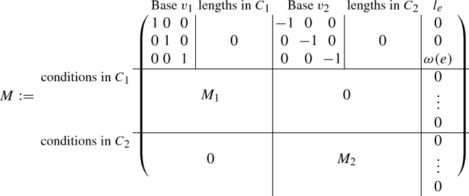
  is a square matrix. Subtract the first three rows of M from the rows of $M_1$ in M to obtain a matrix of the form

  

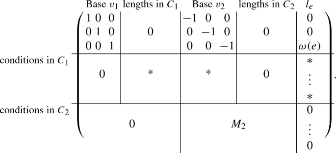
  Notice that there is a $3\times 3$ block matrix in the upper left and that its associated other block in the lower right is precisely the ${\text {ev}}$-matrix of C with base point $v_2$. Therefore

  $$\begin{aligned} {\text {mult}}(C)=|\det (M)|. \end{aligned}$$

  (10)

  On the other hand, general Laplace expansion with respect to the first three rows of M can be used to determine $|\det (M)|$: Denote the number of rows (resp. columns) of M by t and let $M(a_1,\dots ,a_r\mid b_1,\dots b_r)$ denote the $r\times r$ minor of M that is given by the columns $a_1,\dots ,a_r$ and rows $b_1,\dots ,b_r$ of M. Then

  $$\begin{aligned} |\det (M)| =&| \sum _{1\le k_1< k_2 < k_3 \le t} \epsilon (k_1,k_2,k_3)\cdot M(k_1,k_2,k_3\mid 1,2,3)\nonumber \\&\cdot M(l_1,\dots , l_{t-3}\mid 4, \dots , t)|, \end{aligned}$$

  (11)

  where $\lbrace l_1,\dots , l_{t-3}\rbrace \cup \lbrace k_1,k_2,k_3 \rbrace =[t]$ and

  $$\begin{aligned} \epsilon (k_1,k_2,k_3):={\text {sgn}}\left( \begin{array}{cccccc} 1&{} 2&{} 3 &{} 4 &{} \dots &{} t \\ k_1&{} k_2 &{} k_3&{} j_1 &{} \dots &{} j_{t-3} \end{array}\right) , \end{aligned}$$

  where $j_1<\dots < j_{t-3}$ such that $\lbrace k_1,k_2,k_3 \rbrace \cup \lbrace j_1,\dots ,j_{t-3}\rbrace = [t]$. Notice that in (11) a summand can only be nonzero if each $k_i$ does not correspond to a zero-column in the first three rows of M. Moreover, $k_3=t$ must be satisfied since otherwise $M(l_1,\dots , l_{t-3}\mid 4, \dots , t)$ is zero due to a zero-column (the $l_e$-column). Hence

  $$\begin{aligned} |\det (M)| =&| \sum _{1\le k_1< k_2 < t} \epsilon (k_1,k_2,t)\cdot M(k_1,k_2,t\mid 1,2,3) \nonumber \\&\quad \cdot M(l_1,\dots , l_{t-3}\mid 4, \dots , t)|, \end{aligned}$$

  (12)

  where $k_1,k_2$ are columns associated to the base point $v_1$ or $v_2$. Therefore (12) breaks down to four summands. Let $M_{i,{\hat{j}}}$ denote the matrix $M_i$ without its j-th column. The four relevant summands of (12) are

  

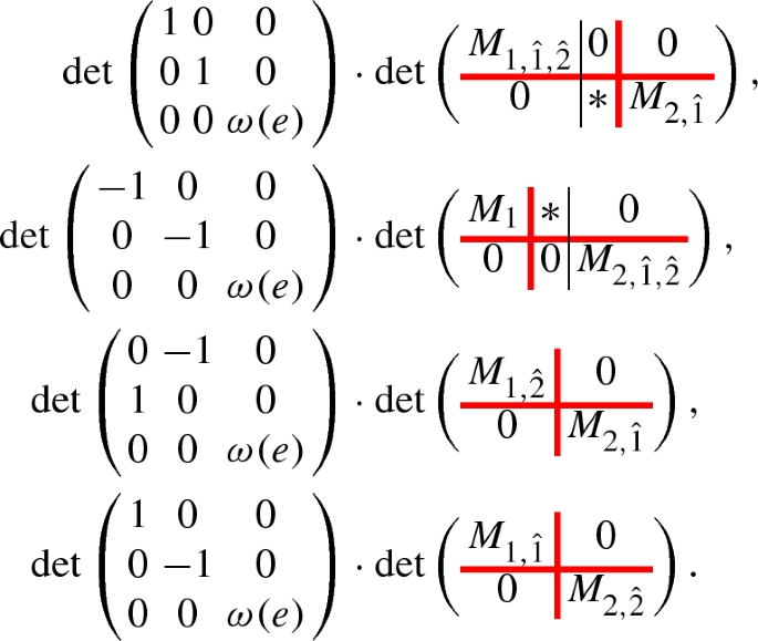
  The bold red lines indicate square boxes in the matrices. Notice that the first two listed summands vanish. Using Notation 2.18 yields that

  

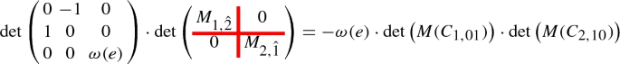
  and

  

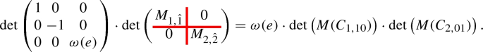
  The signs $\epsilon (k_1,k_2,k_3)$ appearing in (12) are all the same as one can see from a case-by-case analysis distinguishing if the numbers of columns of $M_1$ (resp. $M_2$) are even or odd. Thus (12) yields

  $$\begin{aligned} |\det (M)|=&\omega (e)\cdot | \det \left( M(C_{1,10})\right) \cdot \det \left( M(C_{2,01})\right) \\&- \det \left( M(C_{1,01})\right) \cdot \det \left( M(C_{2,10})\right) |. \end{aligned}$$

  The desired equation now follows from (10).

$\square$

4 Cross-ratio floor diagrams

In this section, cross-ratio floor diagrams are defined. The basic idea is to use floor graphs and equip them with additional data which reflects which conditions are satisfied at which floors that degenerate to a vertex of a floor graph.

Definition 3.1

(Cross-ratio floor diagram) Let $p_{[n]},L_{{\underline{\kappa }}^\alpha },L_{{\underline{\kappa }}^\beta },P_{{\underline{\eta }}^\alpha },P_{{\underline{\eta }}^\beta },\lambda _{[l]}$ be general positioned conditions as in Definition 1.22 with respect to the degree $\Delta ^3_d(\alpha ,\beta )$, i.e.

$$\begin{aligned} \#\Delta ^3_d(\alpha ,\beta )=2n+l+2\cdot \#\left( {\underline{\eta }}^\alpha \cup {\underline{\eta }}^\beta \right) +\#\left( {\underline{\kappa }}^\alpha \cup {\underline{\kappa }}^\beta \right) . \end{aligned}$$

Moreover, each entry of a degenerated tropical cross-ratio is a label of a contracted end or a label of an end of primitive direction $(0,0,\pm 1)\in {\mathbb {R}}^3$.

A cross-ratio floor diagram ${\mathcal {F}}$ (that satisfies the given conditions) is a tree without ends on a totally ordered set of vertices $v_1<\dots <v_n$ with a flow structure that is a condition flow of type 3 such that ${\mathcal {F}}$ satisfies the following properties:

• (1) Each vertex is labeled with a possibly empty set of labeled ends $\delta _{v_i}\subset \Delta ^3_d(\alpha ,\beta )$ such that $\delta _{v_i}\cap \delta _{v_j}=\varnothing$ for all $i\ne j$ and $\bigcup _{i=1}^n \delta _{v_i}=\Delta ^3_d(\alpha ,\beta )$.

• (2) Each edge e of ${\mathcal {F}}$ (consisting of two half-edges) is equipped with a weight $\omega (e)\in {\mathbb {N}}_{>0}$ such that vertices $v_i$ of ${\mathcal {F}}$ are balanced with respect to these weights, i.e.

  $$\begin{aligned} \#\delta _{v_i}^{(1,1,1)}+\sum _{e'\in \delta _{v_i}^\beta }\omega (e')+\sum _{\begin{array}{c} e \text {an edge}\\ \text {between } v_i<v_j \end{array}} \omega (e) -\sum _{e'\in \delta _{v_i}^\alpha }\omega (e')- \sum _{\begin{array}{c} e \text { an edge}\\ \text {between } v_j<v_i \end{array}} \omega (e)=0 \end{aligned}$$

  holds for all $i\in [n]$, where $\delta _{v_i}^{(1,1,1)}$ is the subset of $\delta _{v_i}$ that contains all ends of primitive direction (1, 1, 1), $\delta _{v_i}^\beta$ is the subset of $\delta _{v_i}$ that contains all ends of primitive direction (0, 0, 1) and $\delta _{v_i}^\alpha$ is the subset of $\delta _{v_i}$ that contains all ends of direction $(0,0,-1)$.

• (3) The graph ${\mathcal {F}}$ satisfies the given degenerated tropical cross-ratios $\lambda _{[n]}$. More precisely, ${\mathcal {F}}$ satisfies a degenerated tropical cross-ratio $\lambda _j$ if ${\mathcal {F}}$ satisfies the path criterion (see Remark 1.31) for $j\in [l]$, where the paths’ end points are given as follows. If $\beta _t$ is an entry of $\lambda _j$ that is the label of a contracted end $x_i$ that satisfies a point condition $p_i$, then the end point associated to $\beta _t$ is the vertex $v_i$. If $\beta _t$ is the label of a non-contracted end instead, i.e. this end appears in $\delta _{v_i}^\alpha$ or $\delta _{v_i}^\beta$ for some vertex $v_i$, then the end point associated to $\beta _t$ is $v_i$. We say that the degenerated tropical cross-ratio $\lambda _j$ is satisfied at a vertex $v_i$ of ${\mathcal {F}}$ if the paths associated to $\lambda _j$ intersect only in $v_i$. The set of all tropical cross-ratios satisfied at a vertex $v_i$ is denoted by $\lambda _{v_i}$ and $\#\lambda _{v_i}\in {\mathbb {N}}$ is called the number of tropical cross-ratios at $v_i$.

• (4) For every vertex $v_i$ of ${\mathcal {F}}$, let $\delta _{v_i}^{\alpha },\delta _{v_i}^{\beta },\delta _{v_i}^{\alpha ,P},\delta _{v_i}^{\beta , P},\delta _{v_i}^{\alpha ,L},\delta _{v_i}^{\beta ,L}$ denote the submultisets of all labeled ends $\delta _{v_i}$ associated to $v_i$ such that

  • $\delta _{v_i}^{\alpha }$ (resp. $\delta _{v_i}^{\beta }$) are the ends that are associated to $\alpha$ (resp. $\beta$),

  • $\delta _{v_i}^{\alpha ,P}\subset \delta _{v_i}^{\alpha }$ (resp. $\delta _{v_i}^{\beta ,P}\subset \delta _{v_i}^{\beta }$) are the ends that satisfy some codimension one tangency conditions (see Notation 1.23),

  • $\delta _{v_i}^{\alpha ,L}\subset \delta _{v_i}^{\alpha }$ (resp. $\delta _{v_i}^{\beta ,L}\subset \delta _{v_i}^{\beta }$) are the ends that satisfy some codimension two tangency conditions (see Notation 1.23).

  Let ${\text {val}}(v_i)$ denote the valence of $v_i$ in ${\mathcal {F}}$. Define

  $$\begin{aligned} A(v_i)&:=3\cdot \#\delta _{v_i}^{(1,1,1)}+ \#\delta _{v_i}^{\alpha }+ \#\delta _{v_i}^{\beta }+{\text {val}}(v_i) -2 -\#\lambda _{v_i}-2( \#\delta _{v_i}^{\alpha ,P}\\&\qquad + \#\delta _{v_i}^{\beta , P})- \#\delta _{v_i}^{\alpha ,L}- \#\delta _{v_i}^{\beta ,L}. \end{aligned}$$

  The flow of the vertex $v_i$ of ${\mathcal {F}}$ is given by

  $$\begin{aligned} {\text {flow}}(v_i)= \left\{ \begin{array}{ll} 0 &{}\text {, if } \delta _{v_i}^{(1,1,1)}=\varnothing \\ A(v_i) &{}\text {, else}\\ \end{array}\right. \end{aligned}$$

  Notice that this flows determine the condition flow of type 3 on ${\mathcal {F}}$ uniquely by Lemma 2.2.

Example 3.2

Let $\Delta ^3_4\left( (4,1,0,\dots ), (2,0,\dots ) \right)$ denote a degree as in Notation 1.9 whose labeling is:

$$\begin{aligned} \begin{array}{c|c|c|c|c|c} \text {Ends of primitive direction}\dots &{} e_3 &{} -e_3 &{} -e_1 &{} -e_2 &{} e_0 \\ \hline \text {its associated labels} &{} 3,9 &{} 4,5,6,7,8 &{} 10,11,12,19 &{} 13,14,15,20 &{} 16,17,18,21 \end{array}, \end{aligned}$$

such that the end of weight two is labeled by 8. Let $p_{[2]}, P_{[9]\backslash [2]}, \lambda _1=\lbrace 1,2,3,7 \rbrace$ general positioned conditions with notation from Definition 1.22. Recall the floor graph from Example 2.13. Equipping it with discrete data as below turns it into a cross-ratio floor diagram ${\mathcal {F}}$ that satisfies $p_{[2]}, P_{[9]\backslash [2]}, \lambda _1$.

i	1	2
$\delta _{v_i}$	$[18]\backslash \lbrace 2,9 \rbrace$	$\lbrace 2,9,19,20,21\rbrace$
$\delta _{v_i}^{(1,1,1)}$	$\lbrace 16,17,18\rbrace$	$\lbrace 21\rbrace$
$\delta _{v_i}^\alpha$	$\lbrace 4,5,6,7,8 \rbrace$	$\varnothing$
$\delta _{v_i}^\beta$	$\lbrace 3 \rbrace$	$\lbrace 9 \rbrace$
$\lambda _{v_i}$	$\lbrace \lambda _1 \rbrace$	$\varnothing$
$\delta _{v_i}^{\alpha ,P}$	$\lbrace 4,5,6,7,8 \rbrace$	$\varnothing$
$\delta _{v_i}^{\beta ,P}$	$\lbrace 3 \rbrace$	$\lbrace 9 \rbrace$
$\delta _{v_i}^{\alpha ,L}$	$\varnothing$	$\varnothing$
$\delta _{v_i}^{\beta ,L}$	$\varnothing$	$\varnothing$

Definition 3.3

(Multiplicity of a cross-ratio floor diagram) Let $p_{[n]},L_{{\underline{\kappa }}^\alpha },L_{{\underline{\kappa }}^\beta },P_{{\underline{\eta }}^\alpha },P_{{\underline{\eta }}^\beta },\lambda _{[l]}$ be general positioned conditions and let ${\mathcal {F}}$ be a cross-ratio floor diagram as in Definition 3.1 that satisfies the given conditions. Let $v_1<\cdots <v_n$ denote the totally ordered vertices of ${\mathcal {F}}$. For $\gamma =\alpha ,\beta$, define the following: Let $\underline{{2/0}_i}^\gamma$ be the 2/0 edges adjacent to $v_i$ and $v_j$ (with $j\ne i$) in ${\mathcal {F}}$ such that $j<i$ if $\gamma =\alpha$ and $i<j$ if $\gamma =\beta$. Let $\underline{{1/1}_i}^\gamma$ be the 1/1 edges adjacent to $v_i$, where $\gamma \in \lbrace \alpha ,\beta \rbrace$ is defined analogously.

For a vertex $v_i$ of the cross-ratio floor diagram ${\mathcal {F}}$, its multiplicity ${\text {mult}}(v_i)$ is defined as

$$\begin{aligned} {\text {mult}}(v_i):=N_{\Delta ^3_{\#\delta _{v_i}^{(1,1,1)}}\left( \alpha ^{i},\beta ^{i} \right) }\left( p_i, L_{\delta _{v_i}^{\alpha ,L} \cup \underline{{1/1}_i}^\alpha },L_{\delta _{v_i}^{\beta ,L} \cup \underline{{1/1}_i}^\beta },P_{\delta _{v_i}^{\alpha ,P} \cup \underline{{2/0}_i}^\alpha },P_{\delta _{v_i}^{\beta ,P} \cup \underline{{2/0}_i}^\beta },\lambda ^{\rightarrow }_{v_i} \right) , \end{aligned}$$

with notation from 3.1 and Notation 1.1, where $\alpha ^{i}$ (resp. $\beta ^{i}$) of the degree $\Delta ^3_{\#\delta _{v_i}^{(1,1,1)}}\left( \alpha ^{i},\beta ^{i} \right)$ arises from $\delta _{v_i}^\alpha$ (resp. $\delta _{v_i}^\beta$) and edges contributing to ${\text {val}}(v_i)$ in ${\mathcal {F}}$, and where $L_{\underline{{1/1}_i}^\alpha }$ (resp. $L_{\underline{{1/1}_i}^\beta }$) are collections of tropical multi-line conditions with ends of weight 1. Moreover, the cross-ratios $\lambda _{v_i}$ are adapted to cutting the edges adjcent to $v_i$ similar to Construction 2.10. The multiplicity of the entire cross-ratio floor diagram ${\mathcal {F}}$ is defined to be the product of the vertices’ multiplicities times the edges’ weights, i.e.

$$\begin{aligned} {\text {mult}}({\mathcal {F}}):=\prod _{\begin{array}{c} e \text { edge}\\ \text { of } {\mathcal {F}} \end{array}} \omega (e)\cdot \prod _{i=1}^n {\text {mult}}(v_i). \end{aligned}$$

Example 3.4

Let ${\mathcal {F}}$ be the cross-ratio floor diagram of Example 3.2. Label its edge of weight two by 22. The multiplicities of the vertices $v_1,v_2$ of ${\mathcal {F}}$ are

$$\begin{aligned} {\text {mult}}(v_1)&=N_{\Delta ^3_{3}\left( (4,1,0,\dots ),(1,1,0,\dots ) \right) }\left( p_1,L_{22},P_{[8]\backslash [2]}, \lambda _1^{\rightarrow 22} \right) ,\\ {\text {mult}}(v_2)&=N_{\Delta ^3_{1}\left( (0,1,0,\dots ),(1,0,\dots ) \right) }\left( p_2,L_{22},P_{9} \right) , \end{aligned}$$

where $\lambda _1^{\rightarrow 22}=\lbrace 1,22,3,7\rbrace$ and $L_{22}$ is a tropical multi-line with ends of weight 1 (we use Notation 1.23).

Definition 3.5

Given a set of general positioned conditions $p_{[n]},L_{{\underline{\kappa }}^\alpha },L_{{\underline{\kappa }}^\beta },P_{{\underline{\eta }}^\alpha },P_{{\underline{\eta }}^\beta },\lambda _{[l]}$ as in Definition 3.1 with respect to the degree $\Delta ^3_d(\alpha ,\beta )$, the number of cross-ratio floor diagrams satisfying these conditions is defined by

$$\begin{aligned} N^{{\text {floor}}}_{\Delta ^3_d(\alpha ,\beta )}\left( p_{[n]},L_{{\underline{\kappa }}^\alpha },L_{{\underline{\kappa }}^\beta },P_{{\underline{\eta }}^\alpha },P_{{\underline{\eta }}^\beta },\lambda _{[l]}\right) := \sum _{{\mathcal {F}}} {\text {mult}}({\mathcal {F}}), \end{aligned}$$

where the sum goes over all cross-ratio floor diagrams that satisfy the given conditions.

4.1 Multiplicity of a cross-ratio floor diagram via curves in ${\mathbb {R}}^2$

The following proposition reduces the calculation of the multiplicity of a cross-ratio floor diagram to the enumeration of rational tropical stable maps to ${\mathbb {R}}^2$ satisfying point, multi-line and cross-ratio conditions.

Proposition 3.6

For notation, see Notation 1.1, 1.11 and Definition 3.3. The multiplicity ${\text {mult}}(v_i)$ of a vertex $v_{i}$ of a cross-ratio floor diagram that satisfies general positioned conditions equals the degree of the cycle

$$\begin{aligned} \begin{aligned}&\prod _{k\in \underline{\kappa _{i}}^{\alpha }\cup \underline{\kappa _{i}}^{\beta }} {\text {ev}}_k^{*}(L_k) \cdot \prod _{f\in \underline{\eta _{i}}^{\alpha }\cup \underline{\eta _{i}}^{\beta }} {\text {ev}}_f^{*}(P_f) \cdot \prod _{\lambda _j\in \lambda _{v_i}} {\text {ft}}_{\lambda ^{\rightarrow }_j}^*\left( 0\right) \cdot {\text {ev}}_i^*\left( \pi (p_i)\right) \\&\quad \cdot {\mathcal {M}}_{0,1+|\alpha ^{i}|+|\beta ^{i}|}\left( {\mathbb {R}}^2,\pi \left( \Delta ^3_{\#\delta _{v_i}^{(1,1,1)}}\left( \alpha ^{i},\beta ^{i} \right) \right) \right) , \end{aligned} \end{aligned}$$

(13)

where $\underline{\kappa _{i}}^{\gamma }:=\delta _{v_i}^{\gamma ,L} \cup \underline{{1/1}_i}^\gamma$ and $\underline{\eta _{i}}^{\gamma }:=\delta _{v_i}^{\gamma ,P} \cup \underline{{2/0}_i}^\gamma$ for $\gamma =\alpha ,\beta$.

Proof

Notice that since the given conditions $p_i, L_{\underline{\kappa _{i}}^{\alpha }},L_{\underline{\kappa _{i}}^{\beta }},P_{\underline{\eta _{i}}^{\alpha }},P_{\underline{\eta _{i}}^{\beta }},\lambda ^{\rightarrow }_{v_i}$ are in general position with respect to $\Delta ^3_{\#\delta _{v_i}^{(1,1,1)}}\left( \alpha ^{i},\beta ^{i} \right)$ and there is only one point condition $p_i$, we can assume that the conditions $\pi (p_i), L_{\underline{\kappa _{i}}^{\alpha }},L_{\underline{\kappa _{i}}^{\beta }},P_{\underline{\eta _{i}}^{\alpha }},P_{\underline{\eta _{i}}^{\beta }},\lambda ^{\rightarrow }_{v_i}$ are also in general position with respect to the degree $\pi \left( \Delta ^3_{\#\delta _{v_i}^{(1,1,1)}}\left( \alpha ^{i},\beta ^{i} \right) \right)$. Using (3), we see that the cycle (13) is indeed 0-dimensional. Thus considering its degree makes sense.

Let C be a tropical stable map contributing to ${\text {mult}}(v_i)$. Applying the map ${\tilde{\pi }}$ from Notation 1.11 induced by the projection $\pi :{\mathbb {R}}^3\rightarrow {\mathbb {R}}^2$ that forgets the z-coordinate leads to a tropical stable map ${\tilde{\pi }}(C)$ that contributes to (13). Vice versa, a tropical stable map $C'$ that contributes to (13) can be lifted uniquely to a tropical stable map C that contributes to ${\text {mult}}(v_i)$, because the z-coordinates of the directions of the edges can be recovered from the balancing condition and the overall z-position of C is fixed by the z-coordinate of $p_i$. Hence $\pi$ induces a bijection between tropical stable maps C that contribute to ${\text {mult}}(v_i)$ and tropical stable maps ${\tilde{\pi }}(C)$ that contribute to (13).

It remains to show that the multiplicities of C and ${\tilde{\pi }}(C)$ coincide. For that notice that the cross-ratio multiplicities of every vertex $v\in C$ and its image $\pi (v_i)$ in ${\tilde{\pi }}(C)$ coincide. Thus it remains to show that the ${\text {ev}}$-multiplicities coincide as well. The ${\text {ev}}$-multiplicity of C (resp. ${\tilde{\pi }}(C)$) is given by the absolute value of the determinant of the ${\text {ev}}$-Matrix M(C) (resp. the ${\text {ev}}$-matrix $M({\tilde{\pi }}(C))$) associated to C (resp. ${\tilde{\pi }}(C)$), see Definition 1.35. We choose $p_i$ as base point for the local coordinates used for M(C) (resp. $\pi (p_i)$ as base point for $M({\tilde{\pi }}(C))$) which are the lengths of the edges of C (resp. ${\tilde{\pi }}(C)$). The matrix $M({\tilde{\pi }}(C))$ is obtained from M(C) by erasing the third column and row which intersect in the z-coordinate of the base point, which is 1 (see below). The matrices M(C) and $M({\tilde{\pi }}(C))$ look like follows

Recall that $\partial {\text {ev}}$ is by definition ${\text {ev}}\circ \pi$, i.e. the submatrices B, M marked above are equal. Therefore

$$\begin{aligned} |\det (M(C))|=|\det (M({\tilde{\pi }}(C))| \end{aligned}$$

follows from using Laplace expansion on the third row of M(C). $\square$

There is a general Kontsevich’s formula [15] which recursively calculates the weighted number of rational tropical curves in ${\mathbb {R}}^2$ that satisfy point, multi-line and cross-ratio conditions. As a consequence, the multiplicity of a cross-ratio floor diagram can be determined recursively.

Corollary 3.7

The multiplicity ${\text {mult}}(v_i)$ of a vertex $v_{i}$ of a cross-ratio floor diagram can be calculated recursively using the general Kontsevich’s formula from [15].

Example 3.8

Let ${\mathcal {F}}$ be the cross-ratio floor diagram of Example 3.2. Using Proposition 3.6 to express ${\text {mult}}(v_1),{\text {mult}}(v_2)$ of Example 3.4 yields

$$\begin{aligned} {\text {mult}}(v_1)&=N_{\Delta ^2_{3}}\left( \pi (p_1),\pi \left( P_{[8]\backslash [2]}\right) , L_{22} \lambda _1^{\rightarrow 22} \right) ,\\ {\text {mult}}(v_2)&=N_{\Delta ^2_{1}}\left( \pi (p_2),\pi \left( P_{9}\right) , L_{22} \right) . \end{aligned}$$

This allows us to use Corollary 3.7, resp. general Kontsevich’s formula [15]. Hence

$$\begin{aligned} {\text {mult}}(v_1)&=5,\\ {\text {mult}}(v_2)&=1. \end{aligned}$$

Therefore ${\text {mult}}({\mathcal {F}})=10$.

5 Counting tropical curves using cross-ratio floor diagrams

The aim of this section is to prove the following theorem which is the main result of this paper. It reduces the count of spatial curves satisfying given conditions to a counting problem of cross-ratio floor diagrams. There are only finitely many cross-ratio floor diagrams to given conditions. Thus the weighted number of cross-ratio floor diagrams satisfying given conditions can be determined by going through all possible cross-ratio floor diagrams, which then answers the initial counting problem.

Theorem 4.1

For notations, see Definition 1.22, 1.27 and Notation 1.1, 1.9. Consider general positioned conditions $p_{[n]},L_{{\underline{\kappa }}^\alpha },L_{{\underline{\kappa }}^\beta },P_{{\underline{\eta }}^\alpha },P_{{\underline{\eta }}^\beta },\lambda _{[l]}$ with respect to a degree $\Delta _d^3(\alpha ,\beta )$ such that each entry of a degenerated tropical cross-ratio is a label of a contracted end or a label of an end of primitive direction $(0,0,\pm 1)\in {\mathbb {R}}^3$. Then

$$\begin{aligned}&N^{{\text {floor}}}_{\Delta ^3_d(\alpha ,\beta )}\left( p_{[n]},L_{{\underline{\kappa }}^\alpha },L_{{\underline{\kappa }}^\beta },P_{{\underline{\eta }}^\alpha },P_{{\underline{\eta }}^\beta },\lambda _{[l]}\right) \nonumber \\&\quad = N_{\Delta ^3_d(\alpha ,\beta )}\left( p_{[n]},L_{{\underline{\kappa }}^\alpha },L_{{\underline{\kappa }}^\beta },P_{{\underline{\eta }}^\alpha },P_{{\underline{\eta }}^\beta },\lambda _{[l]}\right) \end{aligned}$$

(14)

holds, i.e. the weighted count of cross-ratio floor diagrams satisfying the given conditions equals the weighted count of rational tropical stable degree $\Delta _d^3(\alpha ,\beta )$ maps to ${\mathbb {R}}^3$ satisfying the given conditions.

Construction 4.2

(Floor decomposed tropical stable map $\mapsto$ cross-ratio floor diagram) Let C be a floor decomposed tropical stable map contributing to $N_{\Delta _d^3(\alpha ,\beta )}\left( p_{[n]},L_{{\underline{\kappa }}^\alpha },L_{{\underline{\kappa }}^\beta },P_{{\underline{\eta }}^\alpha },P_{{\underline{\eta }}^\beta },\lambda _{[l]} \right)$. We want to construct a cross-ratio floor diagram ${\mathcal {F}}$ as in Definition 3.1 (that satisfies given conditions) with vertices $v_1<\cdots <v_n$.

Let ${\mathcal {F}}$ denote the floor graph associated to C, see Definition 2.8. To make sure that ${\mathcal {F}}$ is indeed a cross-ratio floor diagram, properties (1), (2), (3) and (4) of Definition 3.1 must be satisfied. For (1), define $\delta _{v_i}$ as the multiset of ends adjacent to the floor $C_i$ of C which satisfies the point condition $p_i$. Property (2) follows from balancing of C. For (3), define $\lambda _{v_i}$ as the union over all $\lambda _{u_j}$ (the set of cross-ratios satisfied at $u_j$), where $u_j$ is a vertex of the floor $C_i$, and use the path criterion (Remark 1.31) to verify that ${\mathcal {F}}$ satisfies the cross-ratios $\lambda _{[l]}$ if C does. Property (4) is more technical: If the floor $C_i$ does not contain an end of direction (1, 1, 1) (i.e. if $\delta _{v_i}^{(1,1,1)}=\varnothing$ with the notation from Definition 3.1), then ${\text {flow}}(v_i)=0$ since $C_i$ consists of a single vertex satisfying the point condition $p_i$.

Let now $\delta _{v_i}^{(1,1,1)}\ne \varnothing$. Cutting all elevators adjacent to the floor $C_i$ of C as in Construction 2.10 yields general positioned conditions $p_i,L_{\underline{\kappa _i}^\alpha },L_{\underline{\kappa _i}^\beta },P_{\underline{\eta _i}^\alpha },P_{\underline{\eta _i}^\beta },\lambda _{\underline{l_i}}^{\rightarrow }$ it satisfies. Hence (1) gives us

$$\begin{aligned} \#\Delta ^3_{s_i}\left( \alpha ^{i},\beta ^{i} \right) = 2+2\cdot \#\left( \underline{\eta _i}^\alpha \cup \underline{\eta _i}^\beta \right) + \#\left( \underline{\kappa _i}^\alpha \cup \underline{\kappa _i}^\beta \right) + \#\underline{l_i}. \end{aligned}$$

(15)

By definition, we have

$$\begin{aligned} \begin{aligned} \#\underline{l_i}&= \#\lambda _{v_i},\\ \#\Delta ^3_{s_i}\left( \alpha ^{i},\beta ^{i} \right)&= 3\cdot \#\delta _{v_i}^{(1,1,1)}+ \#\delta _{v_i}^{\alpha }+ \#\delta _{v_i}^{\beta }+{\text {val}}(v_i).\\ \end{aligned} \end{aligned}$$

(16)

Moreover,

$$\begin{aligned} 2\cdot \#\left( \underline{\eta _i}^\alpha \cup \underline{\eta _i}^\beta \right) + \#\left( \underline{\kappa _i}^\alpha \cup \underline{\kappa _i}^\beta \right) =&2\cdot \left( \#\delta _{v_i}^{\alpha ,P} + \#\delta _{v_i}^{\beta , P} \right) \nonumber \\&+ \#\delta _{v_i}^{\alpha ,L}+ \#\delta _{v_i}^{\beta ,L} + {\text {flow}}(v_i) \end{aligned}$$

(17)

holds, where ${\text {flow}}(v_i)$ comes from the conditions imposed on $C_i$ via elevators and the rest comes from given tangency conditions that ends adjacent to $C_i$ satisfy. Property (4) follows from applying (16) and (17) to (15) and resolving for ${\text {flow}}(v_i)$. Notice that the conditions flow associated to ${\mathcal {F}}$ this way coincides with the one of Definition 2.12.

Example 4.3

Let ${\mathcal {F}}$ be the cross-ratio floor diagram of Example 3.2. Observe that the floor decomposed tropical stable map C of Example 2.6 degenerates to ${\mathcal {F}}$ if the labels of ends that are not shown in Fig. 4 are chosen appropriately, i.e. to fit Example 3.2.

Figure 8 shows another floor decomposed tropical stable map D. It satisfies the degenerated tropical cross-ratio $\lambda _1=\lbrace 1,2,3,7\rbrace$. Moreover, we claim that it is possible to assign lengths to the bounded edges of D in its schematic representation in Fig. 8 in such a way that D satisfies the same conditions as C. The conditions in question are point conditions $p_1,p_2$ and the codimension one tangency conditions $P_{[9]\backslash [2]}$. Cut the elevators of C and D, project the floors to ${\mathbb {R}}^2$ using $\pi$ as in the proof of Proposition 3.6. Notice that it is sufficient to check whether the projections of the floors $C_1$ and $D_1$ satisfy the same conditions. For that, use the cross-ratio lattice path algorithm from [16] with the degenerated cross-ratio $\lambda _1$ to obtain the projections $\pi (C_1)$ and $\pi (D_1)$ that then satisfy $\pi \left( p_{[2]}\right)$ and $\pi \left( P_{[9]\backslash [2]}\right)$. Lifting $\pi (C_1)$ and $\pi (D_1)$ yields the desired lengths. The lattice path calculation can be found in Example 3.15, Figure 9 of [16]. More precisely, $\pi (C_1)$ corresponds to the entry (read as a matrix) (6, 2), and $\pi (D_1)$ corresponds to the entry (4, 2) of Figure 9 loc. cit..

Thus D degenerates to ${\mathcal {F}}$ as well if the missing labels in Fig. 8 are chosen appropriately.

Fig. 8

The tropical stable map D from Example 4.3 which is floor decomposed. It has two floors $D_i$ for $i=1,2$. The dashed edge is the elevator of weight two of D

Proof of Theorem 4.1

Since the numbers in question are independent of the exact positions of the given conditions, we can assume that all given conditions are in stretched configuration (see Definition 2.3). Thus (by Proposition 2.7) every tropical stable map contributing to the right-hand side of (14) is floor decomposed. Hence Construction 4.2 associates a cross-ratio floor diagram to every tropical stable map contributing to the right-hand side of (14). Therefore it is sufficient to show for a fixed cross-ratio floor diagram ${\mathcal {F}}$ (that satisfies the given conditions) that

$$\begin{aligned} {\text {mult}}({\mathcal {F}})=\sum _{C \rightarrow {\mathcal {F}}} {\text {mult}}(C) \end{aligned}$$

(18)

holds (where the sum goes over all C degenerating to ${\mathcal {F}}$), i.e. that the multiplicity with which a cross-ratio floor diagram ${\mathcal {F}}$ is counted equals the sum of the multiplicities of all tropical stable maps C contributing to the right-hand side of (14) such that C degenerates to ${\mathcal {F}}$. So fix a cross-ratio floor diagram ${\mathcal {F}}$.

To shorten notation, let $B:=\lbrace p_{[n]},L_{{\underline{\kappa }}^\alpha },L_{{\underline{\kappa }}^\beta },P_{{\underline{\eta }}^\alpha },P_{{\underline{\eta }}^\beta },\lambda _{[l]} \rbrace$ be the set of conditions that ${\mathcal {F}}$ satisfies, and let $N^{{\text {floor}}}(B)$ (resp. N(B)) denote the number on the left-hand side (resp. the right-hand side) of (14). Assume that ${\mathcal {F}}$ has more than 1 vertex, because otherwise there is nothing to show. Since ${\mathcal {F}}$ is a tree, there is a 1-valent vertex $v_i$ of ${\mathcal {F}}$ adjcacent to a vertex $v_j$ with $i<j$ via an edge q. There are two cases: q is either a 1/1 edge or a 2/0 edge. First, assume that q is a 1/1 edge. Let $L^{(j)}$ (resp. $L^{(i)}$) be the codimension two condition from Corollary 2.15 which $v_i$ passes to $v_j$ via q (resp. $v_j$ passes to $v_i$). Notice that the conditions $L^{(j)}$ (resp. $L^{(i)}$) are cycles in ${\mathbb {R}}^2$ as in Proposition 2.14. Those cycles depend only on the given conditions and the cross-ratio floor diagram ${\mathcal {F}}$ contains the information about how the conditions are distributed to the floors of each tropical stable maps that degenerates to ${\mathcal {F}}$. Hence $L^{(j)}$ (resp. $L^{(i)}$) do only depend on the cross-ratio floor diagram ${\mathcal {F}}$.

We follow the idea of recursively moving conditions in such a way that ${\text {mult}}(C)$ can be calculated as a product in which each factor is associated to a floor. Cut q to obtain two new cross-ratio floor diagrams ${\mathcal {F}}_i$ and ${\mathcal {F}}_j$, where ${\mathcal {F}}_i$ consists of a single vertex $v_i$ and ${\mathcal {F}}_j$ is given by ${\mathcal {F}}$ without $v_i$. Decomposing ${\mathcal {F}}$ into ${\mathcal {F}}_i$ and ${\mathcal {F}}_j$ decomposes B into $B_i$ and $B_j$ as well, more precisely, let $B_i\subset B$ (resp. $B_j\subset B$) be the subset of conditions ${\mathcal {F}}_i\subset {\mathcal {F}}$ (resp. ${\mathcal {F}}_j$) satisfies. Notice that the set of all conditions ${\mathcal {F}}_i$ (resp. ${\mathcal {F}}_j$) satisfies is $B_i\cup L^{(i)}$ (resp. $B_j\cup L^{(j)}$).

If we change the x- and y-coordinates of the conditions in $B_i$ and $B_j$ in such a way that all conditions are still in a stretched configuration, then any tropical stable map C with $C\rightarrow {\mathcal {F}}$ is still floor decomposed and still degenerates to ${\mathcal {F}}$. More precisely, we are allowed to move the x- and y-coordinates of the conditions in $B_i$ and $B_j$ inside a box, which is small compared to the stretching of the conditions in z-direction. Notice that moving conditions as above moves $L^{(i)}$ and $L^{(j)}$ accordingly. Hence we can achieve (by bringing the x, y-positions of conditions in $B_{j}$ (resp. $B_{i}$) arbitrarily close together) that $L^{(i)}$ and $L^{(j)}$ intersect in the following way: all points of the intersection of $L^{(i)}$ and $L^{(j)}$ are on the ends of $L^{(i)}$ that are of primitive direction $(0,-1)\in {\mathbb {R}}^2$, and on the ends of $L^{(j)}$ that are of primitive direction $(-1,0)\in {\mathbb {R}}^2$, see Fig. 9. Thus, using part (b) of Lemma 2.20 (where the second summand vanishes) and Notation 2.18, we have

$$\begin{aligned} \sum _{C \rightarrow {\mathcal {F}}} {\text {mult}}(C) = \omega (q) \sum _{C \rightarrow {\mathcal {F}}} {\text {mult}}\left( C_{i,10}\right) \cdot {\text {mult}}\left( C_{j,01}\right) \end{aligned}$$

where $\omega (q)$ is the weight of our cut edge q and $C_i,C_j$ are the pieces obtained from C by cutting e.

Fig. 9

Codimension two tangency conditions $L^{(i)}$ and $L^{(j)}$ after movement, together with the codimension two tangency conditions $E^{(i)}$ and $E^{(j)}$, where $p\in L^{(i)}\cap L^{(j)}$ is the point associated to $\pi (V_i)$ and $\pi (V_j)$

We claim that

$$\begin{aligned} \sum _{C \rightarrow {\mathcal {F}}} {\text {mult}}\left( C_{i,10}\right) \cdot {\text {mult}}\left( C_{j,01}\right) = N(B_i\cup \lbrace E^{(i)} \rbrace )\cdot \sum _{C_j \rightarrow {\mathcal {F}}_j} {\text {mult}}(C_j), \end{aligned}$$

(19)

where ${\mathcal {F}}_j$ is understood as a cross-ratio floor diagram that satisfies the conditions $B_j\cup \lbrace E^{(j)} \rbrace$, and where $E^{(i)}$ and $E^{(j)}$ are codimension two tangency conditions that are tropical multi-lines in ${\mathbb {R}}^2$ with ends of weight 1. To see this, let $E^{(i)}$ and $E^{(j)}$ be two tropical lines with ends of weight 1 whose positions are chosen according to Fig. 9, i.e. choose $E^{(i)}$ (resp. $E^{(j)}$) in such a way that it intersects $L^{(j)}$ (resp. $L^{(i)}$) only in its rays of primitive direction $(-1,0)$ (resp. $(0,-1)$) and such that each point of intersection locally looks like the x and y axes’ intersection.

Each tropical stable map $C_i$ contributing to $N(B_i\cup \lbrace E^{(i)} \rbrace )$ has an end q parallel to the z-axis whose adjacent vertex $V_i$ is 3-valent and satisfies $\pi (V_i)\in L^{(j)}\cap E^{(i)}$, where $\pi$ is the projection that forgets the z-coordinate. This is true due to Proposition 2.14 and since $C_i$ satisfies $L^{(j)}$ by definition of $L^{(j)}$. Analogously, by definition of $L^{(i)}$ and Proposition 2.14, each tropical stable map $C_j$ from the right-hand side of (19) has an end q parallel to the z-axis whose adjacent vertex $V_j$ is 3-valent and satisfies $\pi (V_j)\in L^{(i)}\cap E^{(j)}$. Since $V_i$ (resp. $V_j$) is by Proposition 2.14 adjacent to an end of $C_i$ (resp. $C_j$), we can move $V_i$ and $V_j$ as in Fig. 9 to the corresponding point of intersection of $L^{(j)}\cap L^{(i)}$ such that the combinatorials types of $C_i$ and $C_j$ do not change and such that the multiplicities of $C_i$ and $C_j$ understood as tropical stable maps contributing to the right-hand side of (19) do not change. Since we moved $V_i$ and $V_j$ to one point, we can glue $C_i$ and $C_j$ to obtain a tropical stable map C such that $C\rightarrow {\mathcal {F}}$ and the multiplicities of $C_i$ and $C_j$ (understood as tropical stable maps contributing to the right-hand side of (19)) are equal to ${\text {mult}}\left( C_{i,10}\right)$ and ${\text {mult}}\left( C_{j,01}\right)$ by our special choice of the positions of $L^{(i)}$ and $L^{(j)}$. Reversing the process of glueing yields a bijection between factors of the left and factors of the right-hand side of (19).

The multiplicity of the vertex $v_i$ of ${\mathcal {F}}$ equals $N(B_i\cup \lbrace E^{(i)} \rbrace )$ by Definition 3.3. Moreover, if q is a 2/0 edge instead, then part (a) of Lemma 2.20 guarantees that multiplicities split nicely if edges are cut, so in total (19) gives rise to a recursion that eventually yields

$$\begin{aligned} \sum _{C \rightarrow {\mathcal {F}}} {\text {mult}}\left( C_{i,10}\right) \cdot {\text {mult}}\left( C_{j,01}\right) = \prod _{e\ne q} \omega (e) \cdot \prod _{i=1}^n {\text {mult}}(v_i) \end{aligned}$$

since ${\mathcal {F}}$ is a tree. Hence (18) holds.

Notice that $L^{(i)}$ and $L^{(j)}$ depend on the choice of the floor diagram ${\mathcal {F}}$. So we should use the notation $L_{\mathcal {F}}^{(i)}$ and $L_{\mathcal {F}}^{(j)}$ instead. It remains to show that we can bring $L_{\mathcal {F}}^{(i)}$ and $L_{\mathcal {F}}^{(j)}$ in a position as above for each choice of floor diagram ${\mathcal {F}}$ without effecting the overall weighted count of cross-ratio floor diagrams $N^{{\text {floor}}}_{\Delta ^3_d(\alpha ,\beta )}\left( p_{[n]},L_{{\underline{\kappa }}^\alpha },L_{{\underline{\kappa }}^\beta },P_{{\underline{\eta }}^\alpha },P_{{\underline{\eta }}^\beta },\lambda _{[l]}\right)$. Moving conditions as above does not lead to a tropical stable map degenerating to another cross-ratio floor diagram than it initially did, and the cycle obtained by moving conditions (i.e. by relaxing some of the initially given conditions) as above is balanced. Therefore we can assume that $L_{\mathcal {F}}^{(i)}$ and $L_{\mathcal {F}}^{(j)}$ are always in a position as shown in Fig. 9. $\square$

Corollary 4.4

Notation of Theorem 1.29 is used. Let $\mu _{[l]}$ be non-tropical cross-ratios tropicalizing to $\lambda '_{[l]}$ and let $p_{[n]}$ be point conditions such that $p_{[n]},\lambda _{[l]}$, where $\lambda '_j$ degenerates to $\lambda _j$ for $j\in [l]$, are in general position with respect to the degree $\Delta _d^3(\alpha ,\beta )$ and such that each entry of a degenerated tropical cross-ratio is a label of a contracted end or a label of an end of primitive direction $(0,0,\pm 1)\in {\mathbb {R}}^3$. Then

$$\begin{aligned} N^{{\text {alg}}}_{\Delta _d^3(\alpha ,\beta )}\left( p_{[n]},\mu _{[l]}\right) = N^{{\text {floor}}}_{\Delta ^3_d(\alpha ,\beta )}\left( p_{[n]},\lambda _{[l]}\right) \end{aligned}$$

holds. Thus rational algebraic space curves that satisfy non-tropical cross-ratio conditions and point conditions can be enumerated using cross-ratio floor diagrams.

Proof

Combine Theorem 1.29, Proposition 1.40 and Theorem 4.1. $\square$

References

Allermann, L., Hampe, S., Rau, J.: On rational equivalence in tropical geometry. Can. J. Math. 68(2), 241–257 (2016)
Allermann, L.: Tropical intersection theory. PhD thesis, TU Kaiserslautern (2010). https://kluedo.ub.uni-kl.de/files/2171/main.pdf
Allermann, L., Rau, J.: First steps in tropical intersection theory. Math. Z. 264(3), 633–670 (2010)
Block, F., Gathmann, A., Markwig, H.: Psi-floor diagrams and a caporaso-harris type recursion. Israel J. Math. 191(1), 405–449 (2012)
Block, F.: Computing node polynomials for plane curves. Math. Res. Lett. 18(4), 621–643 (2011)
Brugallé, E., Mikhalkin, G.: Floor decompositions of tropical curves: the planar case. Preprint available at http://erwan.brugalle.perso.math.cnrs.fr/articles/FDn/FDGeneral.pdf
Brugallé, E., Mikhalkin, G.: Enumeration of curves via floor diagrams. C. R. Math. Acad. Sci. Paris 345(6), 329–334 (2007)
Brugallé, E., Mikhalkin, G.: Floor decompositions of tropical curves: the planar case. In: Proceedings of \(15^{{\rm th}}\) Gökova Geometry-Topology Conference, pp. 64–90 (2009)
Brugallé, E., Markwig, H.: Deformation and tropical Hirzebruch surfaces and enumerative geometry. J. Algebraic Geom. 25(4), 633–702 (2016)
Brugallé, E.: Floor diagrams relative to a conic, and GW-W invariants of del Pezzo surfaces. Adv. Math. 279, 438–500 (2015)
Fomin, S., Mikhalkin, G.: Labeled floor diagrams for plane curves. J. Eur. Math. Soc. 012(6), 1453–1496 (2010)
Fulton, W., Sturmfels, B.: Intersection theory on toric varieties. Topology 36(2), 335–353 (1997)
Gathmann, A., Kerber, M., Markwig, H.: Tropical fans and the moduli spaces of tropical curves. Compos. Math. 145, 173–195 (2009)
Gathmann, A., Markwig, H.: Kontsevich’s formula and the WDVV equations in tropical geometry. Adv. Math. 217(2), 537–560 (2008)
Goldner, C.: Generalizing tropical Kontsevich’s formula to multiple cross-ratios. Electron. J. Combin. 27(4), P.426 (2020)
Goldner, C.: Counting tropical rational curves with cross-ratio constraints. Math. Z. 297(1–2), 133–174 (2021)
Katz, E.: Tropical intersection theory from toric varieties. Collect. Math. 63(1), 29–44 (2012)
Mikhalkin, G.: Enumerative tropical algebraic geometry in \(\mathbb{R}^2\). J. Am. Math. Soc. 18(2), 313–377 (2005)
Mikhalkin, G.: Moduli spaces of rational tropical curves. In: Proceedings of \(13^{{\rm th}}\) Gökova Geometry-Topology Conference, pp. 39–51 (2007)
Mandel, T., Ruddat, H.: Tropical quantum field theory, mirror polyvector fields, and multiplicities of tropical curves. ArXiv e-prints 07183, 2019 (1902)
Rau, J.: Tropical intersection theory and gravitational descendants. PhD thesis, TU Kaiserslautern, 2009. https://kluedo.ub.uni-kl.de/files/2122/Published.pdf
Rau, J.: Intersections on tropical moduli spaces. Rocky Mountain J. Math. 46(2), 581–662 (2016)
Shaw, K.M.: A tropical intersection product in matroidal fans. SIAM J. Discrete Math. 27(1), 459–491 (2013)
Torchiani, C.: Enumerative geometry of rational and elliptic tropical curves in \(\mathbb{R}^2\). PhD thesis, TU Kaiserslautern (2014). https://www.mathematik.uni-kl.de/~gathmann/pub/carolin.pdf
Tyomkin, I.: Enumeration of rational curves with cross-ratio constraints. Adv. Math. 305, 1356–1383 (2017)
Acknowledgements
The author would like to thank Hannah Markwig for valuable feedback and helpful discussions. The author would like to thank an anonymous referee for helpful feedback and for pointing out a mistake in an earlier version. The author gratefully acknowledges partial support by DFG-collaborative research center TRR 195 (INST 248/237-1).
Funding
Open Access funding enabled and organized by Projekt DEAL.
Author information
Authors and Affiliations
Corresponding author
Additional information
Publisher's Note
Springer Nature remains neutral with regard to jurisdictional claims in published maps and institutional affiliations.
Rights and permissions
Open Access This article is licensed under a Creative Commons Attribution 4.0 International License, which permits use, sharing, adaptation, distribution and reproduction in any medium or format, as long as you give appropriate credit to the original author(s) and the source, provide a link to the Creative Commons licence, and indicate if changes were made. The images or other third party material in this article are included in the article’s Creative Commons licence, unless indicated otherwise in a credit line to the material. If material is not included in the article’s Creative Commons licence and your intended use is not permitted by statutory regulation or exceeds the permitted use, you will need to obtain permission directly from the copyright holder. To view a copy of this licence, visit http://creativecommons.org/licenses/by/4.0/.
About this article
Cite this article
Goldner, C. Counting tropical rational space curves with cross-ratio constraints. manuscripta math. 168, 483–523 (2022). https://doi.org/10.1007/s00229-021-01317-3
Received:
Accepted:
Published:
Issue Date:
DOI: https://doi.org/10.1007/s00229-021-01317-3