the Creative Commons Attribution 4.0 License.
the Creative Commons Attribution 4.0 License.
 | 14 Jun 2021
Quantifying soil carbon in temperate peatlands using a mid-IR soil spectral library
Anatol Helfenstein
Philipp Baumann
Raphael Viscarra Rossel
Andreas Gubler
Stefan Oechslin
Johan Six
Traditional laboratory methods for acquiring soil information remain important for assessing key soil properties, soil functions and ecosystem services over space and time. Infrared spectroscopic modeling can link and massively scale up these methods for many soil characteristics in a cost-effective and timely manner. In Switzerland, only 10 % to 15 % of agricultural soils have been mapped sufficiently to serve spatial decision support systems, presenting an urgent need for rapid quantitative soil characterization. The current Swiss soil spectral library (SSL; n = 4374) in the mid-infrared range includes soil samples from the Biodiversity Monitoring Program (BDM), arranged in a regularly spaced grid across Switzerland, and temporally resolved data from the Swiss Soil Monitoring Network (NABO). Given that less than 2 % of the samples in the SSL originate from organic soils, we aimed to develop both an efficient calibration sampling scheme and accurate modeling strategy to estimate the soil carbon (SC) contents of heterogeneous samples between 0 and 2 m depth from 26 locations within two drained peatland regions (School of Agricultural, Forest and Food Sciences (HAFL) data set; n = 116). The focus was on minimizing the need for new reference analyses by efficiently mining the spectral information of the SSL.
We used partial least square regressions (PLSRs), together with five repetitions of a location-grouped, 10-fold cross-validation, to predict SC ranging from 1 % to 52 % in the local HAFL data set. We compared the validation performance of different calibration schemes involving local models (1), models using the entire SSL combined with local samples (2), commonly referred to as spiking, and subsets of local and SSL samples optimized for the peatland target sites using the resampling local (RS-LOCAL) algorithm (3). Using local and RS-LOCAL calibrations with at least five local samples, we achieved similar validation results for predictions of SC up to 52 % (R2 = 0.93 to 0.97; bias = -0.07 to 1.65; root mean square error (RMSE) = 2.71 % to 3.89 % total carbon; ratio of performance to deviation (RPD) = 3.38 to 4.86; and ratio of performance to interquartile range (RPIQ) = 4.93 to 7.09). However, calibrations using RS-LOCAL only required five or 10 local samples for very accurate models (RMSE = 3.16 % and 2.71 % total carbon, respectively), while purely local calibrations required 50 samples for similarly accurate results (RMSE < 3 % total carbon). Of the three approaches, the entire SSL spiked with local samples for model calibration led to validations with the lowest performance in terms of R2, bias, RMSE, RPD and RPIQ. Hence, we show that a simple and comprehensible modeling approach, using RS-LOCAL together with a SSL, is an efficient and accurate strategy when using infrared spectroscopy. It decreases field and laboratory work, the bias of SSL spiking approaches and the uncertainty of local models. If adequately mined, the information in the SSL is sufficient to predict SC in new and independent study regions, even if the local soil characteristics are very different from the ones in the SSL. This will help to efficiently scale up the acquisition of quantitative soil information over space and time.
- Article
(8056 KB) - Full-text XML
- BibTeX
- EndNote


Soil, the “skin” of the Earth, is a vital part of the natural environment and essential for global ecosystem services, including food and fiber production, water filtration, climate regulation and carbon sequestration (Schmidt et al., 2011; Tiessen et al., 1994). We gained our scientific understanding of soil through long and strenuous soil surveys complemented by careful chemical, physical, mineralogical and biological laboratory analysis. These conventional methodologies continue to be important for understanding complex soil processes, especially at specific locations. However, they can be expensive, time consuming and sometimes imprecise, making it difficult to continuously monitor soil properties over space and time. Applications worldwide have prompted the development of more time- and cost-efficient quantitative approaches to soil analysis that complement conventional laboratory techniques (Viscarra Rossel et al., 2010).
Diffuse reflectance infrared Fourier transform (DRIFT) soil spectroscopy is a nondestructive, fast and inexpensive method that can predict soil properties and constituents by linking measured soil spectral patterns to reference values, which are usually attained via conventional laboratory methods (Stenberg et al., 2010). Accurate predictions can be made due to underlying relations between measured spectral patterns and absorbance features of soil characteristics, such as color and both mineral and organic constituents (Nocita et al., 2015). Organic and inorganic carbon, as well as soil texture, are commonly accurately predicted using spectroscopic modeling approaches (Viscarra Rossel et al., 2006; Wijewardane et al., 2018; Clairotte et al., 2016; Dangal et al., 2019). Model predictions for cation exchange capacity (CEC), exchangeable Ca2+ and Mg2+, soil pH, and several others have also shown promising results (Guillou et al., 2015; Reeves and Smith, 2009; Madari et al., 2006; Viscarra Rossel et al., 2008).
Soil spectroscopy can be performed using different wavelengths in the visible (vis), near-infrared (NIR) or mid-infrared (mid-IR) portions of the electromagnetic spectrum. The main advantage of mid-IR spectroscopy (frequency of 4000 to 400 cm−1 and wavelength of 2500 to 25 000 nm) under laboratory conditions is that the spectra hold more information on the mineral and organic composition of soil because the fundamental molecular vibrations occur mostly in this range (Janik et al., 1998; Reeves and Smith, 2009). More specifically, the mid-IR range differentiates more between vibrations of molecular bonds, in contrast to the vis-NIR, where absorptions are broader and have more overlap. The more distinct absorption peaks and spectral features allow for a better separation of the soils' inorganic and organic components. Hence, potentially more precise and targeted spectral inference of a broad variety of mineral and organic soils can be made using mid-IR measurements.
The slight disadvantage is that often more sample preparation is needed compared to samples measured in the vis-NIR range. For spectroscopy in the mid-IR, unlike in the NIR range, for example, the soil has to be finely ground in order to optimize the signal-to-noise ratio (Guillou et al., 2015). This, however, makes it especially efficient to use prepared (legacy) soil data sets for mid-IR spectroscopy models.
In the soil spectroscopy modeling community, most current research efforts are focusing on minimizing the differences in performance between local (e.g., location or field specific) models versus large-scale (e.g., national, continental or global) models. On the one hand, this may be because the choice of the statistical model itself only results in slight performance variability, depending on the complexity of the soils. Traditional chemometric approaches (e.g., partial least squares regression (PLSR); e.g., Janik and Skjemstad, 1995), machine learning (e.g., regression tree methods; e.g., Clairotte et al., 2016; Dangal et al., 2019) and deep learning (e.g., convolutional neural networks; e.g., Padarian et al., 2019a, b) have all been used fairly successful. On the other hand, the focus of these studies may be explained by the fact that, in the past, large-scale models still tended to perform less accurately than small-scale models (Guerrero et al., 2016; Stevens et al., 2013). The two reasons for lower accuracy are a higher soil heterogeneity across larger spatial scales, which leads to a higher variability in spectral patterns and the limitations of statistical models in dealing with such variability. Another reason is inharmonious sample preparation, measurement protocols and instruments (Nocita et al., 2015). Therefore, local models used to predict soil properties for a specific location or region were initially favored (Wetterlind and Stenberg, 2010; Stevens et al., 2013; Guerrero et al., 2016; Sila et al., 2016; Viscarra Rossel et al., 2016a), but these had to be recalibrated using new samples and laboratory analysis for every new region.
More recently, however, methods were developed to use large soil spectral libraries (SSLs) to predict soil properties locally at new locations, further minimizing the time and expenses required for sampling and laboratory work. Currently, several countries have established SSLs using archived, legacy and new soil data, such as the Czech Republic (Brodský et al., 2011), France (Gogé et al., 2012; Clairotte et al., 2016), Denmark (Knadel et al., 2012), China (Shi et al., 2014), the United States (Wijewardane et al., 2018; Dangal et al., 2019), Brazil (Demattê et al., 2019) and Switzerland (Baumann et al., 2021). Continental, e.g., Australia (Viscarra Rossel et al., 2008) or Europe (Stevens et al., 2013) and global SSLs have also been established (Viscarra Rossel et al., 2016a; ICRAF, 2020). The operational value of SSLs lies in the ability to pull representative information (either the actual soil spectra or learned model “rules”) from them, requiring less new local samples and laboratory analysis. These methods can be summarized as spiking (Shepherd and Walsh, 2002; Brown, 2007; Wetterlind and Stenberg, 2010; Seidel et al., 2019), subsetting (Araújo et al., 2014; Lobsey et al., 2017), memory- or instance-based learning (Ramirez-Lopez et al., 2013; Gholizadeh et al., 2016) or transfer learning (Padarian et al., 2019a). Spiking can be defined as adding local soil samples to a general SSL. Subsetting can generally be defined as dividing the SSL into smaller partitions based on characteristic features (e.g., geographic regions, soil type, etc.) or a specific method. One such method is memory- or instance-based learning, in which soil samples that are similar or related to the target local samples are retrieved from memory and merged to calibrate a new model. Finally, transfer learning is the process of sharing intra-domain information and rules learned by general models to a local domain (Pan and Yang, 2010).
In this study, we used the resampling local, or RS-LOCAL, algorithm developed by Lobsey et al. (2017) because it combines several advantages of all four methods listed above. RS-LOCAL is a data-driven method to subset a SSL, using spectra from local samples. The subset includes these local, or spiked, samples for calibration and may, thus, be summarized as instance-based transfer learning. In two case studies in Australia and New Zealand (Lobsey et al., 2017), the reduction in the SSL by means of local performance-based selection (RS-LOCAL) gave better results than constraining the SSL feature space by spectral similarity (memory-based learning).
We chose to specifically focus on soil carbon (SC) from peat soils in our mid-IR spectroscopic modeling approaches, using different data sets for several reasons. First, scientists agree that SC is an indispensable soil property for assessing agricultural lands (e.g., Noellemeyer and Six, 2015). Second, Cardelli et al. (2017) pointed out that spectroscopic modeling has almost only been used for mineral soils, stating the need for soil spectroscopy of more diverse data sets that include organic soils. Third, we argue that, currently, organic soil samples are underrepresented in SSLs, and that this is a problem because the agricultural use of drained organic soils, or peatlands, is a subject of immense debate in multiple sectors of society. On the one hand, drained organic soils belong to the most fertile agricultural areas (Ferré et al., 2018), especially due to their high soil organic matter (SOM) content and the release of plant nutrients during mineralization. On the other hand, drained peatlands are a major source of greenhouse gas emissions (e.g., Parish et al., 2008; Joosten, 2010; Leifeld and Menichetti, 2018), are susceptible to wind and water erosion (Zobeck et al., 2013), enhance subsidence of agricultural parcels due to compaction and rapid mineralization and are prone to flooding (Leifeld et al., 2011). As a result, often only a substrate consisting of a thin organic horizon above a geologic and/or water-logging substrate remains. These factors have made crop production on such locations increasingly expensive; expenses may include drainage renovation or adding allochthon sand to the soil, among other measures (Ferré et al., 2018).
Due to the ongoing discussion of optimizing the land use of drained organic soils between stakeholders with agricultural, socioeconomic and environmental interests, there is a need to use the advantages of mid-IR soil spectroscopic modeling to quantitatively characterize these soils. It is unknown whether current SSLs can ultimately be used to make location-specific land use decisions, particularly for small-scale heterogeneous regions made up of a variety of mineral and organic soils. In the current soil spectroscopy literature, there is, to our knowledge, no study about partitioning a SSL using RS-LOCAL with mid-IR spectroscopy, especially for a specialized organic soils data set. Unlike Padarian et al. (2019a), who demonstrated the application of transfer learning at a continental scale, this study looks into the application of transfer models from a national to local scale, specifically for peat soils.
The aim of this study is to compare mid-IR spectroscopic modeling approaches for SC from peat soils using different data sets, namely (1) a local data set specifically from drained peatlands, (2) the Swiss SSL spiked with local samples and (3) RS-LOCAL subsets containing local and representative SSL samples. The goal is to develop both an accurate modeling strategy for predicting SC ranging between 1 % to 52 % and an efficient calibration sampling scheme to minimize the number of new samples required.
2.1 Soil data: the Swiss SSL and the School of Agricultural, Forest and Food Sciences (HAFL) data set
The current Swiss SSL in the mid-IR range consists of 3723 topsoil (0 to 20 cm) samples from 1094 locations from the Biodiversity Monitoring program (BDM; e.g., FOEN, 2018; Meuli et al., 2017) and 572 topsoil samples from 71 locations from the National Soil Monitoring Network (NABO; Fig. 1 and Table 1; e.g., NABO, 2018; Gubler et al., 2015). The Swiss SSL is described in full detail in Baumann et al. (2021). Less than 2 % of the samples in the SSL originate from organic soils.
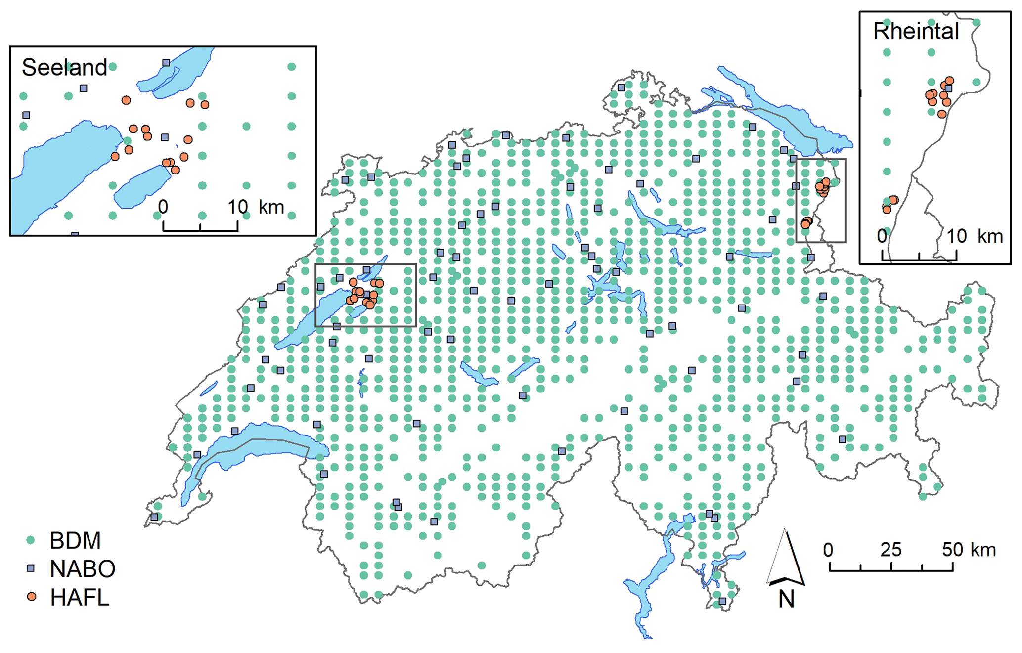
Figure 1Spatial grid of BDM locations (green dots), NABO long-term monitoring locations (gray squares) and the purposive sampling design of peatlands in the Seeland and St. Galler Rheintal regions, which constitute the HAFL locations (orange dots; NABO, 2018; Gubler et al., 2015; FOEN, 2018; Meuli et al., 2017; Baumann et al., 2021).
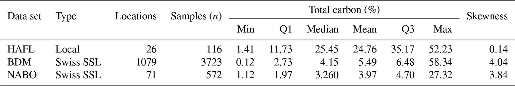
Table 1Summary statistics of all samples in the HAFL data set, which is, in this study, also referred to as the local data set, and the BDM and NABO data sets. The latter two together constitute the current Swiss SSL, which contains carbon reference measurements from 4295 samples from 1150 different locations (Baumann et al., 2021). Q1 and Q3 refer to the first and third quartiles, respectively.
We introduce a data set from the Bern University of Applied Sciences, School of Agricultural, Forest and Food Sciences (HAFL), which was set up using a purposive sampling design to specifically study drained peatlands and organic soils. This local HAFL data set (n = 116) contains soil samples from between 0 and 2 m depth from a range of natural and disturbed Histosols from 26 different locations in the Seeland and St. Galler Rheintal regions of Switzerland (Fig. 1 and Table 1; IUSS Working Group WRB, 2014). These samples originate from either undisturbed and waterlogged organic horizons, mineralized organic horizons under agricultural use, horizons with sandy or calcareous substrate material or horizons containing a mixture of these characteristics.
2.2 Mid-IR soil spectroscopy measurements and preprocessing
All samples were dried, sieved (<2 mm) and finely ground using a ball mill to maximize the signal-to-noise ratio (Guillou et al., 2015). The samples were measured with a VERTEX 70 Fourier-transform infrared (FTIR) spectrometer with a high throughput screening extension (HTS-XT) from Bruker (Massachusetts, USA). We used a spectral range of 7500 to 600 cm−1 and a spectral resolution of 2 cm−1 so that each spectrum comprised of reflectance values at 6901 wavelengths. On each 24-well plate, there is a fixed gold panel as the reflectance background, and three NABO standards and two subsamples of 10 different samples were measured using the HTS-XT extension. This means that 10 samples with two different measurements were analyzed per plate, maximizing the signal-to-noise ratio by averaging the two measurements. Reflectance spectra were transformed to apparent absorbance and recorded as such. OPUS software was used for correcting atmospheric water and CO2.
We tested several preprocessing steps in order to increase the information content for modeling and to reduce the collinearity between consecutive wavelengths. We tested using a Savitzky–Golay (SG) filter with a first and second derivative, as well as a first-, second- and third-order polynomial (Savitzky and Golay, 1964). The window size (resolution) of 35 variables (70 cm−1) was kept constant. Instead, we tested different resolutions by selecting either all variables, every fourth or every eighth variable to reduce collinearity and redundancy among predictors. The combination of preprocessing steps used for all final modeling approaches was chosen that resulted in the lowest root mean squared error (RMSE) across the cross-validated calibration (see Sect. 2.4 below).
We used the simplerspec package for the R statistical language for reading spectra and metadata from Bruker OPUS binary files into a R list, gathering spectra into a data structure of a list, resampling spectra to new wavenumber intervals, averaging spectra of replicate scans and preprocessing the raw spectra with the parameters described above (Baumann, 2020).
2.3 Reference chemical analysis
In order to guarantee that reference data for all mid-IR spectroscopy models were measured using the same standard soil chemical analysis methods, we prepared and measured SC in the local HAFL data set using the same procedures as for the Swiss SSL (Baumann et al., 2021). Briefly, all the dried, sieved (<2 mm) and finely ground samples were measured for total carbon content by dry combustion, using the CHN628 Series Elemental Determinator from the Laboratory Equipment Corporation (LECO Corporation, St. Joseph, MI, USA). We used a soil standard sample with a mean total carbon content of 2.372 %. In order to compare the measurement accuracy and accordance between the two different CHN628 Series Elemental Determinator machines used for the Swiss SSL and HAFL samples, representative samples were selected using a two-step process. The data were separated into two clusters using the K-means clustering algorithm (Hartigan and Wong, 1979), followed by using the Kennard–Stone (KS) algorithm for each cluster separately (Kennard and Stone, 1969). The KS algorithm is a deterministic approach that uses Euclidean or Mahalanobis distance to select a set of samples uniformly distributed in principal component (PC) space (Kennard and Stone, 1969). Within the Swiss SSL, NABO and BDM samples used the same machine (Baumann et al., 2021).
2.4 Spectroscopic modeling
We resampled the data using five repetitions of a location-grouped, 10-fold cross-validation for all of our models to determine the optimal number of components in model tuning, as well as evaluating the model performance using the hold-out samples. The predicted carbon content was calculated in each model using the hold-out values of the measured, preprocessed and averaged mid-IR spectra. For the final models, the calculated average (mean) predictions over these five repetitions with the chosen number of components are shown. To avoid overfitting, we used the one standard error rule, i.e., instead of choosing the tuning parameter associated with the lowest RMSE, we chose the simplest model within one standard error (SE) of the empirically optimal model (e.g., Hastie et al., 2009).
We used partial least squares regressions (PLSRs; e.g., Wold, 1975; Wold et al., 1983, 1984, 2001) to predict SC. We tuned the PLSR using 1 to 10 components, and the final model for the number of components was chosen according to the one SE rule.
All spectroscopic models were evaluated for their performance using the RMSE, the ratio of performance to deviation (RPD; Williams and Norris, 1987, Eq. 5), the ratio of performance to interquartile range (RPIQ), the bias and R2. The RPD is suitable for normal distributions, while the RPIQ is more suitable for non-normal distributions (Bellon-Maurel et al., 2010). Since different definitions of R2 exist, we used the equation of the mean squared error skill score (SSmse; Wilks, 2011), also known as the model efficiency coefficient (MEC; Nash and Sutcliffe, 1970) to indicate the R2.
Given the large range of SC in these data sets, we also assessed the RMSE, RPD and RPIQ by increments of 10 % SC for all model validations. Hence, we calculated these metrics for all samples for which the measured SC values are between 0 % and 10 % SC, 10 % and 20 % SC and so on. In this manner, we expected to detect for which range of SC prediction error increases or decreases.
One advantage of repeated cross-validation is that model imprecision can easily be assessed for each prediction () using the standard deviation (SD) and mean () of the predictions across five repetitions, respectively. In this study, the SD is shown as error bars for each prediction () and was also calculated for each overall summary statistic assessing the model performance.
2.5 Calibration schemes
2.5.1 Local models
Spectroscopy becomes time- and cost-efficient when minimizing the amount of laborious chemical reference analysis. Therefore, it makes sense to split the local HAFL data into a calibration and validation subset (Fig. 2). In this manner, the validation can be used to determine how many samples are needed to accurately and precisely calibrate a model. We selected n=15, 20, 25, 30, 40, 50 and 58 representative local HAFL calibration samples by using the KS algorithm for the first five PCs. We did not build models using less than 15 samples. These selected samples were then used to calibrate iterations of PLSR models (Fig. 2). In an application of the method described, reference data would only have to be measured for the selected samples used for calibration. Each calibrated model iteration was validated using the same 58 remaining local samples never used for any of the calibration iterations.
2.5.2 SSL spiked models
In the next step, we utilized the Swiss SSL in iterations of model calibrations to see if predictive performance can be improved while further reducing the number of new local samples needed for reference analysis (Fig. 2). Also, we expected a large amount of additional data from the SSL to improve model robustness and reliability (Lobsey et al., 2017). With the help of all SSL samples containing carbon reference data (n = 4295), we were able to include iterations of PLSR calibrations spiked with as few as n=3, 5, 7 and 10 local HAFL samples. Further iterations with the same , 25, 30, 40, 50 and 58 local HAFL samples as for the local models were also calibrated. Just as with the local models, each iteration was validated using the same 58 remaining local samples never used for any of the calibration iterations.
2.5.3 Models using RS-LOCAL subsets
In the third approach, we tested whether representative subsets of the SSL using the RS-LOCAL algorithm improved the accuracy of predicting SC of the local HAFL samples (Fig. 2). The RS-LOCAL algorithm was used to data-mine the SSL for samples suitable for local or location-specific calibrations according to similarities of spectral signatures between the local HAFL and SSL soil samples (Lobsey et al., 2017). Local HAFL samples were selected in the same manner as in local and SSL spiked models, resulting in iterations of the same samples as before (Fig. 2). This variable was defined in the RS-LOCAL algorithm as m (Lobsey et al., 2017); so, in our case, m=3, 5, 7, 10, 15, 20, 25, 30, 40, 50 and 58 for each respective iteration. RS-LOCAL used m data to resample, evaluate and then remove irrelevant data from the SSL so that only the most appropriate data for deriving a local calibration remained in a new SSL subset K. K and m together formed a RS-LOCAL data set, which was used for a calibration. In addition to the SSL and m data, three parameters were needed for RS-LOCAL as follows (Lobsey et al., 2017):
-
k – the number of SSL samples randomly selected in the resampling step and also the target number of SSL samples returned by the algorithm
-
b – the number of times each sample in the SSL was tested, on average, in each iteration of the algorithm
-
r – the proportion of SSL samples removed in each iteration of the algorithm.
In order to optimize the tuning parameters, we performed a full factorial combination of k (50, 100, 150 and 300), b (40, 50 and 60) and r (0.05 and 0.01) based on recommendations of the developers (Lobsey et al., 2017). The size of K remains the same for all values of m, only as long as k, b, r and the size of the entire SSL remain constant. As in the other modeling approaches, each iteration was validated using the same 58 remaining local samples never used for any of the calibration iterations.
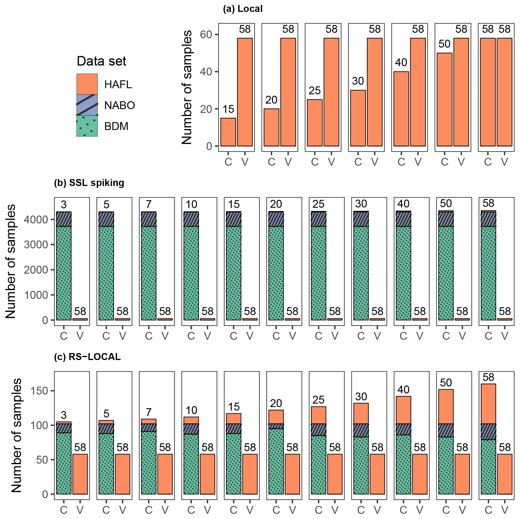
Figure 2The number of samples used in each calibration (C) and validation (V) scheme using HAFL, BDM and NABO data sets for (a) local, (b) SSL spiking and (c) RS-LOCAL approaches. The same 58 local HAFL samples never used in calibration were used to validate each modeling approach and iteration. Note different the scales on the y axes.
3.1 Spectral preprocessing and analysis of local HAFL spectra
The lowest RMSE was achieved in the cross-validated calibration when using a SG filter with a first derivative and second-order polynomial (Savitzky and Golay, 1964) in combination with a window size of 35 points (70 cm−1) and selecting only every eighth variable. This resulted in 209 variables between 634 and 3962 cm−1, which formed the predictors for subsequent modeling. Reducing the number of variables did not have an effect on model performance but reduced collinearity and redundancy, increased the simplicity of the model and decreased the computation time (Appendix A). An example of the PLSR tuning based on the number of chosen components in each repetition according to the one SE rule is shown using all local HAFL samples in Appendix B.
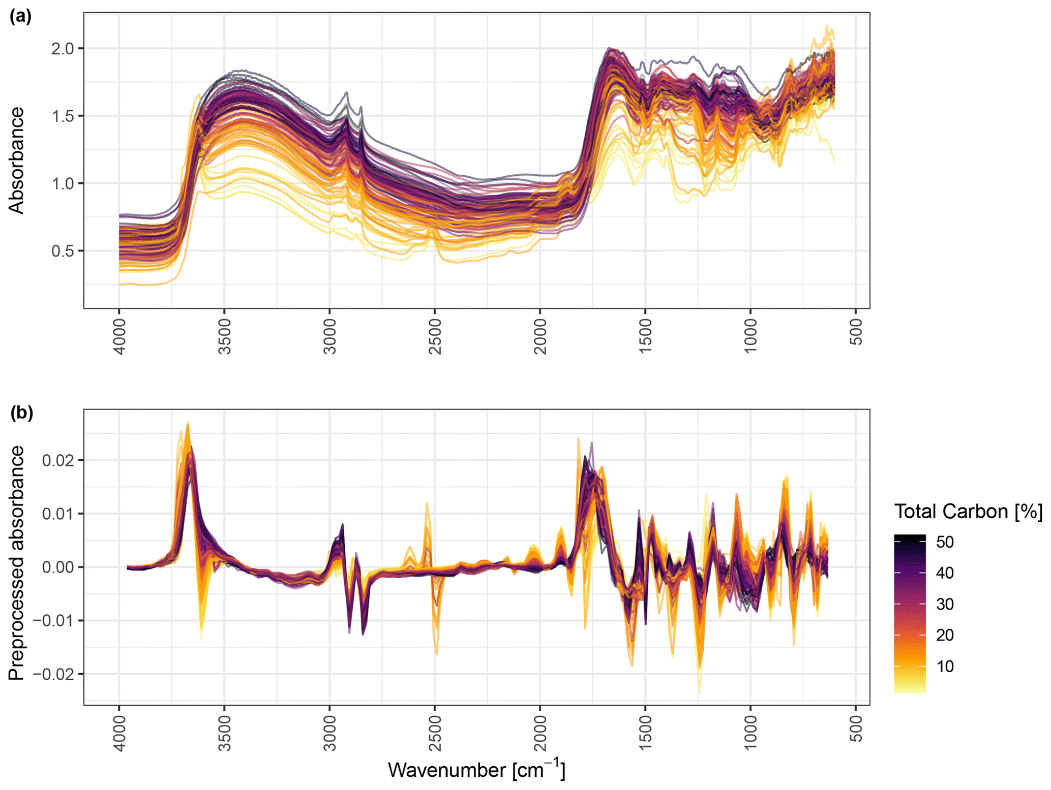
Figure 3The raw (a) and preprocessed (b) mid-IR spectra of all the local HAFL soil samples (n = 116) colored by total carbon content (percent).
The raw and preprocessed measured mid-IR spectra of the local HAFL soil samples (n = 116) were clearly distinct in relation to the SC content, ranging from 1 % to 52 % (Fig. 3a and b). Mineral and organic soil samples showed different absorbance patterns in both the raw and preprocessed mid-IR spectra. Preprocessed absorbance values showed a clear pattern according to the SC content almost across the entire spectrum and particularly, but not exclusively, around 800, 1050, 1900, 2050, 2900 and 3600 cm−1.
A principal component analysis (PCA) of the preprocessed spectra of the local HAFL samples clearly revealed a variance in the distribution of the soil samples related to the SC content (Fig. 4). The first two PCs together explained 53.5 % of the total variance in the preprocessed spectra. Figure 4 also exemplifies one possible local calibration scheme, whereby the HAFL data is split into 20 representative samples used for calibration, 58 samples used for validation and the remaining samples. We also compared the similarity of soil samples from different depths at the same location by coloring the first two PCs by location (Appendix C). However, the preprocessed spectra from the same locations generally showed little similarity; there was no distinct pattern as there was for the SC content.

Figure 4PC1 vs. PC2, computed via scaled and centered PCA, of the preprocessed local HAFL soil spectra (n = 116) colored by total carbon content (percent). The axes labels show the relative amount of variance explained (percent) in parentheses. In this example, n = 20 representative samples were selected using the KS algorithm for calibrating a local model.
3.2 Comparing local HAFL to SSL data
When comparing the three data sets, we found that the local HAFL data set showed a different SC distribution and covered a different range in soil variability than the Swiss SSL (Table 1 and Fig. 5). The relatively small HAFL data set originating from peaty soils had a uniform continuous distribution, whereas the BDM and NABO data had a positively skewed distribution with regard to SC (Table 1). Although the BDM data set contained the highest single value of SC, over 98 % of soil samples in the Swiss SSL originated from mineral soils. In contrast, more than half of the HAFL samples ranging from 1 % to 52 % were classified as organic soils. The first and second PCs – which together covered 40.3 % of the total variance – also revealed a clear overlap of preprocessed mid-IR absorbance variance for the BDM and NABO data sets (Fig. 5). There was less overlap in the variance of the preprocessed mid-IR absorbance values of the Swiss SSL and the HAFL data set. In the PCA space, the BDM and NABO data sets show a similarly shaped convex hull and almost identical centroid (mean), whereas the centroid is very distinct for the HAFL data set (Fig. 5). In Fig. 5, 122 samples, of which 20 are the local HAFL samples, were used as a RS-LOCAL subset to calibrate a model.
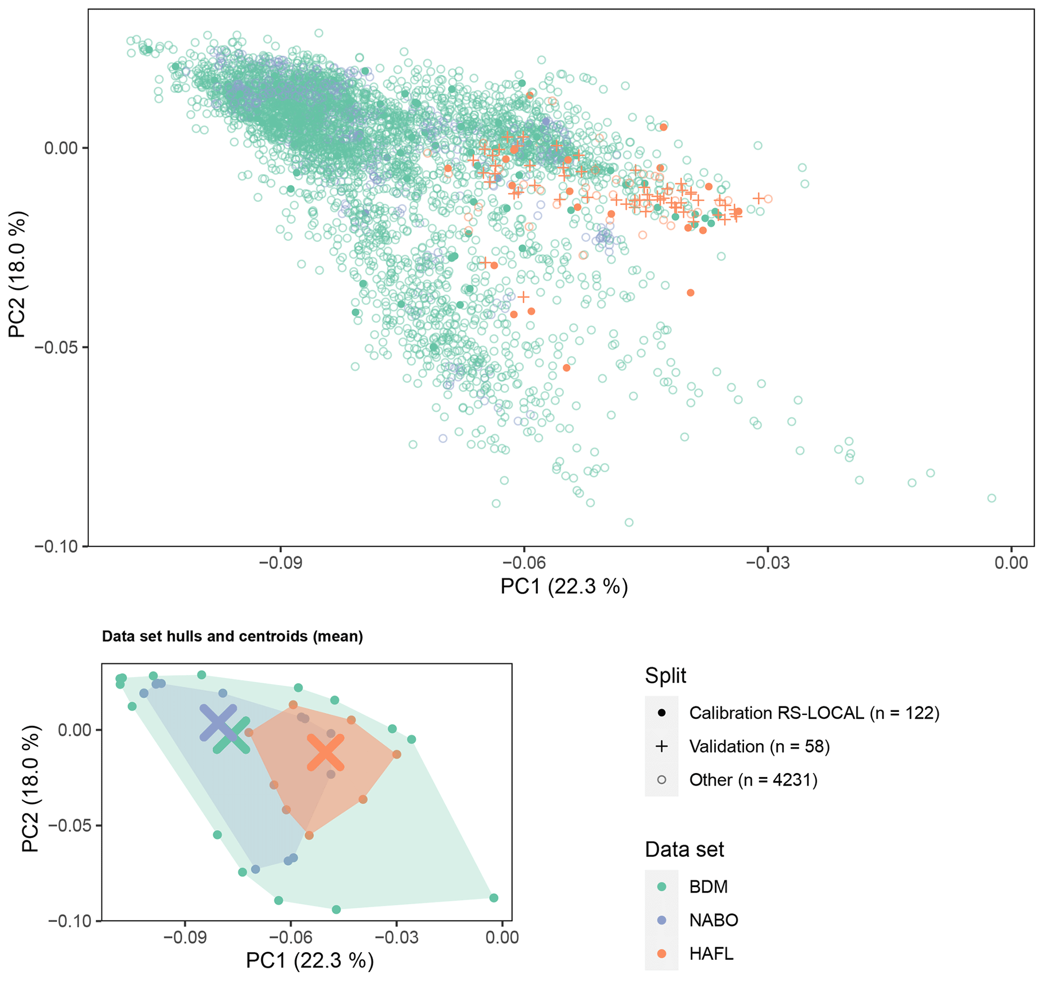
Figure 5PC1 vs. PC2 and the convex hulls and centroids (mean) in the PCA space of the preprocessed soil spectra of the local HAFL data set (n=116) and the BDM and NABO data sets, which make up the current Swiss SSL (n = 4295). Here, the PCs were computed via unscaled and uncentered PCA, since it showed the data distribution better than a scaled and centered PCA. The axes labels show the relative amount of variance explained (percent) in parentheses. In this example, the same representative local HAFL samples (n = 20) selected in Fig. 4 were used by RS-LOCAL to subset representative samples from the SSL (n = 102), which were used together for model calibration (n = 122).
3.3 Predicted SC using (1) local, (2) SSL spiking and (3) RS-LOCAL subsets
We predicted SC content () of the HAFL, BDM and NABO data sets using mid-IR soil spectroscopic PLSR models and compared them to the reference chemical measurements (Y). This is exemplified for each modeling approach in the case of 20 local HAFL samples in Fig. 6. For models using an RS-LOCAL subset, we found the best overall validation results using k=100, b=50 and r=0.05 and, therefore, chose these parameter values for all results shown here. The influence of RS-LOCAL parameter k on validation results is shown in Appendix D. Decreasing r to 0.01 had little influence on model performance and greatly increased the computation duration. There appeared to be no spatial correlation between chosen RS-LOCAL locations and target HAFL locations (Appendix E).
For calibration, all modeling approaches showed a high fit (R2>0.9) and low overall bias (≈0; Fig. 6a). The SSL spiking calibration scheme showed the lowest RMSE value. However, the accuracy of the spiked SSL calibration decreased and bias increased in the upper range of SC, which also explains the lower RPIQ value compared to local and RS-LOCAL calibration schemes. The RS-LOCAL calibration revealed the best model performance according to the RPD (6.92). The local PLSR, using only 20 samples, showed the lowest overall calibration accuracy based on the RMSE (3.72 % total carbon).
All model validations showed a similar fit (R2 = 0.93 to 0.97). However, the bias, RMSE, RPD and RPIQ values differed among the three scenarios (Fig. 6b). The validation of the local PLSR had the lowest bias (0.53), but the validation of the RS-LOCAL subset had the best performance overall (RMSE = 2.82 % total carbon, RPD = 4.67 and RPIQ = 6.82). The validation of the spiked SSL scheme revealed the lowest prediction accuracy overall, especially with increasing values of measured SC. The error bars representing the SD of predictions across five resampled repetitions showed that there was the highest prediction uncertainty across repetitions in the validation of the local modeling approach. As with 20 local samples, validation statistics also show a good performance of PLSR models using RS-LOCAL subsets that contained as few as 5, 7 and 10 local samples (R2 = 0.93 to 0.96; bias = 0.2 to 1.651; RMSE = 2.71 % to 3.89 % total carbon; RPD = 3.38 to 4.86; and RPIQ = 4.93 to 7.09; Appendix F).

Figure 6Predicted () vs. observed (Y) total carbon content (percent) by calibrating a PLSR with 20 local HAFL samples (a) and validating it with the remaining local HAFL samples (n=96) (b). A PLSR was calibrated using only 20 local HAFL samples (1), adding the entire SSL to the 20 local HAFL samples (2) and using a RS-LOCAL subset of the SSL also containing the 20 local samples (3). The error bars signify the SD, and where none are present, the components remained identical across five repetitions and, thus, SD =0.
We compared R2, bias, RMSE, RPD and RPIQ as indicators of overall model performance depending on the number of local HAFL samples in each calibration scheme for all three modeling approaches, i.e., (1) local, (2) SSL spiking and (3) RS-LOCAL subsets (Figs. 7 and 8). R2 was a poor indicator of model performance and did not show substantial differences between modeling approaches and calibration schemes (Fig. 7). Local models showed the lowest bias, regardless of the number of samples used during calibration (Fig. 7). The bias of validations of spiked SSL models only lowered slightly as the number of local samples was increased and remained large overall (>3). Bias was reduced significantly in validated models of RS-LOCAL subsets when at least five local samples were included and continued to decrease slightly with the increasing number of local samples. Models with five and 10 samples stand out with very little bias.
Model accuracy (RMSE) varied considerably between calibrations and validations when SSL samples were used during calibration (Fig. 7). There was less of a difference between calibration and validation in local models, where the RMSE decreased with the increasing number of local samples in model calibration. As with model bias, the RS-LOCAL subsets again showed a threshold or minimum of five samples in order for the RMSE of model validations to lower significantly. Model validations of local and RS-LOCAL subsets showed very similar accuracy overall (RMSE ≈ 3 % total carbon). However, only five or 10 local samples were required to achieve an accuracy of RMSE = 3.16 % or 2.71 % SC, respectively (Fig. 7 and Appendix F). In contrast, local modeling approaches required 50 local samples to achieve a RMSE of <3 % SC.
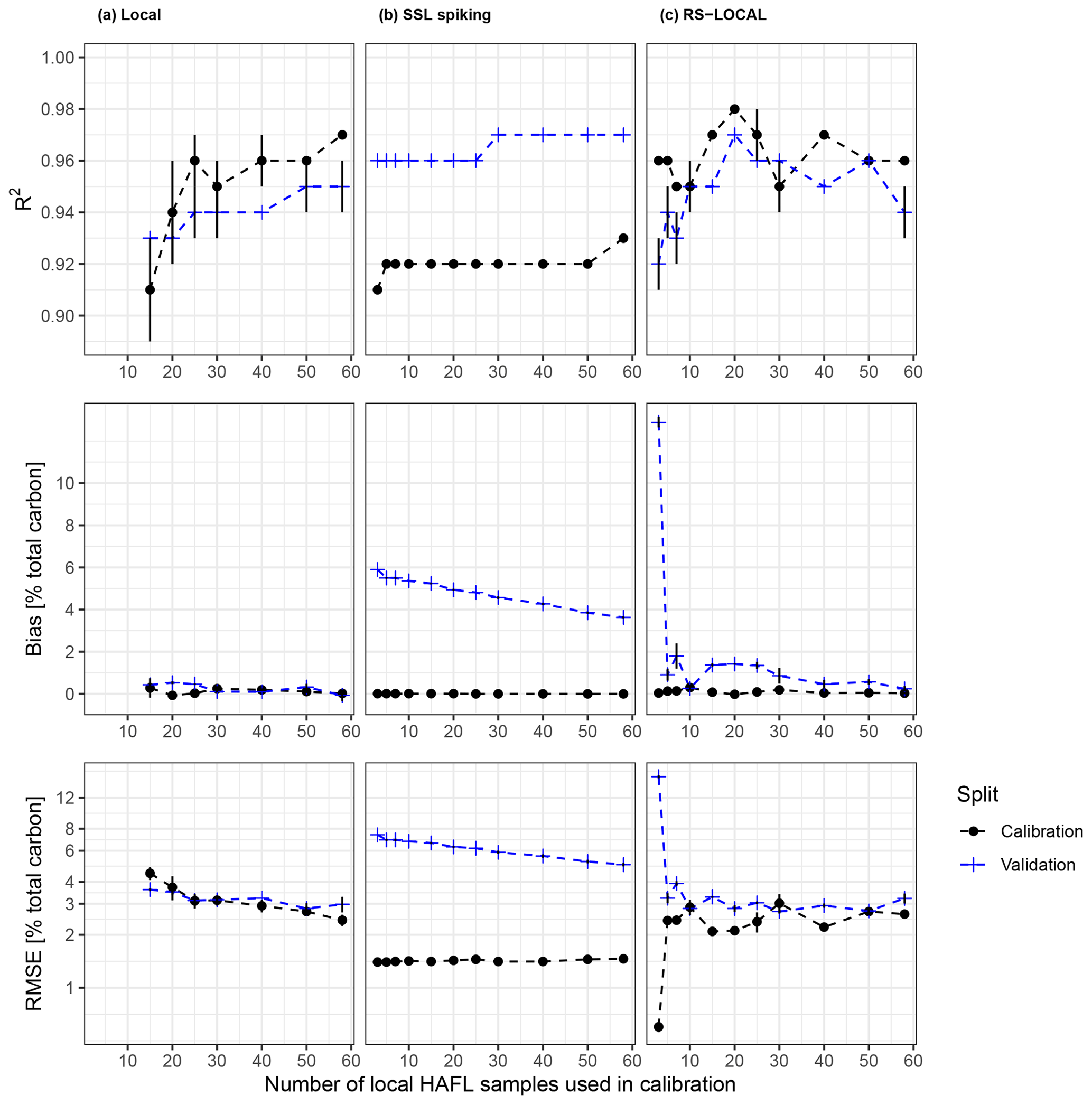
Figure 7R2, bias and RMSE values in percent of total carbon (RMSE in logarithmic scale) vs. the number of local HAFL samples used in local HAFL (a), local combined with SSL (b) and RS-LOCAL subsets (c), where k = 100. Error bars represent the SD between resampled repetitions, and where not present, there was no variation in the respective summary statistic across five repetitions. Dashed lines between data points do not represent real measurements and are only for visual guidance.
Local and RS-LOCAL models also revealed similar and better model performance than SSL spiking modeling approaches (Fig. 8). Both RPD and RPIQ gradually increased in local models with increasing numbers of local HAFL samples in calibration. As with bias and RMSE, RPD and RPIQ values also indicate high-prediction accuracy with as few as five or 10 local HAFL samples when calibrating with RS-LOCAL subsets (RPD = 4.08 and 4.66 and RPIQ = 5.96 and 6.81, respectively).
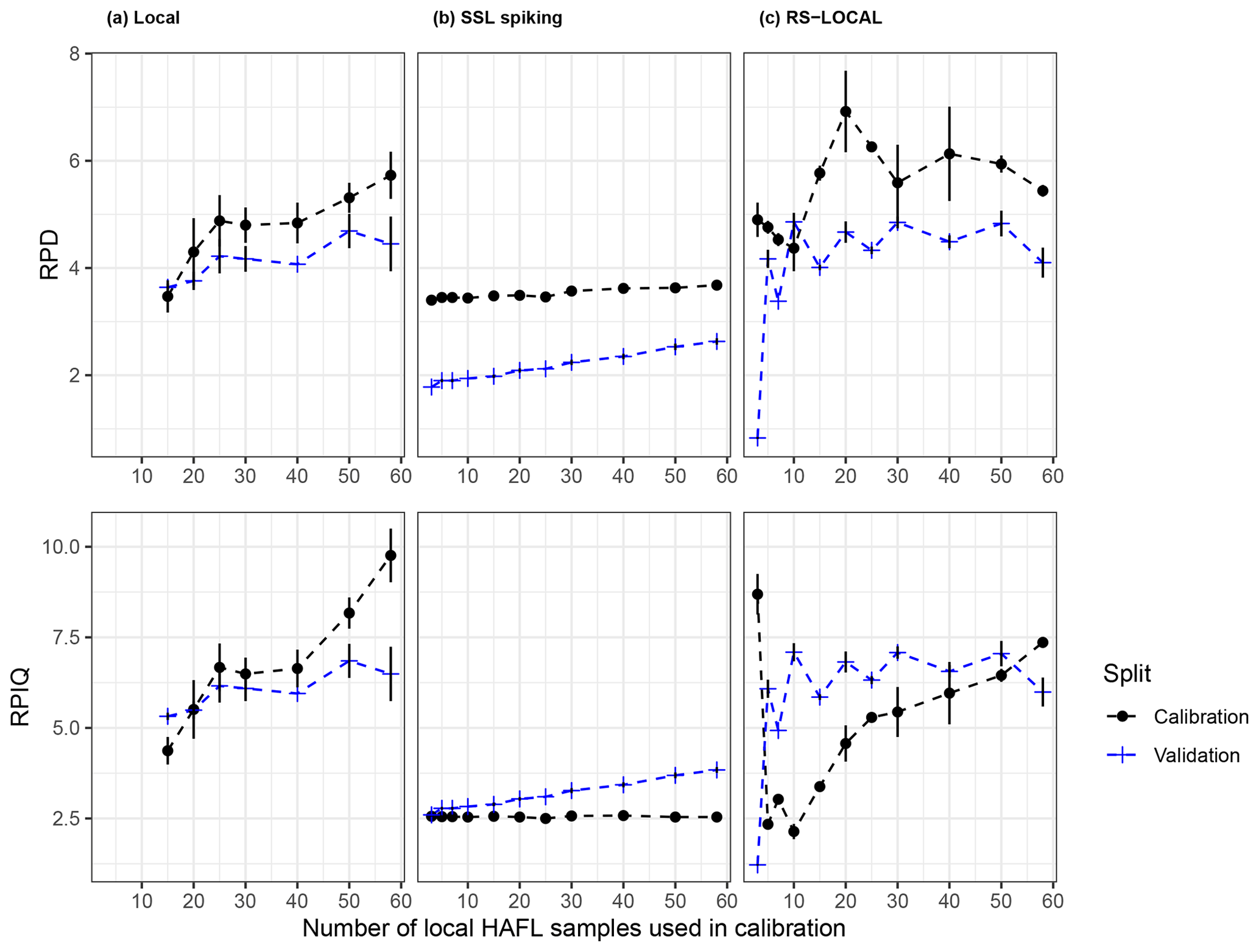
Figure 8RPD and RPIQ vs. the number of local HAFL samples used in local HAFL (a), local combined with SSL (b) and RS-LOCAL subsets, where k = 100 (c). Error bars represent the SD between resampled repetitions, and where not present, there was no variation in the respective summary statistic across five repetitions. Dashed lines between data points do not represent real measurements and are only for visual guidance.
Prediction accuracy in model validations was highest for mineral soils, or ranges of SC between 0 % and 20 % for all modeling approaches (Fig. 9). Local and RS-LOCAL modeling approaches showed better predictive performance for samples with higher SC. In local modeling approaches, samples with 0 % to 20 %, and especially 10 % to 20 % SC, were predicted increasingly well with an increasing number of local HAFL samples in the model calibration. Soils between 0 % and 10 % SC were predicted with the highest accuracy with the SSL spiking approach. However, samples with > 10 % were predicted with higher accuracy using local and RS-LOCAL calibration schemes. Validations of RS-LOCAL calibration schemes again showed a threshold around five local HAFL samples. After this threshold, RMSE, RPD and RPIQ results for samples with > 20 % remained constant with an increasing number of local samples during calibration. In contrast, samples containing 0 % to 20 % SC were considerably more unstable, depending on the number of local samples during calibration.
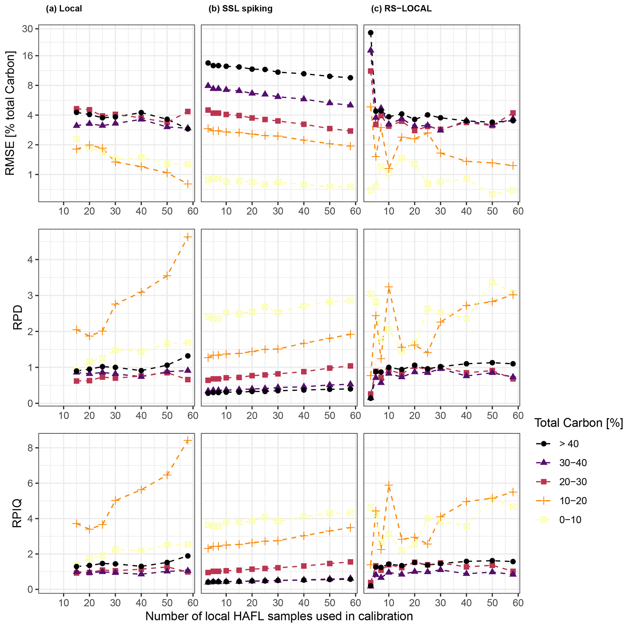
Figure 9RMSE (in percent of total carbon and logarithmic scale), RPD and RPIQ of validation results vs. the number of local HAFL samples used in local HAFL (a), local combined with SSL (b) and RS-LOCAL subsets (c), where k = 100. Observations (Y) were grouped in increments of 10 % SC, and the validation metrics were calculated separately for each group. Dashed lines between data points do not represent real measurements and are only for visual guidance.
We found that, first, mid-IR spectra can be used to predict SC up to 52 % with R2≥0.94, negligible bias and RMSE = 2.8 % to 3.6 % total carbon using validated local PLSR models (RPD = 3.6 to 4.69; RPIQ = 5.32 to 6.85). Second, and most importantly, time-consuming and expensive field and laboratory measurements can be reduced for new locations when using a SSL together with RS-LOCAL. In our study, only 10 local HAFL samples were required in a RS-LOCAL subset to achieve a similar validation performance as with at least 50 local samples in a local model (R2 = 0.96; bias ≈0.2; RMSE ≈ 2.7 % total carbon; RPD = 4.86; and RPIQ = 7.09; Figs. 7 and 8). This is a major improvement on local models without a SSL because not only does it reduce field and laboratory expenses but also because no reliable model can be calibrated using such little data. Furthermore, a SSL subsetting method, such as RS-LOCAL, combined with a simple model, such as PLSR, is easy to understand and requires little computational power compared to alternative machine or deep learning approaches (e.g., Padarian et al., 2019a, b).
4.1 Spectral patterns reflect mineral and peat composition
The measured and preprocessed mid-IR soil spectra and PCA results of all local HAFL samples revealed a high correlation between the spectral absorbance values and a broad range of SC content overall (Figs. 3 and 4). According to past studies that assessed variable importance, we assumed that soil texture and mineralogical and organic composition influence mid-IR spectral absorbance the most (Madari et al., 2006; Bornemann et al., 2010; Calderón et al., 2011). SOC (soil organic carbon), for example, is known to be related to a variety of bands that represent absorptions due to organic molecules such as proteins with C–O, C=O and N–H bonds (Viscarra Rossel and Behrens, 2010). Local HAFL samples containing both a high number of organic compounds and carbonates created distinct absorbance bands around 1450, 1460, 2855 and 2930 cm−1 for aliphatic C–H constituents (Madari et al., 2006) or around 1320 cm−1 for hydroxyl groups bonded to carbon (C–O–H) (Bornemann et al., 2010) and around 2500 cm−1 for carbonates (Calderón et al., 2011). Future studies should investigate whether the overlapping of spectral signals for organic and mineral components increases at high SC concentrations implies that spectral absorbance patterns above a certain threshold of SC no longer differentiate substantially.
4.2 RS-LOCAL improves model performance and increases efficiency
The RS-LOCAL approach, using representative local and SSL samples, was found to be the best of the three compared approaches. It significantly reduces the number of reference measurements that need to be made at new locations for five samples. In addition, the RS-LOCAL approach helps remove the strong bias of spiked SSL calibrations (Figs. 6 and 7), increasing the underestimated predictions of SC in the upper range. Finally, the additional samples provided from the SSL also reduce the uncertainty of SC predictions of resampled repetitions in the PLSR models, as can be seen from the smaller error bars of the residuals. Predictions of SC from 0 % to 10 % became more accurate when using additional samples from the SSL in the RS-LOCAL subset (Fig. 9).
We postulate that SC prediction accuracy of organic soil samples, using SSL-derived models, may be improved in future studies by adding more peat soil data to the Swiss SSL (Baumann et al., 2021), specifically for samples at different decomposition and mineralization stages. One of the most important characteristics of a high-quality SSL is that it contains the highest possible variation in soil characteristics within its designated area (Viscarra Rossel et al., 2016a). The SC distribution and the spectral principal component space of the HAFL compared to the BDM and NABO samples showed that the soil variability in the HAFL samples is only marginally covered by the current SSL (Table 1 and Fig. 5).
The use of our modeling approach, the PLSR of RS-LOCAL subsets, to predict soil properties at new locations for future studies and applications depends on the level of accuracy needed. For organic soils on a farm or landscape level, an accuracy of approximately 2 % to 3 % total carbon is suitable for quantifying SC. On the one hand, this range of accuracy is not useful for mineral soils, which, in Switzerland for example, contain average (mean) topsoil SOC concentrations of 2 % on arable locations and 2.5 % on temporary grassland locations (Leifeld et al., 2005). On the other hand, our validation results using the SSL spiking approach show that samples with 0 % to 10 % SC were constantly predicted with a RMSE < 1 % SC and RPD above 2 (Fig. 9). This implies that, when targeting mineral agricultural soils, mid-IR spectroscopic models making use of a SSL deliver the required accuracy for applications and end-users. These findings are supported by Baumann et al. (2021).
Few studies, to our knowledge, have predicted organic soils up to 52 % total carbon using mid-IR soil spectroscopy without splitting model calibration for mineral and organic soils. One exception is the mid-IR SSL of the United States, which contains about 2000 organic soil samples (Wijewardane et al., 2018; Dangal et al., 2019). Nocita et al. (2014) predicted SOC for croplands, grasslands, woodlands and organic soils separately from about 20 000 samples from the Land Use/Cover Area frame Survey (LUCAS) across Europe using vis-NIR spectroscopy. For the model using only organic soil data with a range of 12.0 % to 58.68 % SOC, predictions were less accurate (RMSE = 5.114 % SOC) than in this study (Nocita et al., 2014).
One advantage of the RS-LOCAL–PLSR approach used here is that the statistical modeling is simple and produces easy-to-understand models compared to other transfer and deep learning approaches (Padarian et al., 2019a, b). Using spectral- or model-based information from SSLs by spiking, subsetting and memory, instance and transfer learning may even be beneficial for parts of the world lacking legacy soil data or funding to establish their own SSL. In other words, the SSL of one region may be used to predict locally for another region that does not have a SSL. This is comparable to the concept of homosoil in digital soil mapping (Mallavan et al., 2010).
However, there are still some drawbacks. As mentioned by Padarian et al. (2019a), spiking and subsetting are dependent on the size of local and global data sets and may still bias the predictions towards the local data set rather than fully using valuable global information, which generates less robust models. Although transfer learning of model rules, or network weights, showed promising results on a continental scale (Padarian et al., 2019a), it has not been tested when transferring national spectral knowledge to a field scale.
Ultimately, soil spectroscopy has the potential to speed up the quantification of soil properties for soil mapping and monitoring. Several studies have shown how this affects soil maps and associated uncertainties (Brodský et al., 2013; Viscarra Rossel et al., 2016b; Ramirez-Lopez et al., 2019) but only on a farm scale. It still remains to be implemented in a large-scale soil information system.
This study reveals that, if adequately mined, the information in a SSL is sufficient to predict soil carbon of a new study region with very different soil characteristics. Whereas past spectroscopy studies mostly focused on mineral soils, these model validations of SC ranging between 1 % to 52 % show that using as few as five new samples, in combination with RS-LOCAL and a SSL, yield promising results. This approach decreases the time and cost of field and laboratory soil analysis, reduces the bias of large-scale spectroscopy or SSL spiked models and the uncertainty of small-scale local models. Including more organic soil samples in the Swiss SSL will make it more robust for future modeling applications (Baumann et al., 2021). This case study for assessing SC in drained peatlands under agricultural management shows that an operative SSL is useful for scaling up quantitative soil information over space and time.
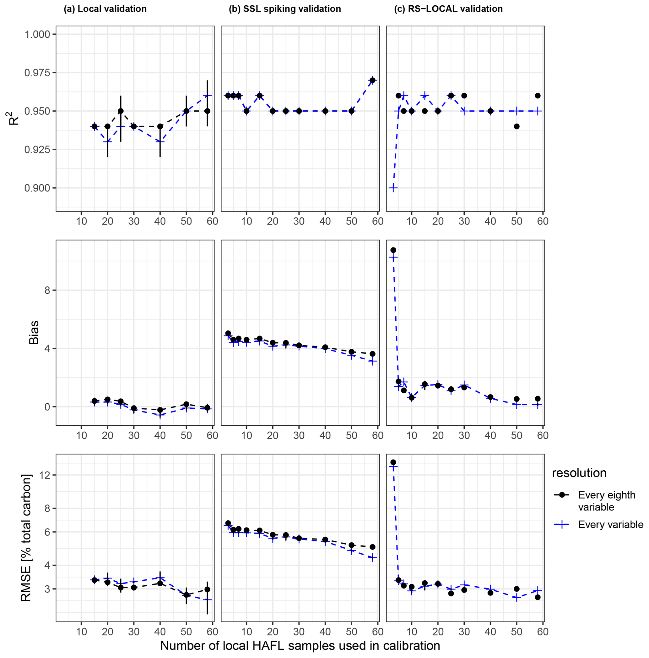
Figure A1R2, bias and RMSE values in percent total carbon (RMSE in logarithmic scale) of model validations vs. the number of local HAFL samples used in local HAFL (a), local combined with SSL (b) and RS-LOCAL subsets of the SSL (c), where k = 300 . These validation metrics are shown for models using all spectral variables as opposed to only every eighth variable, which is a preprocessing step.
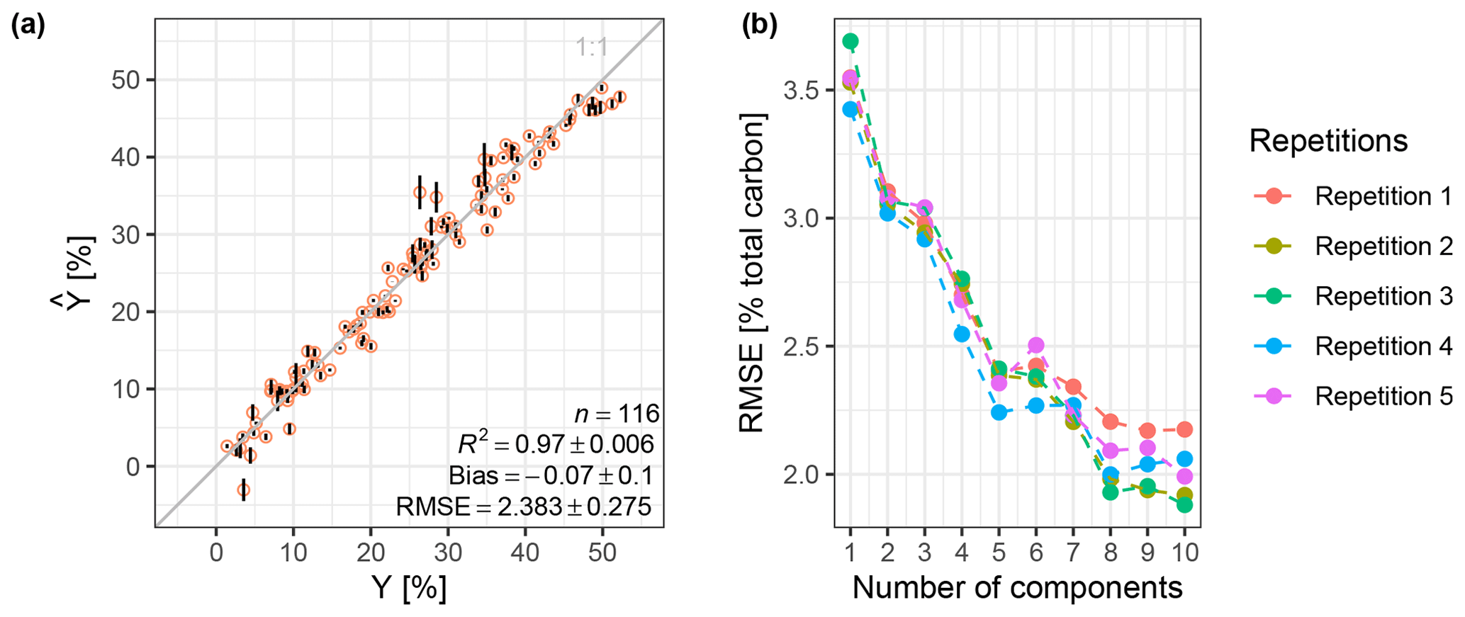
Figure B1(a) Predicted vs. observed Y total carbon (percent) of all local HAFL samples using a PLSR. (b) Illustrative example of PLSR tuning, showing the calculated RMSE (percent total carbon) vs. the number of components used in each repetition. This model used seven components in the first and fifth repetition and eight components in the second, third and fourth repetition, according to the one SE rule.
Local HAFL soil samples from different depths of the same location were diverse. This may be due to pedogenetic formation conditions unique to peatlands near bodies of water and anthropogenic influence. The Seeland and St. Galler Rheintal regions are characterized by an extreme diversity of intact peat, decomposed and mineralized peat, calcareous lacustrine sediments and fluvial sand, silt and clay deposits, depending on past river flow conditions (Bader et al., 2018; Burgos et al., 2018). Anthropogenic influences, such as changing the course of and channeling of rivers, lowering lake and groundwater tables and draining peatlands, further complicate soil characterization. These conditions create a mosaic of extremely heterogeneous soil characteristics that vary vertically, depending on soil depth, as strongly as they vary horizontally across the entire three study areas that are part of the HAFL data set (Fig. C1).
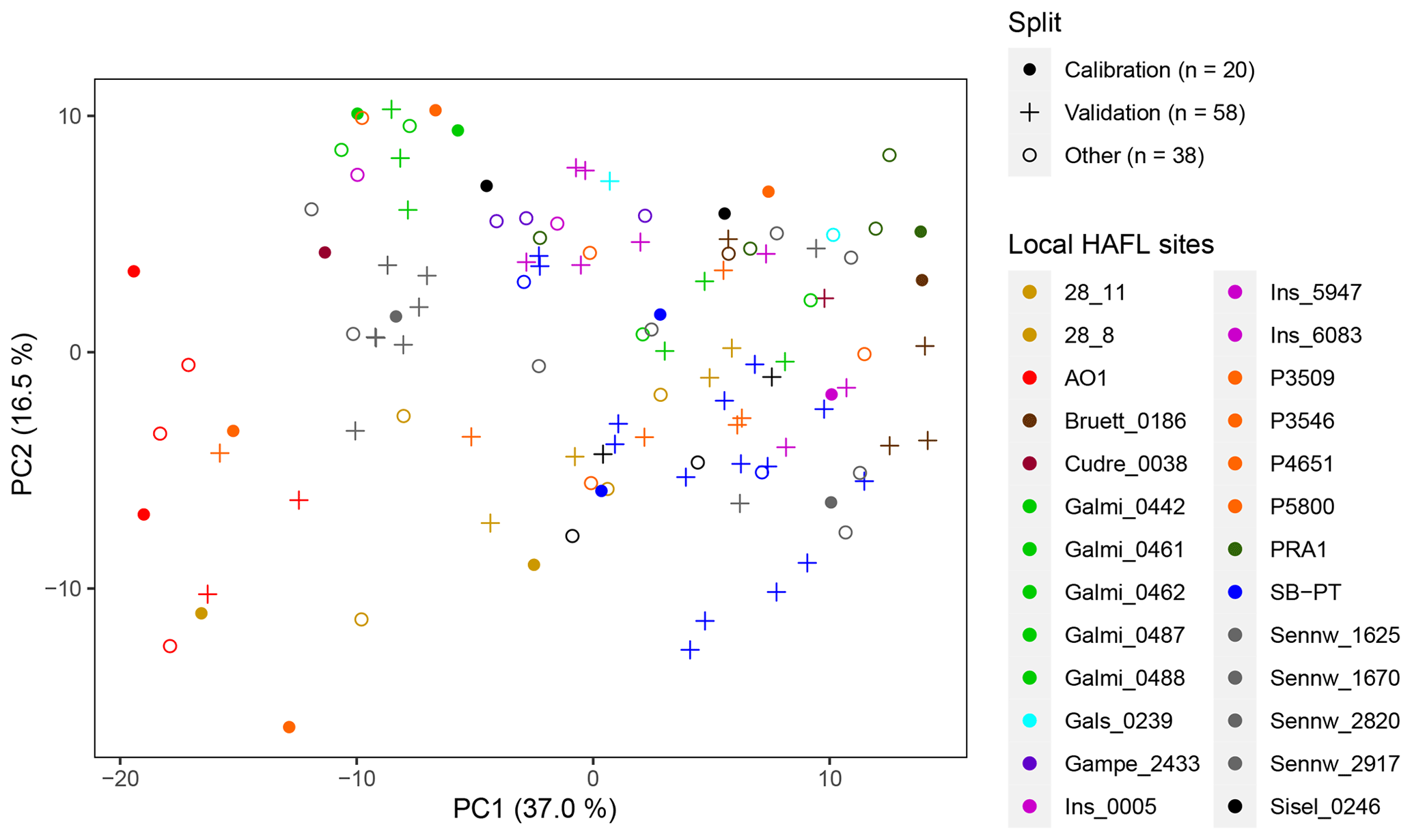
Figure C1PC1 vs. PC2, computed via scaled and centered PCA, of the preprocessed local HAFL soil spectra (n = 116) colored by location, in contrast to Fig. 4. The axes labels show the relative amount of variance explained (percent) in parentheses. In this example, n = 20 representative samples were selected for calibrating a local model using the KS algorithm, and the rest of the data were used for validation (n = 96).

Figure D1R2, bias and RMSE (percent total carbon) of the validation of RS-LOCAL modeling approaches, using different numbers of local HAFL samples in model calibration, when altering the RS-LOCAL parameter k. The RMSE is on a logarithmic scale.
We mapped the locations from which RS-LOCAL selected samples from the SSL for calibration together with 20 local HAFL samples (n = 334; k = 300; Fig. E1). There appeared to be no spatial correlation between chosen RS-LOCAL locations and geographical distance from the local HAFL locations. In other words, locations chosen by RS-LOCAL suggest that spectrally relevant soil samples from SSL for predicting SC in local HAFL samples are not confined to nearby areas in terms of geographical distance. This may be linked to the heterogeneity of soils found in these drained peatlands; in between layers of organic soils, sampled soil layers also contain geologic substrate material from lacustrine carbonates, dense clay or fluvial sand depositions. We speculate that this soil and spectral diversity at local HAFL sampling locations may explain why RS-LOCAL even selected relevant SSL samples originating from the Alps. This ultimately suggests that RS-LOCAL is able to use segments of soil spectra from a variety of similar but also dissimilar locations to predict new local soil samples.

Figure E1A map showing BDM (green dots) and NABO (gray squares) locations from which RS-LOCAL subset samples (n = 314, k = 300) for a RS-LOCAL calibration (n = 334). All HAFL locations (orange dots) are shown underneath BDM and NABO locations to allow a better focus on locations chosen by RS-LOCAL.
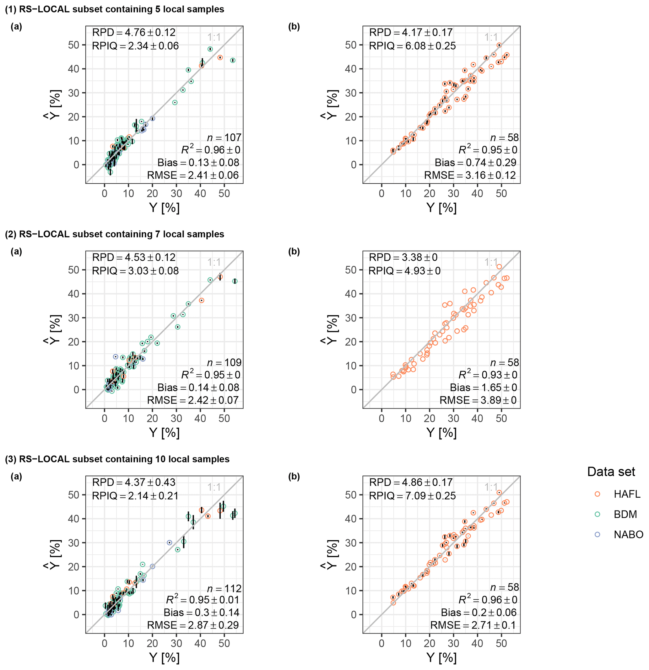
Figure F1Predicted () vs. observed (Y) total carbon content (percent) by calibrating a PLSR of a RS-LOCAL subset with five (1), seven (2) and 10 (3) local HAFL samples (a) and validating each with 58 local HAFL samples (b), respectively. The error bars signify the SD, and where none are present, the components remained identical across five repetitions and, thus, SD =0.
The data sets and code to reproduce the results of this paper are available upon request.
All authors contributed to the scientific research in this project and read through, edited and provided advice on improving the paper. AH measured all SSL and HAFL samples using mid-IR spectroscopy, performed the data preparation and analysis, wrote most of the R code and wrote the paper. Some of the R code was written by PB, and RS-LOCAL was implemented in R by RVR. AG provided the maps of sampling locations. SO collected and prepared the HAFL soil samples. JS helped with the interpretation of the results and improved the writing.
The authors declare that they have no conflict of interest.
We would like to thank the authors of Baumann et al. (2021) for the establishment of the Swiss SSL. We are grateful to Daniel Wächter and Reto Meuli from the Swiss Soil Monitoring Group at Agroscope for the consent to access, quality control and data manage both the milled soil samples and the database with reference measurements of the National Soil Monitoring Programme (NABO) and Swiss Biodiversity Monitoring programme (BDM) data sets. Many thanks to Stéphane Burgos and Madlene Nussbaum from the Bern University of Applied Sciences (BFH), who gave advice on the spectroscopic models and shared their knowledge of (drained) peatland soils. We would also like to thank Raphael Viscarra Rossel and Juhwan Lee for the valuable input and time spent at the Commonwealth Scientific and Industrial Research Organisation (CSIRO) in Canberra, Australia. Finally, we express our gratitude to the Swiss Federal Office of the Environment for commissioning and funding the soil analyses conducted within the BDM.
This research has been funded by ETH Zurich grants.
This paper was edited by Bas van Wesemael and reviewed by Jonathan Sanderman and one anonymous referee.
Araújo, S. R., Wetterlind, J., Demattê, J. A. M., and Stenberg, B.: Improving the Prediction Performance of a Large Tropical Vis-NIR Spectroscopic Soil Library from Brazil by Clustering into Smaller Subsets or Use of Data Mining Calibration Techniques, Eur. J. Soil Sci., 65, 718–729, https://doi.org/10.1111/ejss.12165, 2014. a
Bader, C., Müller, M., Szidat, S., Schulin, R., and Leifeld, J.: Response of Peat Decomposition to Corn Straw Addition in Managed Organic Soils, Geoderma, 309, 75–83, https://doi.org/10.1016/j.geoderma.2017.09.001, 2018. a
Baumann, P.: Simplerspec, GitHub, available at: https://github.com/philipp-baumann/simplerspec (last access: 12 November 2020), 2020. a
Baumann, P., Helfenstein, A., Gubler, A., Keller, A., Meuli, R. G., Wächter, D., Lee, J., Viscarra Rossel, R., and Six, J.: Developing the Swiss soil spectral library for local estimation and monitoring, SOIL Discuss. [preprint], https://doi.org/10.5194/soil-2020-105, in review, 2021. a, b, c, d, e, f, g, h, i, j
Bellon-Maurel, V., Fernandez-Ahumada, E., Palagos, B., Roger, J.-M., and McBratney, A.: Critical Review of Chemometric Indicators Commonly Used for Assessing the Quality of the Prediction of Soil Attributes by NIR Spectroscopy, TrAC Trends Anal. Chem., 29, 1073–1081, https://doi.org/10.1016/j.trac.2010.05.006, 2010. a
Bornemann, L., Welp, G., and Amelung, W.: Particulate Organic Matter at the Field Scale: Rapid Acquisition Using Mid-Infrared Spectroscopy, Soil Sci. Soc. Am. J., 74, 1147–1156, https://doi.org/10.2136/sssaj2009.0195, 2010. a, b
Brodský, L., Klement, A., Penížek, V., Kodešová, R., and Borůvka, L.: Building Soil Spectral Library of the Czech Soils for Quantitative Digital Soil Mapping, Soil Water Res., 6, 165–172, https://doi.org/10.17221/24/2011-SWR, 2011. a
Brodský, L., Vašát, R., Klement, A., Zádorová, T., and Jakšík, O.: Uncertainty Propagation in VNIR Reflectance Spectroscopy Soil Organic Carbon Mapping, Geoderma, 199, 54–63, https://doi.org/10.1016/j.geoderma.2012.11.006, 2013. a
Brown, D. J.: Using a Global VNIR Soil-Spectral Library for Local Soil Characterization and Landscape Modeling in a 2nd-Order Uganda Watershed, Geoderma, 140, 444–453, https://doi.org/10.1016/j.geoderma.2007.04.021, 2007. a
Burgos, S., Nussbaum, M., Tatti, D., Kellermann, L., and Oechslin, S.: Bodenkartierung St. Galler Rheintal, Zwischenbericht, Berner Fachhochschule, Hochschule für Agrar-, Forst- und Lebensmittelwissenschaften HAFL, Zollikofen, 2018. a
Calderón, F. J., Reeves, J. B., Collins, H. P., and Paul, E. A.: Chemical Differences in Soil Organic Matter Fractions Determined by Diffuse-Reflectance Mid-Infrared Spectroscopy, Soil Sci. Soc. Am. J., 75, 568–579, https://doi.org/10.2136/sssaj2009.0375, 2011. a, b
Cardelli, V., Weindorf, D. C., Chakraborty, S., Li, B., De Feudis, M., Cocco, S., Agnelli, A., Choudhury, A., Ray, D. P., and Corti, G.: Non-Saturated Soil Organic Horizon Characterization via Advanced Proximal Sensors, Geoderma, 288, 130–142, https://doi.org/10.1016/j.geoderma.2016.10.036, 2017. a
Clairotte, M., Grinand, C., Kouakoua, E., Thébault, A., Saby, N. P., Bernoux, M., and Barthès, B. G.: National Calibration of Soil Organic Carbon Concentration Using Diffuse Infrared Reflectance Spectroscopy, Geoderma, 276, 41–52, https://doi.org/10.1016/j.geoderma.2016.04.021, 2016. a, b, c
Dangal, S., Sanderman, J., Wills, S., and Ramirez-Lopez, L.: Accurate and Precise Prediction of Soil Properties from a Large Mid-Infrared Spectral Library, Soil Sys., 3, 11, https://doi.org/10.3390/soilsystems3010011, 2019. a, b, c, d
Demattê, J. A., Dotto, A. C., Paiva, A. F., Sato, M. V., Dalmolin, R. S., de Araújo, M. d. S. B., da Silva, E. B., Nanni, M. R., ten Caten, A., Noronha, N. C., Lacerda, M. P., de Araújo Filho, J. C., Rizzo, R., Bellinaso, H., Francelino, M. R., Schaefer, C. E., Vicente, L. E., dos Santos, U. J., de Sá Barretto Sampaio, E. V., Menezes, R. S., de Souza, J. J. L., Abrahão, W. A., Coelho, R. M., Grego, C. R., Lani, J. L., Fernandes, A. R., Gonçalves, D. A., Silva, S. H., de Menezes, M. D., Curi, N., Couto, E. G., dos Anjos, L. H., Ceddia, M. B., Pinheiro, É. F., Grunwald, S., Vasques, G. M., Marques Júnior, J., da Silva, A. J., Barreto, M. C. d. V., Nóbrega, G. N., da Silva, M. Z., de Souza, S. F., Valladares, G. S., Viana, J. H. M., da Silva Terra, F., Horák-Terra, I., Fiorio, P. R., da Silva, R. C., Frade Júnior, E. F., Lima, R. H., Alba, J. M. F., de Souza Junior, V. S., Brefin, M. D. L. M. S., Ruivo, M. D. L. P., Ferreira, T. O., Brait, M. A., Caetano, N. R., Bringhenti, I., de Sousa Mendes, W., Safanelli, J. L., Guimarães, C. C., Poppiel, R. R., e Souza, A. B., Quesada, C. A., and do Couto, H. T. Z.: The Brazilian Soil Spectral Library (BSSL): A General View, Application and Challenges, Geoderma, 354, 113793, https://doi.org/10.1016/j.geoderma.2019.05.043, 2019. a
Ferré, M., Engel, S., and Gsottbauer, E.: Which Agglomeration Payment for a Sustainable Management of Organic Soils in Switzerland? – An Experiment Accounting for Farmers' Cost Heterogeneity, Ecol. Econ., 150, 24–33, https://doi.org/10.1016/j.ecolecon.2018.03.028, 2018. a, b
FOEN: Biodiversity Monitoring Switzerland (BDM), available at: https://www.biodiversitymonitoring.ch/index.php/en/ (last access: 20 February 2020), 2018. a, b
Gholizadeh, A., Borůvka, L., Saberioon, M., and Vašát, R.: A Memory-Based Learning Approach as Compared to Other Data Mining Algorithms for the Prediction of Soil Texture Using Diffuse Reflectance Spectra, Remote Sens., 8, 341, https://doi.org/10.3390/rs8040341, 2016. a
Gogé, F., Joffre, R., Jolivet, C., Ross, I., and Ranjard, L.: Optimization Criteria in Sample Selection Step of Local Regression for Quantitative Analysis of Large Soil NIRS Database, Chemometrics and Intelligent Laboratory Systems, 110, 168–176, https://doi.org/10.1016/j.chemolab.2011.11.003, 2012. a
Gubler, A., Peter, S., Wächter, D., Meuli, R., and Keller, A.: Ergebnisse der Nationalen Bodenbeobachtung (NABO) 1985–2009, Zustand und Veränderungen der anorganischen Schadstoffe und Bodenbegleitparameter., Tech. rep., Bundesamt für Umwelt (BAFU), Bern, 2015. a, b
Guerrero, C., Wetterlind, J., Stenberg, B., Mouazen, A. M., Gabarrón-Galeote, M. A., Ruiz-Sinoga, J. D., Zornoza, R., and Viscarra Rossel, R. A.: Do We Really Need Large Spectral Libraries for Local Scale SOC Assessment with NIR Spectroscopy?, Soil and Tillage Research, 155, 501–509, https://doi.org/10.1016/j.still.2015.07.008, 2016. a, b
Guillou, F. L., Wetterlind, W., Viscarra Rossel, R. A., Hicks, W., Grundy, M., and Tuomi, S.: How Does Grinding Affect the Mid-Infrared Spectra of Soil and Their Multivariate Calibrations to Texture and Organic Carbon?, Soil Res., 53, 913, https://doi.org/10.1071/SR15019, 2015. a, b, c
Hartigan, J. A. and Wong, M. A.: Algorithm AS 136: A K-Means Clustering Algorithm, J. Roy. Stat. Soc. Ser. C, 28, 100–108, https://doi.org/10.2307/2346830, 1979. a
Hastie, T., Tibshirani, R., and Friedman, J. H.: The Elements of Statistical Learning: Data Mining, Inference, and Prediction, Springer Series in Statistics, Springer, New York, NY, 2nd ed edn., 2009. a
ICRAF: A Globally Distributed Soil Spectral Library Visible Near Infrared Diffuse Reflectance Spectra – World Agroforestry Centre (ICRAF) – ISRIC – World Soil Information, available at: http://www.worldagroforestry.org/sd/landhealth/soil-plant-spectral-diagnostics-laboratory/soil-spectra-library (last access: 10 September 2020), 2020. a
IUSS Working Group WRB: World Reference Base for Soil Resources 2014. International Soil Classification System for Naming Soils and Creating Legends for Soil Maps, World Soil Resources Reports No. 106, FAO, Rome, 2014. a
Janik, L. J. and Skjemstad, J. O.: Characterization and Analysis of Soils Using Mid-Infrared Partial Least-Squares .2. Correlations with Some Laboratory Data, Soil Res., 33, 637–650, https://doi.org/10.1071/sr9950637, 1995. a
Janik, L. J., Skjemstad, J. O., and Merry, R. H.: Can Mid Infrared Diffuse Reflectance Analysis Replace Soil Extractions?, Aust. J. Exp. Agr., 38, 681, https://doi.org/10.1071/EA97144, 1998. a
Joosten, H.: The Global Peatland CO2 Picture: Peatland Status and Drainage Related Emissions in All Countries of the World, Wetlands International, p. 36, 2010. a
Kennard, R. W. and Stone, L. A.: Computer Aided Design of Experiments, Technometrics, 11, 137–148, https://doi.org/10.1080/00401706.1969.10490666, 1969. a, b
Knadel, M., Deng, F., Thomsen, A., and Greve, M.: Development of a Danish National Vis-NIR Soil Spectral Library for Soil Organic Carbon Determination, pp. 403–408, CRC Press, 2012. a
Leifeld, J. and Menichetti, L.: The Underappreciated Potential of Peatlands in Global Climate Change Mitigation Strategies, Nat. Commun., 9, 1071, https://doi.org/10.1038/s41467-018-03406-6, 2018. a
Leifeld, J., Bassin, S., and Fuhrer, J.: Carbon Stocks in Swiss Agricultural Soils Predicted by Land-Use, Soil Characteristics, and Altitude, Agr. Ecosyst. Environ., 105, 255–266, https://doi.org/10.1016/j.agee.2004.03.006, 2005. a
Leifeld, J., Müller, M., and Fuhrer, J.: Peatland Subsidence and Carbon Loss from Drained Temperate Fens, Soil Use Manage., 27, 170–176, https://doi.org/10.1111/j.1475-2743.2011.00327.x, 2011. a
Lobsey, C. R., Viscarra Rossel, R. A., Roudier, P., and Hedley, C. B.: Rs-Local Data-Mines Information from Spectral Libraries to Improve Local Calibrations, Eur. J. Soil Sci., 68, 840–852, https://doi.org/10.1111/ejss.12490, 2017. a, b, c, d, e, f, g, h
Madari, B. E., Reeves, J. B., Machado, P. L., Guimarães, C. M., Torres, E., and McCarty, G. W.: Mid- and near-Infrared Spectroscopic Assessment of Soil Compositional Parameters and Structural Indices in Two Ferralsols, Geoderma, 136, 245–259, https://doi.org/10.1016/j.geoderma.2006.03.026, 2006. a, b, c
Mallavan, B., Minasny, B., and McBratney, A.: Homosoil, a Methodology for Quantitative Extrapolation of Soil Information Across the Globe, in: Digital Soil Mapping: Bridging Research, Environmental Application, and Operation, edited by: Boettinger, J. L., Howell, D. W., Moore, A. C., Hartemink, A. E., and Kienast-Brown, S., Progress in Soil Science, pp. 137–150, Springer Netherlands, Dordrecht, https://doi.org/10.1007/978-90-481-8863-5_12, 2010. a
Meuli, R. G., Wächter, D., Schwab, P., Kohli, L., and Zimmermann, R.: Connecting Biodiversity Monitoring with Soil Inventory Data – A Swiss Case Study, Bodenkundliche Gesellschaft der Schweiz (BGS), Bulletin No. 38, p. 65–69, 2017. a, b
NABO: Swiss Soil Monitoring Network (NABO), available at: https://www.agroscope.admin.ch/agroscope/en/home/themen/umwelt-ressourcen/boden-gewaesser-naehrstoffe/nabo.html (last access: 8 September 2020), 2018. a, b
Nash, J. E. and Sutcliffe, J. V.: River Flow Forecasting through Conceptual Models Part I – A Discussion of Principles, J. Hydrol., 10, 282–290, https://doi.org/10.1016/0022-1694(70)90255-6, 1970. a
Nocita, M., Stevens, A., Toth, G., Panagos, P., van Wesemael, B., and Montanarella, L.: Prediction of Soil Organic Carbon Content by Diffuse Reflectance Spectroscopy Using a Local Partial Least Square Regression Approach, Soil Biol. Biochem., 68, 337–347, https://doi.org/10.1016/j.soilbio.2013.10.022, 2014. a, b
Nocita, M., Stevens, A., van Wesemael, B., Aitkenhead, M., Bachmann, M., Barthès, B., Ben Dor, E., Brown, D. J., Clairotte, M., Csorba, A., Dardenne, P., Demattê, J. A., Genot, V., Guerrero, C., Knadel, M., Montanarella, L., Noon, C., Ramirez-Lopez, L., Robertson, J., Sakai, H., Soriano-Disla, J. M., Shepherd, K. D., Stenberg, B., Towett, E. K., Vargas, R., and Wetterlind, J.: Soil Spectroscopy: An Alternative to Wet Chemistry for Soil Monitoring, Adv. Agr., 132, 139–159, https://doi.org/10.1016/bs.agron.2015.02.002, 2015. a, b
Noellemeyer, E. and Six, J.: Basic Principles of Soil Carbon Management for Multiple Ecosystem Benefits, in: Soil Carbon: Science, Management, and Policy for Multiple Benefits, no. volume 71 in SCOPE Series, CAB International, Wallingford, Oxfordshire, UK, Boston, MA, USA, 2015. a
Padarian, J., Minasny, B., and McBratney, A. B.: Transfer Learning to Localise a Continental Soil Vis-NIR Calibration Model, Geoderma, 340, 279–288, https://doi.org/10.1016/j.geoderma.2019.01.009, 2019a. a, b, c, d, e, f, g
Padarian, J., Minasny, B., and McBratney, A. B.: Using Deep Learning to Predict Soil Properties from Regional Spectral Data, Geoderma Regional, 16, e00198, https://doi.org/10.1016/j.geodrs.2018.e00198, 2019b. a, b, c
Pan, S. J. and Yang, Q.: A Survey on Transfer Learning, IEEE Trans. Knowl. Data Eng., 22, 1345–1359, https://doi.org/10.1109/TKDE.2009.191, 2010. a
Parish, F., Sirin, A., Charman, D., Joosten, H., Minayeva, T., Silvius, M., and Stringer, L.: Assessment on Peatlands, Biodiversity and Climate Change: Main Report, Tech. rep., Global Environment Centre, Kuala Lumpur and Wetlands International, Wageningen, 2008. a
Ramirez-Lopez, L., Behrens, T., Schmidt, K., Rossel, R. V., Demattê, J., and Scholten, T.: Distance and Similarity-Search Metrics for Use with Soil Vis-NIR Spectra, Geoderma, 199, 43–53, https://doi.org/10.1016/j.geoderma.2012.08.035, 2013. a
Ramirez-Lopez, L., Wadoux, A. M. J.-C., Franceschini, M. H. D., Terra, F. S., Marques, K. P. P., Sayão, V. M., and Demattê, J. A. M.: Robust Soil Mapping at the Farm Scale with Vis-NIR Spectroscopy, Eur. J. Soil Sci., 70, 378–393, https://doi.org/10.1111/ejss.12752, 2019. a
Reeves, J. B. and Smith, D. B.: The Potential of Mid- and near-Infrared Diffuse Reflectance Spectroscopy for Determining Major- and Trace-Element Concentrations in Soils from a Geochemical Survey of North America, Appl. Geochem., 24, 1472–1481, https://doi.org/10.1016/j.apgeochem.2009.04.017, 2009. a, b
Savitzky, A. and Golay, M.: Smoothing and Differentiation of Data By Simplified Least Squares Procedures, Anal. Chem., 36, 1627, https://doi.org/10.1021/ac60214a047, 1964. a, b
Schmidt, M. W. I., Torn, M. S., Abiven, S., Dittmar, T., Guggenberger, G., Janssens, I. A., Kleber, M., Kögel-Knabner, I., Lehmann, J., Manning, D. A. C., Nannipieri, P., Rasse, D. P., Weiner, S., and Trumbore, S. E.: Persistence of Soil Organic Matter as an Ecosystem Property, Nature, 478, 49–56, https://doi.org/10.1038/nature10386, 2011. a
Seidel, M., Hutengs, C., Ludwig, B., Thiele-Bruhn, S., and Vohland, M.: Strategies for the Efficient Estimation of Soil Organic Carbon at the Field Scale with Vis-NIR Spectroscopy: Spectral Libraries and Spiking vs. Local Calibrations, Geoderma, 354, 113856, https://doi.org/10.1016/j.geoderma.2019.07.014, 2019. a
Shepherd, K. D. and Walsh, M. G.: Development of Reflectance Spectral Libraries for Characterization of Soil Properties, Soil Sci. Soc. Am. J., 66, 988–998, https://doi.org/10.2136/sssaj2002.9880, 2002. a
Shi, Z., Wang, Q., Peng, J., Ji, W., Liu, H., Li, X., and Viscarra Rossel, R. A.: Development of a National VNIR Soil-Spectral Library for Soil Classification and Prediction of Organic Matter Concentrations, Sci. China Earth Sci., 57, 1671–1680, https://doi.org/10.1007/s11430-013-4808-x, 2014. a
Sila, A. M., Shepherd, K. D., and Pokhariyal, G. P.: Evaluating the Utility of Mid-Infrared Spectral Subspaces for Predicting Soil Properties, Chemometr. Intell. Lab., 153, 92–105, https://doi.org/10.1016/j.chemolab.2016.02.013, 2016. a
Stenberg, B., Viscarra Rossel, R. A., Mouazen, A. M., and Wetterlind, J.: Chapter Five – Visible and Near Infrared Spectroscopy in Soil Science, in: Advances in Agronomy, edited by: Sparks, D. L., vol. 107, pp. 163–215, Academic Press, https://doi.org/10.1016/S0065-2113(10)07005-7, 2010. a
Stevens, A., Nocita, M., Tóth, G., Montanarella, L., and van Wesemael, B.: Prediction of Soil Organic Carbon at the European Scale by Visible and Near InfraRed Reflectance Spectroscopy, PLoS ONE, 8, e66409, https://doi.org/10.1371/journal.pone.0066409, 2013. a, b, c
Tiessen, H., Cuevas, E., and Chacon, P.: The Role of Soil Organic Matter in Sustaining Soil Fertility, Nature, 371, 783–785, https://doi.org/10.1038/371783a0, 1994. a
Viscarra Rossel, R., Walvoort, D., McBratney, A., Janik, L., and Skjemstad, J.: Visible, near Infrared, Mid Infrared or Combined Diffuse Reflectance Spectroscopy for Simultaneous Assessment of Various Soil Properties, Geoderma, 131, 59–75, https://doi.org/10.1016/j.geoderma.2005.03.007, 2006. a
Viscarra Rossel, R., Behrens, T., Ben-Dor, E., Brown, D., Demattê, J., Shepherd, K., Shi, Z., Stenberg, B., Stevens, A., Adamchuk, V., Aïchi, H., Barthès, B., Bartholomeus, H., Bayer, A., Bernoux, M., Böttcher, K., Brodský, L., Du, C., Chappell, A., Fouad, Y., Genot, V., Gomez, C., Grunwald, S., Gubler, A., Guerrero, C., Hedley, C., Knadel, M., Morrás, H., Nocita, M., Ramirez-Lopez, L., Roudier, P., Campos, E. R., Sanborn, P., Sellitto, V., Sudduth, K., Rawlins, B., Walter, C., Winowiecki, L., Hong, S., and Ji, W.: A Global Spectral Library to Characterize the World's Soil, Earth-Sci. Rev., 155, 198–230, https://doi.org/10.1016/j.earscirev.2016.01.012, 2016a. a, b, c
Viscarra Rossel, R., Brus, D., Lobsey, C., Shi, Z., and McLachlan, G.: Baseline Estimates of Soil Organic Carbon by Proximal Sensing: Comparing Design-Based, Model-Assisted and Model-Based Inference, Geoderma, 265, 152–163, https://doi.org/10.1016/j.geoderma.2015.11.016, 2016b. a
Viscarra Rossel, R. A. and Behrens, T.: Using Data Mining to Model and Interpret Soil Diffuse Reflectance Spectra, Geoderma, 158, 46–54, https://doi.org/10.1016/j.geoderma.2009.12.025, 2010. a
Viscarra Rossel, R. A., Jeon, Y. S., Odeh, I. O. A., and McBratney, A. B.: Using a Legacy Soil Sample to Develop a Mid-IR Spectral Library, Soil Res., 46, 1, https://doi.org/10.1071/SR07099, 2008. a, b
Viscarra Rossel, R. A., McBratney, A. B., and Minasny, B.: Preface, in: Proximal Soil Sensing, Progress in Soil Science, pp. i–xxiv, Springer, Dordrecht New York, 2010. a
Wetterlind, J. and Stenberg, B.: Near-Infrared Spectroscopy for within-Field Soil Characterization: Small Local Calibrations Compared with National Libraries Spiked with Local Samples, Eur. J. Soil Sci., 61, 823–843, https://doi.org/10.1111/j.1365-2389.2010.01283.x, 2010. a, b
Wijewardane, N. K., Ge, Y., Wills, S., and Libohova, Z.: Predicting Physical and Chemical Properties of US Soils with a Mid-Infrared Reflectance Spectral Library, Soil Sci. Soc. Am. J., 82, 722–731, https://doi.org/10.2136/sssaj2017.10.0361, 2018. a, b, c
Wilks, D.: Chapter 8: Forecast Verification, in: Statistical Methods in the Atmospheric Sciences, vol. 100, pp. 301–394, Elsevier, third edn., https://doi.org/10.1016/B978-0-12-385022-5.00008-7, 2011. a
Williams, P. and Norris, K.: Near-Infrared Technology in the Agricultural and Food Industries, Near-infrared technology in the agricultural and food industries, American Association of Cereal Chemists, Inc., St. Paul, Minnesota, USA, ISBN 0-913250-49-X, Record Nr.: 19892442443, 1987. a
Wold, H.: 11 – Path Models with Latent Variables: The NIPALS Approach**NIPALS = Nonlinear Iterative PArtial Least Squares, in: Quantitative Sociology, edited by: Blalock, H. M., Aganbegian, A., Borodkin, F. M., Boudon, R., and Capecchi, V., International Perspectives on Mathematical and Statistical Modeling, pp. 307–357, Academic Press, https://doi.org/10.1016/B978-0-12-103950-9.50017-4, 1975. a
Wold, S., Martens, H., and Wold, H.: The Multivariate Calibration Problem in Chemistry Solved by the PLS Method, in: Matrix Pencils, edited by: Kågström, B. and Ruhe, A., vol. 973, pp. 286–293, Springer Berlin Heidelberg, Berlin, Heidelberg, https://doi.org/10.1007/BFb0062108, 1983. a
Wold, S., Ruhe, A., Wold, H., and Dunn, W., I.: The Collinearity Problem in Linear Regression. The Partial Least Squares (PLS) Approach to Generalized Inverses, SIAM J. Sci. and Stat. Comput., 5, 735–743, https://doi.org/10.1137/0905052, 1984. a
Wold, S., Sjöström, M., and Eriksson, L.: PLS-Regression: A Basic Tool of Chemometrics, Chemometr. Intell. Lab., 58, 109–130, https://doi.org/10.1016/S0169-7439(01)00155-1, 2001. a
Zobeck, T. M., Baddock, M., Scott Van Pelt, R., Tatarko, J., and Acosta-Martinez, V.: Soil Property Effects on Wind Erosion of Organic Soils, Aeolian Res., 10, 43–51, https://doi.org/10.1016/j.aeolia.2012.10.005, 2013. a
- Abstract
- Introduction
- Methods
- Results
- Discussion
- Conclusions
- Appendix A: Number of spectral variables
- Appendix B: Number of chosen components
- Appendix C: Variance in local HAFL samples over depth
- Appendix D: Influence of RS-LOCAL parameter k on validation results
- Appendix E: Geographical position of chosen samples by RS-LOCAL
- Appendix F: Predicted vs. observed RS-LOCAL subsets for five, seven and 10 local HAFL samples
- Code and data availability
- Author contributions
- Competing interests
- Acknowledgements
- Financial support
- Review statement
- References