2.1 Isotope nomenclature

Hydrogen and carbon isotope ratios are primarily discussed as delta values, using the generalized formula (Coplen, 2011)

where R is the ratio of the heavy isotope to the light isotope, and the standard is Vienna Standard Mean Ocean Water (VSMOW) for δ²H and Vienna Pee Dee Belemnite (VPDB) for δ¹³C. δ values are expressed in per mil (‰) notation.

We also refer to the isotopic fractionation factor between two phases, or α, which is defined as

Specifically, we discuss the carbon isotope fractionation factor between CO₂ and CH₄ (α_C) and the hydrogen isotope fractionation factor between H₂O and CH₄ (α_H).

2.2 Dataset compilation

2.3 Statistical analyses

For all statistical analyses we use site-level mean isotopic values. This avoids biasing our analyses towards sites with a large number of measurements, since there are large differences in the number of samples analyzed per site (n ranges from 66 to 1). To calculate α_C we used average δ¹³C-CH₄ and δ¹³C–CO₂ at a given site. This approach entails some additional uncertainty in this variable but was necessary because at many sites these measurements were not made on the same samples.

We perform a set of linear regression analyses δ²H–CH₄ against other isotopic variables, in addition to latitude. All statistical analyses were performed in MATLAB. We considered p<0.05 to be the threshold for identifying significant regression relationships. We chose to perform unweighted regression, as opposed to weighted regression based on the standard error of sample measurements, for two reasons. First, a small number of sites with a large number of measurements, and therefore small standard error, had a disproportionate effect on weighted regression results. Second, in environmental research unweighted regression is frequently less biased than weighted regression (Fletcher and Dixon, 2012). Based on a test proposed by Fletcher and Dixon (2012), unweighted regression is appropriate for this dataset. We used analysis of covariance to test for significant differences between regression relationships.

To compare isotopic data (δ²H–CH₄ and δ¹³C-CH₄) between groups (i.e. latitudinal bands, ecosystem types, sample types), we used non-parametric statistical tests to test whether the groups were from different distributions. We used non-parametric tests because some sample groups were not normally distributed, as determined by a Shapiro–Wilk test (Shapiro and Wilk, 1965). For comparing differences between the distributions of two groups we used the Mann–Whitney U test (Mann and Whitney, 1947), whereas when comparing differences between the distributions of more than two groups we used the Kruskal–Wallis H test (Kruskal and Wallis, 1952), combined with Dunn's test to compare specific sample group pairs (Dunn, 1964). We considered p<0.05 to be the threshold for identifying groups with significantly different distributions.

When comparing δ¹³C-CH₄ by latitude and ecosystem, we combined the data from this study with additional data from Sherwood et al. (2017) (32 additional sites) where δ²H–CH₄ was not measured to make our dataset as representative as possible. To our knowledge this combined dataset is the largest available compiled dataset of freshwater δ¹³C-CH₄, although there are many more δ¹³C-CH₄ measurements that have not yet been aggregated. We did not include these additional data when analysing differences by sample type, as sample type was not specified in the dataset of Sherwood et al. (2017).

2.4 Estimation of global atmospheric CH₄δ²H and δ¹³C source values

To better understand how latitudinal differences in wetland isotopic source signatures influence atmospheric δ²H–CH₄ and δ¹³C-CH₄, we calculated a bottom-up mixing model of δ²H–CH₄ and δ¹³C-CH₄. For this calculation we ascribed all CH₄ sources a flux (derived from Saunois et al., 2020; see details below) and a δ²H and δ¹³C value, and we calculated the global atmospheric source value using an isotopic mixing model. Because of non-linearity when calculating mixtures using δ²H values, we performed the mixing equation using isotopic ratios (see Sect. 2.1). The mixing equation is as follows:

where f_n is the fractional flux for each source term (i.e. the ratio of the source flux to total flux), and R_n is the isotope ratio for each source term.

Values for the flux, δ²H, and δ¹³C applied for each source term are shown in Table 1. We used bottom-up source fluxes from Saunois et al. (2020) for the period 2008–2017. For categories other than wetlands, inland waters, and rice paddies, we used global fluxes and isotope values, since geographically resolved isotopic source signature estimates are not available. For these sources we used δ²H and δ¹³C values published by Sherwood et al. (2017), using the mean value for each source term. For wetlands, inland waters, and rice paddies, we used geographically resolved (60–90^∘ N, 30–60^∘ N, 90^∘ S–30^∘ N) fluxes derived from Saunois et al. (2019) for the period 2008–2017 and mean δ²H–CH₄ for these latitudinal bands from this study.

Table 1Estimates of source-specific fluxes, δ²H–CH₄, and δ¹³C-CH₄ and their uncertainties, used in mixing models and Monte Carlo analyses.

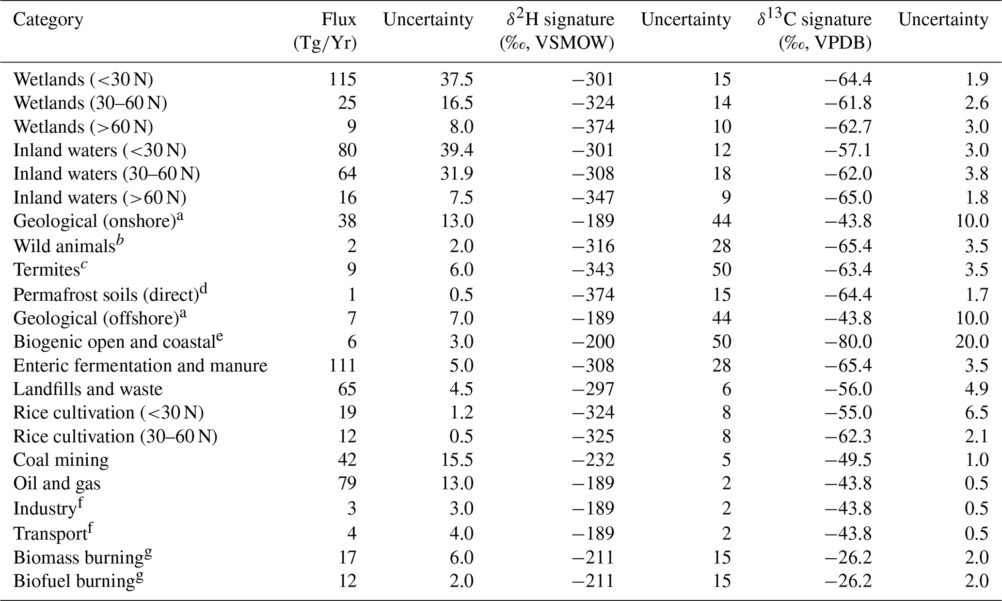
^a No specific isotopic measurements in the database (Sherwood et al., 2017). We applied the mean isotopic values for oil and gas and applied the standard deviation of for oil and gas as the uncertainty. ^b No specific isotopic measurements in database (Sherwood et al., 2017). We used the isotopic values and uncertainties from livestock. ^c Only one δ²H measurement in database (Sherwood et al., 2017). We applied 50 ‰ as a conservative uncertainty estimate. ^d No specific isotopic measurement in database (Sherwood et al., 2017). We used the isotopic values and uncertainties for high-latitude wetlands. ^e No specific isotopic measurements in database (Sherwood et al., 2017). We applied approximate isotopic values based on Whiticar (1999) and conservatively large uncertainty estimates. ^f No specific isotopic measurements in database (Sherwood et al., 2017). We used the isotopic values and uncertainties for oil and gas. ^g We applied all isotopic measurements of biomass burning to both the biomass burning and biofuel burning categories. We did not correct for the relative proportion of C₃ and C₄ plant combustion sources (see Sect. 2.4).

Download Print Version | Download XLSX

To calculate mean δ¹³C-CH₄ from wetlands, inland waters, and rice paddies for different latitudinal bands, we combined the data from this study along with additional data from Sherwood et al. (2017) (32 additional sites) to make our estimated source signatures as representative as possible. To our knowledge this combined dataset is the largest available compiled dataset of freshwater δ¹³C-CH₄ (see Sect. 2.3). Sites dominated by C₄ plants are notably underrepresented in this combined dataset. In addition, the biomass burning dataset of Sherwood e al. (2017) contains very few data from C₄ plant combustion. We performed a separate estimate of global source δ¹³C-CH₄ that attempted to correct for these likely biases by making two adjustments: (1) using the estimated low-latitude wetland δ¹³C-CH₄ signature of Ganesan et al. (2018) (−56.7 ‰), which takes into account the predicted spatial distribution of C₄-plant-dominated wetlands and (2) using the biomass burning δ¹³C-CH₄ signature of Schwietzke et al. (2016) (−22.3 ‰), which is weighted by the predicted contribution from C₄ plant combustion. We did not attempt to take into account δ¹³C-CH₄ from ruminants feeding on C₄ plants. For the C₄-plant-corrected δ¹³C-CH₄ estimate, we applied the same uncertainties that are reported in Table 1.

Since fluxes from other natural sources are not differentiated for the period 2008–2017, we calculated the proportional contribution of each category of other natural sources for the period 2000–2009 (Saunois et al., 2020), and we applied this to the total flux from other natural sources for 2008–2017. Inland waters and rice paddies do not have geographically resolved fluxes reported in Saunois et al. (2020). Therefore, we calculated the proportion of other natural sources attributed to inland waters from 2000–2009 (71 %), and we applied this proportion to the geographically resolved fluxes of other natural sources. Similarly, we calculated the proportion of agricultural and waste sources attributed to rice agriculture from 2008–2017 (15 %), and we applied this to the geographically resolved fluxes of agricultural and waste fluxes.

To estimate uncertainty in the modelled total source δ²H and δ¹³C values, we conducted Monte Carlo analyses (Thompson et al., 1992). We first estimated the uncertainty for each flux, δ²H, and δ¹³C term. Flux uncertainties were defined as one-half of the range of estimates provided by Saunois et al. (2020). For sources where fluxes were calculated as a proportion of a larger flux, we applied the same proportional calculation to uncertainty estimates. In cases where one-half of the range of reported studies was larger than the flux estimate, we set the uncertainty to be equal to the flux estimate to avoid negative fluxes in the mixing model. Isotopic source signal uncertainties were defined as the 95 % confidence interval of the mean value for a given source category. For some sources there are insufficient data to calculate a 95 % confidence interval, and we applied a conservative estimate of uncertainty for these sources, as detailed in Table 1. Confidence intervals for fossil fuel isotopic source signatures do not take into account variation in emissions fluxes and isotopic values between regions or resource types (i.e. conventional vs. unconventional reservoirs). This variation is difficult to quantify with available datasets but could imply additional uncertainty in global source signatures. We recalculated the δ²H and δ¹³C mixing models 10 000 times, each time sampling inputs from the uncertainty distribution for each variable. We assumed all uncertainties were normally distributed. We interpret the 2σ standard deviation of the resulting Monte Carlo distributions as an estimate of the uncertainty of our total atmospheric CH₄ source isotopic values. To examine how the Monte Carlo analyses were specifically influenced by uncertainty in isotopic source signatures vs. flux estimates, we conducted sensitivity tests where we set the uncertainty in either isotopic source signatures or flux estimates to zero. We also used the mixing model and Monte Carlo method to estimate the mean flux-weighted freshwater δ²H–CH₄ and δ¹³C-CH₄, using only the inputs for freshwater environments (wetlands, inland waters, and rice cultivation) from Table 1 (see Sect. 3.5).

3.1 Dataset distribution

The dataset is primarily concentrated in the Northern Hemisphere (Fig. 1a) but is distributed across a wide range of latitudes between 3^∘ S and 73^∘ N (Fig. 1c). The majority of sampled sites are from North America (Fig. 1b), but there are numerous sites from Eurasia. A much smaller number of sites are from South America and Africa. We define three latitudinal bands for describing geographic trends: low latitudes (3^∘ S to 30^∘ N), mid-latitudes (30 to 60^∘ N), and high-latitudes (60 to 90^∘ N). This definition was used primarily because it corresponds with a commonly applied geographic classification of CH₄ fluxes (Saunois et al., 2020).

Figure 1Distribution of sites shown (a) on a global map, with site mean CH₄-δ²H values indicated in relation to a colour bar. Sites with and without measured δ²H–H₂O are differentiated: (b) on a map of North America and (c) as a histogram of sites by latitude, differentiated between wetlands and inland waters. Dashed lines in (c) indicate divisions between low-latitude, mid-latitude, and high-latitude sites.

A total of 74 of 129 sites are classified as inland waters, primarily lakes (n=66), with a smaller number from rivers (n=8). To our knowledge, all of the inland water sites are natural ecosystems and do not include reservoirs. A total of 55 sites are classified as wetlands, including 16 bogs, 14 swamps and marshes, 12 fens, and 8 rice paddies. For the majority of sites (n=84) gas samples were measured, whereas studies at 36 sites measured dissolved CH₄ or diffusive fluxes.

3.2 Use of δ²H_p as an estimator for freshwater δ²H–H₂O

As discussed in Sect. 2.2.3, we regressed annual and growing season δ²H_p against measured δ²H–H₂O to determine which is a better estimator for sites where δ²H–H₂O is not measured. We performed this analysis separately for wetland and inland water environments because these broad environmental categories have distinct hydrological characteristics. For all regression analyses we found strong correlations, with R² values between 0.82 and 0.88 (Fig. 2). For wetlands, regression using annual δ²H_p produces a slightly better fit and also produces a slope within uncertainty of 1 (Fig. 2a), suggesting that variation in annual δ²H_p scales proportionately with variation in measured δ²H–H₂O. However, the intercept of this relationship was significantly greater than 0 (19 ± 9 ‰). We interpret this intercept as indicating that evaporative isotopic enrichment is generally important in controlling δ²H–H₂O in wetlands. A slope slightly greater than 1 is also consistent with evaporative enrichment, since greater evaporation rates would be expected in low-latitude environments with higher δ²H–H₂O. These results are consistent with detailed studies of wetland isotope hydrology that indicate a major contribution from groundwater, with highly dampened seasonal variability relative to precipitation, but also indicate evaporative enrichment of water isotopes in shallow soil water (Sprenger et al., 2017; David et al., 2018).

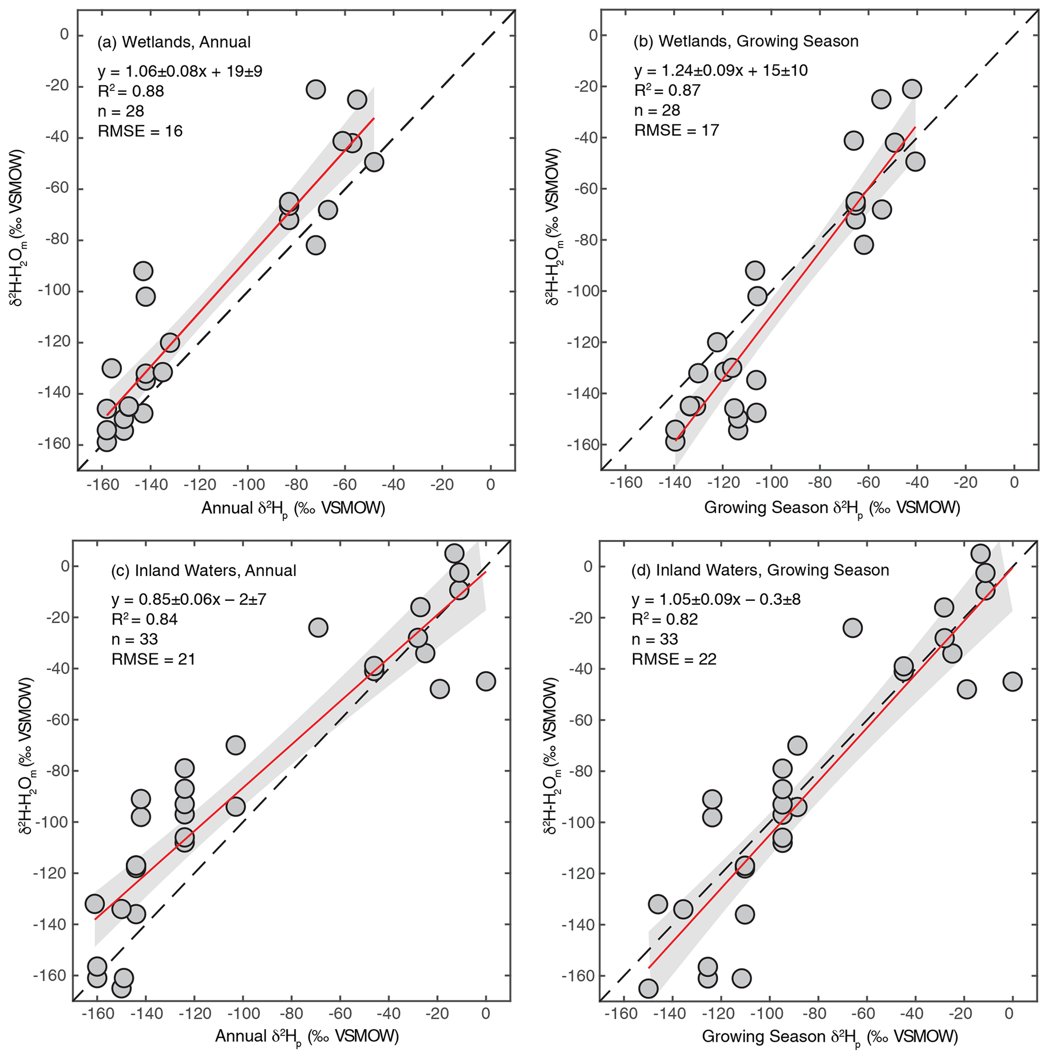
Figure 2Scatter plots of annual or growing season δ²H_p vs. measured δ²H–H₂O for wetland (a, b) and inland water (c, d) sites. The red lines indicate the best fit, with a 95 % confidence interval (grey envelopes), and the dashed black lines are the 1:1 relationship.

Download

For inland waters, regression with growing season δ²H_p produces a relationship that is within error of the 1:1 line (Fig. 2c), in contrast to annual δ²H_p, which produces a flatter slope (Fig. 2d). We infer that seasonal differences in δ²H_p are important in determining δ²H–H₂O in the inland water environments analyzed, especially at high latitudes, implying that these environments generally have water residence times on subannual timescales. This finding is generally consistent with evidence for seasonal variation in lake water isotopic compositions that is dependent on lake water residence times (Tyler et al., 2007; Jonsson et al., 2009). Lake water residence times vary widely, primarily as a function of lake size, but isotopic data imply that small lakes have water residence times of less than a year (Brooks et al., 2014), resulting in seasonal isotopic variability (Jonsson et al., 2009). Isotopic enrichment of lake water is highly variable but is typically minor in humid and high-latitude regions (Jonsson et al., 2009; Brooks et al., 2014), which characterizes most of our study sites.

Based on these results we combine measured and estimated δ²H–H₂O to determine a best-estimate value for each site, an approach similar to that of Waldron et al. (1999a). For sites with measured δ²H–H₂O values we use that value. For inland water sites without measured δ²H–H₂O we use modelled growing season δ²H_p since the regression of this against measured δ²H–H₂O is indistinguishable from the 1:1 line (Fig. 2d). For wetland sites without measured δ²H–H₂O, we estimate δ²H–H₂O using the regression relationship with annual precipitation δ²H–H₂O shown in Fig. 2a. The root-mean-square errors (RMSE) of these relationships (16 ‰ for wetlands, 22 ‰ for inland waters) provide an estimate of the uncertainty associated with estimating δ²H–H₂O using δ²H_p. Given the uncertainty associated with estimating δ²H–H₂O using δ²H_p, for all analyses presented below that depend on δ²H–H₂O values we also analyse the dataset only including sites with measured δ²H–H₂O.

3.3 Relationship between δ²H–H₂O and δ²H–CH₄

We carried out regression analyses of δ²H–H₂O vs. δ²H–CH₄, both using best-estimate δ²H–H₂O as described in Sect. 3.2 (Fig. 3a) and only including sites with measured δ²H–H₂O (Fig. 3b). In addition we analysed the relationship for all sites using annual (Fig. 3c) and growing season (Fig. 3d) δ²H_p. Identifying the relationship between modelled δ²H_p and δ²H–CH₄ is of value because this could be used to create gridded global predictions of δ²H–CH₄ based on gridded datasets of δ²H_p (Bowen and Revenaugh, 2003), as well as to predict the distribution of δ²H–CH₄ under past and future global climates using isotope enabled Earth system models (Zhu et al., 2017).

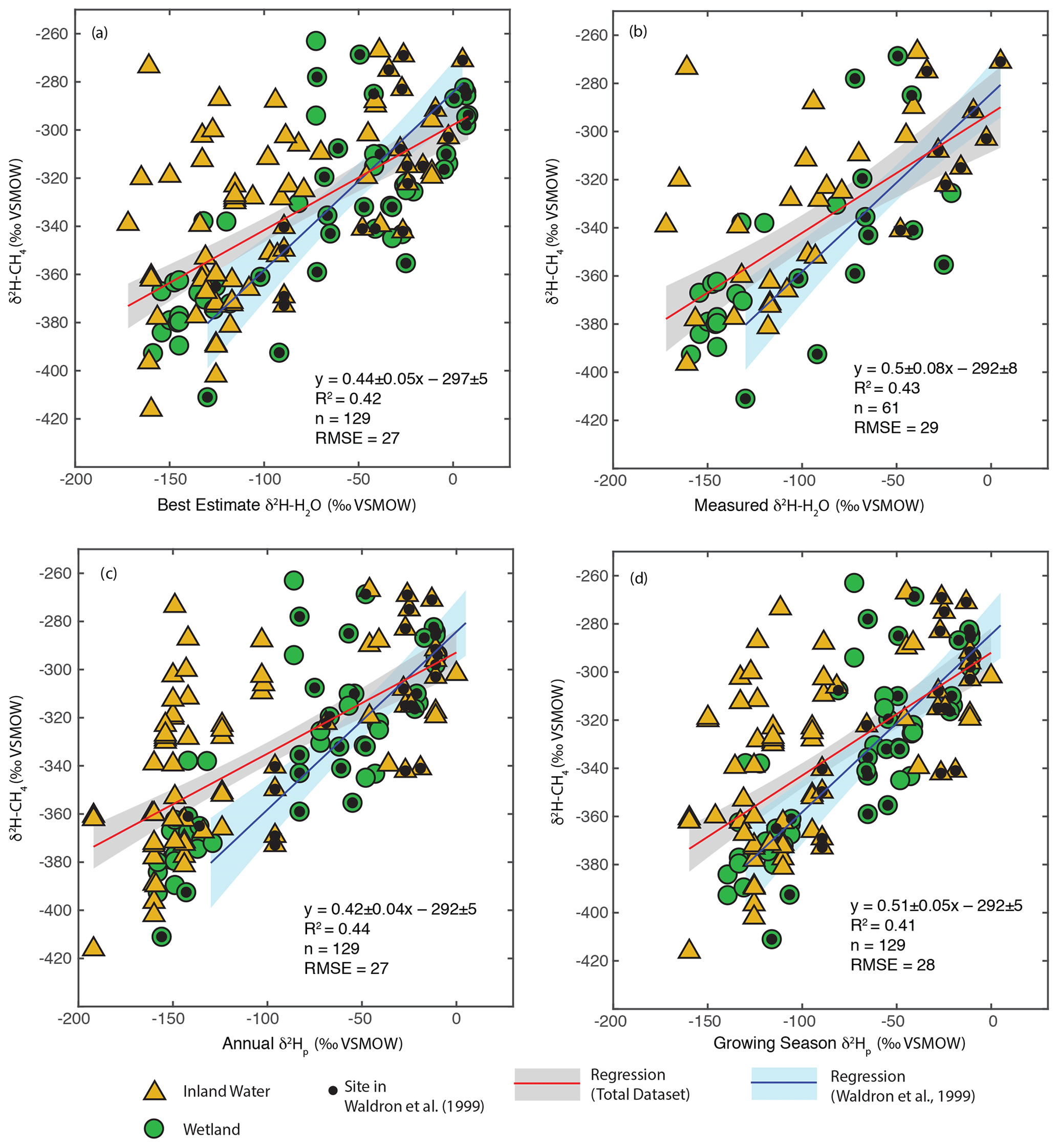
Figure 3Scatter plots of δ²H–CH₄ vs. (a) best-estimate δ²H–H₂O, (b) measured δ²H–H₂O, (c) annual δ²H_p, and (d) growing season δ²H_p. Sites that were included in the analysis of Waldron et al. (1999a) are indicated. The regression relationship for the total dataset in each plot is shown by the red line, with its 95 % confidence interval (grey envelope). The regression relationship and confidence interval for the dataset of Waldron et al. (1999a) are shown in blue. Uncertainties for reported regression relationships are standard errors.

Download

δ²H–CH₄ is significantly positively correlated with δ²H–H₂O when using all four methods of estimating δ²H–H₂O (Fig. 3, Supplement Table S2). This is the case when analysing all sites together, as well as when analysing wetlands and inland waters separately (Douglas et al., 2020b, Supplement Table S2, Fig. 4). There is no significant difference in regression relationships, based on analysis of covariance, when δ²H–CH₄ is regressed against best-estimate δ²H–H₂O, measured δ²H–H₂O, or modelled δ²H_p, nor is there a major difference in R² values or RMSE (Douglas et al., 2020b, Supplement Table S2). Regression with wetland sites consistently results in a higher R² values and lower RMSE than regression with inland water sites.

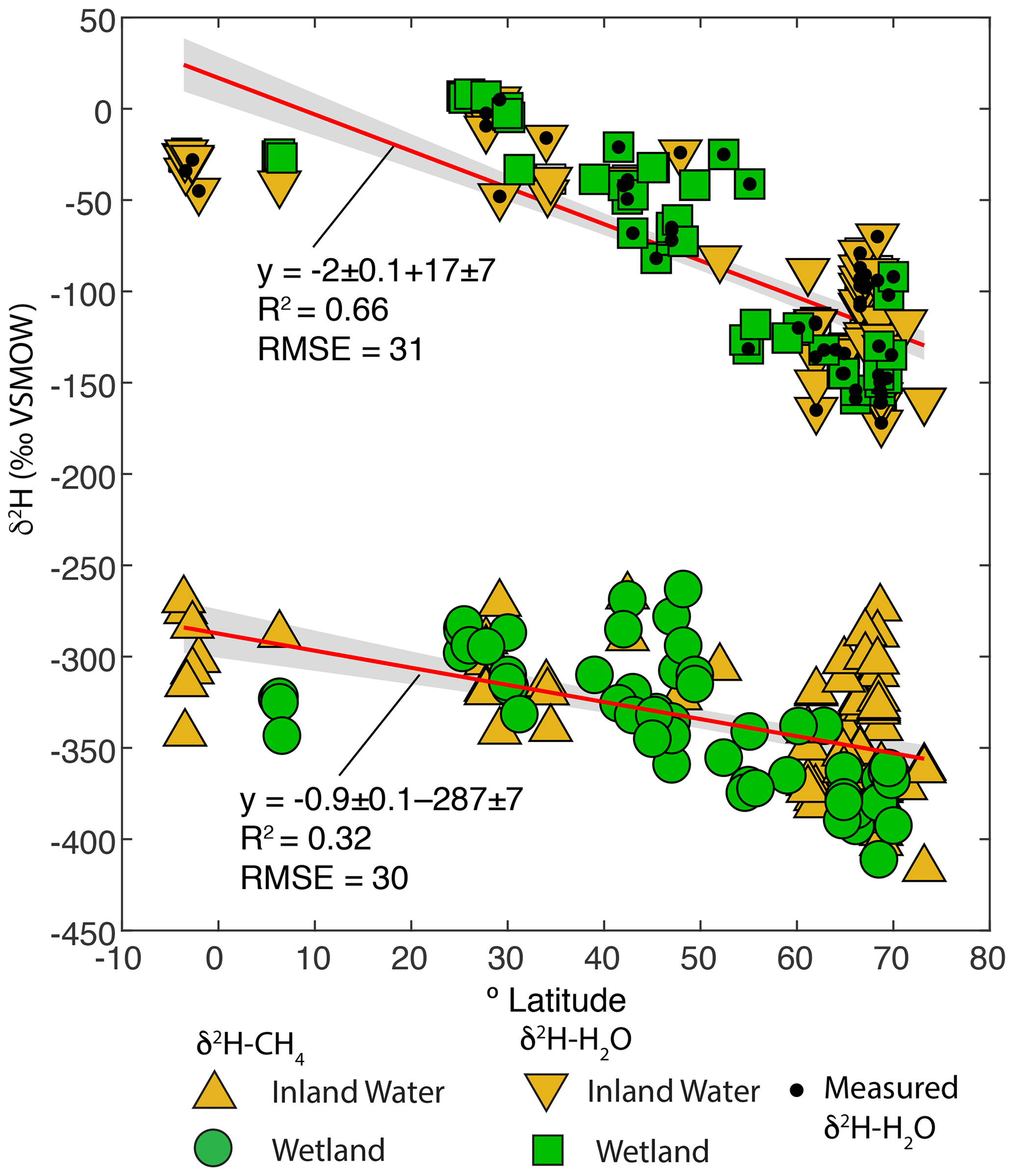
Figure 4Scatter plots of δ²H–CH₄ and best-estimate δ²H–H₂O, vs. latitude (^∘ N). Sites with measured δ²H–H₂O are indicated. Envelopes indicate 95 % confidence intervals for regression lines.

Download

Given the similar results when regressing with estimated or measured δ²H–H₂O, we infer that using either the “best-estimate” δ²H–H₂O or modelled δ²H_p, instead of measured δ²H–H₂O, to predict δ²H–CH₄ does not result in substantial additional error. This implies that isotope-enabled Earth system models (ESMs) could be used to predict the distribution of freshwater δ²H–CH₄ under past and future climates based on modelled δ²H_p, although the substantial scatter in Fig. 3c and d should be taken into account. The Southern Hemisphere is highly underrepresented in the δ²H–CH₄ dataset. However, the mechanisms linking δ²H–CH₄ with δ²H–H₂O should not differ in the Southern Hemisphere, and we argue that the relationships observed in this study are suitable to predict Southern Hemisphere freshwater δ²H–CH₄. The choice of predicting δ²H–CH₄ using growing-season vs. annual precipitation δ²H_p could be important, with steeper slopes overall when regressing against growing season δ²H_p. Based on our analysis in Sect. 3.2, we suggest that annual δ²H_p may be more appropriate for estimating wetland δ²H–CH₄, while growing season δ²H_p may be more appropriate for estimating inland water δ²H–CH₄. Forthcoming research will combine gridded datasets of wetland distribution (Ganesan et al., 2018), modelled annual δ²H_p (Bowen and Revenaugh, 2003), and the regression relationships from this study to predict spatially resolved wetland δ²H–CH₄ at a global scale (Stell et al., 2021).

Overall, our results are broadly consistent with those of Waldron et al. (1999a), and confirm the finding of that study that δ²H–H₂O is the predominant predictor of global variation in δ²H–CH₄. All of the regression slopes produced using our dataset are flatter than the regression relationship found by Waldron et al. (1999a) using a smaller dataset (0.68 ± 0.1), although the slopes are not significantly different based on analysis of covariance. Based on this result we infer that the true global relationship is likely flatter than that estimated by Waldron et al. (1999a). The difference between the regression relationships reported here and that of Waldron et al. (1999a) is largely a result of a much greater number of samples from the high latitudes (Fig. 1c), where δ²H–H₂O values are typically lower. The small number of high-latitude sites sampled by Waldron et al. (1999a) are skewed towards the low end of the high-latitude δ²H–CH₄ data from this study (Fig. 3). A similarly flatter slope (0.54 ± 0.05) was found by Chanton et al. (2006) when combining a dataset of δ²H–CH₄ from Alaskan wetlands, which are included in this study, with the dataset of Waldron et al. (1999a). Based on the range of R² values shown in Fig. 3, we estimate that δ²H–H₂O explains approximately 42 % of variability in δ²H–CH₄, implying substantial residual variability, with greater residual variability for inland water sites than for wetlands (Douglas et al., 2020b, Supplement Table S2).

Given that δ²H–H₂O is strongly influenced by latitude we examined whether δ²H–CH₄ is also significantly correlated with latitude. There is indeed a significant negative relationship between latitude and δ²H–CH₄, indicating an approximate decrease of 0.9 ‰ per degree latitude (Fig. 4). The slope is significantly flatter than that for latitude vs. δ²H–H₂O in this dataset (−2 ‰ per degree latitude), which is consistent with the inferred slope for δ²H–H₂O vs. δ²H–CH₄ (0.44 to 0.5). There is greater scatter in δ²H–CH₄ at higher latitudes, especially for inland waters, but it is unclear whether this is simply a result of a larger sample set or of differences in the underlying processes controlling δ²H–CH₄. We discuss latitudinal differences in δ²H–CH₄ in further detail in Sect. 3.5.

Comparison of δ²H–H₂O vs. δ²H–CH₄ relationships between environmental and experimental studies

To further understand the processes controlling the observed freshwater δ²H–H₂O vs. δ²H–CH₄ relationships, we compared them to results from pure culture and incubation experiments across a wide range of δ²H–H₂O values (Fig. 5), focusing on regression against best-estimate δ²H–H₂O. The regression slopes for both wetlands and inland waters (0.5 and 0.42) are within error of the in vitro relationship compiled by Waldron et al. (1999a) (0.44), based on laboratory incubations from three separate studies (Schoell, 1980; Sugimoto and Wada, 1995; Waldron et al., 1998). The intercept for the wetland and inland water regressions is higher than that for the in vitro relationship, although only the difference with inland waters is significant. In contrast, the regression slope for pure-culture acetoclastic methanogenesis experiments is much flatter (0.18 to 0.2) (Valentine et al., 2004b; Gruen et al., 2018), consistent with the prediction that one hydrogen atom is exchanged between water and the acetate methyl group during CH₄ formation (Pine and Barker, 1956; Whiticar, 1999). The large difference in intercept between the two acetate pure culture datasets is likely a function of differences in the δ²H of acetate between the experiments but could also be influenced by differences in kinetic isotope effects (Valentine et al., 2004b).

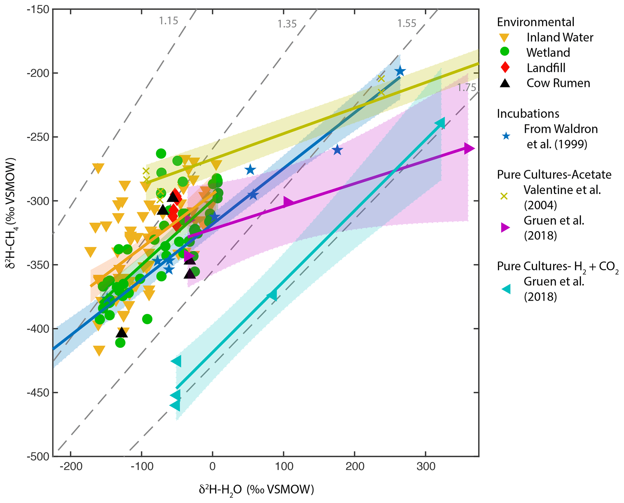
Figure 5Scatter plots of δ²H–CH₄ vs. δ²H–H₂O for wetlands, inland waters, landfills, and cow rumen, compared with incubation and pure-culture experiments. Regression lines and confidence intervals corresponding to each dataset (except landfills and cow rumen) are shown. Dashed grey lines indicate constant values of α_H. Regression line statistics are listed in Supplement Table S2. Plotted δ²H–H₂O values are best-estimate values for wetlands and inland waters, measured values for culture experiments, and a combination of measured values and annual δ²H_p for landfills and cow rumen (see Supplement Table S3 for more details, Douglas et al., 2020b).

Download

Pure-culture hydrogenotrophic methanogenesis experiments (Gruen et al., 2018) yield a regression slope that is consistent with a constant α_H value, although α_H can clearly vary depending on experimental or environmental conditions (Valentine et al., 2004b; Stolper et al., 2015; Douglas et al., 2016). The wetland, inland water, and in vitro regression relationships are not consistent with a constant value of α_H (Fig. 5). Our comparison supports previous inferences that the in vitro line of Waldron et al. (1999a) provides a good estimate of the slope of environmental δ²H–H₂O vs. δ²H–CH₄ relationships. This slope is likely controlled by the relative proportion of acetoclastic and hydrogenotrophic methanogenesis, the net kinetic isotope effect associated with these two methanogenic pathways, and variance in δ²H of acetate (Waldron et al., 1998, 1999a; Valentine et al., 2004a), but the relative importance of these variables remains uncertain.

In particular, the δ²H of acetate methyl hydrogen is probably influenced by environmental δ²H–H₂O and therefore likely varies geographically as a function of δ²H_p, as originally hypothesized by Waldron et al. (1999a). To our knowledge there are no measurements of acetate or acetate-methyl δ²H from natural environments with which to test this hypothesis. In general, variability in the δ²H of environmental organic molecules in lake sediments and wetlands, including fatty acids and cellulose, is largely controlled by δ²H–H₂O (Huang et al., 2002; Sachse et al., 2012; Mora and Zanazzi, 2017), albeit with widely varying fractionation factors. The δ²H of methoxyl groups in plants has also been shown to vary as a function of δ²H–H₂O (Vigano et al., 2010). Furthermore, culture experiments with acetogenic bacteria imply that there is rapid isotopic exchange between H₂ and H₂O during chemoautotrophic acetogenesis (Valentine et al., 2004a), implying that the δ²H of chemoautotrophic acetate is also partially controlled by environmental δ²H–H₂O. Incubation experiments, such as those included in the in vitro line (Schoell, 1980; Sugimoto and Wada, 1995; Waldron et al., 1998), probably contain acetate-δ²H that varies as a function of ambient δ²H–H₂O, given that the acetate in these incubation experiments was actively produced by fermentation and/or acetogenesis during the course of the experiment. This differs from pure cultures of methanogens, where acetate is provided in the culture medium and therefore does not vary in its δ²H value (Valentine et al., 2004b; Gruen et al., 2018).

3.4 Relationship of δ²H–CH₄ with δ¹³C-CH₄, δ¹³C–CO₂, and α_C

As shown in Fig. 3, there is a large amount of residual variability in δ²H–CH₄ that is not explained by δ²H–H₂O. Several biogeochemical variables have been proposed to influence freshwater δ²H–CH₄ independently of δ²H–H₂O, including the predominant biochemical pathway of methanogenesis (Whiticar et al., 1986; Whiticar, 1999; Chanton et al., 2006), the extent of methane oxidation (Happell et al., 1994; Waldron et al., 1999a; Whiticar, 1999; Cadieux et al., 2016), isotopic fractionation resulting from diffusive gas transport (Waldron et al., 1999a; Chanton, 2005), and differences in the thermodynamic favorability or reversibility of methanogenesis (Valentine et al., 2004b; Stolper et al., 2015; Douglas et al., 2016). These variables are also predicted to cause differences in δ¹³C-CH₄, δ¹³C–CO₂, and α_C. Therefore, we analysed co-variation between δ²H–CH_4,W0 (see definition in Sect. 2.2.3) and δ¹³C-CH₄, δ¹³C–CO₂, and α_C to see whether it could partially explain the residual variability in δ²H–CH₄ (Fig. 6).

In order to facilitate interpretation of isotopic co-variation, we estimated approximate vectors of predicted isotopic co-variation for the four variables being considered (Fig. 6). We emphasize that these vectors are uncertain, and while they can be considered indicators for the sign of the slope of co-variation and the relative magnitude of expected isotopic variability, they are not precise representations of the slope or intercept of isotopic co-variation. In reality, isotopic co-variance associated with these processes likely varies depending on specific environmental conditions, although the sign of co-variance should be consistent. The starting point for the vectors is arbitrarily set to typical isotopic values for inferred acetoclastic methanogenesis in freshwater systems (Whiticar, 1999). We based the vectors for differences in the dominant methanogenic pathway and methane oxidation in Figs. 8, 5, and 10 in Whiticar (1999). These figures are widely applied to interpret environmental isotopic data related to CH₄ cycling. However, we note that both environmental and experimental research has questioned whether differences in the dominant methanogenic pathway have an influence on δ²H–CH₄ (Waldron et al., 1998, 1999a). Differences in δ²H–CH₄ between hydrogenotrophic and acetoclastic methanogenesis are likely highly dependent on both the δ²H of acetate and the carbon and hydrogen kinetic isotope effects for both methanogenic pathways, both of which are poorly constrained in natural environments and are likely to vary between sites (see Sect. 3.3). We did not differentiate between anaerobic and aerobic methane oxidation, and the vectors shown are similar to experimental results for aerobic methane oxidation (Wang et al., 2016).

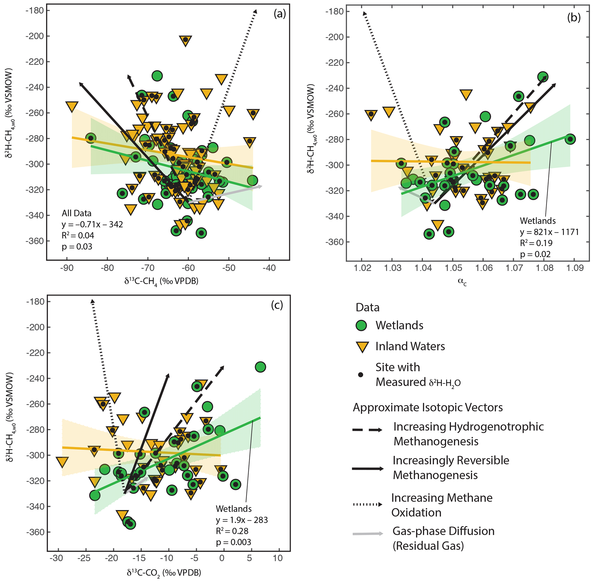
Figure 6Scatter plots of δ²H–CH_4,w0 vs. (a) δ¹³C-CH₄, (b) α_c, and (c) δ¹³C–CO₂. Approximate vectors for isotopic co-variation related to four biogeochemical variables are shown. See details in Sect. 3.4 and the Supplement. Regression relationships are shown for wetland and inland water sites, with envelopes indicating 95 % confidence intervals. Regression statistics are shown here for relationships with significant correlations (p<0.05). All regression statistics are detailed in Supplement Table S4 (Douglas et al., 2020b).

Download

The vector for isotopic fractionation related to gas-phase diffusion is based on the calculations of Chanton (2005) and indicates isotopic change for residual gas following a diffusive loss. Gas–liquid diffusion is predicted to have a much smaller isotopic effect (Chanton, 2005). The vector for differences in enzymatic reversibility is based on experiments where CH₄ and CO₂ isotopic compositions were measured together with changes in methane production rate or Gibbs free energy (Valentine et al., 2004b; Penning et al., 2005). We note that these studies did not measure δ²H–CH₄ in the same experiments as δ¹³C-CH₄ or δ¹³C–CO₂, implying large uncertainty in the co-variance vectors. More detail on the estimated vectors is provided in the Supplement.

We observe significant positive correlations between δ²H–CH_4,W0, calculated using best estimate δ²H–H₂O, and both δ¹³C–CO₂ and α_C for wetland sites (Douglas et al., 2020b, Fig. 6b, c; Supplement Table S4). We do not observe a significant correlation between these variables for inland water sites or for the dataset as a whole. We also observe a weak but significant negative correlation between δ²H–CH_4,W0 and δ¹³C-CH₄ for all sites but not for data disaggregated into wetlands and inland water categories (Fig. 6a). The correlations shown in Fig. 6 should be interpreted with caution, since repeating this analysis only using sites with measured δ²H–H₂O does not result in any significant correlations (Douglas et al., 2020b, Supplement Table S4). It is unclear whether this different result when using best-estimate or measured δ²H–H₂O represents a bias related to estimating δ²H–H₂O using δ²H_p or is an effect of the much smaller sample size for sites with δ²H–H₂O measurements. If accurate, the observed significant positive correlations in Fig. 6b and c suggest that residual variability in δ²H–CH₄ in wetlands is more strongly controlled by biogeochemical variables related to methanogenesis, namely differences in methanogenic pathway or thermodynamic favorability, than post-production processes such as diffusive transport and CH₄ oxidation. For inland water sites our analysis suggests that no single biogeochemical variable has a clear effect in controlling residual variability in δ²H–CH₄.

Overall, our results are not consistent with arguments that residual variability in freshwater δ²H–CH₄ is dominantly controlled by either differences in methanogenic pathway (Chanton et al., 2006) or post-production processes (Waldron et al., 1999a). Instead they highlight the combined influence of a complex set of variables and processes that are difficult to disentangle on an inter-site basis using δ¹³C measurements alone. It is also important to note the likely importance of variables that could influence δ¹³C-CH₄ or δ¹³C–CO₂ but not necessarily affect δ²H–CH₄, including variance in the δ¹³C of soil or sediment organic matter (Conrad et al., 2011; Ganesan et al., 2018), diverse metabolic and environmental sources and sinks of CO₂ in aquatic environments, and Rayleigh fractionation associated with CH₄ carbon substrate depletion (Whiticar, 1999). Finally, the possible role of other carbon substrates, such as methanol, in CH₄ production could be important in controlling isotopic co-variation. Culture experiments suggest that CH₄ produced from methanol has low δ¹³C and δ²H values relative to other pathways (Krzycki et al., 1987; Penger et al., 2012; Gruen et al., 2018), although the importance of this difference in environmental CH₄ is unclear.

Further research examining intra-site isotopic co-variation, which largely avoids complications associated with estimating δ²H–H₂O, would help to more clearly resolve the relative importance of these processes and how they vary between environments. Expanded research using methyl fluoride to inhibit acetoclastic methanogenesis (Penning et al., 2005; Penning and Conrad, 2007; Conrad et al., 2011), with a particular focus on δ²H–CH₄ measurements, would also help to clarify the importance of methanogenic pathway on isotopic co-variation. Finally, an expanded application of measurements of clumped isotopes, which have distinctive patterns of variation related to these processes (Douglas et al., 2016, 2017; Young et al., 2017; Douglas et al., 2020a), would also be of value in determining their relative importance in controlling δ²H–CH₄ values in freshwater environments.

3.5 Differences in δ²H–CH₄ and δ¹³C-CH₄ by latitude

When analysing all sites together, we found a significant difference in the distribution of δ²H–CH₄ between high-latitude sites (median: −351 ‰) and both low- (median: −298 ‰) and mid-latitude sites (median: −320 ‰) (Fig. 7a). However, we did not find a significant difference in the distribution of low- and mid-latitude sites. Similar differences were found when the data were disaggregated into wetland and inland water sites. We also found that the distribution of δ¹³C-CH₄ for low-latitude sites (median: −61.6 ‰) was significantly higher than for high-latitude sites (median: −63.0 ‰) but that mid-latitude sites (median: −60.3 ‰) were not significantly different from the other two latitudinal zones (Fig. 7b). The observed difference by latitudinal zone in δ¹³C-CH₄ appears to be driven primarily by latitudinal differences between inland water sites, where a similar pattern is found. In wetland sites we found no significant differences in the distribution of δ¹³C-CH₄ by latitude.

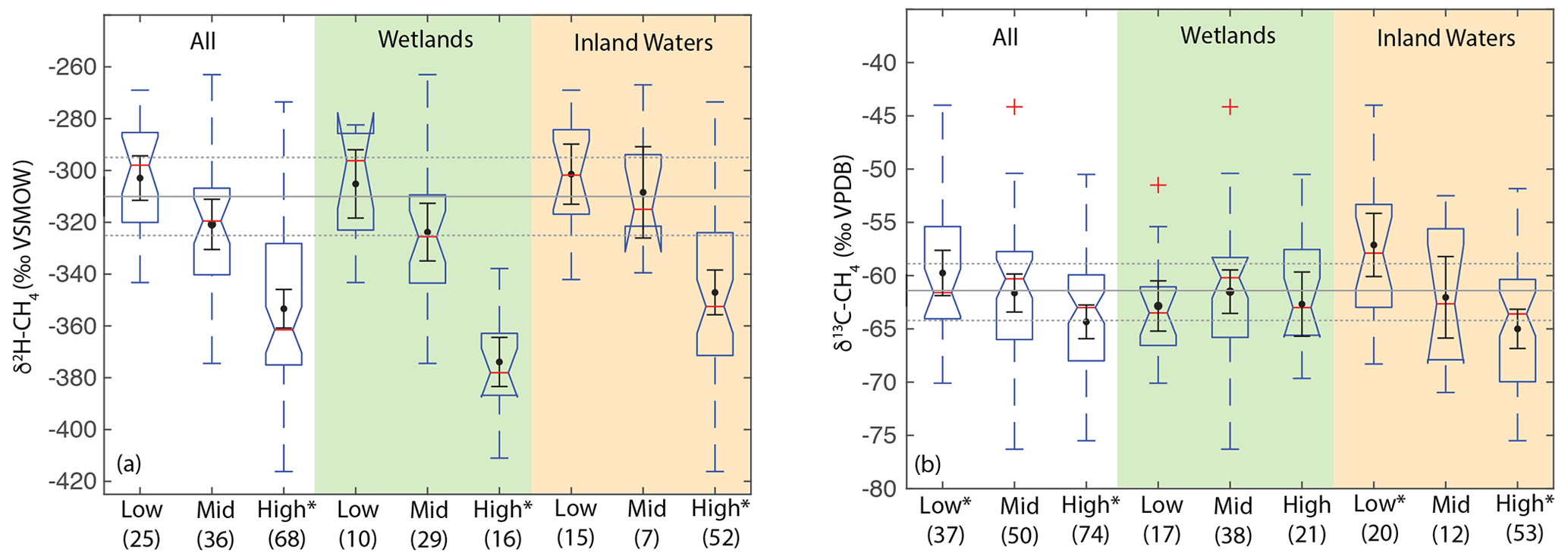
Figure 7Boxplots of (a) δ²H–CH₄ and (b) δ¹³C-CH₄ for sites differentiated by latitude, for all data, wetlands, and inland waters. Numbers in parentheses indicate the number of sites for each category. Red lines indicate medians, boxes indicate 25th and 75th percentiles, whiskers indicate 95th and 5th percentiles, and outliers are shown as red crosses. Notches indicate the 95 % confidence intervals of the median value; where notches overlap the edges of the box this indicates the median confidence interval exceeds the 75th or 25th percentile. Black points and error bars indicate the category mean and 95 % confidence interval of the mean. Grey lines indicate the estimated flux-weighted mean values for global freshwater CH₄, and dashed lines indicate the 95 % confidence interval of this value. Asterisks in (a) indicate that high-latitude sites have significantly different distributions from other latitudinal bands. Asterisks in (b) indicate groups that have significantly different distributions from one another, within a specific environmental category. Two extremely low outliers (<−80 ‰; high-latitude wetland and inland water) are not shown in (b).

Download

Estimates of flux-weighted mean freshwater δ²H–CH₄ and δ¹³C-CH₄, calculated using the Monte Carlo approach described in Sect. 2.4, are −310 ± 15 ‰ (Fig. 7a) and −61.5 ± 3 ‰ (Fig. 7b) respectively. Flux-weighted mean values for natural wetlands (not including inland waters or rice paddies) are −310 ± 25 ‰ for δ²H–CH₄ and −63.9 ± 3.3 ‰ for δ¹³C-CH₄. Flux-weighted mean values for inland waters are −309 ± 31 ‰ for δ²H–CH₄ and −60 ± 5.7 ‰ for δ¹³C-CH₄. As discussed in Sect. 2.4 there are limited data in our dataset or that of Sherwood et al. (2017) from C₄-plant-dominated wetlands, and therefore our low-latitude and flux-weighted mean δ¹³C-CH₄ values for wetlands are probably biased towards low values.

Differences in δ²H–CH₄ by latitude have the potential to aid in geographic discrimination of freshwater methane sources, both because it is based on a clear mechanistic linkage with δ²H–H₂O (Figs. 3 and 4) and because geographic variation in δ²H–H₂O is relatively well understood (Bowen and Revenaugh, 2003; Bowen et al., 2005). However, recent studies of atmospheric δ²H–CH₄ variation have typically not accounted for geographic variation in source signals. As an example, Rice et al. (2016) apply a constant δ²H–CH₄ of −322 ‰ for both low-latitude (0–30^∘ N) and high-latitude (30–90^∘ N) wetland emissions. Based on our dataset this estimate is an inaccurate representation of wetland δ²H–CH₄ for either 0–30^∘ N (mean: −305 ± 13 ‰) or 30–90^∘ N (mean: −345 ± 11 ‰). Studies of ice core measurements have more frequently differentiated freshwater δ²H–CH₄ values as a function of latitude. For example, Bock et al., (2010) differentiated δ²H–CH₄ between tropical (−320 ‰) and boreal (−370 ‰) wetlands. This tropical wetland signature is significantly lower than our estimate of low-latitude wetland δ²H–CH₄, although the boreal wetland signature is similar to our mean value for high-latitude wetlands (−374 ± 10 ‰). Overall, our results imply that accounting for latitudinal variation in freshwater δ²H–CH₄, along with accurate latitudinal flux estimates, is important for developing accurate estimates of global freshwater δ²H–CH₄ source signatures.

Our analysis indicates significant differences in the distribution of freshwater δ¹³C-CH₄ between the low- and high-latitudes, but mid-latitude sites cannot be differentiated. Furthermore our results do not indicate significant latitudinal differences in δ¹³C-CH₄ for wetland sites in particular. This is in contrast to previous studies that have inferred significant differences in wetland δ¹³C-CH₄ by latitude (Bock et al., 2010; Rice et al., 2016; Ganesan et al., 2018). An important caveat is that we have not analyzed a comprehensive dataset of freshwater δ¹³C-CH₄, for which there are much more published data than for δ²H–CH₄, although our analysis does comprise the largest dataset of freshwater δ¹³C-CH₄ compiled to date (see Sect. 2.3). In addition, our analysis does not take into account the geographic distribution of different ecosystem categories, although we do not find significant differences in δ¹³C-CH₄ between ecosystem categories (Fig. 8; Sect. 3.6). Low-latitude ecosystems dominated by C₄ plants are underrepresented in both our dataset and that of Sherwood et al. (2017), and accounting for this would likely lead to a more enriched low-latitude wetland δ¹³C-CH₄. In contrast, high-latitude ecosystems, including bogs, are relatively well represented in these datasets (Fig. 8), and we suggest that inferences of especially low δ¹³C-CH₄ in high-latitude wetlands (Bock et al., 2010; Rice et al., 2016; Ganesan et al., 2018) are not consistent with the compiled dataset of in situ measurements. However, we note that atmospheric estimates of high-latitude wetland δ¹³C-CH₄ (∼ −68 ± 4 ‰; Fisher et al., 2011) are lower than the median or mean value shown in Fig. 7b and are in close agreement with the relatively low values predicted by Ganesan et al. (2018). Ombrotrophic and minerotrophic peatlands have distinctive δ¹³C-CH₄ signatures (Bellisario et al., 1999; Bowes and Hornibrook, 2006; Hornibrook, 2009), with lower signatures in ombrotrophic peatlands. We did not differentiate peatlands by trophic status, and it is possible that the dataset of high-latitude wetland in situ measurements is biased towards minerotrophic peatlands with relatively high δ¹³C-CH₄.

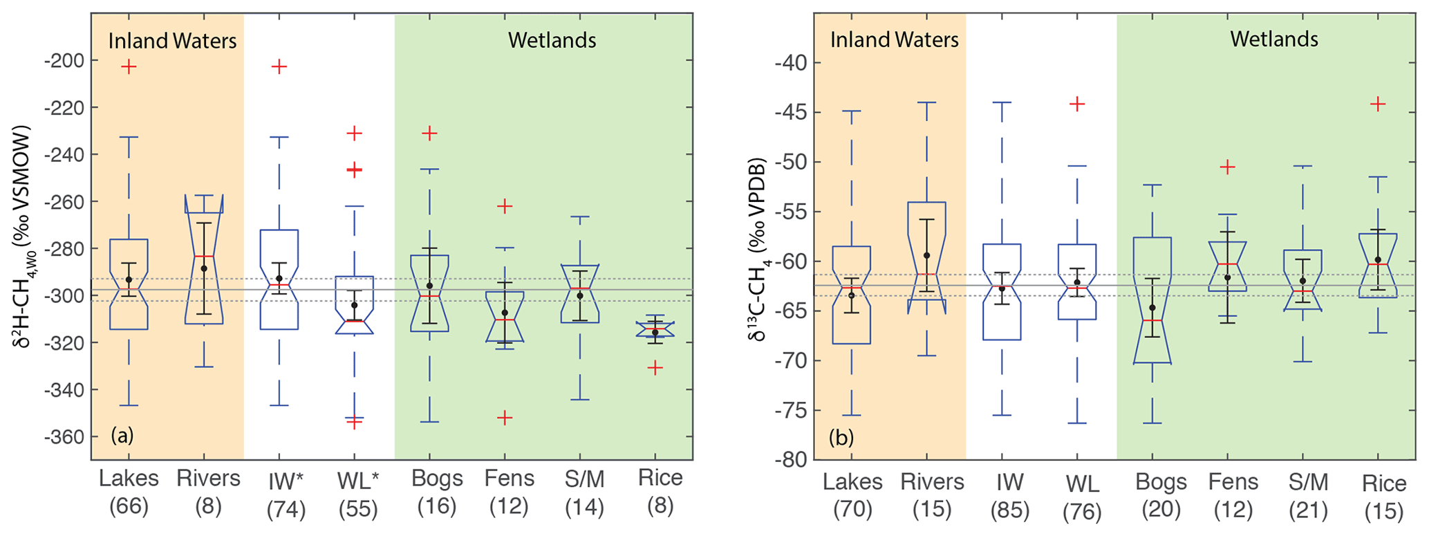
Figure 8Boxplots of (a) δ²H–CH_4,W0 and (b) δ¹³C-CH₄ for sites differentiated by ecosystem type. Numbers in parentheses indicate the number of sites for each category. Boxplot parameters are as in Fig. 7. Black points and error bars indicate the category mean and 95 % confidence interval of the mean. Grey lines indicate the mean values across all categories, and the dashed lines indicate the 95 % confidence interval of this value. Two extremely low outliers (<−80 ‰; lake and fen) are not shown in (b). IW – inland waters; WL – wetlands; S/M – swamps and marshes. Asterisks in A indicate that inland waters and wetlands have significantly different distributions.

Download

Latitudinal differences in δ¹³C-CH₄ inferred by Ganesan et al. (2018) were based on two key mechanisms: (1) differences in methanogenic pathway between different types of wetlands, especially between minerotrophic fens and ombrotrophic bogs; and (2) differential inputs of organic matter from C₃ and C₄ plants. Because inferred latitudinal differences in δ¹³C-CH₄ and δ²H–CH₄ are caused by different mechanisms, they could be highly complementary in validating estimates of freshwater emissions by latitude. It is also important to note that previous assessments of latitudinal differences in δ¹³C-CH₄ did not include inland water environments. Our analysis suggests that latitudinal variation in δ¹³C-CH₄ in inland waters may be more pronounced than in wetlands, although the mechanisms causing this difference will need to be elucidated with further study. A benefit of geographic discrimination based on δ²H–CH₄ is that the same causal mechanism applies to all freshwater emissions, including both wetlands and inland waters.

3.6 Differences in δ²H–CH₄ and δ¹³C-CH₄ by ecosystem

When comparing ecosystems, we analyze δ²H–CH_4,W0 values to account for variability related to differences in δ²H–H₂O. Ecosystem types are not evenly distributed by latitude and therefore have different distributions of δ²H–H₂O values. Our analysis does not find a significant difference in the distribution of δ²H–CH_4,W0 between ecosystems, which could be partly a result of small sample sizes for most ecosystem categories (Fig. 8). Comparing the broader categories of inland waters and wetlands, we do observe a significant difference in δ²H–CH_4,W0 distributions, with inland waters shifted towards higher values (median: −296 ‰) than wetlands (median: −311 ‰). We repeated this analysis only including sites with measured δ²H–H₂O and found the same results in terms of category differences (Supplement Fig. S1). We did not observe any significant differences in δ¹³C-CH₄ distributions between ecosystems, nor was there a significant difference in δ¹³C-CH₄ distributions between inland waters and wetlands.

The significant difference in the distribution of δ²H–CH_4,W0 between inland waters and wetlands is primarily a result of the difference in δ²H–CH₄ between these environments in the high latitudes (Figs. 3, 4, and 7). We suggest this difference could be related to a greater overall prevalence of CH₄ oxidation in inland waters. As shown in Fig. 6, the lack of positive co-variation between δ²H–CH_4,W0 and δ¹³C–CO₂ and α_C could be interpreted to support a greater role for CH₄ oxidation in controlling δ²H–CH_4,W0 in inland waters relative to wetlands, although this result requires further validation. In lakes that undergo seasonal overturning and water column oxygenation, there may be a greater overall effect of CH₄ oxidation than there is in wetlands typically. The absence of significant differences between ecosystems in terms of δ¹³C-CH₄ (Fig. 8b) is in contrast to previous studies that have suggested that fens and bogs in particular have distinctive δ¹³C-CH₄ (Ganesan et al., 2018). Bogs in particular have a very wide distribution of δ¹³C-CH₄ that could represent differences between minerotrophic and ombrotrophic bogs (Hornibrook, 2009), which we did not differentiate in our dataset. This result should be interpreted with caution given that our dataset is not a comprehensive compilation of published δ¹³C-CH₄ data, although it is the largest compiled dataset available (Sect. 2.3). We argue that inferred differences in δ¹³C-CH₄ between wetland ecosystem categories should be further verified with more comprehensive data assimilation and additional measurements.

3.7 Differences in δ²H–CH₄ and δ¹³C-CH₄ by sample type

As with comparing ecosystems, when comparing sample types we analyze δ²H–CH_4,W0 values to normalize for variability related to differences in δ²H–H₂O, since sample types are not distributed evenly by latitude. When comparing sample types, dissolved CH₄ samples do not have a significantly different δ²H–CH_4,W0 distribution for the dataset as a whole, nor is there a significant difference between these groups in wetland sites (Fig. 9a). There is, however, a significant difference in inland water sites, with dissolved CH₄ samples having a more enriched distribution (median: −270 ‰) vs. gas samples (median: −302 ‰). We repeated this analysis only including sites with measured δ²H–H₂O and found the same results in terms of category differences (Supplement Fig. S2). We did not observe a significant difference in the distribution of δ¹³C between dissolved and gas-phase CH₄ samples, either for the dataset as a whole or when the dataset was disaggregated into wetlands and inland waters (Fig. 9b).

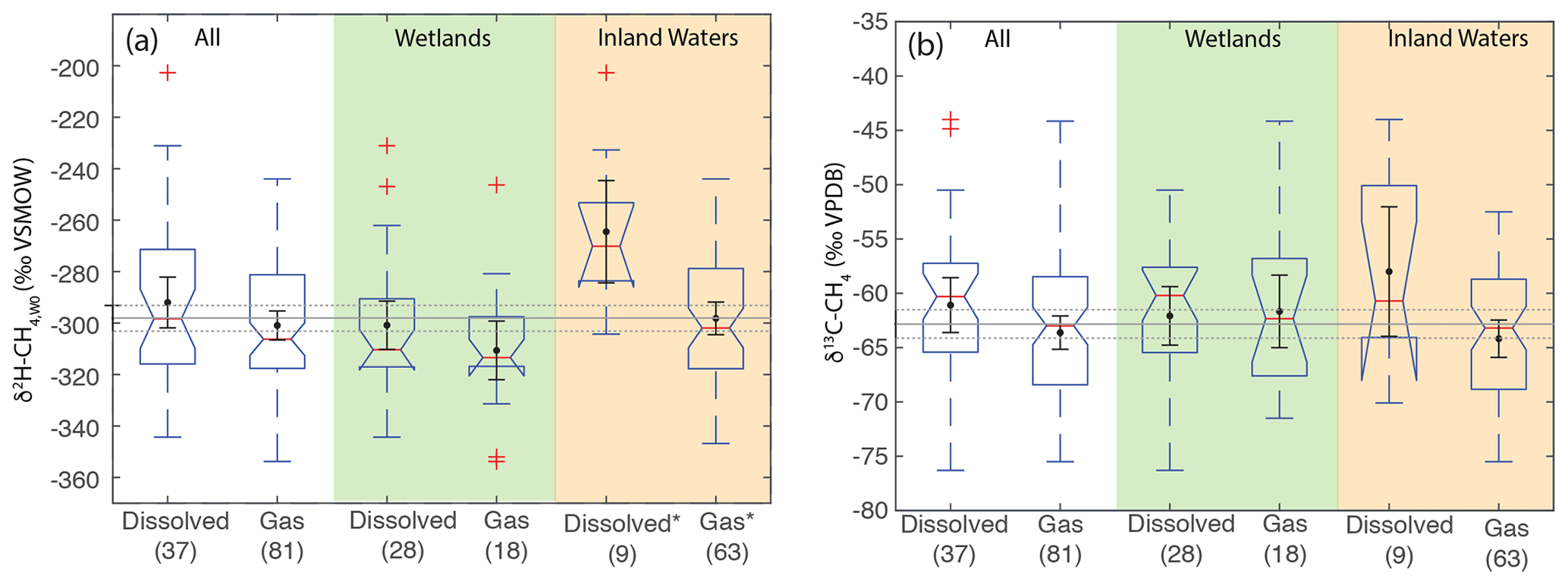
Figure 9Boxplots of (a) δ²H–CH_4,W0 and (b) δ¹³C-CH₄ for sites differentiated by sample type. Numbers in parentheses indicate the number of sites for each category. Boxplot parameters are as in Fig. 7. Black points and error bars indicate the category mean and 95 % confidence interval of the mean. Grey lines indicate the mean values across all categories, and the dashed lines indicate the 95 % confidence interval of this value. Two extremely low outliers (<−80 ‰; dissolved wetland and gas inland water) are not shown in (b). Asterisks in (a) indicate that dissolved and gas-phase CH₄ samples from inland water sites have significantly different distributions.

Download

We suggest that the higher δ²H–CH_4,W0 in dissolved vs. gas samples for inland waters could be a result of generally greater oxidation of dissolved CH₄ in inland water environments, potentially as a result of longer exposure to aerobic conditions in lake or river water columns. This is in contrast to wetlands, where aerobic conditions are generally limited to the uppermost layers of wetlands proximate to the water table. However, our dataset for inland-water-dissolved CH₄ is quite small (n=9), and more data are needed to test this hypothesis. Furthermore, it is unclear why oxidation in inland water dissolved CH₄ would be more strongly expressed in terms of δ²H–CH_4,W0 (Fig. 9a) than δ¹³C (Fig. 9b).

Overall, our data imply that isotopic differences between dissolved and gas-phase methane are relatively minor on a global basis, especially in wetlands. This result could imply that the relative balance of diffusive vs. ebullition gas fluxes does not have a large effect on the isotopic composition of freshwater CH₄ emissions. However, our study does not specifically account for isotopic fractionation occurring during diffusive or plant-mediated transport (Hornibrook, 2009), and most of our dissolved sample data are of in situ dissolved CH₄ and not diffusive fluxes. More isotopic data specifically focused on diffusive methane emissions, for example using measurements of gas sampled from chambers, would help to resolve this question, as would more comparisons of the isotopic composition of diffusive and ebullition CH₄ emissions from the same ecosystem.

3.8 Estimates of global emissions source δ²H–CH₄ and δ¹³C-CH₄

Our mixing model estimates a global source δ²H–CH₄ of −278 ± 15 ‰ and a global source δ¹³C-CH₄ of −56.4 ± 2.6 ‰ (Fig. 10). Monte Carlo sensitivity tests that only included uncertainty in either isotopic source signatures or flux estimates suggest that larger uncertainty is associated with isotopic source signatures (12 ‰ for δ²H; 2.2 ‰ for δ¹³C) than with flux estimates (8 ‰ for δ²H; 1.4 ‰ for δ¹³C). When correcting for wetland and biomass burning emissions from C₄ plant ecosystems, as described in Sect. 2.4, our estimate of global source δ¹³C-CH₄ increases to −55.2 ± 2.6 ‰. Our estimate of global source δ²H–CH₄ is substantially higher than a previous bottom-up estimate using a similar approach (−295 ‰; Fig. 10) (Whiticar and Schaefer, 2007). This difference can be largely attributed to the application of more depleted δ²H–CH₄ source signatures for tropical wetlands (−360 ‰), and to a lesser extent boreal wetlands (−380 ‰), by Whiticar and Schaefer (2007).

Figure 10Comparison of estimates of dual-isotope global source δ²H–CH₄ and δ¹³C-CH₄ from this and previous studies. Error bars from this study indicate the 2σ standard deviation from Monte Carlo analysis. Grey dot and error bars indicate an estimate corrected for the lack of data from wetlands and biomass burning in C₄ plant environments, as described in Sect. 2.4. Error bars for Rice et al. (2016) indicate the range of values estimated in that study between 1977–2005. Error bars for Sherwood et al. (2017) reflect the combined measurement uncertainty and uncertainty in sink fractionations reported in that study. Whiticar and Schaefer (2007) did not provide uncertainties for their estimates.

Download

Our bottom-up estimate of global source δ²H–CH₄ substantially overlaps the range of top-down estimates (−258 to −289 ‰) based on atmospheric δ²H–CH₄ measurements from 1977–2005 and a box model of sink fluxes and kinetic isotope effects (Rice et al., 2016) (Fig. 10). It is also within error of simpler top-down estimates calculated based on mean atmospheric measurements and estimates of a constant sink fractionation factor (Whiticar and Schaefer, 2007; Sherwood et al., 2017). Sherwood et al. (2017) estimate a very wide range of possible global source δ²H–CH₄ values based on a relatively large atmospheric sink fractionation with large uncertainty (−235 ± 80 ‰). This range overlaps with our bottom-up estimate, although its mid-point is substantially lower than our estimate. We argue that the box-model method used to account for sink fractionations applied by Rice et al. (2016) probably provides a more accurate representation of global-source isotopic composition than the other top-down estimates shown in Fig. 10. The estimates of Rice et al. (2016) are also supported by the results of a global inversion model. Overall, the overlap between our bottom-up estimate of global source δ²H–CH₄ with top-down estimates is encouraging and suggests that the estimates of emission source δ²H–CH₄ signatures applied in this study are reasonably accurate. However, as discussed below, there is still substantial scope to further constrain these estimates and to reduce uncertainty.

Our bottom-up estimate of global source δ¹³C-CH₄ is lower than the other top-down and bottom-up estimates shown in Fig. 10. As discussed above, there is likely a bias in our freshwater CH₄ isotopic database in that it includes very few wetland sites from C₄-plant-dominated ecosystems. When correcting for this, as well as for CH₄ emissions from combustion of C₄ plants (Fig. 10), our estimate shifts to a more enriched value that is within uncertainty of other estimates. Clearly, accounting for the effect of C₄ plants in wetland and biomass burning CH₄ emissions, and potentially also in enteric fermentation emissions, is important for accurate estimates of global source δ¹³C-CH₄. As discussed below, other sources of error in both isotopic source signatures and inventory-based flux estimates could also partially account for our relatively low global source δ¹³C-CH₄ estimate. For example, variation in fossil fuel isotopic signatures between regions and resource types is potentially an additional source of uncertainty that is not accounted for in this estimate.

Previous studies have argued, on the basis of comparing atmospheric measurements and emissions source δ¹³C-CH₄ signatures, that there are biases in global emissions inventories, specifically that fossil fuel emissions estimates are too low and that either microbial emissions estimates are too high (Schwietzke et al., 2016) or that biomass burning estimates are too high (Worden et al., 2017). We argue that greater analysis of δ²H–CH₄ measurements could be valuable for evaluating these and other emissions scenarios, as has been suggested previously (Rigby et al., 2012). This is especially true for determining the relative proportion of fossil fuel and microbial emissions, since these sources have widely differing δ²H–CH₄ signatures (Table 1). Currently, atmospheric δ²H–CH₄ measurements are not a routine component of CH₄ monitoring programs, but we argue that based on both their value in constraining emissions sources and sinks (Rigby et al., 2012) and the increasing practicality of high-frequency measurements (Chen et al., 2016; Röckmann et al., 2016; Yacovitch et al., 2020), there should be a renewed focus on these measurements.

The uncertainty in our bottom-up estimates, the overall greater uncertainty associated with isotopic source signatures in our Monte Carlo calculations, and the apparent discrepancies for δ¹³C-CH₄ shown in Fig. 10 also imply that isotopic source signatures for specific sources could be greatly improved. As noted by Rigby et al. (2012), the impact of improved isotopic source signatures increases as measurement precision improves. We have discussed above the importance of increased data assimilation and measurements from tropical wetlands, with a particular focus on C₄-plant-dominated ecosystems. Using the isotopic source signal uncertainties and emissions fluxes shown in Table 1, we identified the sources with the greatest flux-weighted uncertainty in isotopic signatures. Based on this analysis, the greatest uncertainty for global source δ²H–CH₄ estimates comes from source signatures for enteric fermentation and manure, low-latitude wetlands, onshore geological emissions, low-latitude and mid-latitude inland waters, termites, and landfills. We identified the same source categories as having the greatest flux-weighted uncertainty for δ¹³C-CH₄, with the exception of termites, but we repeat the caveat that the underlying dataset is less comprehensive for δ¹³C-CH₄. We argue that these source categories should be considered priorities for future emissions source isotopic characterization through data assimilation and additional measurements. As discussed in Sect. 3.5, evaluation of possible latitudinal variation in enteric fermentation and landfill δ²H–CH₄ is particularly promising.