Spatial Algorithms for Geometric Contact Detection in Multibody System Dynamics

Abstract

In the present work, different algorithms for contact detection in multibody systems based on smooth contact modelling approaches are presented. Beginning with the simplest ones, some difficult interactions are subsequently introduced. In addition, a brief overview on the different kinds of contact/impact modelling is provided and an underlining of the advantages and the drawbacks of each of them is determined. Finally, some practical examples of each interaction are presented and analyzed and an outline of the issues arisen during the design process and how they have been solved in order to obtain stable and accurate results is given. The main goal of this paper is to provide a resource for the early-stage researchers in the field that serves as an introduction to the modelling of simple contact/impact events in the context of multibody system dynamics.

1. Introduction

Multibody System Dynamics MSD has its roots in the works carried out by Lagrange who, based on the past studies by figures such as Newton, Euler and Kepler, developed his well-known treatise on analytical mechanics and conceived to solve complex mechanical systems [1]. However, it was not until the last decades when the rise of computers made it possible to automate these calculations. The first researchers able to achieve good results by applying these classical equations of mechanics on computers were Nikravesh, Lankarani, Pfeiffer and Shabana [2,3,4,5,6,7], among others. Since then, these equations of Multibody System Dynamics have been applied in countless areas of importance such as the design of robots [8,9], testing of engineering components [10,11], optimization of navigation [12,13,14] or medical research [15,16,17], including [18,19,20].

Briefly described, a multibody system is established as a “set of bodies whose relative motion can be restricted by kinematic joints and that is subjected to the action of external forces” [21]. Bodies are defined as rigid solids if their deformations are assumed to be small enough so that they do not affect the global motion produced by the body or flexible enough that they recover their original shape after the external force causing these deformations cease to act. In order to restrict the degrees of freedom and relative motion between bodies, kinematic joints are used since they determine the relative motion between bodies. Thus, the motion between bodies is defined by the type of kinematic joint, the most commonly used being the revolute and the translational joints [22]. The term forces covers a wide range of loads from diverse origins (punctual/linear/surface/volume forces, momentums, etc.).

Impacts between bodies, which generate normal (impact/penetration) and tangential (friction) forces, are present in almost any mechanical phenomenon [23,24,25]. These events are responsible for different phenomena such as vibration propagation [26], damaging waves [27], fatigue in elements [28], wear [29], defects and so on. These collision phenomena between bodies produce swift forces of great magnitudes that dissipate large amounts of energy. This produces discontinuities in the kinematics and renders it very difficult to model. For an accurate modelling of these events, not only the physical properties of the materials and the contact must be taken into account but also the mathematical characteristics of the bodies [5,6,30].

The rest of the paper is structured as follows. In Section 2, an introduction to the contact/impact event modelling is made and a discussion of the benefits and drawbacks of the different existing approaches is in place. Subsequently, four simple contact detection algorithms are developed in Section 3. Some practical examples and the results obtained from them are shown and discussed in Section 4. Finally, the main conclusions are drawn in Section 5.

2. Considerations about Contact Event Modelling in Multibody Systems

A contact/impact event between two bodies can be characterized using two different approaches: the non-smooth method and the penalty models [31,32,33]. Three elements distinguish these two methods: contact points location, the equations that define the forces and the use of the value of indentation [34]. The principal features of both methods will be described and discussed in the following sections.

2.1. Non-Smooth Methods

Non-smooth models, also known as piecewise methods [35], rigid approaches [36] or momentum-based methods [37] make two assumptions: body deformations are small compared to their geometry and, thus, they can be considered as rigid solids and contact is considered as a process that is almost instantaneous [36]. Due to these assumptions, the potential energy of the system kept constant and the rest of the external forces can be omitted. The mechanical analysis is separated into two main stages (before and after the collision), with additional secondary phases such as inverse motion or slippage [38]. Two coefficients are used to model both energy transfer and energy dissipation phenomena: the coefficient of restitution and the impulse ratio [39]. Likewise, two methods are usually utilized to deal with this kind of systems: the linear complementarity problem (LCP, [6,40,41]) and the differential variational inequality (DVI, [42,43,44]). The first kind of system is marked by defining unilateral constraints when formulating the dynamic equations to obtain the values of the normal forces and this occurs under the premise of avoiding penetration from happening. Only a small value of indentation can occur in order to detect the initial time of contact, which is not subsequently used to obtain the value of the impulse [45]. Nevertheless, these kinds of modelling often causes problems when dealing, for example, with friction phenomena or, in some specific cases for instance, when characterizing permanent or intermittent contacts [6,46,47]. On the other hand, methods based on the DVI stand out for working reasonably well with multiple simultaneous contacts/impacts models [45]. However, their main handicap resides in the remarkable complexity of their algorithmic procedures [43,48].

2.2. Penalty Methods

Compared to non-smooth approaches, contact-force-based models are proposed and they are also known as penalty [49], compliant [50] or regularized [51] models. Penalty methods are marked by their simplicity, computational efficiency and ease of implementation [45,52]. In these models, contact forces are defined as continuous functions of the relative indentation of the contacting bodies (which are assumed to be deformable bodies) and its time derivatives [49,53]. Contact surfaces of each body are modelled as a set of spring-damper elements scattered over them [54]. Most of the expressions that define these models are comprise of two components, one related to the elastic component (spring) and another associated to energy dissipation (damper). These equations depend on the material properties of the bodies, the surface geometry, the relative velocity between them, the value of the relative indentation and the coefficient of restitution, which quantifies the energy dissipation of the process [45]. These forces are responsible for preventing penetration between the bodies from occurring, rendering the definition of unilateral constraints unnecessary. Nevertheless, these methods also have some handicaps, the principal one being the right selection of the parameters related to the force expressions. The values of, for example, the nonlinearity degree of the indentation or the equivalent stiffness have a huge impact on the results. Another drawback is the inclusion of high frequencies in the system is due to the definition of excessively stiff springs. This increases the degree of discretization and causes the computing time to rise dramatically. A proper detection of the initial instant of contact is critical when dealing with these models [50,55,56].

3. Contact Formulation in Penalty Models

A general method to obtain the indentation between bodies for its implementation in multibody systems for which contact events are modelled by penalty approaches is described in this section. Given the system shown in Figure 1a, where bodies $i$ and $j$ move with absolute velocities ${\dot{\mathrm{r}}}_i$ and ${\dot{\mathrm{r}}}_j$, respectively, $P_i$ and $P_j$ denote the potential contact points. The contact evaluation at each instant of the dynamic analysis involves the calculation of three elements [54]: the position of the potential points of contact in each body, their Euclidean distance (vector $\overrightarrow{\mathrm{d}}$) and the relative normal velocity. These three quantities are used by almost all existing contact force models [45]. Positive values of this distance represent a separation state, while negative values reflect penetration occurring between the bodies. The change in sign indicates the transition from a separation state to a contact one and vice-versa [55]. Likewise, positive normal velocities indicate that bodies are closing together, while negative values reflect that the bodies are separating. When friction phenomena are considered in contact processes, other variables such as tangential or angular velocities must be taken into account [57].

The nomenclature defined by Flores and Machado in [30] and [54], respectively, was chosen to name the variables used in this work. Vector $\overrightarrow{\mathrm{d}}$, defined between the potential contact points, is given by the expression:

$$\overrightarrow{\mathrm{d}}=\overrightarrow{r_j^P}-\overrightarrow{r_i^P}$$

(1)

where $\overrightarrow{r_j^P}$ and $\overrightarrow{r_i^P}$ are described with respect to the global frame system [3] and:

$$\overrightarrow{r_k^P}=\overrightarrow{r_k}+\overrightarrow{s_k{}^P}=\overrightarrow{r_k}+A_k·\overrightarrow{{s^{\prime }}_k{}^P}\left(k=i,j\right)$$

(2)

where $\overrightarrow{s_k{}^P}$ denotes position vector of the contact point with respect to the local reference frame $\xi \eta \zeta$, in global system coordinates $xyz$, $A_k$ denotes the rotational transformation matrix that describes the orientation of the local system of the body $k$ with respect to the global one and $\overrightarrow{{s^{\prime }}_k{}^P}$ denotes the position vector of the contact point with respect to the local frame, in local system coordinates [3].

Alternatively, the normal unit vector $\mathrm{n}$ is defined in the direction normal to the contact plane [45]:

$$\overrightarrow{\mathrm{n}}=\frac{\overrightarrow{\mathrm{d}}}{l}$$

(3)

where $l$ denotes the dot product of the two vectors.

$$l=\overrightarrow{\mathrm{n}}·\overrightarrow{\mathrm{d}}$$

(4)

Equation (2) gives the condition of minimum distance between the two bodies, but it is not sufficient to define univocally the potential points of contact, being these the points where the maximum indentation happens [30]. Two more equations should be established: $\overrightarrow{\mathrm{d}}$ must be collinear with $\overrightarrow{{\mathrm{n}}_i}$ (vector normal to the contact plane, associated with body $i$) and $\overrightarrow{{\mathrm{n}}_j}$ (vector normal to the contact plane, associated with body $j$) must be collinear with $\overrightarrow{{\mathrm{n}}_i}$, that is, with normal direction $\overrightarrow{\mathrm{d}}$ [30].

$$\overrightarrow{\mathrm{d}}\times {\overrightarrow{\mathrm{n}}}_i=\left\{\begin{array}{c}0\\ 0\\ 0\end{array}\right\}$$

(5)

$${\overrightarrow{\mathrm{n}}}_j\times {\overrightarrow{\mathrm{n}}}_i=\left\{\begin{array}{c}0\\ 0\\ 0\end{array}\right\}$$

(6)

Equations (2)–(4) give rise to a system of nonlinear equations that must be solved iteratively. Once the potential contact points are defined, the value of indentation, denoted as $\delta$ (see Figure 1b), is calculated.

$$\delta =\sqrt{\overrightarrow{\mathrm{d}}·\overrightarrow{\mathrm{d}}}$$

(7)

In the same manner, relative normal velocity is obtained as the projection of the contact velocity onto the direction normal to the contact plane:

$$\overrightarrow{v_N}=\overrightarrow{\dot{\delta }}=\overrightarrow{\mathrm{n}}·\left(\overrightarrow{{\dot{r}}_j{}^P}-\overrightarrow{{\dot{r}}_i{}^P}\right)$$

(8)

where $\overrightarrow{{\dot{r}}_i{}^P}$ and $\overrightarrow{{\dot{r}}_j{}^P}$ are the time derivatives of the position vectors, in global-frame coordinates, of the potential contact points [54,58].

The most common interactions in simple multibody systems will be presented here along with their respective algorithms for the calculation of the potential contact points and the value of indentation: sphere–plane, sphere–sphere, sphere–cylinder and sphere–rectangular parallelepiped.

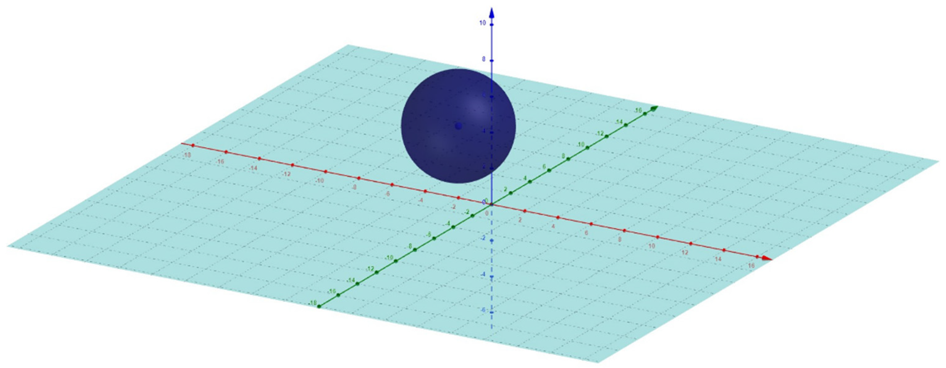
3.1. Sphere–Infinite Plane Interaction

Given a system that consists of a sphere $i$ with a center on point $C$, with radius $R$ and an infinite plane with its mass center on point $P$ (see Figure 2), the implicit function or general equation is defined [59] as follows:

$$a·\mathrm{x}+b·\mathrm{y}+c·\mathrm{z}+d=0$$

(9)

where $a$, $b$ and $c$ are the components of the vector normal to the plane in $x$, $y$ and $z$ axis, respectively. Considering the coordinates of the mass center, the value of $d$ is obtained as follows.

$$d=-a·r_x^P-b·r_y^P-c·r_z^P$$

(10)

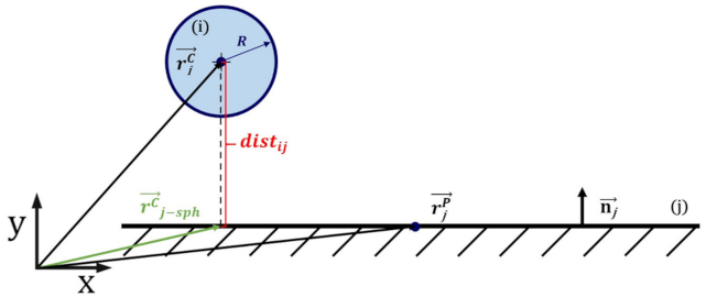
Once the general equation is completely defined, the distance from the center of the sphere to the plane, $dis{t}_{ij}$, is calculated (see Figure 3) as follows.

$$dis{t}_{ij}={\overrightarrow{\mathrm{n}}}_j·\overrightarrow{r_i^C}+d$$

(11)

The projection of the center of mass of the sphere on the plane is defined using the following value.

$${\overrightarrow{r^C}}_{j-sph}=\overrightarrow{r_i^C}-dis{t}_{ij}·{\overrightarrow{\mathrm{n}}}_j$$

(12)

This vector must be converted into local-frame plane coordinates, as it will be subsequently required to obtain the value of the relative contact velocity.

$${\overrightarrow{s^C}}_{j-sph}=A_j^{-1}·\left({\overrightarrow{r^C}}_{j-sph}-\overrightarrow{r_j^P}\right)$$

(13)

Then, the value of the indentation of the sphere into the plane, $\delta$, is calculated.

$$\delta =R-dis{t}_{ij}$$

(14)

Negative values of this term indicate that there is no contact between the sphere and the plane. The initial instance of contact takes place when $\delta$ = 0. Since this point, for each time step, the value of relative normal velocity between the bodies is calculated.

The parameters that must be specified to obtain the value of indentation in a sphere–infinite plane interaction according to the described algorithm are summarized in

Table 1. Summary of the parameters required to calculate the indentation between a sphere and an infinite plane.

Parameter	Description
$\overrightarrow{{\mathit{r}}_{\mathit{i}}^{\mathit{C}}}$	Position vector of the mass center of the sphere, i, in global-frame coordinates
$\overrightarrow{{\mathit{r}}_{\mathit{j}}^{\mathit{P}}}$	Position vector of the mass center of the plane, $j$, in global-frame coordinates
${\overrightarrow{\mathbf{n}}}_{\mathit{j}}$	Unit vector normal to the plane, directed towards the sphere, in global-frame coordinates
${\mathit{A}}_{\mathit{j}}$	Rotational transformation matrix of the plane
$\mathit{R}$	Sphere radius

.

This algorithm has provided reasonably good and consistent results when performing forward-dynamic analysis using the ODE integrators available in Matlab [60]. When dealing with multiple-impact scenarios (as will be subsequently described in Section 4), ODE113 has provided better outcomes at a minimal computing cost than the default ODE45 integrator.

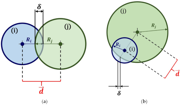
3.2. Sphere–Sphere Interaction

A system in which two spheres $i$ and $j$ with radii $R_i$ and $R_j$, respectively, come into contact is presented in Figure 4. In this case, two different interactions can take place according to the arrangement of the bodies: an external contact (Figure 4a) or an internal one (Figure 4b).

The algorithm for calculating the relative penetration between the bodies varies minimally between both cases. For an external contact, the expression that defines $\delta$ is as follows.

$$\delta =R_i+R_j-||\overrightarrow{d}||$$

(15)

The value of the indentation in an internal interaction is determined by the following equation.

$$\delta =R_i+R_j+||\overrightarrow{d}||$$

(16)

However, in this last case, the value of the largest radius is introduced with a negative sign. For both interactions, as long as $\delta$ is negative no contact will be happening; the start of the interaction occurs when $\delta$ = 0 (see Figure 5).

Likewise, the parameters that must be specified to obtain the value of relative penetration in a sphere–sphere interaction according to the described algorithm are summarized in

Table 2. Summary of the parameters required to calculate the indentation between two spheres.

Parameter	Description
$\overrightarrow{\mathit{d}}$	Vector between the mass centers of the two spheres
${\mathit{R}}_{\mathit{i}}$	Sphere $i$ radius
${\mathit{R}}_{\mathit{j}}$	Sphere $j$ radius

.

Once again, ODE45 and ODE113 have proved to deliver consistent results when carrying out dynamic analysis of systems with this kind of interactions and the latter is recommended for those cases when either there is a large difference between the values of the radii or the impact velocity is excessively large. In Section 4 further details and examples will be presented and developed.

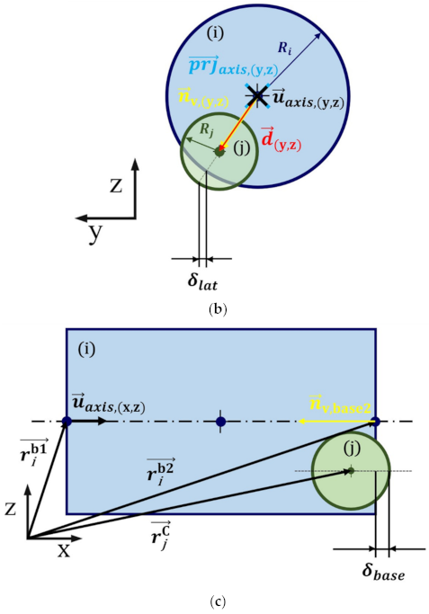
3.3. Sphere–Cylinder Internal Contact

In this case, the model consists of a cylinder $i$ and a sphere $j$ with radii $R_i$ and $R_j$, respectively. This interaction can be considered as a combination of the two previously described, as the bases of the cylinder can be characterized as sphere–plane interactions, while the contact between the lateral area of the cylinder and the sphere is defined by an algorithm inspired in the sphere–sphere case (see Figure 6).

For this latter contact, the projection of vector $\overrightarrow{d}$ on the cylinder axis, ${\overrightarrow{prj}}_{axis}$ must be obtained in the first place, given the unit vector of the axis, ${\overrightarrow{u}}_{axis}$.

$${\overrightarrow{prj}}_{axis}=\frac{\overrightarrow{d}·{\overrightarrow{u}}_{axis}}{||\overrightarrow{d}||}·{\overrightarrow{u}}_{axis}$$

(17)

The subtraction of vectors $\overrightarrow{d}$ and ${\overrightarrow{prj}}_{axis}$ provides vector ${\overrightarrow{n}}_{\mathrm{v}}$, which is normal to the cylinder axis and joins it to the center of the sphere (see Figure 7).

$${\overrightarrow{n}}_{\mathrm{v}}=\overrightarrow{d}-{\overrightarrow{prj}}_{axis}$$

(18)

Finally, the value of lateral indentation, ${\delta }_{lat}$, is obtained.

$${\delta }_{lat}=R_i+R_j+||\overrightarrow{d}||$$

(19)

Then, it will be verified if there is any contact taking place between the sphere and some of the bases of the cylinder. If contact is present, normal vectors will be directed towards the inside of the cylinder. The indentation on the base will be calculated using the algorithm developed in Section 3.1. In order to calculate the indentation on the base, the coordinates of the centers of both the sphere and the bases will have to be defined. All these variables are summarized in

Table 3. Parameters required to calculate the indentation between a cylinder and a sphere, according to the described algorithm.

Parameter	Description
$\overrightarrow{\mathit{d}}$	Vector between the mass centers of the cylinder and the sphere
${\overrightarrow{\mathit{u}}}_{\mathit{a}\mathit{x}\mathit{i}\mathit{s}}$	Unit vector in the direction of the cylinder axis
${\mathit{R}}_{\mathit{i}}$	Cylinder i radius
${\mathit{R}}_{\mathit{j}}$	Sphere j radius
$\overrightarrow{{\mathit{r}}_{\mathit{i}}^{\mathbf{b}\mathbf{1}}}$	Position vector of one of the bases of the cylinder, in global-frame coordinates
$\overrightarrow{{\mathit{r}}_{\mathit{i}}^{\mathbf{b}\mathbf{2}}}$	Position vector of the other base of the cylinder, in global-frame coordinates
$\overrightarrow{{\mathit{r}}_{\mathit{j}}^{\mathit{C}}}$	Position vector of the center of the sphere, in global-frame coordinates

.

This algorithm has also provided consistent outcomes when performing forward-dynamic analysis using the ODE integrators available in Matlab (see Section 4), being ODE113 better for those models in which there is a large difference between the values of the radii of the bodies.

3.4. Sphere–Rectangular Parallelepiped Interaction

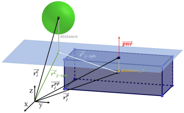
This interaction was developed as an evolution of the algorithm described in Section 3.1. Unlike the sphere–plane case, the planes here have finite extensions, so the complexity related to defining contact interactions increases considerably. The model in Figure 8 shows a sphere $i$ with radius $R$ and its center in $C$ and a rectangular parallelepiped $j$ with its mass center defined by point $P$.

Beginning from the sphere–plane case, a decision is made to analyze the contact detection for each face of the prism individually. In order to calculate the value of the indentation when the sphere hits one of edges, it will be necessary to decompose the contact direction into components normal to the faces that meet at that edge. In other words, the vector normal to the contact surface will always be a sum of the components in the normal directions to each one of the faces of the prism. However, to calculate all these terms it will be required to take into account the whole parallelepiped and all the possible contact cases that can happen between the sphere and the prism.

Apart from the aforementioned data, the inertia matrix of the regular parallelepiped must be provided:

$$J_{P,pln}=\frac{1}{12}·m_j·\left[\begin{array}{ccc}\left(w^2+h^2\right)& 0& 0\\ 0& \left(d^2+h^2\right)& 0\\ 0& 0& \left(w^2+d^2\right)\end{array}\right]$$

(20)

where $m_j$ denotes the prism mass and $d$, $w$ and $h$ denotes its dimensions in the $\xi \eta \zeta$ local-frame coordinates. This reference system has its origin in one of the corners of the parallelepiped (see Figure 9). The above tensor must be defined as a function of these dimensions and not numerically, as it will be subsequently used to calculate the coordinates of the edges of the prism and determine accurately if the sphere is in contact or not.

First, the values of $d$, $w$ and $h$ at each instant are calculated. They are denoted as $distanc{e}_x$, $distanc{e}_y$ and $distanc{e}_z$, respectively.

$$distanc{e}_x=d=\sqrt{\frac{12·\left(J_{P,pln\left(2,2\right)}-J_{P,pln\left(1,1\right)}+J_{P,pln\left(3,3\right)}\right)}{2·m_j}}$$

(21)

$$distanc{e}_y=w=\sqrt{\frac{12·\left(J_{P,pln\left(1,1\right)}-J_{P,pln\left(2,2\right)}+J_{P,pln\left(3,3\right)}\right)}{2·m_j}}$$

(22)

$$distanc{e}_z=h=\sqrt{\frac{12·\left(J_{P,pln\left(1,1\right)}+J_{P,pln\left(2,2\right)}-J_{P,pln\left(3,3\right)}\right)}{2·m_j}}$$

(23)

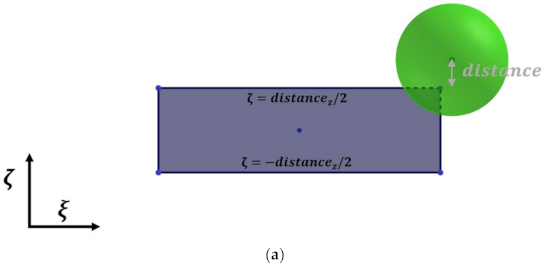
Descriptively, the algorithm developed here is defined with respect to the positive $\zeta$-axis plane (the upper face of the prism in Figure 9). Nevertheless, the concept is similar for the rest of faces of the parallelepiped. In the same manner as the sphere–plane interaction, the distance from the center of the sphere to the plane is calculated in the first place. In order to calculate this, a point of this plane and a vector normal to it must be defined (see Figure 10). The second value is known in terms of local-frame coordinates (in the case example, this will be (0, 0 ,1)), while in global-frame coordinates it will be given by the following expression:

$$\overrightarrow{pnv}=A_j·\left[\begin{array}{c}0\\ 0\\ 1\end{array}\right]$$

(24)

where $A_j$ is the rotation matrix that describes the orientation of the local system of the prism with respect to the global one, denoted as $xyz$. Regarding the point of the plane, $PP$, its coordinates are defined as follows.

$$\overrightarrow{r_j^{PP}}=\overrightarrow{r_j^P}+A_j·\left[\begin{array}{c}0\\ 0\\ distanc{e}_z/2 \end{array}\right]$$

(25)

Once the plane is completely defined, the distance from the center of the sphere to the plane (see Figure 11) is calculated using the general equation of a plane (see Equation (10)) and by obtaining the value of $d.$

$$distance=\overrightarrow{pnv}·\overrightarrow{r_j^{PP}}+d$$

(26)

At this point, the minimal distance between the sphere and the plane is a known quantity. If this value is greater than the radius of the sphere, there is no possibility that contact is happening. However, if this distance is less than the radius, it cannot be assured that no contact is taking place. Thus, it is necessary to calculate the projection of the center of the sphere on the plane coincident to the upper face of the prism, ${\overrightarrow{r^C}}_{j-sph}$ (see Figure 11).

$${\overrightarrow{r^C}}_{j-sph}=\overrightarrow{r_i^C}-distance·\overrightarrow{pnv}$$

(27)

This projection, in local-frame coordinates of the parallelepiped, being defined by the following expression.

$${\overrightarrow{s^C}}_{j-sph}=A_j^{-1}·\left({\overrightarrow{r^C}}_{j-sph}-\overrightarrow{r_j^P}\right)$$

(28)

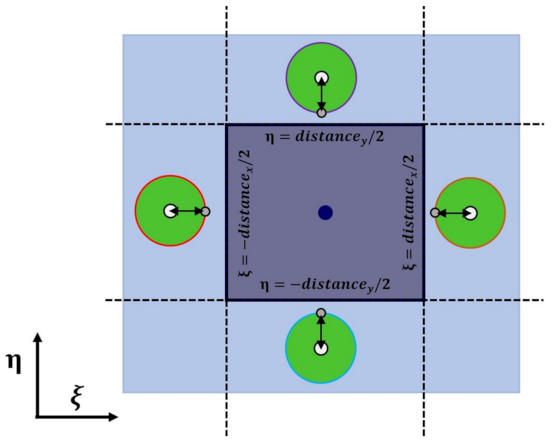
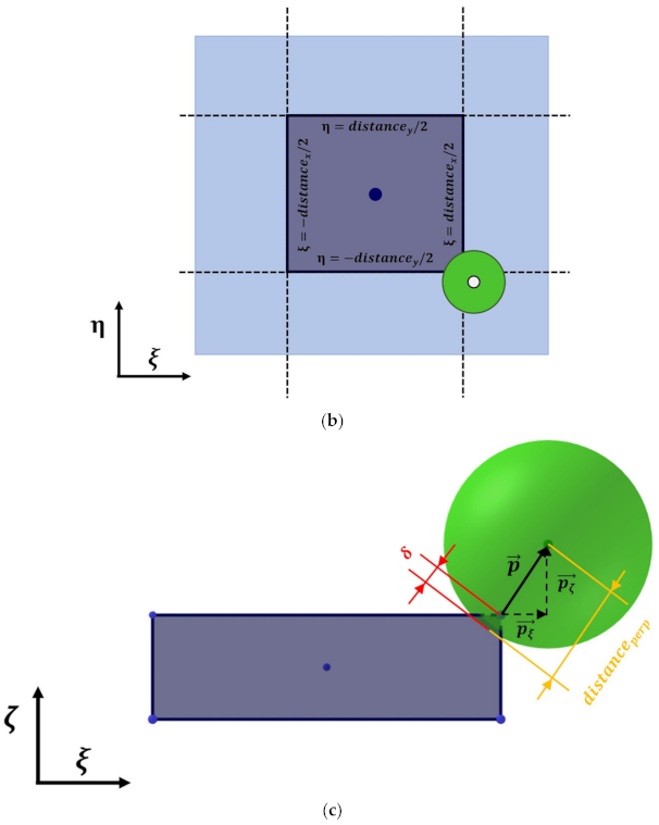
Then, it is verified if the projection of the sphere on the plane of the face of the prism intersects it. It will be compared, in local-frame coordinates of the prism, to each component of the projection of the center of the sphere on the plane, ${\overrightarrow{s^C}}_{j-sph, \xi }$ and ${\overrightarrow{s^C}}_{j-sph, \eta },$ with the values of the edges of the prism (see Figure 11.). The value of the sphere radius, $R$, will either be subtracted or added to this projection to consider any possible contact case that can happen with the corners of the prism. Thus, there will be no contact if any of the following conditions is met:

• ${\overrightarrow{s^C}}_{j-sph, \xi }-R>distanc{e}_x/2$: orange-edged sphere in Figure 12.
• ${\overrightarrow{s^C}}_{j-sph, \xi }+R<-distanc{e}_x/2$: red-edged sphere in Figure 12.
• ${\overrightarrow{s^C}}_{j-sph,\eta }-R>distanc{e}_y/2$: purple-edged sphere in Figure 12.
• ${\overrightarrow{s^C}}_{j-sph,\eta }+R<-distanc{e}_y/2$: blue-edged sphere in Figure 12.

Apart from these conditions, if the distance from the center of the sphere to the plane, in the normal direction relative to it, is greater than that of the sphere radius ($\left|distance\right|>\left|R\right|$), there will be no contact occurring either. If any of these conditions are met, there will be a contact interaction taking place between the sphere and the plane and the normal contact vector will have to be calculated. This vector, denoted by $\overrightarrow{p}$, joins the potential contact point of the parallelepiped with the center of the sphere, permitting the value of indentation to be obtained.

The system shown in Figure 13, in which the sphere is impacting with the parallelepiped, is proposed. The local-frame components of vector $\overrightarrow{p}$ will be calculated with the same method as how the different contact scenarios were verified previously:

• In local $\xi$ -axis, the value of the component of the normal contact vector will be the projection of the sphere on the plane, ${\overrightarrow{s^C}}_{j-sph, \xi }$, to which the value of half the dimension in this direction will be subtracted.

  $$\overrightarrow{p_{\xi }}={\overrightarrow{s^C}}_{j-sph, \xi }-\frac{distanc{e}_x}{2}·\left[\begin{array}{c}1\\ 0\\ 0\end{array}\right]$$

  (29)
• In local $\eta$ -axis, the value of the component of the normal contact vector will be ${\overrightarrow{s^C}}_{j-sph, \eta }$.

  $$\overrightarrow{p_{\eta }}={\overrightarrow{s^C}}_{j-sph, \eta }-\frac{distanc{e}_y}{2}·\left[\begin{array}{c}0\\ 1\\ 0\end{array}\right]$$

  (30)
• In the local $\zeta$ -axis the value of the component of the normal contact vector will be the distance from the center of the sphere to the plane.

  $$\overrightarrow{p_{\zeta }}=distance·\left[\begin{array}{c}0\\ 0\\ 1\end{array}\right]$$

  (31)

The module of vector $\overrightarrow{p}$ will provide the value of the distance between the bodies in the common normal direction of both bodies. This magnitude is denoted as $distanc{e}_{perp}$. Thus, the value of penetration will be given by the following expression

$$\delta =R-distanc{e}_{perp}$$

(32)

To reiterate, as long as $\delta$ maintains a negative value there will be no contact occuring. The interactions begins when $\delta$ becomes null. As in the previous sections,

Table 4. Parameters required to calculate the indentation between a sphere and a regular parallelepiped.

Parameter	Description
$\overrightarrow{{\mathit{r}}_{\mathit{i}}^{\mathit{C}}}$	Position vector of the mass center of the sphere i, in global-frame coordinates
$\overrightarrow{{\mathit{r}}_{\mathit{j}}^{\mathit{P}}}$	Position vector of the mass center of the parallelepiped j, in global-frame coordinates
$\mathit{R}$	Sphere i radius
${\mathit{m}}_{\mathit{j}}$	Mass of the parallelepiped
${\mathit{J}}_{\mathit{P},\mathit{p}\mathit{l}\mathit{n}}$	Inertia matrix of the parallelepiped, in local-frame coordinates
${\mathit{A}}_{\mathit{j}}$	Rotational transformation matrix of the prism

summarizes the parameters required to obtain the value of the relative penetration in a sphere–regular parallelepiped interaction according to the described algorithm.

The reader interested in other examples of contact detection algorithms for more complex solids is referred to the works by Choi [50] or Ambrósio [61]. In order to delve into the knowledge of contact force models, the authors recommend references [45,54].

In Section 4 the main issues arisen when modelling systems with this interaction are presented through a practical example.

4. Examples and Discussion

In this section, some practical examples based on the described algorithms are presented and developed, paying attention to the different issues experienced when dealing with contact scenarios and how these were overcome.

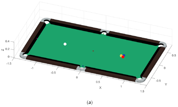
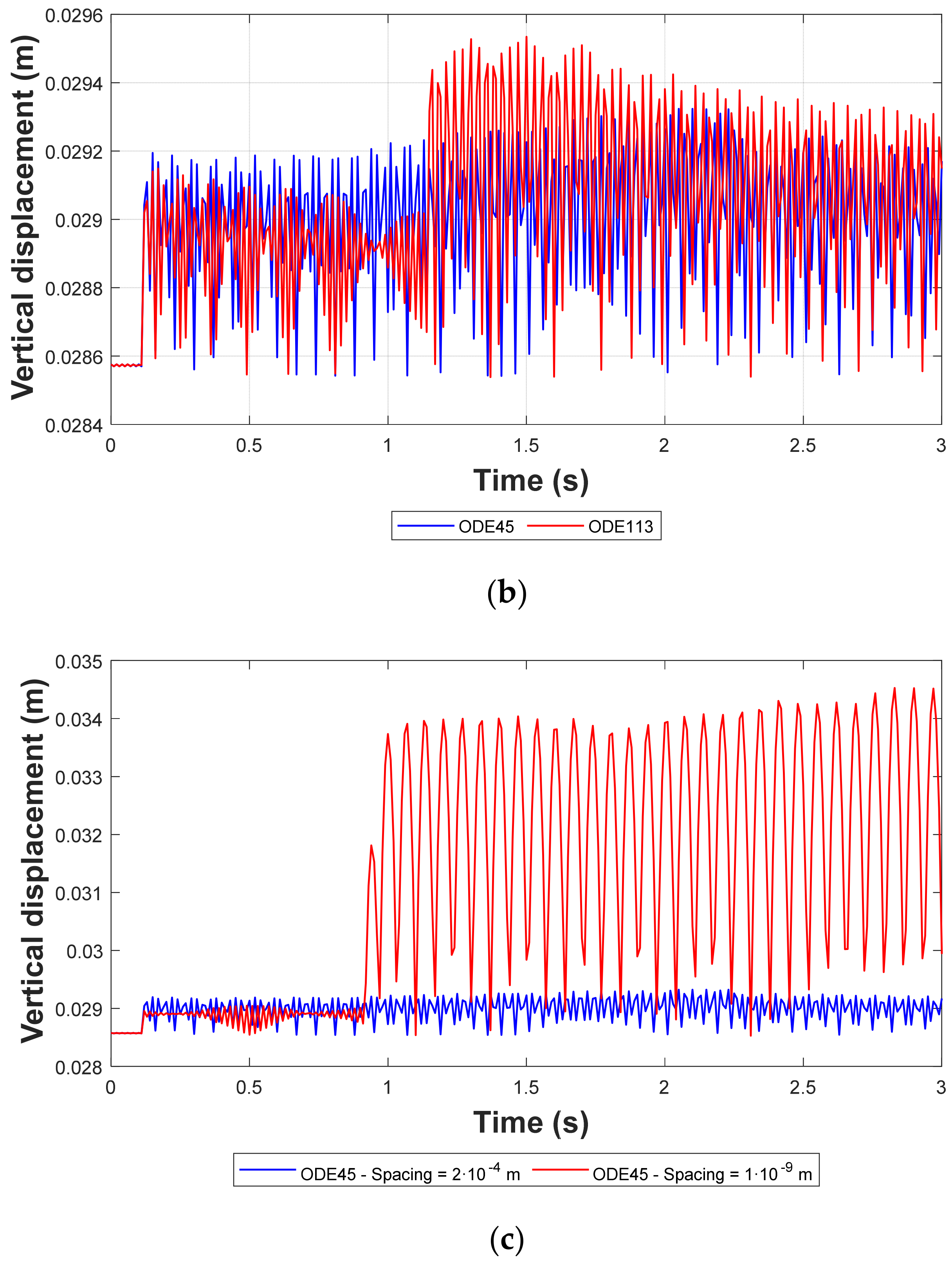
For the first two interactions, which are the sphere–infinite plane and the sphere–sphere cases, a simple model of a billiard that is presented and developed by the authors in [19] has been chosen (see Figure 14a). In this system, in which the balls can move freely in all directions, two different scenarios were considered: a permanent contact (between the balls and the cloth, as long as the ball is not hit and does not lift off the surface) and an intermittent one (between the balls and the cushions). When calculating the value of both friction and contact forces, the peculiarities of each interaction had to be taken into account. For this reason, a Hertzian contact force was chosen to calculate the value of normal force for the permanent contact, whereas the model proposed by Ambrósio proved to be the best choice to account for the friction force. For the contact interaction between the balls and the cushions, these being not-fully elastic, the model defined by Lankarani and Nikravesh was the optimal option to obtain the value of the normal, with Ambrosio’s model characterizing, once again, the friction phenomena. One of the problems associated with a fully elastic, permanent contact in the context of smooth modelling is the inclusion of vertical displacements of the balls due to the lack of energy dissipation, as can be observed in Figure 14b,c. As the balls were arranged closer between each other, this phenomenon increased, due to the fact that there was less time for energy dissipation associated with friction to happen before the ball–ball contact. This confirmed the fact that all contact events in the system were related to each other and had a decisive impact on the results. The solution that proved the best to reduce this effect was to introduce some degree of restitution in the permanent contact through a damping term.

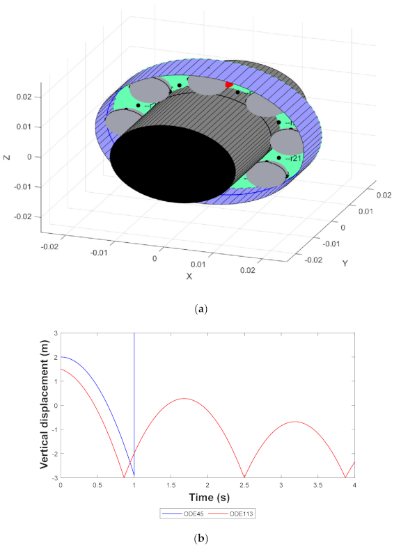
Focusing on the sphere–sphere interaction, a primitive model of a bearing with no axial loads is proposed (See Figure 15). In this case, there was a clear difference between the outcome provided by ODE45 and ODE113 when the clearance of the balls was large enough, i.e., the difference between the radii of the ball and the races. The reason for these results is the stiffness of the problem. The integrator is required to reduce the time step differential in order to detect the initial time of contact and it is required that the tolerances are reduced below the limit values. In addition to this, the computing time skyrocketed. In order to solve these problems, the ODE113 integrator was chosen and now obtains physically reasonable results for a not-fully elastic contact.

An evolved version of this bearing model was developed with the sphere–cylinder algorithm and, this time, permits the occurrence of axial loads. Keeping in mind the conclusions obtained from the previous tests, ODE113 was chosen by default as the integrator to solve the equations of motion. The results obtained are shown in Figure 16. This time, a shorter default time step was defined in order to obtain more accurate results.

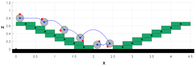
Lastly, for the sphere–parallelepiped contact interaction, the model shown in Figure 17. is proposed. In this case, the prisms are fixed bodies, while the ball can move freely. Some of the prisms include friction phenomena and others do not, but all of them are modelled as not-fully elastic impacts. As seen in Figure 17, the outcome is realistic from a physical point of view. However, if the opposite model is proposed, i.e., a fixed ball with a free prism, some tolerance problems arise even if ODE113 is used. A possible solution for this problem could be the definition of an algorithm of pre-contact detection such that the time step is adjusted when the initial instant of contact is going to happen. Given the stiffness of the problem, other ODE integrators could be also considered.

5. Concluding Remarks

The contact phenomena in the context of dynamics systems have been presented and studied. The two main existing approaches have been presented, along with their most distinctive features. Subsequently, a general algorithm for calculating the potential contact points of a system with two convex-shaped solids is developed. Then, contact interactions are introduced and described: sphere–infinite plane, sphere–sphere, sphere–cylinder and sphere–regular parallelepiped. Subsequently, some practical examples are presented and discussed and details are provided with respect to the issues arising during the design process. The ODE integrators that provide the most accurate results at a reasonable computing cost are defined and discussed. The default ODE45 integrator has proved to work reasonably well with most of the tested models. However, when extreme accuracy is required (for example, when defining the initial instant of contact) and the contact interaction is at some point, complex, some tolerance problems arise and it must be discarded in favour of stiffer algorithms.

Nevertheless, although this paper has focused on four simple interactions, the study of contact detection as well as the calculation of the magnitudes of the forces and the quantification of the phenomena associated to it is a research field under constant development, with almost continuous innovations.

References

- Rahnejat, H. Multi-body dynamics: Historical evolution and application. Proc. Inst. Mech. Eng. Part C J. Mech. Eng. 2000, 214, 149–173. [Google Scholar] [CrossRef] [Green Version]
- Shabana, A.A. Computational Dynamics; Wiley: New York, NY, USA, 1994; ISBN 978-0470686850. [Google Scholar]
- Nikravesh, P.E. Computer-Aided Analysis of Mechanical Systems; Prentice-Hall: Hoboken, NJ, USA, 1988. [Google Scholar]
- Haug, E.J. Computer Aided Kinematics and Dynamics of Mechanical Systems: Basic Methods; Allyn and Bacon: Boston, MA, USA, 1989. [Google Scholar]
- Shabana, A.A. Dynamics of Multibody Systems; Wiley: Hoboken, NJ, USA, 1989. [Google Scholar]
- Pfeiffer, F.; Glocker, C. Multibody Dynamics with Unilateral Contacts; Wiley: New York, NY, USA, 1996. [Google Scholar]
- Lankarani, H.M.; Nikravesh, P.E. Application of the canonical equations of motion in problems of constrained multibody systems with intermittent motion. In International Design Engineering Technical Conferences and Computers and Information in Engineering Conference; Design Engineering Division (Publication) DE; American Society of Mechanical Engineers: New York, NY, USA, 1988; Volume 14, pp. 417–423. [Google Scholar]
- Corral, E.; García, M.J.G.; Castejon, C.; Meneses, J.; Gismeros, R. Dynamic modeling of the dissipative contact and friction forces of a passive biped-walking robot. Appl. Sci. 2020, 10, 2342. [Google Scholar] [CrossRef] [Green Version]
- Marhefka, D.W.; Orin, D.E. A compliant contact model with nonlinear damping for simulation of robotic systems. IEEE Trans. Syst. Man Cybern. Part A Syst. Hum. 1999, 29, 566–572. [Google Scholar] [CrossRef]
- Marques, F.; Isaac, F.; Dourado, N.; Flores, P. An enhanced formulation to model spatial revolute joints with radial and axial clearances. Mech. Mach. Theory 2017, 116, 123–144. [Google Scholar] [CrossRef]
- Koshy, C.S.; Flores, P.; Lankarani, H.M. Study of the effect of contact force model on the dynamic response of mechanical systems with dry clearance joints: Computational and experimental approaches. Nonlinear Dyn. 2013, 73, 325–338. [Google Scholar] [CrossRef]
- Ambrósio, J. Train kinematics for the design of railway vehicle components. Mech. Mach. Theory 2010, 45, 1035–1049. [Google Scholar] [CrossRef]
- Shabana, A.A.; Zaazaa, K.E.; Escalona, J.L.; Sany, J.R. Development of elastic force model for wheel/rail contact problems. J. Sound Vib. 2004, 269, 295–325. [Google Scholar] [CrossRef]
- Ambrósio, J.; Dias, J. A road vehicle multibody model for crash simulation based on the plastic hinges approach to structural deformations. Int. J. Crashworthiness 2007, 12, 77–92. [Google Scholar] [CrossRef]
- al Nazer, R.; Rantalainen, T.; Heinonen, A.; Sievänen, H.; Mikkola, A. Flexible multibody simulation approach in the analysis of tibial strain during walking. J. Biomech. 2008, 41, 1036–1043. [Google Scholar] [CrossRef] [Green Version]
- Guess, T.M.; Thiagarajan, G.; Kia, M.; Mishra, M. A subject specific multibody model of the knee with menisci. Med. Eng. Phys. 2010, 32, 505–515. [Google Scholar] [CrossRef]
- Badie, F.; Katouzian, H.R.; Rostami, M. Dynamic analysis of varus knee using a subject-specific multibody model of the knee before and after osteotomy. Med. Eng. Phys. 2019, 66, 18–25. [Google Scholar] [CrossRef]
- Hirschkorn, M.; McPhee, J.; Birkett, S. Dynamic modeling and experimental testing of a piano action mechanism. J. Comput. Nonlinear Dyn. 2006, 1, 47–55. [Google Scholar] [CrossRef]
- Corral, E.; Gismeros, R.; Marques, F.; Flores, P.; García, M.J.G.; Castejon, C. Dynamic Modeling and Analysis of Pool Balls Interaction. In Computational Methods in Applied Sciences; Springer: Berlin/Heidelberg, Germany, 2020; Volume 53, pp. 79–86. [Google Scholar]
- Tasora, A.; Negrut, D.; Anitescu, M.; Mazhar, H.; Heyn, T.D. Simulation of massive multibody systems using GPU parallel computation. In Proceedings of the 18th International Conference on Computer Graphics, Visualization and Computer Vision, Plzen, Czech Republic, 1–4 February 2010. [Google Scholar]
- Flores, P. Concepts and Formulations for Spatial Multibody Dynamics; Springer International Publishing: Berlin/Heidelberg, Germany, 2015. [Google Scholar]
- Nikravesh, P.E. Planar Multibody Dynamics: Formulation, Programming and Applications; Taylor & Francis: Abingdon, UK, 2008. [Google Scholar]
- Pombo, J.C.; Ambrósio, J.A.C. Application of a wheel-rail contact model to railway dynamics in small radius curved tracks. Multibody Syst. Dyn. 2008, 19, 91–114. [Google Scholar] [CrossRef]
- Machado, M.; Flores, P.; Claro, J.C.P.; Ambrósio, J.; Silva, M.; Completo, A.; Lankarani, H.M. Development of a planar multibody model of the human knee joint. Nonlinear Dyn. 2010, 60, 459–478. [Google Scholar] [CrossRef]
- Chardonnet, J.R. Interactive dynamic simulator for multibody systems. Int. J. Hum. Robot. 2012, 9. [Google Scholar] [CrossRef] [Green Version]
- Peláez, G.; Rubio, H.; Souto, E.; García-Prada, J.C. Optimal Model Reference Command Shaping for vibration reduction of Multibody-Multimode flexible systems: Initial Study. In Advanced in Mechanisms and Machine Science; Springer: Cham, Switzerland, 2019. [Google Scholar]
- Wang, Z.J.; Cheng, L.D. Effect of material parameters on stress wave propagation during fast upsetting. Trans. Nonferrous Met. Soc. China (English Ed.) 2008, 18, 1189–1195. [Google Scholar] [CrossRef]
- Yamamoto, T.; Itoh, T.; Sakane, M.; Tsukada, Y. Creep-fatigue life of Sn-8Zn-3Bi solder under multiaxial loading. Int. J. Fatigue 2012, 43, 235–241. [Google Scholar] [CrossRef]
- Zeng, Y.; Song, D.; Zhang, W.; Zhou, B.; Xie, M.; Tang, X. A new physics-based data-driven guideline for wear modelling and prediction of train wheels. Wear 2020, 456–457, 203355. [Google Scholar] [CrossRef]
- Flores, P.; Lankarani, H.M. Contact Force Models for Multibody Dynamics; Springer International Publishing: Berlin/Heidelberg, Germany, 2016. [Google Scholar]
- Brogliato, B. Nonsmooth Mechanics: Models, Dynamics and Control, 3rd ed.; Springer International Publishing: Berlin/Heidelberg, Germany, 2016. [Google Scholar]
- Flores, P.; Machado, M.; Silva, M.T.; Martins, J.M. On the continuous contact force models for soft materials in multibody dynamics. Multibody Syst. Dyn. 2011, 25, 357–375. [Google Scholar] [CrossRef]
- Khulief, Y.A. Modeling of impact in multibody systems: An overview. J. Comput. Nonlinear Dyn. 2013, 8, 021012. [Google Scholar] [CrossRef]
- Alves, J.; Peixinho, N.; da Silva, M.T.; Flores, P.; Lankarani, H.M. A comparative study of the viscoelastic constitutive models for frictionless contact interfaces in solids. Mech. Mach. Theory 2015, 85, 172–188. [Google Scholar] [CrossRef]
- Lankarani, H.M. Contact/Impact Dynamics Applied to Crash Analysis. In Crashworthiness of Transportation Systems: Structural Impact and Occupant Protection; Springer: Dordrecht, The Netherlands, 1997; pp. 445–473. [Google Scholar]
- Lin, Y.C.; Haftka, R.T.; Queipo, N.V.; Fregly, B.J. Surrogate articular contact models for computationally efficient multibody dynamic simulations. Med. Eng. Phys. 2010, 32, 584–594. [Google Scholar] [CrossRef]
- Kim, S.W. Contact Dynamics and Force Control of Flexible Multi-Body Systems. Ph.D. Thesis, McGill University, Montreal, QC, Canada, 1999. [Google Scholar]
- Gilardi, G.; Sharf, I. Literature survey of contact dynamics modelling. Mech. Mach. Theory 2002, 37, 1213–1239. [Google Scholar] [CrossRef]
- Brach, R.M. Formulation of rigid body impact problems using generalized coefficients. Int. J. Eng. Sci. 1998, 36, 61–71. [Google Scholar] [CrossRef]
- Anitescu, M.; Potra, F.A.; Stewart, D.E. Time-stepping for three-dimensional rigid body dynamics. Comput. Methods Appl. Mech. Eng. 1999, 177, 183–197. [Google Scholar] [CrossRef]
- Wang, X.; Wang, Q. A LCP method for the dynamics of planar multibody systems with impact and friction. Lixue Xuebao Chin. J. Theor. Appl. Mech. 2015. [Google Scholar] [CrossRef]
- Pang, J.S.; Stewart, D.E. Differential variational inequalities. Math. Program. 2008, 113, 345–424. [Google Scholar] [CrossRef] [Green Version]
- Tasora, A.; Negrut, D.; Anitescu, M. Large-scale parallel multi-body dynamics with frictional contact on the graphical processing unit. Proc. Inst. Mech. Eng. Part K J. Multi-Body Dyn. 2008, 222, 315–326. [Google Scholar] [CrossRef]
- Mazhar, H.; Heyn, T.; Negrut, D.; Tasora, A. Using Nesterov’s method to accelerate multibody dynamics with friction and contact. ACM Trans. Graph. 2015, 34, 1–14. [Google Scholar] [CrossRef]
- Corral, E.; Moreno, R.G.; García, M.J.G.; Castejón, C. Nonlinear phenomena of contact in multibody systems dynamics: A review. Nonlinear Dyn. 2021, 104, 1269–1295. [Google Scholar] [CrossRef]
- Wang, Y.T.; Kumar, V. Simulation of mechanical systems with multiple frictional contacts. J. Mech. Des. Trans. ASME 1994, 116, 571–580. [Google Scholar] [CrossRef]
- Pratt, E.; Léger, A.; Jean, M. About a stability conjecture concerning unilateral contact with friction. Nonlinear Dyn. 2010, 59, 73–94. [Google Scholar] [CrossRef] [Green Version]
- Tasora, A.; Anitescu, M.; Negrini, S.; Negrut, D. A compliant visco-plastic particle contact model based on differential variational inequalities. Int. J. Non. Linear. Mech. 2013, 53, 2–12. [Google Scholar] [CrossRef]
- Xu, H.; Zhao, Y.; Barbic, J. Implicit multibody penalty-baseddistributed contact. IEEE Trans. Vis. Comput. Graph. 2014, 20, 1266–1279. [Google Scholar] [CrossRef] [PubMed]
- Choi, J.; Ryu, H.S.; Kim, C.W.; Choi, J.H. An efficient and robust contact algorithm for a compliant contact force model between bodies of complex geometry. Multibody Syst. Dyn. 2010, 23, 99–120. [Google Scholar] [CrossRef]
- Gonthier, Y.; McPhee, J.; Lange, C.; Piedbœuf, J.C. A regularized contact model with asymmetric damping and dwell-time dependent friction. Multibody Syst. Dyn. 2004, 11, 209–233. [Google Scholar] [CrossRef]
- Flores, P.; Ambrósio, J.; Claro, J.C.P.; Lankarani, H.M. Dynamic behaviour of planar rigid multi-body systems including revolute joints with clearance. Proc. Inst. Mech. Eng. Part K J. Multi-Body Dyn. 2007, 221, 161–174. [Google Scholar] [CrossRef] [Green Version]
- Zhang, Y.; Sharf, I. Validation of nonlinear viscoelastic contact force models for low speed impact. J. Appl. Mech. Trans. ASME 2009, 76, 051002. [Google Scholar] [CrossRef]
- Machado, M.; Moreira, P.; Flores, P.; Lankarani, H.M. Compliant contact force models in multibody dynamics: Evolution of the Hertz contact theory. Mech. Mach. Theory 2012, 53, 99–121. [Google Scholar] [CrossRef]
- Flores, P.; Ambrósio, J. On the contact detection for contact-impact analysis in multibody systems. Multibody Syst. Dyn. 2010, 24, 103–122. [Google Scholar] [CrossRef] [Green Version]
- Ebrahimi, S.; Hippmann, G.; Eberhard, P. Extension of the polygonal contact model for flexible multibody systems. Int. J. Appl. Math. Mech. 2005, 1, 33–50. [Google Scholar]
- Marques, F.; Flores, P.; Claro, J.C.P.; Lankarani, H.M. A survey and comparison of several friction force models for dynamic analysis of multibody mechanical systems. Nonlinear Dyn. 2016, 86, 1407–1443. [Google Scholar] [CrossRef]
- Machado, M.; Flores, P.; Ambrósio, J. A lookup-table-based approach for spatial analysis of contact problems. J. Comput. Nonlinear Dyn. 2014, 9, 041010. [Google Scholar] [CrossRef] [Green Version]
- Anton, H. Elementary Linear Algebra; Wiley: New York, NY, USA, 2013. [Google Scholar]
- Shampine, L.F.; Reichelt, M.W. The MATLAB ode suite. SIAM J. Sci. Comput. 1997, 18, 1–22. [Google Scholar] [CrossRef] [Green Version]
- Ambrósio, J. A general formulation for the contact between superellipsoid surfaces and nodal points. Multibody Syst. Dyn. 2020, 50, 415–434. [Google Scholar] [CrossRef]
Figure 1.
(a) General bodies with respect to the global reference system; (b) same bodies, with relative penetration. Both figures are presented in a 2D frame for ease of understanding.
Figure 2.
Simplified representation of a contact interaction between a sphere and an infinite plane.
Figure 3.
Calculation of the projection of the center of the sphere on the plane, .
Figure 4.
Simplified representation of the possible contact interactions between the two spheres: (a) external contact; (b) internal contact.
Figure 5.
Representation of the two possible interactions between two spheres: (a) external contact; (b) internal contact.
Figure 6.
Simplified representation of the internal contact between a cylinder and a sphere.
Figure 7.
Representation of the internal contact between the lateral surface of a cylinder and a sphere: (a) plane; (b) plane; (c) specific case in which there is contact with one of the bases.
Figure 8.
Simplified representation of the interaction between a sphere and a rectangular parallelepiped.
Figure 9.
Description of the dimensions of a rectangular parallelepiped and the location of its local reference frame.
Figure 10.
Location of point and vector .
Figure 11.
Projection of the center of the sphere on the plane coincident to the upper face of the parallelepiped.
Figure 12.
Different projections of the sphere on the plane coincident to the upper face of the parallelepiped.
Figure 13.
Case example in which there is contact happening between the sphere and the prism: (a) local -axis view; (b) local -axis view; (c) vector .
Figure 14.
Practical application example of the algorithms described in Section 3.1 and Section 3.2: (a) arrangement of the balls at t = 0 s; (b) evolution of z global coordinate of the cue ball as a function of the ODE integrators; (c) evolution of z global coordinate of the cue ball depending on the spacing between the balls of the rack.
Figure 15.
Practical application example of the algorithms described in Section 3.1 and Section 3.2: (a) arrangement of the bodies of the bearing; (b) evolution of vertical displacement of one of the balls, when clearance is large enough, without considering the inner race.
Figure 16.
Evolution of the position of the balls inside the cylinder for the proposed model.
Figure 17.
Evolution of the position of the ball rolling on a set of prisms arranged as stairs.