


Introduction
Globally, the glaciological community has only medium confidence in the prediction of ice discharge (Vaughan and others, Reference Vaughan2013), in part because of uncertainty in the viscous rheology of streaming ice that constitutes glaciers and is responsible for draining most of the ice sheets. Although we recognize how temperature, water content and microstructure affect ice flow (e.g. Barnes and others, Reference Barnes, Tabor and Walker1971; Duval, Reference Duval1977; Lile, Reference Lile1978; Weertman, Reference Weertman1983; Castelnau and others, Reference Castelnau, Thorsteinsson, Kipfstuhl, Duval and Canova1996, Reference Castelnau1998; Goldsby and Kohlstedt, Reference Goldsby and Kohlstedt2001; Cuffey and Paterson, Reference Cuffey and Paterson2010; Minchew and others, Reference Minchew, Meyer, Robel, Gudmundsson and Simons2018; Haseloff and others, Reference Haseloff, Hewitt and Katz2019), we do not have a robust understanding of how these factors are distributed in natural settings, particularly in locations of high mechanical significance.
These critical locations include the lateral and basal margins of ice streams and glaciers, which deform under different conditions than do the fairly well studied ice beneath divides. As such, knowledge of, for example, fabric, grain size, temperature and interstitial water content at ice divides is not directly transferable to the margins of streaming ice. However, measuring rheologically relevant parameters in the margin of streaming ice presents a logistical challenge due to high deformation rates, safety considerations and internal structures that complicate geophysical surveys. Nevertheless, knowledge of the magnitude and distribution of those parameters are critical given that margins, whether frozen or sliding, commonly provide the majority of the resistance to flow (cf. Raymond and others, Reference Raymond2001).
Measuring fabric is a particularly important challenge to overcome. As the early experiments determined (McConnel and Kidd, Reference McConnel and Kidd1888), ice exhibits strong mechanical anisotropy in the viscous regime. Additional experiments and increasingly sophisticated numerical models illustrate that fabric and other microstructural variables can have a large effect on ice kinematics (e.g. Barnes and others, Reference Barnes, Tabor and Walker1971; Ashby and Duval, Reference Ashby and Duval1985; Alley, Reference Alley1992; Castelnau and others, Reference Castelnau1998; Goldsby and Kohlstedt, Reference Goldsby and Kohlstedt2001; Thorsteinsson and others, Reference Thorsteinsson, Waddington and Fletcher2003; Pettit and others, Reference Pettit, Thorsteinsson, Jacobson and Waddington2007; Martín and others, Reference Martín, Gudmundsson, Pritchard and Gagliardini2009, Reference Martín, Gudmundsson and King2014; Ma and others, Reference Ma2010; Treverrow and others, Reference Treverrow, Budd, Jacka and Warner2012; Budd and others, Reference Budd, Warner, Jacka, Li and Treverrow2013; Minchew and others, Reference Minchew, Meyer, Robel, Gudmundsson and Simons2018; Hruby and others, Reference Hruby2020). Nevertheless, a few studies report marginal microstructures, particularly fabric from direct observation (Hudleston, Reference Hudleston, Saxena and Bhattacharji1977, Reference Hudleston1980; Jackson, Reference Jackson1999; Hellmann and others, Reference Hellmann2021; Monz and others, Reference Monz2021) (Jackson and Kamb, Reference Jackson and Kamb1997). Although some have calculated the effect of fabric on rheology based on observational data (Minchew and others, Reference Minchew, Meyer, Robel, Gudmundsson and Simons2018), without more in situ measurements, questions remain about how well models and experiments reflect natural settings.
Below, we describe the fabric and related microstructure from two surface-to-bed cores and one partial core in the lateral margin of a small polythermal glacier in Alaska. We find systematic changes in grain size and shape, as well as bubble aspect ratio, consistent with a strain gradient. To our knowledge, our study is the first to report fabric from surface to bed within the margin of a temperate glacier, and only the third from any lateral margin (cf. Jackson, Reference Jackson1999; Monz and others, Reference Monz2021). The fabric is relatively weak, but the fact that any fabric develops in the short flow distance of relatively slow-moving ice in a water-rich environment indicates that substantial fabric development is probable in larger glaciers and ice streams. As such, fabric is likely to play a large mechanical role in controlling the kinematics of those settings.
Field setting
Jarvis Glacier, a north-flowing glacier in the eastern Alaska Range (−145.68° W, 63.48° N), is ~5.2 km2 in surface area, ~8 km long and up to ~220 m thick, with at least one cirque-based tributary, and a headwall elevation of ~2000 m (Fig. 1). The glacier undergoes a nearly right angle turn a quarter of the way down its length, and has an overall surface slope of ~5°. The bedrock valley is approximately U-shaped, with typical 10–100 m wavelength, 1–10 m amplitude irregularities. The tributary (Fig. 1b) lies 1 km upstream of our study site and, based on debris lines (Fig. 1c), contributed the ice examined in this study, part of the western quarter of the glacier.
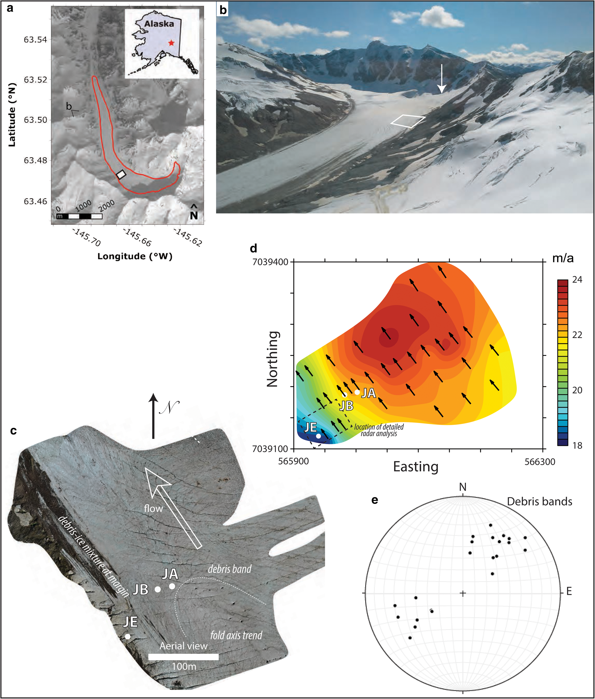
Fig. 1. Geographic and glaciological frameworks of the study area. (a) Location of Jarvis within the eastern Alaska Range, with the study area marked by the white rectangle. View direction for (b) is marked. Basemap image provided by the Polar Geospatial Center. (b) Oblique view of the field site (view to the southeast), with the core ice origin (arrow) labeled. Rectangle indicates the study area. (c) Aerial view of core site with no snow cover and core locations marked. (d) Stake-derived velocity map of field site. (e) Lower hemisphere stereographic plot of orientations of debris bands measured at the surface.
Velocity stake data (Fig. 1d) indicate that the glacier flows up to 24 m a−1 in the vicinity of the study site, decreasing to 18 m a−1 near the margins. These measurements indicate a transverse surface shear strain rate of 1.5×10⁻⁹ s−1 between JA and JE, with no evident longitudinal velocity gradient at the study area. This velocity pattern suggests most of the residual velocity is accommodated by slip at the margin. The lateral glacier boundary itself is difficult to define due to debris coverage. Orientations of debris bands measured at the surface are somewhat variable, with most having a moderate northwest or southeast dip (Fig. 1e), consistent with fold axes observed in the field. Qualitative observations reveal more intense crevassing near JE than near JA. Mean englacial temperatures are warmer than −2°C (Lee, Reference Lee2019). Jarvis Glacier is losing mass, with the 2016 season seeing 2 m of surface ice loss near the study site. Approximate average temperatures at a nearby meteorological station ridge, 630 m WNW and 25 m higher than the drill site, are 5°C in the summer and −13°C in winter (http://ine.uaf.edu/werc/projects/jarvis/offglacier.aspx).
Methods
Radar
We used a Geophysical Survey Systems Incorporated (GSSI) SIR-4000 ground-penetrating radar (GPR) control unit coupled with a GSSI 100 MHz antenna to select appropriate ice core sites and place micro-structural observations from ice cores into a broader context. Radar profiles were recorded with a Trimble 5700 survey unit and Zephyr GPS antenna operating at 1 Hz to georeference data. Additionally, we collected profiles spaced 10 m apart within a 100 m by 60 m grid near the valley wall and collected a longer profile perpendicular to the valley wall. Data were collected in time mode at 1024–2048 samples per scan and 24–40 scans per s. Profiles were time-zero corrected, distance-normalized and stacked three times to improve signal to noise ratios. We also applied background, low (300 MHz), and high pass (25 MHz) filters to reduce noise.
Cores
Using the radar data, we selected core sites in order to minimize the probability of encountering debris bands. We retrieved the cores using a 3-in Badger Eclipse rotary drill during April and May 2017. The cores reported here are JA (63.4750° N, 145.6753° W, 1621 m), JB (63.4749° N, 145.6759° W, 1625 m) and JE (63.4743° N, 145.6766° W, 1625 m), collected ~100, ~75 and ~25 m from the lateral boundary (Fig. 1). Three additional cores were attempted, with englacial debris preventing access to the bed. Core segments were logged, moved to a −20°C freezer on site, then flown to −20°C cold rooms at the Fairbanks, AK, Cold Regions Research and Engineering Laboratory. There, we photographed all core segments on a light table and selected a subset of core segments to return to Maine. During shipping, cores remained below −15°C. Storage at a commercial freezer facility in Maine is maintained at −20°C or colder. We were unable to retain azimuthal data for the core segments.
Televiewer
Using a QL40 OBI optical televiewer from Advanced Logic Technology, we recorded the intensity of light return of the borehole walls with depth. The televiewer produces an unwrapped image of the wall, converting a cylinder in real space to a 2-D image. Thus, a planar dipping layer appears as a sinusoid, with the peak and trough representing the azimuth of the up- and down-dip directions. Using this relationship, we calculated the orientation of dipping layers throughout the borehole and characterized them as light, dark or intermediate. In addition, by comparing photographs of the core with the televiewer images, we attempted to document the azimuth of each core segment. We concluded that the uncertainty was too high to have confidence in the determinations; therefore, although we report azimuthal data for the borehole wall imagery, we present all core data with no azimuthal component.
Microanalysis
For selected core segments, we prepared thin sections for imagery and slabs for electron backscatter diffraction (EBSD) analysis. All sections are in plan view, perpendicular to the core axis, with a downhole viewing direction. We photographed whole thin sections on a light table at multiple orientations relative to crossed polarizing filters. For samples cut from a single block, we manually traced complete grain boundaries (i.e. no edge grains) and bubbles. Using ImageJ (https://imagej.nih.gov/ij/), we calculated grain and bubble geometric statistics. Here we report grain size, grain circularity and bubble aspect ratio. We report grain size as the diameter of a circle with an area equivalent to that measured in the grain.
EBSD analysis employed a Tescan Vega II electron microscope fitted with a tungsten filament and a custom-built liquid nitrogen cooled stage. Hardware and software were a EDAX Digiview IV camera and OIM Data Collection v. 5.3. To prepare the sample, we manually cut, shaved and mechanically abraded (using sandpaper and polishing cloths) the ice block in a −20°C freezer to ~5 cm×7 cm×1 cm, generating a smooth, flat surface. Although we cut most sections from a single layer of ice, for segments with very large grains (multi-cm), we cut strips from two or three segments spaced farther apart than the grain size in order to incorporate a greater number of grains in a single analysis (cf. Monz and others, Reference Monz2021). We froze the sample to a similarly sized copper plate. We prepared all samples in a cold room then transferred them to the electron microscope laboratory in a cooler containing liquid nitrogen, thus preventing frosting. We introduced samples to the electron microscope through a nitrogen-gas flooded glovebox onto a copper plate precooled to ~ −150°. In most cases, frosting was sufficiently minimal that we were able to begin analysis as soon as the system achieved our target pressure of 5 Pa. For some samples, we cycled the pressure (see Prior and others, Reference Prior2015) to reduce frost. During analyses, sample temperatures were typically −110 to −100°C.
Although total area and step size varied from sample to sample, typical step sizes were 60 μm, collected at a tilt angle of 60° and working distance of ~35 mm with a dwell time of 50 μs. Beam conditions were ~125 nA with 15 kV accelerating voltage. We utilized 60°, rather than the more common 70°, tilt for the samples in order to image as large as possible within the geometrical constraints of the electron microscope chamber. Tests indicated that the different tilt did not affect data quality or accuracy.
EBSD data processing
Although the EDAX indexing rate was high (typically better than 90%), accuracy due to symmetry challenges was not sufficiently high to permit automatic grain analyses. However, we were able to manually identify grains. By validating orientations through multiple point analyses in each grain, we produced a dataset with one point per grain for each sample. Some orientations (<5% of the dataset) were particularly challenging for the software to index accurately, even though the diffraction pattern was sufficiently strong to identify bands. In nearly all of those cases, we manually indexed the diffraction pattern. In the end, our dataset represents over 99% of the grains in the slabs. Because of the orientation artifacts within grains, we did not calculate grain geometry statistics from EBSD data, but rather utilized the data from the thin sections made from ice adjacent to the EBSD slab.

Fig. 2. Profiles of 100 MHz ground-penetrating radar grid survey along the lateral margin of Jarvis Glacier showing bedrock (black arrows), ice with low- and high-signal scattering (separated by dotted white line), inferred debris bands which act as water conduits advected into the ice from the bed due to ice flow (white arrows), and successful drill site JE. Location of the radar grid shown in Figure 1. Depth is derived from two way travel time (TWTT) based on a relative permittivity of ice of 0.169 m ns−1.
From each sample's grain orientation dataset, we calculated an orientation tensor for c-axes, a mathematical construct describing the weighted distribution of c-axes in three dimensions (cf. Allmendinger and others, Reference Allmendinger, Cardozo and Fisher2011).
The components of a symmetric 3-by-3 orientation tensor a are:

where n is the number of points and x, y and z are the spatial components of the unit vector describing the c-axis orientation for the ith grain.
Although the tensor has both shape and orientation, because of the lack of azimuth control on our samples, we compared only the length and inclination of the principal axes (i.e. eigenvalues and eigenvectors) of the tensor between samples.
Macroscopic observations
We employed radar surveys to determine ice thickness, select areas for coring with minimal englacial debris and determine the thermal structure of Jarvis Glacier as it relates to each core site. Surface-to-bedrock 100 MHz GPR profiles collected within the local study area revealed ice thicknesses reaching over 100 m and 10–22 m of a low-scattering layer overlying higher scattering (Fig. 2). Past studies have interpreted this as a polythermal architecture, with cold ice over warm, but the scattering increase could be due solely to ice with low water content overlying ice with high water content (e.g. Campbell and others, Reference Campbell2012). Temperature data (Lee, Reference Lee2019) suggest that all ice is warmer than −2°C.

Fig. 3. Macroscale core and borehole data. (a) Depths of samples used for this study. (b) Example optical televiewer image of borehole wall. With the ‘unwrapped’ borehole wall image, planes appear as sinusoids (e.g. annotated with red dotted line). (c) Example televiewer image of ice core illustrating bands, which are variably present throughout the cores. (d) Lower hemisphere stereographic plot of orientations of bands determined from televiewer images.
Based on abundant water, resistance to drilling deeper and GPR surveys, we infer that JA and JE reached the bed at 80 and 18 m, respectively, whereas JB terminated at a debris band at 30 m. The coring and GPR results suggest a bedrock slope reaching 41°. The local 100 by 60 m GPR data grid collected near the valley wall revealed debris or shear bands dipping up-glacier at 10–15°. Using an interpretation scheme focused on the phase polarity of the radar triplet (Arcone and others, Reference Arcone, Lawson and Delaney1995), these horizons, in most cases, suggested a transition to very high permittivity values relative to the ice above. We attribute that transition to high water content, which is consistent with observations of water flowing out of borehole walls at certain depths while drilling.
Visual core logging at the time of extraction and in a cold room with transmitted light revealed that the cores were heterogeneous in many aspects, including bubble size, bubble density, presence of debris layers, presence of bubble-free layers and fractures (Fig. 3). Many distinct structural features have length scales of centimeters (Fig. 3c). Below 6 m in JA, 21 m in JB, and throughout JE, the extracted chips and/or cores were commonly wet; some core segments were wet enough to characterize as slushy. Abundant water resided at the bottom of borehole JA. Bands measured at the surface had a general dip distribution to the northeast and southwest at a moderate angle. Layers measured in the borehole walls using optical televiewer images show a more diffuse northeast-southwest pattern, with no strong concentrations. JA and JE exhibit overlapping band orientation distributions, with some unique areas (Fig. 3d): JE contains nearly exclusively southwest-dipping bands, whereas JA is more dispersed northeast to southwest. Consistent with surface band measurements (Fig. 1e), the strike of almost all bands recorded in the borehole walls is subparallel to the flow direction. We discerned no substantive difference in orientation of the dark versus light bands. Tiltmeters installed in JA and JE indicate shear along horizontal planes (i.e. change in longitudinal velocity with depth) in both holes, with a higher degree in JE (Lee, Reference Lee2019). The horizontal-plane shear strain rate reported by Lee and others (Reference Lee2020) at the bottom of JE is comparable to the vertical-plane shear strain rate indicated by the velocity stake data. The base of JA appears to deform at approximately half that rate. Moreover, flow at JE appears to be more sensitive to stress via a higher stress exponent (Lee and others, Reference Lee2020).

Fig. 4. Representative images of thin sections, illustrating grain shape and size distribution. Fine-grained areas on the perimeter are where water seeped under the sample.
Microstructural observations
We performed EBSD analysis on 19 samples for JA and eight samples from JE and light microscopy for 13, 8 and 6 samples from, respectively, JA, JB and JE. Although we analyzed each core with depth, differences therein were smaller than between cores; as such we focus most of our discussion on the latter. See Tables S1 and S2 for additional information and Figures 4 and S1 for thin section images.
General description. As with the macroscopic observations, many microstructures are heterogeneous on the centimeter scale, but heterogeneity is not ubiquitous. To pick two metrics, grain size and bubble distribution, in JA, nine out of 20 samples shown in Figure S1 exhibit bimodal grain size distributions and eight out of 13 samples in which we mapped bubbles exhibit a patchy distribution. For JB, the frequency is three out of eight for grain size and two out of eight for bubble distribution. For JE, the frequency is one out of six for grain size and three out of eight for bubble distribution. Grains in JE, including fine grains, are more lobate than those in JA or JB. In most samples, grain lobes exhibit one or more straight segments. Triple junction angles in all sample span a wide range; no samples manifest a strong foam texture appearance.

Fig. 5. Bubble aspect ratio measurements. (a) Number frequency histograms of bubble aspect ratios for all samples (thin lines) and core averages (thick lines). (b) Cumulative frequency plots, using the same dataset and legend as in (a). (c) Plot of average bubble aspect ratio, with standard deviation, versus depth.
Bubble aspect ratio. The bubble aspect ratio distribution (Fig. 5) is relatively consistent within each core, as well as across JA and JB. Both of these cores exhibited right-skewed distributions, with, respectively, 25 and 28% of the bubbles in the range of 1.05–1.15 (Fig. 5). Aspect ratios >2 constitute 9 and 1.6% of the total. Aspect ratios in core JE data are left-skewed and distinct from JA and JB. Approximately 24% of all bubbles have aspect ratios >2.

Fig. 6. Grain size measurements. (a) Number frequency histograms of grain sizes for all samples (thin lines) and core averages (thick lines). (b) Cumulative frequency plots, using the same dataset and legend as in (a). (c) Plot of average grain size, with standard deviation, versus depth.
Grain size. Although grain size can be heterogeneous at the thin section scale, the overall distribution throughout each core is relatively constant (Fig. 6). JA has dominant small grain populations, under 2 mm diameter. JB has a mixture of dominant areas of small and large populations. JE largely comprises large grains, with many over 5 mm diameter, although one sample has extensive small grains.

Fig. 7. Grain shape measurements. (a) Number frequency histograms of circularity for all samples (thin lines) and core averages (thick lines). (b) Cumulative frequency plots, using the same dataset and legend as in (a). (c) Plot of average circularity, with standard deviation, versus depth.
Grain circularity. Circularity measures the full perimeter of an object relative to that of its contained area:

where A is the area of the grain and P is the perimeter. Hexagonal grains have a circularity of 0.907. Core JA exhibits some coherence down core, with most grains exhibiting circularity from 0.6 to 0.8 (Fig. 7). JB and JE exhibit little coherence, in part due to the small number of grains in some samples, and therefore contain a wide range of grain shapes, with most circularities from 0.35 to 0.8. However, averages across the data profiles – thick lines in Figure 7 – reveal that JE is skewed toward lower values than are JA and JB.

Fig. 8. Representative minimally processed inverse pole figure maps (JA91, JE24), illustrating indexing rate (unindexed pixels are black) and that grains are discernible for manual identification. Angular drift within each scan is due to the long working distance.
Crystallographic orientation. The data reported here are one point per grain, with no additional processing (Fig. 8). We recognize the possibility (Fan and others, Reference Fan, Hager, Prior, Cross, Goldsby, Qi, Negrini and Wheeler2020) (Monz and others, Reference Monz2021) that highly lobate grains may be represented in the dataset more than once, and discuss this further below. With that acknowledgement, consistent with the grain size data (Fig. 6), we observed a wide range of number of grains per sample, from n = 13 to 454.
Pole figures (Figs 9, 10) illustrate that some non-isotropic fabric exists, visible in both the c- and a-axes. The orientation tensors of c-axes for each sample (Fig. 11; Table S1) reveal significant overlap between JA and JE, but also some distinctions. A ‘Flinn’ style diagram (Fig. 11a), in effect describing the shape of the aggregate crystallographic fabric, reveals that the orientation tensor for JE is more prolate than that of JA, as well as consistently farther from isotropy. The ratio of the maximum to minimum principal axes of the orientation tensor (Fig. 11b) indicates that JE has a stronger fabric than JA at comparable depth. JA increases in fabric intensity with depth, approaching that of JE at their respective bases. The base of JA contains large grains, so the grain statistics at that depth yield higher uncertainty.

Fig. 9. Upper hemisphere stereographic plots of c-axis orientations for samples from JA and JE. View is down, normal to the ice core axis. Numbers to the upper left of each diagram indicate the sample number; numbers to the upper right are the sample depth in meters; numbers to the lower left are the number of grains. Principal components of the orientation tensor (gray squares) are scaled to axis magnitude. For JA10, we present large and small grains separately.

Fig. 10. Upper hemisphere stereographic plots of a-axis orientations for samples from JA and JE. View is down, normal to the ice core axis. Numbers to the upper left of each diagram indicate the sample number; numbers to the upper right are the sample depth in meters; numbers to the lower left are the number of grains. For JA10, we present large and small grains separately.

Fig. 11. (a) Flinn-type diagram illustrating the shape of the orientation tensor. A girdle plots along the x-axis whereas a single pole plots along the y-axis. Isotropically distributed c-axes plot near the origin. JA points plot closer to the origin than JE points. JE also tends more toward single pole than girdle. However, in no case is the fabric strong. With depth, JA fabrics lie farther from the origin. Point size scaled by number of measurements in the sample. (b) Ratio of the maximum to minimum values of the principal axes of the orientation tensor, which represents the magnitude of the variance from isotropy. The values of JA are less than those of JE for the same absolute depth, but approach the same at the bottom of the core. Point size scaled by number of measurements in the sample. (c) Angle of inclination for c-axes in JA and JE. JA has a more evenly dispersed distribution, approximately the theoretical random distribution, whereas JE has more c-axes close to horizontal.
The a-axes of all samples range in distribution consistent with the c-axis patterns (Fig. 10). Several samples display relatively dispersed a-axes (e.g. JA22, 106), but many contain a diffuse girdle (e.g. JA74, JA91, JE12). The JE samples have stronger girdle patterns than do the JA samples, consistent with the more prolate c-axis orientation tensors (Fig. 11a, Table S1). No sample displays strong clusters of a-axes.
Discussion
Optical observations
Grain size is similar within each of the cores, but the patterns differ between cores (Fig. 6). On average, grains closer to the margin are coarser. Grain shape, as determined by circularity, is also somewhat different. Only core JA has a coherent grain shape pattern, with most samples displaying a similar distribution of circularity (Fig. 7), peaking at 0.7 and having a long tail toward 0.3. JB and JE have some samples that display a similar circularity profile as JA, but also several samples that exhibit highly variable patterns. As noted previously, the low number of grains in some samples may introduce some of the noise in the data. The somewhat faceted geometry of the lobate grain boundaries may be due to the high homologous temperature (cf. Piazolo and others, Reference Piazolo, Bestmann, Prior and Spiers2006) or the presence of liquid water during recrystallization or post-extraction liquid water crystallization.
To a first order, bubble aspect ratios relate to the degree of finite strain. JE exhibits higher aspect ratios than JA or JB, consistent with the strain measurements derived from the tiltmeter data (Lee and others, 2019), the velocity stake measurements, and standard model predictions.
In sum, the optically visual microstructure indicates that core JE experienced more strain than JA and JB, and that a larger grain size and less circular grain shapes correlate with the strain difference. The grain sizes lie in a range where they are unlikely to have a significant effect on the local ice rheology, although strain may have localized along fine-grained bands.
Crystallographic orientation fabric distribution
In this section, we compare the distribution of crystallographic axes between the cores in more detail. Our main focus is to define the rheologically significant patterns to the extent possible and identify any differences between the margin of streaming ice (JE) and ice closer to the centerline (JA). JA is not at the center of the ice, but aerial imagery suggests that it occupies a strain regime similar to the centerline (Fig. 1). Although no strong fabrics (e.g. single pole, multipole, girdle) developed in any sample, we do observe some notable relationships.
First, c-axes in JE are more clustered near horizontal than are those in JA (Figs 9, 11c). We interpret this to mean that, for the most part and consistent with theory, the highly inclined c-axes have rotated toward the horizontal and/or preferentially grown in this orientation with increased strain in JE. The c-axis orientations at the base of JA are of intermediate inclination values compared to JA and JE. With no azimuth control, we cannot evaluate the horizontal orientation of any samples relative to the shear plane.
Second, even without azimuth control, we can evaluate the shape of the orientation tensor and find that JE has on average more concentrated c-axes than does JA (Fig. 11a). Moreover, the shape of the c-axis distribution is closer to prolate (single pole) than oblate (girdle). However, the shape of the orientation tensors for JA and JE do exhibit some overlap.
Third, although slight, we observe a change in crystallographic fabric intensity in JA with depth. This is best seen in the increase in the ratio of the maximum and minimum principal axes of the orientation tensor (Fig. 11b). Again, this is consistent with theory in that ice near the bed should have higher shear strain and therefore develop stronger fabric. Taken at face value and assuming that the area sampled represents the local volume, the strength of the fabric at the base of JA approaches the strength of the fabric throughout JE.
The a-axis patterns are consistent with the c-axis patterns and suggest that there is little clustering of a-axes, promoting the notion that the ice sample rheology approaches transverse isotropy. The lack of a-axis clustering contrasts somewhat with observations of natural and experimental sample sets that display a mixture of clusters and girdle distributions (Miyamoto and others, Reference Miyamoto2005; Wongpan and others, Reference Wongpan, Prior, Langhorne, Lilly and Smith2018; Journaux and others, Reference Journaux2019; Qi and others, Reference Qi2019; Monz and others, Reference Monz2021). In both of our cores, the microstructure, including fabric, is heterogeneous with depth, indicating that the mechanical history and structure are not completely systematic.
Implications for fabric formation in other settings
By almost any measure, our measured fabrics are relatively weak. However, as with other microstructural metrics (Figs 6, 7), JE has developed a fabric distinct from that of JA (Figs 9, 11). This fabric gradient is consistent with the strain gradient, as suggested by surface features (Fig. 1c), tiltmeter data (Lee and others, Reference Lee2020) and bubble morphology (Fig. 5). In general, fabric formation is likely to be strongest where dislocation creep is the dominant deformation mechanism and as flow distance increases (Russell-Head, Reference Russell-Head1985; Castelnau and others, Reference Castelnau, Thorsteinsson, Kipfstuhl, Duval and Canova1996; Treverrow and others, Reference Treverrow, Budd, Jacka and Warner2012; Journaux and others, Reference Journaux2019). The study area, where warm, wet ice has moved a short distance along a wet bed presents extremely challenging conditions for fabric development. Yet, the presence of a discernible fabric in this setting indicates that crystallographic alignment should become prominent in larger glaciers ice streams and/or colder settings, consistent with results from, for example, (Hudleston, Reference Hudleston, Saxena and Bhattacharji1977), (Jackson and Kamb, Reference Jackson and Kamb1997) and (Monz and others, Reference Monz2021).
Given the potential rheological impact of anisotropic ice (e.g. Russell-Head and Budd, Reference Russell-Head and Budd1979; Gillet-Chaulet and others, Reference Gillet-Chaulet, Gagliardini, Meyssonnier, Montagnat and Castelnau2005; Martín and others, Reference Martín, Gudmundsson, Pritchard and Gagliardini2009; Minchew and others, Reference Minchew, Meyer, Robel, Gudmundsson and Simons2018; Hruby and others, Reference Hruby2020), it is clear that the community needs additional fabric measurements in glacier and ice stream margins from different settings.
Rheological controls
Ice rheology reflects a number of properties and processes, including grain size, grain shape, stress magnitude and orientation, interstitial water content and crystallographic fabric. When considering the importance of crystallographic fabric, we first must acknowledge that three-dimensionally lobate grains that appear as separate grains in two dimensions (cf. Monz and others, Reference Monz2021) certainly impact the statistical robustness of strength-of-fabric calculations derived from one point per grain. However, if we view the mechanical properties of the ice as a response to the volume fraction of different orientations, the absolute number of grains is less significant than the area sampled. Recognizing that, a one-point-per-grain data analysis, such as we perform here due to the analytical restrictions, implicitly assumes an equigranular microstructure. Because several samples display a wide grain size variation, we calculated the impact of the equigranular approximation (e.g. JA10L versus 10S in Figs 9–11). That calculation found that although individual sample properties can be affected, the approximation does not impact the overall study conclusions, particularly given that the fabrics are not strong.
Even though Jarvis Glacier exhibits a relatively weak fabric, velocity patterns, macroscopic structures, tiltmeter data and bubble morphology all indicate that strain concentrated in the margin. This could be due to a number of factors, including temperature, water content, and stress concentrations. Liquid water existed at all core sites, meaning that the water content does not appear to have been higher in the margin than toward the center of glacier. However, we did not perform a contemporaneous assessment of intergranular water and cannot quantitatively assess whether differences exist between core sites. Given that mean temperatures were above −2°C across all cores (Lee, Reference Lee2019), any thermal effect would have been small. Finally, as noted above, crystallographic fabric does not appear strong enough to measurably influence bulk kinematics (cf. Hruby and others, Reference Hruby2020). Taking these interpretations together, a likely candidate to drive the observed strain gradient is a stress gradient, rather than a change in material properties. Because the bed geometry highly influences the stress state, we would require more detailed bed measurements and modeling to test that hypothesis.
Conclusions
Our investigation of three ice cores in the margin of Jarvis Glacier, two of which reached the bed, reveals that microstructural properties are more consistent within cores than between cores. Grain shape, grain size, bubble aspect ratio and crystallographic fabric all vary with proximity to the lateral margin. Grains are less circular and larger, and bubbles are more elongate nearer the margin. The c-axes closer to the margin are slightly more concentrated and fewer are steeply inclined. The relationship between microstructural features and rheology remains insufficiently known to establish outside uncertainty whether the observed differences in grain size, grain shape and crystallographic orientation are sufficient to account for the increased strain at JE compared to JA. The other leading factor driving increased strain is stress concentrations near the margin, which we are not able to evaluate at the present time. The study site has abundant englacial water, mean temperatures warmer than −2°C, and lies less than a kilometer from the source, all factors that impede fabric development. The fact that a measurable fabric developed in Jarvis Glacier, where conditions are unfavorable, suggests that many shear margins will develop a rheologically significant crystallographic orientation fabric.
Supplementary material
The supplementary material for this article can be found at https://doi.org/10.1017/jog.2021.62
Acknowledgments
This study was supported by NSF awards 1503924 and 1503653, along with logistics and equipment assistance provided by Polar Field Services, Inc., Ice Drilling Design and Operations (Mike Waszkiewicz, driller), UNAVCO and the Cold Regions Research and Engineering Laboratory (Fairbanks, AK, and Hanover, NH). Anna Liljedahl helped with siting and provided valuable background information. We appreciate Dave Prior's advice on technical matters. Clara Deck assisted with the fieldwork. Jacqueline Bellefontaine, Colby Rand, Laura Mattas and Nick Whiteman all assisted with laboratory work and data processing. Editorial handling by Marius Schaefer and reviews from Dave Prior and an anonymous reviewer improved the manuscript. Data related to this publication are in the Arctic Data Repository: doi:10.18739/A2348GG12, 10.18739/A2M32NB3B, 10.18739/A2GB1XH9K and 10.18739/A2BK16Q5T.


 Open access