
No-Idle Flowshop Scheduling for Energy-Efficient Production: An Improved Optimization Framework
by
 , and
, and
Chen-Yang Cheng
1,†, 
Shih-Wei Lin
2,3,4,†,
Pourya Pourhejazy
1,† ,
,
Kuo-Ching Ying
1,*,† and
and
Yu-Zhe Lin
1,5 1
Department of Industrial Engineering and Management, National Taipei University of Technology, Taipei 106, Taiwan
2
Department of Information Management, Chang Gung University, Taoyuan 333, Taiwan
3
Department of Neurology, Linkou Chang Gung Memorial Hospital, Taoyuan 333, Taiwan
4
Department of Industrial Engineering and Management, Ming Chi University of Technology, New Taipei 243, Taiwan
5
Taiwan Semiconductor Manufacturing Company Limited, Hsinchu Science Park, Hsinchu 30078, Taiwan
*
Author to whom correspondence should be addressed.
†
These authors contributed equally to this work; Shih-Wei Lin is the co-first author.
Mathematics 2021, 9(12), 1335; https://doi.org/10.3390/math9121335
Submission received: 4 May 2021
/
Revised: 5 June 2021
/
Accepted: 7 June 2021
/
Published: 9 June 2021
(This article belongs to the Special Issue Theoretical and Computational Research in Various Scheduling Models)
Abstract
:Production environment in modern industries, like integrated circuits manufacturing, fiberglass processing, steelmaking, and ceramic frit, is characterized by zero idle-time between inbound and outbound jobs on every machine; this technical requirement improves energy efficiency, hence, has implications for cleaner production in other production situations. An exhaustive review of literature is first conducted to shed light on the development of no-idle flowshops. Considering the intractable nature of the problem, this research also develops an extended solution method for optimizing the Bi-objective No-Idle Permutation Flowshop Scheduling Problem (BNIPFSP). Extensive numerical tests and statistical analysis are conducted to evaluate the developed method, comparing it with the best-performing algorithm developed to solve the BNIPFSP. Overall, the proposed extension outperforms in terms of solution quality at the expense of a longer computational time. This research is concluded by providing suggestions for the future development of this understudied scheduling extension.
1. Introduction
Ecological restoration and reduced carbon emission have become major global priorities [1]. Local governments have put forward regulatory measures and policies to enforce energy-saving initiatives. These measures are predominantly formed around emission taxation and trading of emission credits, which help bring the overall emissions below the target baseline [2]. The Australian carbon reduction policy, the so-called safeguard mechanism, and the EU Emission Trading System are prime examples of reducing the negative impacts of business activities from electricity generation and mining to transportation, construction, and manufacturing.
The manufacturing sector is one of the primary energy consumers and the largest polluter with its share being more than 31 percent of the overall energy consumption and 36 percent of carbon dioxide emissions [3]. To address this issue, supply chain sustainability, in particular, the green process design practices, has been mainly focused on reducing energy consumption in logistics [4], production, and consumption phases as well as the use of renewable energies [5]. Providing on-site energy production, like solar panels and biogas fuel cells, reducing facilities’ carbon footprint by replacing lighting and energy control systems, applying energy efficiency standards in the construction of new buildings, and the installation of modern supplements for the use of sustainable resources is the primary green practices reported in the literature [6].
Minimizing the costs associated with the machines’ energy consumption and the resulting pollutants have been at the center of the green manufacturing studies. Considering non-processing and processing energy consumption in the production facilities [7], energy-efficiency has been explored from the operational management perspective, i.e., how to cluster jobs to minimize non-value-adding operations [8] and when to turn on/off to reduce machines idle-time, which speed level to operate, and how to plan peak and off-peak production process to save energy [9]; Production scheduling as an operational strategic tool is complex and requires additional measures to account for less tangible operational aspects.
The operations-related performance measures, more particularly those pertinent to processing energy consumption, have been the subject of many scheduling studies to account for sustainability in the production management context. Piroozfard et al. [10] introduced a multi-objective flexible job-shop scheduling problem, minimizing carbon footprint and the total late work criterion. Minimizing the makespan and total carbon emission in production environments with unrelated parallel machines was examined by Zheng and Wang [11]. Safarzadeh and Niaki [12] addressed the total green cost and the makespan finding the Pareto optimal solutions in uniform parallel machine environments. The trade-off between makespan and energy consumption in two-machine flowshop [13], hybrid flowshop [14], and unrelated parallel machine [15], and job-shop scheduling environments [16] are among the other notable contributions at the intersection of energy-efficiency and production schedule. These studies aimed to improve energy efficiency through a soft optimization approach focusing on minimizing processing costs and energy consumption. That is, a trade-off enables the decision-makers to choose between cost-effectiveness or responsiveness and energy efficiency. Although such a flexible approach is suitable in the current regulatory situation, plausibly more restricted regulations in the future urge optimization approaches that minimize non-processing energy consumption considering operational strategic measures and energy cost strategies [17]. Li et al. [18] suggested defining a limitation on the energy consumption of each machine while minimizing the makespan and the total completion time. Scheduling problems with the no-idle time between the in-coming and out-going jobs on the machines is an alternative solution to effectively reduce energy wastage in the production sector. On the other hand, the technical characteristics of modern industries, like steelmaking [19], integrated circuits manufacturing, fiberglass processing, and ceramic frit [20] require a no-idle situation. Given flowshop production as the most common process model in the manufacturing sector [21] and the significance of energy costs in the flowshops, no-idle flowshop scheduling has received recent recognition among production management scholars.
The successful implementation of policy-driven mechanisms for mandating carbon emissions depends on the effective consideration of the corporate priorities, like cost-effectiveness and responsiveness, to ensure the firms’ competitiveness [22]. This situation is of high significance to address conflicting operational objectives within the no-idle production scheduling agenda that enforces maximal energy efficiency. To the best of the author’s knowledge, no published journal papers have addressed the bi-objective optimization of no-idle flowshops. This study extends the energy-efficient production scheduling literature by a two-fold contribution. First, an exhaustive review of the no-idle flowshop scheduling literature is conducted to explore the developments and gaps in modern industry scheduling. Second, a Hybrid Iterated Greedy (HIG) algorithm is developed to effectively solve the bi-objective variant of no-idle flowshops while ensuring the robustness of the outcomes. The three-field notation of Graham et al. [23] is used for referring to the Bi-objective No-Idle Permutation Flowshop Scheduling Problem (BNIPFSP) as in the remainder of this article. In this notation system, shows the flowshop production environment with the set of given jobs being processed by a set of available machines in the same order. In the second part of the notation, determines the permutation setting to show that the sequence of jobs is the same on all machines, and specifies that there is no idle time between inbound and outbound jobs on every machine. Finally, determines the weighted sum of makespan and total flowtime criteria.
The rest of this manuscript is organized into four sections. A comprehensive review of the literature is provided in Section 2. The methodology, including the extended mathematical formulation and the solution algorithm, is elaborated in Section 3. The numerical analysis comes next, in Section 4, to analyze the effectiveness of the developed solution approach. Finally, concluding remarks and directions for future research on no-idle scheduling close this research work in Section 5.
2. Literature Review
Considering the recent surge in the number of articles, a comprehensive review on no-idle flowshop scheduling and its solution methods is timely. This section reviews the published works indexed in Google Scholar. For this purpose, searching the keywords “no-idle” and “Flowshop” resulted in a total of 33 articles among which, 25 were perceived as relevant; of the relevant items, five conference papers [24,25,26,27,28] and two theses [29,30] were found. The journal articles are then analyzed considering the number of machines, the studied performance indicator, and the proposed solution approach suggested by Ribas et al. [31] and Neufeld et al. [32].
Computers and Operations Research and Expert Systems with Applications contributed the most to this extension of scheduling problems with two published works. With five contributions, Tasgetiren is the most prominent author, followed by Rossi with three published works. Notably, half of the contributions in no-idle flowshop scheduling are published in or after 2019, all of which are explored in the production context. A summary of the published works is provided in Appendix A with the detailed review elaborated below.
No-idle scheduling was the first time introduced by Cepek et al. [33,34] to minimize total completion time in a two-machine flowshop production environment. This seminal scheduling problem inspired more than 20 research contributions thus far, contributing to solution algorithms and/or new mathematical extensions to No-Idle Permutation Flowshop Scheduling Problem (NIPFSP). Narain and Bagga [35] developed a Branch and Bound solution method to minimize the average flowtime in a two-machine flowshop environment. Wang et al. [36] incorporated no-wait job-related constraints into the no-idle flexible flowshops. Later studies were focused on flowshop settings with m machines. Tasgetiren et al. [37] and [38] developed Differential Evolution and Discrete Artificial Bee Colony algorithms, respectively, to minimize total tardiness in NIPFSP. Tabu Search algorithm was later adopted by Ren et al. [39] to minimize the maximum completion time (makespan). Tasgetiren et al. [40] proposed a hybrid Differential Evolution and variable local search, which improved the makespan values obtained by the earlier studies.
More recent studies are rather focused on proposing novel methods and variants in the scheduling procedure. Lu [41] explored the time-dependent learning effect and deteriorating jobs in NIPFSP, minimizing the makespan criterion. Pagnozzi and Stützle [42] developed an automatic algorithm configuration approach for solving single-objective permutation flowshops. The mixed-no-idle flowshop variant was introduced by Pan and Ruiz [43] to minimize makespan using a basic Iterated Greedy (IG) algorithm. Rossi and Nagano [44,45] explored the mixed-no-idle and sequence-dependent setup time settings and minimized total flowtime using Beam Search algorithms. The same authors developed a constructive heuristic for mixed-NIPFSP with sequence-dependent setup times [46]. In a similar contribution, Nagano et al. [47] developed a constructive heuristic to solve the basic NIPFSP considering total flowtime. Zhao et al. [48] and Riahi et al. [49] developed Discrete Water Wave Optimization (DWWO) and IG, respectively, for minimizing total tardiness in NIPFSP. Benders decomposition was also tested to solve mixed-no-idle flowshops considering the makespan criterion [20]. Most recently, Zhao et al. [50] proposed a new variant to the DWWO algorithm to solve distributed assembly no-idle flowshop scheduling problems considering maximum assembly completion time. Despite its usefulness, no published journal papers are found that addresses the bi-objective variant of NIPFSPs. Motivated by this gap, we propose a new formulation and solution algorithm to contribute to energy-efficient production scheduling using bi-objective no-idle flowshops.
3. Methods
3.1. Mathematical Formulation
This study extends the Mixed-Integer Programming (MIP) formulation developed by Ruiz and Stützle [51] to account for two conflicting optimization objectives, i.e., maximum completion time (makespan) and total flowtime. The former is a measure to enhance resource utilization, while the latter measure minimizes work-in-process inventory. The indices, parameters, and decision variables listed in Table 1 are used to model the scheduling problem.
We now elaborate on the MIP formulation of the problem. The objective function in
minimizes the weighted sum of the makespan and total flowtime values, which are commensurable. The former part of the objective function, , will be calculated using the no-idle calculation mechanism presented in the following sub-section, and the latter part, , is determined through the constraint calculations. The objective function is subject to the constraints below. Binary decision variables are used in:
where index represents for the sake of readability. This constraint is defined to restrict the jobs from being assigned to more than one machine. Besides, each job should occupy one and only one position in the job sequence, as demonstrated in:
The completion time of the job in position on the machine must be greater than or equal to the completion time of the job on the previous machine, i.e., , plus the processing time of the same job on the machine These are modeled in:
where the former equation refers to the first machine, and the latter equation is defined for the rest of the machinery. Similarly, the completion time of a job should correspond to that of the earlier job on the same machine in:
where the time of the job placed at the position of the job sequence vector on machine corresponds to that of its immediate earlier job at the position on machine i. On this basis, the completion time of the job processed on the last machine considering its flowtime is defined in:
where the flowtime value in the objective function is defined. Finally, the variable types are demonstrated in:
where the completion and total flowtime variables cannot accept negative values, and the job position variable only accepts binary values.
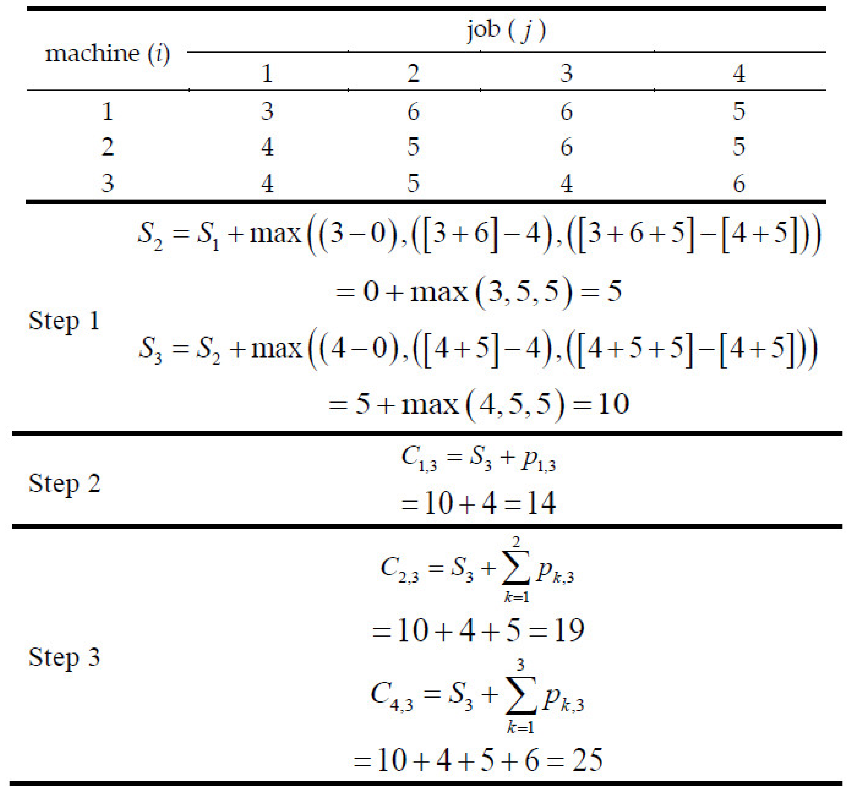
3.2. No-Idle Calculation Mechanism
To ensure that there is zero idle time throughout the production process, one should regulate each machine’s first job’s commencement. For this purpose, each machine’s start time, , is defined in:
where represents the processing time of the job assigned to the position of the sequence vector on machine . determines the start time on the previous machine. Once the start time of every machine is known, the completion time of the first job on the machine can be calculated using:
where it equals the summation of the corresponding start time of the machine and the processing time of the first job in the job sequence vector, . Next, the completion time of the job assigned to the position of the sequence vector , which is processed on the machine , is defined in:
where is equal to the completion time of job position in of job sequence vector on machine , , plus the processing time of the job positioned in , . Finally, the makespan value is calculated using:
where represents the completion time of the last job in sequence vector , which is processed on the last machine. Therefore, . An illustrative example is provided in Figure 1 to clarify the computational steps of calculating the completion time in the no-idle flowshop.
3.3. Solution Algorithm
The IG algorithm was introduced by Ruiz and Stützle [52] to solve permutation flowshops. The computational procedure of IG is inspired by human behavior when wanting a lot more of something in a greedy manner. The successful track record of the IG algorithms in solving flowshop problems inspired us to extend it for solving the problem. The pseudocode of the HIG algorithm is provided in Figure 2, followed by the details on the major computational elements. It is worthwhile mentioning that the proposed modifications are adjustable and can be effectively adapted for other application areas.
3.3.1. Solution Initialization and Decoding
Solutions are decoded as a permutation of numbers, each of which represent a job, with the processing sequence being similar on machines. Taking the job sequence as an example, the solution is symbolized by a vector, , where six jobs should be processed following the specified order on every machine. To generate the initial solution, the well-known constructive heuristic algorithm introduced by Nawaz, Enscore, Ham (NEH; [53]), which is known as one of the best constructive heuristics for solution initialization of the flowshop problems, is preferred to random solution generation to ensure a better initial approximation. The NEH considers average processing time as a priority rule for arranging the jobs. The destruction and construction module presented in the next sub-section uses the outcomes of NEH to improve the solution quality.
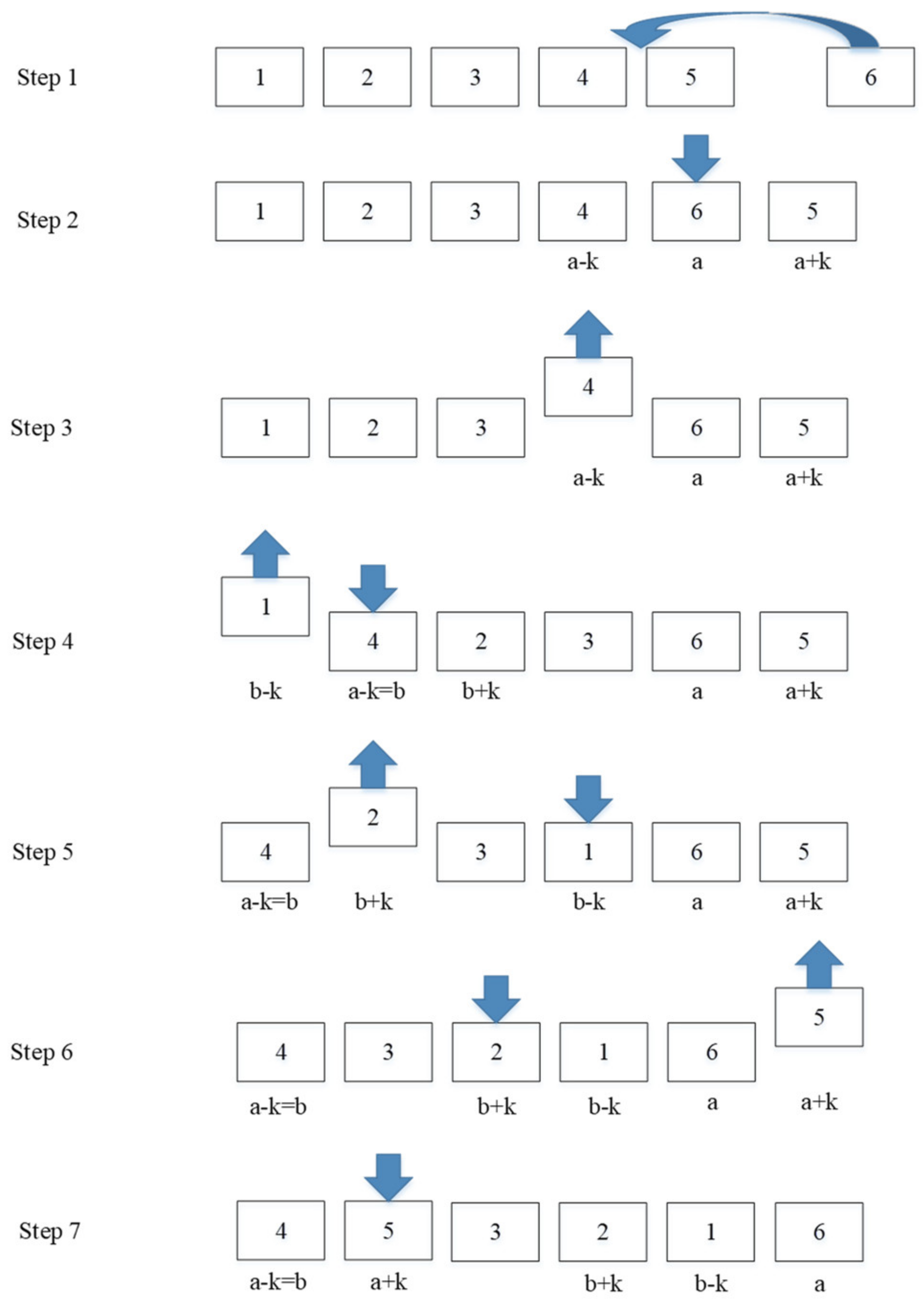
3.3.2. Destruction and Construction Methods
This study applies a random destruction method with no limits to facilitate a greater level of disturbance in the search procedure. The randomly extracted jobs, which equals the destruction count (), will then be saved in a separate array to be considered in the construction procedure. A customized construction method for sorting and inserting the removed jobs is developed to improve the effectiveness of the search procedure while ensuring the feasibility of the resulting new solution. This approach is explained below with an illustrative example of this procedure provided in Figure 3.
- Step 1. Remove the last job from and name it .
- Step 2. Insert into before the last job. Name the jobs before and after as and , respectively.
- Step 3. Remove job and rename it to .
- Step 4. Insert next to the first job in and name the jobs before and after as and , respectively.
- Step 5. Insert right before .
- Step 6. Select and move it to the position before .
- Step 7. Select and move it to the position after .
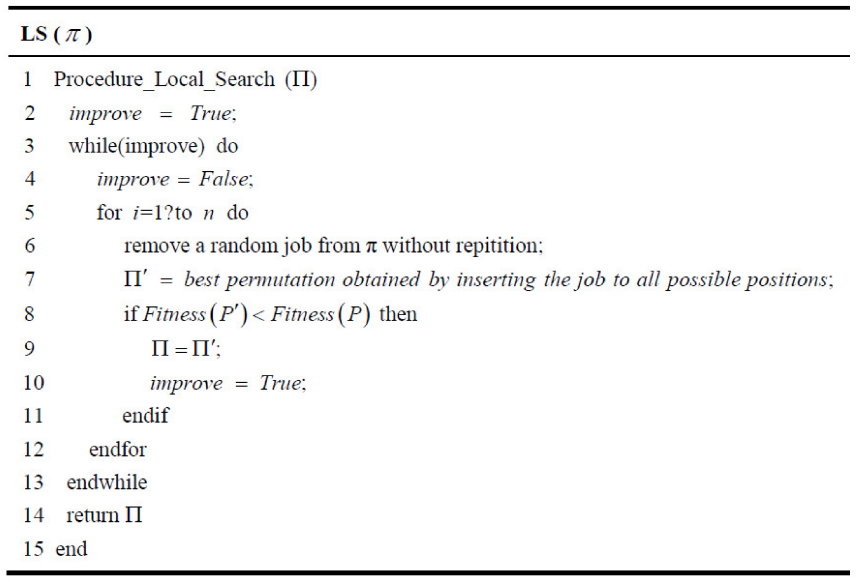
3.3.3. Local Search Method
After a new solution has resulted from the iterative and greedy construction procedure, a local search mechanism should be applied to search for further improvements. For this purpose, a pre-determined number of non-repetitive random job extraction and insertion, named as the local search count (), is used to find fitter solutions. If there is an improvement as a result of applying the local search procedure, the procedure will be continued; otherwise, it will be terminated. The pseudocode of the local search procedure is provided in Figure 4.
3.3.4. Acceptance and Stopping Conditions
Once the current best solution () and the new solution () are known, the search algorithm should determine if there is an improvement in the fitness value. If the new solution is of better quality than the current best solution, i.e., a smaller weighted sum of the total flowtime and makespan values has resulted, the new solution becomes the current-best solution, . Otherwise, a mechanism is required to decide whether or not to accept a new solution that is worse or similar to the current best solution.
Inspired by the Simulated Annealing algorithm [54], the cooling mechanism is used to regulate the acceptance condition. In the approach suggested by Ruiz and Stützle [52], the fitness values associated with the current and best solutions are considered to calculate the relative change in the solution quality, i.e., . Given and the initial temperature, , as the algorithm parameter, the current temperature decreases proportionately to the cooling coefficient, i.e., , where is the cooling rate. Finally, the acceptance probability, calculated using should be compared with a random number to determine whether to accept a poor-performing solution. This mechanism is particularly useful to avoid premature convergence and getting trapped in the local optima. Unchanged fitness value, i.e., , for a certain number of iterations, signals the termination of the algorithm. The algorithm terminates when the current best solution remains do not improve for a certain number of iterations.
4. Results
This section begins with an elaboration on the configuration of the test bank and the algorithm calibration experiment. Numerical results and statistical analysis are then provided to compare the HIG performance with Hybrid Tabu Search (HTS; [25]). It consists of short- and long-term phases, with the short-term phase focusing on a local search and the long-term phase improving concentration and diversification and help escape the local best solutions. HTS applies the NEH [53] for solution initialization, and the ‘swap’ and ‘insert’ moves as the disturbance mechanism. Besides, three other variants of IG, denoted by the IG1, IG2, and IG3 algorithms, are included to enrich the numerical experiments and provide insights into the impact of various computational elements in solving the problem. It helps explore what element of the proposed extension contributes most to the possible breakthrough. IG1 and IG2 apply the basic construction method, while IG3 uses the customized construction method developed in our study. On the other hand, IG1 and IG3 do not have a local search mechanism, while IG2 applies a perturbation mechanism similar to HIG. All the algorithms are coded and compiled using a personal computer with the following specs; Intel (R) Core (TM) i7 CPU 3.4 GHz, 8 GB RAM, and Windows 7 operating system.
The widely-used scheduling dataset developed by Tillard [55] is used to benchmark HIG against the best-performing algorithms in the literature developed to solve the problem. This dataset consists of 12 job/machine combinations considering three configuration groups: (1) jobs and machines; (2) jobs and machines; (3) jobs and machines. Ten distinct instances for each combination make a total of 120 instances for the final experiments.
The calibration experiment is conducted in two phases using random test instances. First, the best configuration is determined considering a limited set of alternatives. Next, the set of parameters adjacent to the selected configuration in the first phase will be explored to check if a better combination of parameters can be found. For this purpose, the Relative Percentage Deviation (RPD) shown in Equation (13) is considered to compare the resulting fitness values where smaller values are preferred, and 0 demonstrates the best solution. In this equation, refers to the fitness value obtained by each of the solution algorithms and is the best result.
Random instances are used to determine the parameters of the IG1, IG2, IG3, and HIG algorithms. The calibration test results are summarized in Table 2 for these algorithms. On this basis, the algorithm parameters are set to , , and to conduct the final experiments. To ensure a fair comparison, a termination condition similar to that of the HTS algorithm, which is applied by Ren et al. [25], is considered. That is, the algorithm terminates when the current best solution remains unchanged for 100 consecutive iterations.
Considering the calibrated parameter values and an equal importance weight () within a priori performance articulation scheme, the best-found solutions of the instances solved using HTS [25] are compared to those of the HTS, IG1, IG2, and IG1 algorithms. The results are summarized in Table 3 and Table 4. Except for the instance with 20 machines and 10 jobs (), where HTS performs slightly better than HIG, the rest of the best solutions are yielded by HIG.
We first analyze the results considering various workloads and operating scales. Considering different numbers of jobs in the first set of instances, Table 3 shows that HIG performs better than HTS. The difference in performance becomes more significant with an increase in the workload. The IG2 algorithm is also superior to the HTS, considering the first set of test instances, showing that integrating the local search mechanism contributes significantly to the success of the developed algorithm. The solutions obtained by the IG1, IG2, IG3, and HIG algorithms across all test instances are then compared separately in Table 4, considering all test instances where HIG yields the best results in all cases.
In an overall analysis, Table 5 and Table 6 provide the Average Relative Percentage Deviation (ARPD) values for different workloads and machines, respectively. The RPD analysis shows the overall impact of the number of machinery and workload on the performance of the algorithm. It is evident that HIG obtains meaningfully better solutions than the HTS, IG1, IG2, and IG3 algorithms when solving the problem across different operational situations. Given the RPD analysis, it is expected that HIG’s superiority to the current-best-performing algorithm, HTS, will be even more significant for industry-scale applications.
A statistical test is conducted to check whether the resulting improvement in the best-found solutions is significant. The null hypothesis is that the HIG algorithm does not outperform the HTS algorithm when solving the problem. The t-test results are summarized in Table 7. Considering 120 test instances, the p-value is supportive of rejecting the null hypothesis. That is, with 95 percent of confidence, we can claim that HIG is superior to the current-best-performing algorithm in the literature of BNIPFSP, i.e., the HTS algorithm. It is also observed that the proposed extension shows a significant improvement in the performance of the algorithm when compared to all three variants of the IGs.
As a final step to the numerical analysis, the best-found solutions to all 120 test instances are recorded in Appendix B. The updated values are highlighted in bold font. Notably, 119 out of 120 best-found solutions are yielded by the HIG algorithm. The resulting values can be used in future studies to benchmark the prospect solution algorithms for solving the problem.
5. Conclusions
Energy efficiency in the production sector requires well-informed operations management decisions in addition to the use of modern equipment, smart lighting and control systems, and the standard construction of facilities. Production scheduling is a prime example of planning tools that facilitate the successful implementation of green initiatives for reducing the carbon footprint. This study contributes to the energy-efficient production scheduling literature developing a mathematical model and a solution algorithm to address the gap identified in the comprehensive literature review. Extensive numerical analysis using a well-known dataset showed that almost all of the best-found solutions are yielded by the HIG algorithm. The statistical test of significance confirmed that HIG performs significantly better than the benchmark algorithm when solving the problem.
Despite its effectiveness in solving the BNIPFSPs, the proposed solution algorithm is limited in that it applies a priori preference articulation approach for reconciliation of the makespan and total flowtime. To address this limitation, the following directions can be pursued. First, one can extend the Iterated Greedy algorithm to work with the Pareto Front approach to provide a comprehensive set of optimum solutions and trade-offs. Second, other multi-objective optimization algorithms can be adapted to solve this intractable scheduling extension. The third suggestion for future research includes adopting the Concept of Stratification and Incremental Enlargement to solve the problem’s dynamic variant. In doing so, one can also account for operational parameter uncertainties and the possibility of rejecting a job or partially accepting a batch of jobs. Finally, the no-idle setting needs more attention in other production settings to contribute to energy efficiency literature.
Author Contributions
C.-Y.C.: Conceptualization, Methodology, Software. S.-W.L.: Conceptualization, Methodology, Software, Funding acquisition. P.P.: Investigation, Writing—Original draft, Writing—Revision. K.-C.Y.: Supervision, Conceptualization, Methodology. Y.-Z.L.: Formal analysis. All authors have read and agreed to the published version of the manuscript.
Funding
This research was partially supported by the Ministry of Science and Technology, Taiwan, under Grant MOST 109-2221-E-027-073/Most-109-2410-H-182-009-MY3, and in part by the Linkou Chang Gung Memorial Hospital under Grant BMRPA19.
Institutional Review Board Statement
Not applicable.
Informed Consent Statement
Not applicable.
Data Availability Statement
Not applicable.
Conflicts of Interest
The authors declare no conflict of interest.
Appendix A

Table A1.
Summary of the No-Idle Flowshop Scheduling Literature.
| Title | Authors (Year) | Publication | Scheduling Extension | Objective Function |
|---|---|---|---|---|
| Note: On the Two-Machine No-Idle Flowshop Problem | Cepek et al. (2000) | Naval Research Logistics | No-idle permutation flowshop | Total completion time |
| Flowshop/no-idle scheduling to minimize the mean flowtime | Narain and Bagga (2005) | Australia and New Zealand Industrial and Applied Mathematics (ANZIAM) | No-idle permutation flowshop | Average flowtime |
| No-wait flexible flowshop scheduling with no-idle machines | Wang et al. (2005) | Operations Research Letters | No-wait flexible flowshop with no-idle machines | Makespan |
| A differential evolution algorithm for the no-idle flowshop scheduling problem with total tardiness criterion | Tasgetiren et al. (2011) | International Journal of Production Research | No-idle permutation flowshop | Total tardiness |
| Tabu search algorithm for no-idle flowshop scheduling problems | Ren et al. (2010) | Computer Engineering and Design | No-idle permutation flowshop | Makespan |
| A DE Based Variable Iterated Greedy Algorithm for the No-Idle Permutation Flowshop Scheduling Problem with Total Flowtime Criterion | Tasgetiren et al. (2011) | Conference | No-idle permutation flowshop | Total flowtime |
| Hybrid Tabu Search Algorithm for bi-criteria no-idle permutation flow shop scheduling problem | Ren et al. (2011) | Conference | Bi-objective no-idle permutation flowshop | Makespan and total flowtime |
| A new heuristic method for minimizing the makespan in a no-idle permutation flowshop | Nagano & Branco (2012) | Conference | No-idle permutation flowshop | Makespan |
| A discrete artificial bee colony algorithm for the no-idle permutation flowshop scheduling problem with the total tardiness criterion | Tasgetiren et al. (2013b) | Applied Mathematical Modelling | No-idle permutation flowshop | Total tardiness |
| A variable iterated greedy algorithm with differential evolution for the no-idle permutation flowshop scheduling problem | Tasgetiren et al. (2013a) | Computers & Operations Research | No-idle permutation flowshop | Makespan |
| Metaheuristics for the no-idle permutation flowshop scheduling problem | Büyükdağlı (2013) | Thesis | No-idle permutation flowshop | - |
| An effective iterated greedy algorithm for the mixed no-idle permutation flowshop scheduling problem | Pan and Ruiz (2014) | OMEGA | Mixed no-idle permutation flowshop | Makespan |
| Research on no-idle permutation flowshop scheduling with time-dependent learning effect and deteriorating jobs | Lu (2016) | Applied Mathematical Modelling | No-idle permutation flowshop scheduling with time-dependent learning effect and deteriorating jobs | Makespan |
| Heuristics for the mixed no-idle flowshop with sequence-dependent setup times and total flowtime criterion | Rossi and Nagano (2019a) | Expert Systems with Applications | Mixed no-idle permutation flowshop with SDST | Total flowtime |
| Heuristics for the mixed no-idle flowshop with sequence-dependent setup times | Rossi and Nagano (2019b) | Journal of the Operational Research Society | Mixed no-idle permutation flowshop with SDST | Makespan |
| High-performing heuristics to minimize flowtime in no-idle permutation flowshop | Nagano et al. (2019) | Engineering Optimization | No-idle permutation flowshop | Total flowtime |
| A Variable Iterated Local Search Algorithm for Energy-Efficient No-idle Flowshop Scheduling Problem | Tasgetiren et al. (2019) | Conference | Bi-objective no-idle permutation flowshop | Makespan and total energy consumption |
| A contribution for the mixed no-idle flowshop scheduling problem with sequence-dependent setup times: analysis and solutions procedures | Rossi (2020) | Thesis | Mixed no-idle flowshop with sequence-dependent setup times | - |
| A hybrid discrete water wave optimization algorithm for the no-idle flowshop scheduling problem with total tardiness criterion | Zhao et al. (2020) | Expert Systems with Applications | No-idle permutation flowshop | Total tardiness |
| A new iterated greedy algorithm for no-idle permutation flowshop scheduling with the total tardiness criterion | Riahi et al. (2020) | Computers & Operations Research | No-idle permutation flowshop | Total tardiness |
| Benders decomposition for the mixed no-idle permutation flowshop scheduling problem | Bektaş et al. (2020) | Journal of Scheduling | Mixed no-idle permutation flowshop | Makespan |
| Heuristics and metaheuristics for the mixed no-idle flowshop with sequence-dependent setup times and total tardiness minimization | Rossi and Nagano (2020) | Swarm and Evolutionary Computation | Mixed no-idle permutation flowshop with sequence-dependent setup times | Total tardiness |
| A Novel General Variable Neighborhood Search through Q-Learning for No-Idle Flowshop Scheduling | Oztop et al. (2020) | Conference | No-idle permutation flowshop | Makespan |
| Automatic design of hybrid stochastic local search algorithms for permutation flowshop problems with additional constraints | Pagnozzi and Stützle (2021) | Operations Research Perspectives | No-idle permutation flowshop | Makespan |
| A cooperative water wave optimization algorithm with reinforcement learning for the distributed assembly no-idle flowshop scheduling problem | Zhao et al. (2021) | Computers & Industrial Engineering | Distributed assembly no-idle flow-shop scheduling problem | Maximum assembly completion time |
Appendix B
Table A2.
Best-Found Solutions (BFS) across All Test Instances (Updates in Bold).
| Inst. | BFS | Inst. | BFS | Inst. | BFS | Inst. | BFS | Inst. | BFS | |||||
|---|---|---|---|---|---|---|---|---|---|---|---|---|---|---|
| 1 | 9324.5 | 2 | 8768.5 | 3 | 9004.0 | 4 | 9201.0 | 5 | 9840.0 | |||||
| 17,456.0 | 15,359.5 | 15,311.0 | 15,060.5 | 12,932.0 | ||||||||||
| 29,148.5 | 27,458.5 | 29,330.0 | 27,500.5 | 30,123.5 | ||||||||||
| 45,895.5 | 40,849.5 | 39,540.0 | 40,900.0 | 46,931.0 | ||||||||||
| 57,582.5 | 56,394.5 | 55,894.5 | 60,125.5 | 53,752.0 | ||||||||||
| 105,555.0 | 119,208.5 | 95984.5 | 113,445.5 | 97,119.0 | ||||||||||
| 155,420.0 | 134,879.0 | 133,638.0 | 133,875.5 | 147,159.0 | ||||||||||
| 201,117.5 | 178,403.0 | 212,533.0 | 191,444.5 | 195,680.5 | ||||||||||
| 324,920.5 | 297,506.0 | 310,170.5 | 345,987.0 | 355,364.0 | ||||||||||
| 656,480.0 | 752,145.0 | 729,595.0 | 618,158.0 | 667,624.5 | ||||||||||
| 989,277.5 | 962,653.5 | 944,299.5 | 903,733.0 | 987,579.5 | ||||||||||
| 4,448,496.5 | 4,550,718 | 4,927,311 | 4,443,889 | 485,7293 | ||||||||||
| 6 | 9974.0 | 7 | 7746.5 | 8 | 8809.5 | 9 | 9435.5 | 10 | 8213.0 | |||||
| 15,218.5 | 13,795.0 | 15,206.0 | 15,190.0 | 14,449.5 | ||||||||||
| 30,508.0 | 28,473.5 | 29,676.5 | 29,177.0 | 32,824.0 | ||||||||||
| 40,562.5 | 43,979.0 | 41,450.0 | 39,433.0 | 40,033.0 | ||||||||||
| 67,395.5 | 61,381.0 | 65,124.5 | 59,999.0 | 61,566.0 | ||||||||||
| 116,283.0 | 113,469.0 | 102,066.0 | 104,491.5 | 111,647.5 | ||||||||||
| 135,117.0 | 158,846.0 | 130,140.5 | 138,971.0 | 139,377.0 | ||||||||||
| 198,459.5 | 216,278.5 | 214,725.5 | 21,8945.0 | 201,118.0 | ||||||||||
| 294,212.0 | 310,486.0 | 300,453.0 | 321,981.0 | 301,118.0 | ||||||||||
| 698,950.5 | 6,123,41.5 | 705,257.0 | 601,637.0 | 700,784.5 | ||||||||||
| 976,708.0 | 1,025,032 | 1,003,762 | 919,347.5 | 914,365.5 | ||||||||||
| 446,0524 | 4,829,931 | 4,979,367 | 4,414,894 | 489,4606 |
References
- Zhu, Z.-S.; Liao, H.; Cao, H.-S.; Wang, L.; Wei, Y.-M.; Yan, J. The differences of carbon intensity reduction rate across 89 countries in recent three decades. Appl. Energy 2014, 113, 808–815. [Google Scholar] [CrossRef]
- Sutherland, B.R. Tax Carbon Emissions and Credit Removal. Joule 2019, 3, 2071–2073. [Google Scholar] [CrossRef]
- Agency, I.E. Tracking Industrial Energy Efficiency and CO2 Emissions; OECD: Paris, France, 2007; ISBN 9789264030169. [Google Scholar]
- Pourhejazy, P.; Kwon, O.K.; Lim, H. Integrating Sustainability into the Optimization of Fuel Logistics Networks. KSCE J. Civ. Eng. 2019, 23, 1369–1383. [Google Scholar] [CrossRef]
- Zhang, H.C.; Kuo, T.C.; Lu, H.; Huang, S.H. Environmentally conscious design and manufacturing: A state-of-the-art survey. J. Manuf. Syst. 1997, 16, 352–371. [Google Scholar] [CrossRef]
- Pourhejazy, P.; Kwon, O.K. A Practical Review of Green Supply Chain Management: Disciplines and Best Practices. J. Int. Logist. Trade 2016, 14, 156–164. [Google Scholar] [CrossRef]
- Peng, C.; Peng, T.; Zhang, Y.; Tang, R.; Hu, L. Minimising non-processing energy consumption and tardiness fines in a mixed-flow shop. Energies 2018, 11, 3382. [Google Scholar] [CrossRef] [Green Version]
- Cheng, C.-Y.; Pourhejazy, P.; Ying, K.-C.; Lin, C.-F. Unsupervised Learning-based Artificial Bee Colony for minimizing non-value-adding operations. Appl. Soft Comput. 2021, 105, 107280. [Google Scholar] [CrossRef]
- Wu, X.; Sun, Y. A green scheduling algorithm for flexible job shop with energy-saving measures. J. Clean. Prod. 2018, 172, 3249–3264. [Google Scholar] [CrossRef]
- Piroozfard, H.; Wong, K.Y.; Wong, W.P. Minimizing total carbon footprint and total late work criterion in flexible job shop scheduling by using an improved multi-objective genetic algorithm. Resour. Conserv. Recycl. 2018, 128, 267–283. [Google Scholar] [CrossRef]
- Zheng, X.-L.; Wang, L. A collaborative multiobjective fruit fly optimization algorithm for the resource constrained unrelated parallel machine green scheduling problem. IEEE Trans. Syst. Man Cybern. Syst. 2016, 48, 790–800. [Google Scholar] [CrossRef]
- Safarzadeh, H.; Niaki, S.T.A. Bi-objective green scheduling in uniform parallel machine environments. J. Clean. Prod. 2019, 217, 559–572. [Google Scholar] [CrossRef]
- Mansouri, S.A.; Aktas, E.; Besikci, U. Green scheduling of a two-machine flowshop: Trade-off between makespan and energy consumption. Eur. J. Oper. Res. 2016, 248, 772–788. [Google Scholar] [CrossRef] [Green Version]
- Zhang, B.; Pan, Q.; Gao, L.; Li, X.; Meng, L.; Peng, K. A multiobjective evolutionary algorithm based on decomposition for hybrid flowshop green scheduling problem. Comput. Ind. Eng. 2019, 136, 325–344. [Google Scholar] [CrossRef]
- Cota, L.P.; Coelho, V.N.; Guimarães, F.G.; Souza, M.J.F. Bi-criteria formulation for green scheduling with unrelated parallel machines with sequence-dependent setup times. Int. Trans. Oper. Res. 2021, 28, 996–1017. [Google Scholar] [CrossRef]
- Jiang, T.; Zhang, C.; Sun, Q.-M. Green job shop scheduling problem with discrete whale optimization algorithm. IEEE Access 2019, 7, 43153–43166. [Google Scholar] [CrossRef]
- Aghelinejad, M.; Ouazene, Y.; Yalaoui, A. Complexity analysis of energy-efficient single machine scheduling problems. Oper. Res. Perspect. 2019, 6, 100105. [Google Scholar] [CrossRef]
- Li, K.; Zhang, X.; Leung, J.Y.-T.; Yang, S.-L. Parallel machine scheduling problems in green manufacturing industry. J. Manuf. Syst. 2016, 38, 98–106. [Google Scholar] [CrossRef]
- Niu, S.; Song, S.; Chiong, R. A Distributionally Robust Scheduling Approach for Uncertain Steelmaking and Continuous Casting Processes. IEEE Trans. Syst. Man Cybern. Syst. 2021. [Google Scholar] [CrossRef]
- Bektaş, T.; Hamzadayı, A.; Ruiz, R. Benders decomposition for the mixed no-idle permutation flowshop scheduling problem. J. Sched. 2020, 23, 513–523. [Google Scholar] [CrossRef] [Green Version]
- Ding, J.-Y.; Song, S.; Gupta, J.N.D.; Wang, C.; Zhang, R.; Wu, C. New block properties for flowshop scheduling with blocking and their application in an iterated greedy algorithm. Int. J. Prod. Res. 2016, 54, 4759–4772. [Google Scholar] [CrossRef]
- Foumani, M.; Smith-Miles, K. The impact of various carbon reduction policies on green flowshop scheduling. Appl. Energy 2019, 249, 300–315. [Google Scholar] [CrossRef]
- Graham, R.L.; Lawler, E.L.; Lenstra, J.K.; Kan, A.H.G.R. Optimization and Approximation in Deterministic Sequencing and Scheduling: A Survey. In Annals of Discrete Mathematics; Elsevier: Amsterdam, The Netherlands, 1979; Volume 5, pp. 287–326. [Google Scholar]
- Tasgetiren, M.F.; Pan, Q.-K.; Wang, L.; Chen, A.H.-L. A DE based variable iterated greedy algorithm for the no-idle permutation flowshop scheduling problem with total flowtime criterion. In Proceedings of the International Conference on Intelligent Computing, Zhengzhou, China, 11–14 August 2011; pp. 83–90. [Google Scholar]
- Ren, W.-J.; Duan, J.-H.; Zhang, F.; Han, H.; Zhang, M. Hybrid Tabu Search Algorithm for bi-criteria No-idle permutation flow shop scheduling problem. In Proceedings of the 2011 Chinese Control and Decision Conference (CCDC), Mianyang, China, 23–25 May 2011; pp. 1699–1702. [Google Scholar]
- Nagano, M.S.; Branco, F.J.C. A new heuristic method for minimizing the makespan in a no-idle permutation flowshop. In Proceedings of the Simposio Brasileiro de Pesquisa Operacional, Rio de Janeiro, Brazil, 24–28 September 2012. [Google Scholar]
- Fatih Tasgetiren, M.; Öztop, H.; Gao, L.; Pan, Q.K.; Li, X. A Variable Iterated Local Search Algorithm for Energy-Efficient No-idle Flowshop Scheduling Problem. Procedia Manuf. 2019, 39, 1185–1193. [Google Scholar] [CrossRef]
- Oztop, H.; Tasgetiren, M.F.; Kandiller, L.; Pan, Q.K. A Novel General Variable Neighborhood Search through Q-Learning for No-Idle Flowshop Scheduling. In Proceedings of the 2020 IEEE Congress on Evolutionary Computation (CEC), Glasgow, UK, 19–24 July 2020. [Google Scholar] [CrossRef]
- Rossi, F.L. A Contribution for the Mixed No-Idle Flowshop Scheduling Problem with Sequence-Dependent Setup Times: Analysis and Solutions Procedures. Ph.D. Thesis, Universidade de São Paulo, São Paulo, Brazil, 2019. [Google Scholar]
- Buyukdagli, O. Metaheuristics for the No-Idle Permutation Flowshop Scheduling Problem. Master Thesis, Yasar University, Bornova, Turkey, 2013. [Google Scholar]
- Ribas, I.; Leisten, R.; Framiñan, J.M. Review and classification of hybrid flow shop scheduling problems from a production system and a solutions procedure perspective. Comput. Oper. Res. 2010, 37, 1439–1454. [Google Scholar] [CrossRef]
- Neufeld, J.S.; Gupta, J.N.D.; Buscher, U. A comprehensive review of flowshop group scheduling literature. Comput. Oper. Res. 2016, 70, 56–74. [Google Scholar] [CrossRef]
- Cepek, O.; Okada, M.; Vlach, M. Minimizing total completion time in a two-machine no-idle flowshop. Res. Rep. 1998, 98, 1–23. [Google Scholar]
- Čepek, O.; Okada, M.; Vlach, M. Note: On the Two-Machine No-Idle Flowshop Problem. Nav. Res. Logist. 2000, 47, 353–358. [Google Scholar] [CrossRef]
- Narain, L.; Bagga, P.C. Flowshop/no-idle scheduling to minimise the mean flowtime. ANZIAM J. 2005, 47, 265–275. [Google Scholar] [CrossRef] [Green Version]
- Wang, Z.; Xing, W.; Bai, F. No-wait flexible flowshop scheduling with no-idle machines. Oper. Res. Lett. 2005, 33, 609–614. [Google Scholar] [CrossRef]
- Tasgetiren, M.F.; Pan, Q.K.; Suganthan, P.N.; Jin Chua, T. A differential evolution algorithm for the no-idle flowshop scheduling problem with total tardiness criterion. Int. J. Prod. Res. 2011, 49, 5033–5050. [Google Scholar] [CrossRef]
- Fatih Tasgetiren, M.; Pan, Q.K.; Suganthan, P.N.; Oner, A. A discrete artificial bee colony algorithm for the no-idle permutation flowshop scheduling problem with the total tardiness criterion. Appl. Math. Model. 2013, 37, 6758–6779. [Google Scholar] [CrossRef]
- Ren, W.-J.; Pan, Q.-K.; Han, H.-Y. Tabu search algorithm for no-idle flowshop scheduling problems. Comput. Eng. Des. 2010, 31, 5071–5074. [Google Scholar]
- Fatih Tasgetiren, M.; Pan, Q.K.; Suganthan, P.N.; Buyukdagli, O. A variable iterated greedy algorithm with differential evolution for the no-idle permutation flowshop scheduling problem. Comput. Oper. Res. 2013, 40, 1729–1743. [Google Scholar] [CrossRef]
- Lu, Y.Y. Research on no-idle permutation flowshop scheduling with time-dependent learning effect and deteriorating jobs. Appl. Math. Model. 2016, 40, 3447–3450. [Google Scholar] [CrossRef]
- Pagnozzi, F.; Stützle, T. Automatic design of hybrid stochastic local search algorithms for permutation flowshop problems with additional constraints. Oper. Res. Perspect. 2021, 8, 100180. [Google Scholar]
- Pan, Q.-K.; Ruiz, R. An effective iterated greedy algorithm for the mixed no-idle permutation flowshop scheduling problem. Omega 2014, 44, 41–50. [Google Scholar] [CrossRef] [Green Version]
- Rossi, F.L.; Nagano, M.S. Heuristics for the mixed no-idle flowshop with sequence-dependent setup times and total flowtime criterion. Expert Syst. Appl. 2019, 125, 40–54. [Google Scholar] [CrossRef]
- Rossi, F.L.; Nagano, M.S. Heuristics and metaheuristics for the mixed no-idle flowshop with sequence-dependent setup times and total tardiness minimisation. Swarm Evol. Comput. 2020, 55, 100689. [Google Scholar] [CrossRef]
- Rossi, F.L.; Nagano, M.S. Heuristics for the mixed no-idle flowshop with sequence-dependent setup times. J. Oper. Res. Soc. 2019, 1–27. [Google Scholar] [CrossRef]
- Nagano, M.S.; Rossi, F.L.; Martarelli, N.J. High-performing heuristics to minimize flowtime in no-idle permutation flowshop. Eng. Optim. 2019, 51, 185–198. [Google Scholar] [CrossRef]
- Zhao, F.; Zhang, L.; Zhang, Y.; Ma, W.; Zhang, C.; Song, H. A hybrid discrete water wave optimization algorithm for the no-idle flowshop scheduling problem with total tardiness criterion. Expert Syst. Appl. 2020, 146, 113166. [Google Scholar] [CrossRef]
- Riahi, V.; Chiong, R.; Zhang, Y. A new iterated greedy algorithm for no-idle permutation flowshop scheduling with the total tardiness criterion. Comput. Oper. Res. 2020, 117, 104839. [Google Scholar] [CrossRef]
- Zhao, F.; Zhang, L.; Cao, J.; Tang, J. A cooperative water wave optimization algorithm with reinforcement learning for the distributed assembly no-idle flowshop scheduling problem. Comput. Ind. Eng. 2021, 153, 107082. [Google Scholar] [CrossRef]
- Ruiz, R.; Vallada, E.; Fernandez-Martinez, C. Scheduling in flowshops with no-idle machines. In Computational Intelligence in Flow Shop and Job Shop Scheduling; Springer: Berlin/Heidelberg, Germany, 2009; pp. 21–51. [Google Scholar]
- Ruiz, R.; Stützle, T. A simple and effective iterated greedy algorithm for the permutation flowshop scheduling problem. Eur. J. Oper. Res. 2007, 177, 2033–2049. [Google Scholar] [CrossRef]
- Nawaz, M.; Enscore, E.E., Jr.; Ham, I. A heuristic algorithm for the m-machine, n-job flow-shop sequencing problem. Omega 1983, 11, 91–95. [Google Scholar] [CrossRef]
- Osman, I.; Potts, C. Simulated annealing for permutation flow-shop scheduling. Omega 1989, 17, 551–557. [Google Scholar] [CrossRef]
- Taillard, E. Benchmarks for basic scheduling problems. Eur. J. Oper. Res. 1993, 64, 278–285. [Google Scholar] [CrossRef]
Figure 1.
Illustrative example on the calculation of the completion time in no-idle flowshops.

Figure 2.
Pseudocode of the Hybrid Iterated Greedy.

Figure 3.
The customized construction method for no-idle permutation flowshops considering .

Figure 4.
Pseudocode of the local search procedure.

Table 1.
Mathematical notations.
| Symbol | Definition |
|---|---|
| Number of jobs at hand | |
| Number of available machines | |
| Job tag and its position index in the sequence vector, i.e., ; | |
| Machine tag; | |
| Processing time of job on machine | |
| Binary decision variable, if job is positioned at index of the vector; , otherwise | |
| Integer decision variable, the completion time of the job assigned to position on machine | |
| The total flowtime of job |
Table 2.
Calibration results analysis (best in bold).
| Algorithm | Parameter | Phase I | Phase II | ||||
|---|---|---|---|---|---|---|---|
| IG1 | I | II | III | I | IV | V | |
| d | 2 | 4 | 6 | 2 | 1 | 3 | |
| γ | 20 | 40 | 60 | 20 | 10 | 30 | |
| δ | 0.9 | 0.8 | 0.7 | 0.9 | 0.95 | 0.85 | |
| ARPD | 0.56 | 1.35 | 1.61 | 0.78 | 2.78 | 1.26 | |
| IG2 | I | II | III | I | IV | V | |
| d | 2 | 4 | 6 | 2 | 1 | 3 | |
| γ | 20 | 40 | 60 | 20 | 10 | 30 | |
| δ | 0.9 | 0.8 | 0.7 | 0.9 | 0.95 | 0.85 | |
| ARPD | 0.48 | 0.65 | 0.78 | 0.68 | 0.90 | 1.15 | |
| IG3 | I | II | III | I | IV | V | |
| d | 2 | 4 | 6 | 2 | 1 | 3 | |
| γ | 20 | 40 | 60 | 20 | 10 | 30 | |
| 0.9 | 0.8 | 0.7 | 0.9 | 0.95 | 0.85 | ||
| ARPD | 0.32 | 0.99 | 1.02 | 0.38 | 3.92 | 0.88 | |
| HIG | I | II | III | I | IV | V | |
| d | 2 | 4 | 6 | 2 | 1 | 3 | |
| γ | 20 | 40 | 60 | 20 | 10 | 30 | |
| δ | 0.9 | 0.8 | 0.7 | 0.9 | 0.95 | 0.85 | |
| ARPD | 0.33 | 0.48 | 0.87 | 0.44 | 4.99 | 0.49 | |
Table 3.
Best-found solutions considering the first set of test instances (best in bold).
| Instance (m × n) | HTS | IG1 | IG2 | IG3 | HIG |
|---|---|---|---|---|---|
| 9437.0 | 9549.5 | 9401.0 | 9566.5 | 9324.5 | |
| 17,456.0 | 17,716.5 | 17,616.5 | 17,539.0 | 17,472.5 | |
| 29,319.0 | 29,412.5 | 29,149.5 | 29,724.5 | 29,148.5 | |
| 47,719.0 | 46,597.0 | 46,717.5 | 47,199.5 | 45,895.5 | |
| 58,610.0 | 61,247.0 | 58,375.5 | 58,445.0 | 57,582.5 | |
| 107,007.0 | 110,308.0 | 105,657.0 | 108,775.5 | 105,555.0 | |
| 160,401.5 | 162,367.0 | 157,927.0 | 158,705.5 | 155,420.0 | |
| 214,438.5 | 206,815.5 | 202,818.0 | 207,382.5 | 201,117.5 | |
| 337,888.5 | 335,717.0 | 330,472.0 | 330,243.5 | 324,920.5 | |
| 685,369.5 | 690,565.5 | 657,372.5 | 671,582.5 | 656,480.0 | |
| 1,003,945.5 | 1,006,795.0 | 991,009.0 | 1,011,902.5 | 989,277.5 | |
| 4,456,166.0 | 4,540,516.5 | 4,449,380.0 | 4,494,197.5 | 4,448,496.5 |
Table 4.
Best-found solutions across all test instances (updates in bold).
| Instance (m × n) | IG1 | IG2 | IG3 | HIG |
|---|---|---|---|---|
| 9239.05 | 9088.05 | 9111.90 | 9031.65 | |
| 15,238.65 | 15,054.10 | 15,065.25 | 14,999.45 | |
| 29,966.20 | 29,591.90 | 29,628.70 | 29,422.00 | |
| 43,076.70 | 42,166.05 | 42,448.70 | 41,957.35 | |
| 62,506.85 | 60,375.95 | 60,962.05 | 59,921.50 | |
| 111,451.80 | 108,472.15 | 109,087.45 | 107,926.95 | |
| 144,552.95 | 141,478.15 | 142,699.50 | 140,742.30 | |
| 209,197.70 | 204,574.05 | 207,545.50 | 203,718.20 | |
| 327,279.80 | 320,069.55 | 320,393.40 | 316,219.80 | |
| 697,101.30 | 674,801.50 | 684,276.40 | 674,297.30 | |
| 990,265.30 | 965,298.95 | 974,714.40 | 962,675.70 | |
| 4,764,325.25 | 4,687,959.00 | 4,704,317.20 | 4,680,702.80 |
Table 5.
The Relative Performance Deviation considering various workloads (best in bold).
| Workload (n) | Machinery (m) | HTS | IG1 | IG2 | IG3 | HIG |
|---|---|---|---|---|---|---|
| 20 | 5 | 1.21 | 2.41 | 0.82 | 2.60 | 0.00 |
| 10 | 0.00 | 1.49 | 0.92 | 0.48 | 0.09 | |
| 20 | 0.58 | 0.91 | 0.00 | 1.98 | 0.00 | |
| Overall | 0.60 | 1.60 | 0.58 | 1.68 | 0.03 | |
| 50 | 5 | 3.97 | 1.53 | 1.79 | 2.84 | 0.00 |
| 10 | 1.78 | 6.36 | 1.38 | 1.50 | 0.00 | |
| 20 | 1.38 | 4.50 | 0.10 | 3.05 | 0.00 | |
| Overall | 2.38 | 4.13 | 1.09 | 2.46 | 0.00 | |
| 100 | 5 | 3.21 | 4.47 | 1.61 | 2.11 | 0.00 |
| 10 | 6.62 | 2.83 | 0.85 | 3.12 | 0.00 | |
| 20 | 3.99 | 3.32 | 1.71 | 1.64 | 0.00 | |
| Overall | 4.61 | 3.54 | 1.39 | 2.29 | 0.00 | |
| 200 | 10 | 4.40 | 5.19 | 0.14 | 2.30 | 0.00 |
| 20 | 1.48 | 1.77 | 0.18 | 2.29 | 0.00 | |
| Overall | 2.94 | 3.48 | 0.16 | 2.29 | 0.00 | |
| 500 | 20 | 0.17 | 2.07 | 0.02 | 1.03 | 0.00 |
Table 6.
Average Relative Performance Deviation considering operating scale (best in bold).
| Machinery (m) | Workload (n) | HTS | IG1 | IG2 | IG3 | HIG |
|---|---|---|---|---|---|---|
| 5 | 20 | 1.21 | 2.41 | 0.82 | 2.60 | 0.00 |
| 50 | 3.97 | 1.51 | 1.79 | 2.84 | 0.00 | |
| 100 | 3.21 | 4.47 | 1.61 | 2.11 | 0.00 | |
| Overall | 2.79 | 2.80 | 1.40 | 2.51 | 0.00 | |
| 10 | 20 | 0.00 | 1.49 | 0.92 | 0.48 | 0.09 |
| 50 | 1.78 | 6.36 | 1.38 | 1.50 | 0.00 | |
| 100 | 6.62 | 2.83 | 0.85 | 3.12 | 0.00 | |
| 200 | 4.40 | 5.19 | 0.14 | 2.30 | 0.00 | |
| Overall | 3.20 | 3.97 | 0.81 | 1.84 | 0.02 | |
| 100 | 20 | 0.58 | 0.91 | 0.00 | 1.98 | 0.00 |
| 50 | 1.38 | 4.50 | 0.10 | 3.05 | 0.00 | |
| 100 | 3.99 | 3.32 | 1.71 | 1.64 | 0.00 | |
| 200 | 1.48 | 1.77 | 0.18 | 2.29 | 0.00 | |
| 500 | 0.17 | 2.07 | 0.02 | 1.03 | 0.00 | |
| Overall | 1.26 | 2.09 | 0.33 | 1.66 | 0.00 |
Table 7.
Paired t-test analysis of the performance differences under 0.95 confidence interval.
| Instance | Average | StD | DoF | T Stat | One-Tail | Two-Tail | ||
|---|---|---|---|---|---|---|---|---|
| t-Critical | p-Value | t-Critical | p-Value | |||||
| HIG Vs. HTS | 7255.58 | 8435.13 | 11 | 2.86 | 1.79 | 0.0078 | 2.20 | 0.0157 |
StD: Standard Deviation, S.E.: Standard Error of the Mean, DoF: Degree of Freedom.
Publisher’s Note: MDPI stays neutral with regard to jurisdictional claims in published maps and institutional affiliations. |
© 2021 by the authors. Licensee MDPI, Basel, Switzerland. This article is an open access article distributed under the terms and conditions of the Creative Commons Attribution (CC BY) license (https://creativecommons.org/licenses/by/4.0/).
Share and Cite
MDPI and ACS Style
Cheng, C.-Y.; Lin, S.-W.; Pourhejazy, P.; Ying, K.-C.; Lin, Y.-Z. No-Idle Flowshop Scheduling for Energy-Efficient Production: An Improved Optimization Framework. Mathematics 2021, 9, 1335. https://doi.org/10.3390/math9121335
AMA Style
Cheng C-Y, Lin S-W, Pourhejazy P, Ying K-C, Lin Y-Z. No-Idle Flowshop Scheduling for Energy-Efficient Production: An Improved Optimization Framework. Mathematics. 2021; 9(12):1335. https://doi.org/10.3390/math9121335
Chicago/Turabian StyleCheng, Chen-Yang, Shih-Wei Lin, Pourya Pourhejazy, Kuo-Ching Ying, and Yu-Zhe Lin. 2021. "No-Idle Flowshop Scheduling for Energy-Efficient Production: An Improved Optimization Framework" Mathematics 9, no. 12: 1335. https://doi.org/10.3390/math9121335
Note that from the first issue of 2016, this journal uses article numbers instead of page numbers. See further details here.