A Comparison of Discrete Schemes for Numerical Solution of Parabolic Problems with Fractional Power Elliptic Operators

Abstract

The main aim of this article is to analyze the efficiency of general solvers for parabolic problems with fractional power elliptic operators. Such discrete schemes can be used in the cases of non-constant elliptic operators, non-uniform space meshes and general space domains. The stability results are proved for all algorithms and the accuracy of obtained approximations is estimated by solving well-known test problems. A modification of the second order splitting scheme is presented, it combines the splitting method to solve locally the nonlinear subproblem and the AAA algorithm to solve the nonlocal diffusion subproblem. Results of computational experiments are presented and analyzed.

1. Introduction

In recent decades fractional differential equations proved to be important techniques for modeling diffusive type processes when an anomalous diffusion is important. A very good review on fractional calculus methods and techniques to solve differential and integro-differential equations with fractional derivatives is presented in [1,2].

Fractional derivatives are nonlocal integro-differential operators. They allow to simulate more accurately various complex physical system. From the modelling point it is very useful that fractional derivatives incorporate in a unified framework asymmetric non-Fickian transport, non-Markovian effects, including long memory effects. We will mention only a few important investigations. Applications of fractional calculus to describe generalized dynamical systems and discrete maps, non-local statistical mechanics and kinetics, dynamics of open quantum systems with non-local properties and memory are considered in [3], the analysis of fluid flow in fractal porous medium is done in [4]. The fractional calculus techniques are used intensively in quantum mechanical problems, for example a fractional generalization of the free particle problem is found, the corresponding fractional Schrödinger equation is derived in [5], analysis of statistic and dynamical systems [6]. A generalization of fractional Dirac operators and applications in deformed field theory are considered in [7]. Integral and fractional derivatives of order $(\alpha ,\beta )$ and dynamical fractional integral exponents are investigated in [8], and a useful table of some basic fractional calculus formulae derived from a modified Riemann–Liouville derivative for non-differentiable functions is presented in [9].

In this paper we restrict to one important class of problems dealing with nonlocal diffusion operators defined as fractional powers of elliptic operators. Such mathematical models describe a broad class of real-world processes. We will mention only applications in cell biology [10], models used to describe chemical and contaminant transport in heterogeneous aquifer [11], physics [12], finance [13], medicine [14], and image processing [15]. The fractional-order models appear to be more adequate than the standard models in the description of the long range interactions, memory and hereditary properties of different substances [16]. More examples are given in [17].

The fractional power of an elliptic operator $A_h^{\alpha }$ can be defined in non-unique way. In this paper we use the spectral definition (the details are given in Section 2). It is important to note, that the given spectral algorithm can be used for practical computations to solve parabolic type problems with nonlocal operator $A_h^{\alpha }$. However, this strategy is efficient only if the problem is solved in a rectangular domain, the complete set of eigenfunctions of operator $A_h$ are known in advance and FFT techniques can be applied.

Thus in the case of non-uniform space meshes and/or elliptic operators with non-constant coefficients for solution of nonlocal problems with fractional power operators alternative approaches are used. The main idea is to transform non-local problems into the local classical differential problems. Here we briefly mention the most interesting transformations, a very good review on these methods is given in [18].

First we mention a general integral representation of the solution with standard Laplacian operator [19]. After approximation of integrals by some efficient specialized quadrature formula a set of local elliptic problems is solved and an approximation of the solution of non-local problem is constructed.

A more general approach is to change the nonlocal discrete operator $A_h^{\alpha }$ by its rational approximation. A few different implementations are proposed. In the BURA method the best uniform rational approximation formula is used [20]. For the negative power of a matrix $A_h^{-\beta }$ a rational function approximating the mapping $z\to z^{-\beta }$ is constructed via a modified Remez algorithm. It should be noted that the determination of coefficients for this rational function is very sensitive to rounding errors and therefore it requires non-trivial computations.

Another very robust and accurate technique to construct rational approximations is based on the so-called AAA algorithm proposed in [21]. In this paper we will use this method widely as an essential part of three algorithms proposed to solve parabolic problems with fractional power elliptic operators.

We also mention an interesting approach when the original nonlocal fractional problem in a d-dimensional domain is transformed into a Neumann-to-Dirichlet map for a local, elliptic problem in a $d+1$-dimensional cylinder built on the original domain [22]. Efficient multilevel and tensor FEM solvers for the resulting $d+1$-dimensional problems are described in [23,24].

One more original transformation is proposed in [25], where the nonlocal problem is transformed into a classical local pseudo-parabolic problem. The accuracy and efficiency of this method is essentially improved in [26,27], where high-order modifications are proposed, including a special time grid to integrate the problem in time.

Recently many papers are devoted to solve nonstationary (parabolic) problems with fractional power elliptic operators. The proposed discrete schemes are mainly based on spectral methods and the approximation and stability analysis is done for various multidimensional problems (see [17,28,29,30] and references given therein). An original Fourier spectral exponential time differencing method is proposed in [31].

In this paper we are interested to compare general methods suited to solve nonstationary problems for elliptic operators with non-constant coefficients, in non-rectangular domains discretized by using non-uniform meshes. We restrict to application models based on nonlinear reaction and nonlocal diffusion models. As examples of such methods we can mention the approach based on the extension method [32,33], the algorithms based on matrix function vector product $f\left(A_h\right)b$ computation [34,35]. A special attention is given for development of splitting techniques to solve efficiently nonlinear reaction problems, see [36,37]. Another computational challenge is to select algorithms most fitted to implement adaptive in time meshes, when the time step can be changed very frequently. In this case the costs of finding the parameters of the discrete scheme (e.g., the rational functions used to approximate the transfer operators) can be important. Last but not least, we point to a comparison of solvers with respect to their parallelization properties. An extensive analysis of various parallel solvers for stationary fractional power elliptic problems was done in [38,39].

We also mention papers [40,41], where efficient discrete schemes are proposed to solve nonstationary applied problems with fractional derivatives or different definitions of fractional powers of elliptic operators. Such techniques are also important in the case of fractional powers of elliptic operators, when the spectral definition is used.

The rest of the paper is organized in the following way. In Section 2 the problem is formulated. It is described as a semidiscrete parabolic problem with the fractional power discrete elliptic operator. Implicit finite difference approximations are presented in Section 3. The most important case is given by the Crank–Nicolson scheme, when the weight parameter $\sigma =0.5$. The stability of the presented difference schemes is investigated and some general sufficient stability conditions are proved. In Section 4 efficient implementation algorithms are analyzed. Three different algorithms are compared and the complexity of each algorithm is estimated. The efficiency of parallel versions of these algorithms is analyzed. The stability conditions are derived and compared. In Section 5 results of computational experiments are presented and experimental estimates of the accuracy of each method are obtained. In Section 6 fractional in space nonlinear reaction-diffusion parabolic problems are solved. The splitting second order discrete scheme is proposed, when only one nonlocal fractional subproblem is solved at each time step. We will apply the proposed discrete scheme to solve the fractional enzyme-catalyzed reactions model and Allen–Cahn equations. For the first problem nonhomogeneous boundary conditions are formulated. Some final conclusions are done in Section 7.

2. Problem Formulation

Let $\Omega$ be some open and bounded domain $\Omega \subset {\mathbb{R}}^d$, $\alpha \in (0,1)$. Define a self-adjoint elliptic diffusion operator

$$\mathcal{A}u=-\mathrm{div}(\mathcal{K}\nabla u)\mathrm{in}\Omega$$

(1)

with $\mathcal{K}\left(x\right)\in {\mathbb{R}}^{d\times d}$ symmetric and uniformly positive definite. Operator $\mathcal{A}$ is supplemented with homogeneous Dirichlet boundary conditions on $\partial \Omega$.

For (1) we define the bilinear form

$$a(u,v)=(\mathcal{K}\nabla u,\nabla v),$$

where $(·,·)$ denotes the $L_2$-inner product in $\Omega$ and the norm is defined as $\parallel u\parallel ={(u,u)}^{1/2}$.

Next we discretize the differential problem. Let $V_h\subset H_0^1(\Omega )$ denote a finite-dimensional space of functions that satisfy the homogeneous Dirichlet boundary conditions and we assume that this space is spanned by piecewise linear basis $\{{\phi }_j,j=1,\dots ,J\}$. Then the discrete elliptic operator $A_h$ is defined as

$$(A_{h}U,V)=a(U,V),\forall U,V\in V_h.$$

In this paper we will use the spectral definition of fractional power of the operator $A_h$ (this approach is also called the discrete eigenfunctions method) [18,19]. Under standard assumptions on the diffusion coefficients $\mathcal{K}$ and the boundary $\partial \Omega$, discrete operator $A_h$ admits a system of eigenfunctions ${\Phi }_j$ with corresponding eigenvalues ${\lambda }_j>0$ such that

$$A_h{\Phi }_j={\lambda }_j{\Phi }_j,j=1,\dots ,J.$$

(2)

Then a fractional power of $A_h$ is defined as

$$A_h^{\alpha }U=-\sum _{j=1}^J{\lambda }_j^{\alpha }(U,{\Phi }_j){\Phi }_j.$$

(3)

It is easy to see that $A_h^{\alpha }$ is also self-adjoint and positive definite:

$$A_h^{\alpha }={\left(A_h^{\alpha }\right)}^{*},0<{\lambda }_1^{\alpha }I⩽A_h^{\alpha }⩽{\lambda }_J^{\alpha }I.$$

(4)

Our main aim is to find the solution of a Cauchy problem for the evolutionary first-order equation:

$$\begin{array}{cc}\hfill & \frac{dU}{dt}+A_h^{\alpha }U=F\left(t\right),0<t⩽T,\hfill \\ \hfill & U\left(0\right)=U_0,U_0\in V_h.\hfill \end{array}$$

(5)

3. Implicit Approximations of Parabolic Problems with Fractional Powers of Discrete Elliptic Operators

Let us define a nonuniform time grid

$${\omega }_t=\{t^n:t^n=t^{n-1}+{\tau }_{n-1},n=0,\dots ,N,t_0=0,t_N=T\}.$$

Let $U^n$ be a numerical approximation to the exact solution $U\left(t^n\right)$ of problem (5). We define the averaging operator

$$U^{n+\sigma }=\sigma U^{n+1}+(1-\sigma )U^n,0⩽\sigma ⩽1.$$

In this paper we restrict to two values of the weight parameter $\sigma =0.5$ and $\sigma =1$.

Let us consider the implicit scheme

$$\begin{array}{cc}\hfill & \frac{U^{n+1}-U^n}{{\tau }_n}+A_h^{\alpha }{U}^{n+\sigma }=F\left(t^{n+\sigma }\right),n=0,\dots ,N-1,\hfill \\ \hfill & U^0=U_0,U_0\in V_h.\hfill \end{array}$$

(6)

For $\sigma =1$ the difference scheme (6) is the fully implicit Euler scheme, it approximates the differential problem with the first order, and for $\sigma =0.5$ the symmetrical scheme has the second order of approximation.

The stability of the difference scheme (6) is investigated by using standard techniques.

Lemma 1.

For $\sigma ⩾0.5$ the difference scheme (6) is unconditionally stable

$$\parallel U^{n+1}\parallel ⩽\parallel U^n\parallel +{\tau }_n\parallel F\left(t^{n+\sigma }\right)\parallel ,n=0,\dots ,N-1.$$

(7)

Proof. 

The solution of (6) can be written as

$$U^{n+1}={\left(I+{\tau }_{n+1}\sigma A_h^{\alpha }\right)}^{-1}\left(I-{\tau }_n(1-\sigma )A_h^{\alpha }\right)U^n+{\tau }_n{\left(I+{\tau }_n\sigma A_h^{\alpha }\right)}^{-1}F\left(t^{n+\sigma }\right).$$

Since $A_h^{\alpha }$ is self-adjoint and positive definite, then for $\sigma ⩾0.5$ the following estimates

$$\parallel {\left(I+{\tau }_n\sigma A_h^{\alpha }\right)}^{-1}\left(I-{\tau }_n(1-\sigma )A_h^{\alpha }\right)\parallel <1,\parallel {\left(I+{\tau }_n\sigma A_h^{\alpha }\right)}^{-1}\parallel <1$$

are valid. They lead to the required stability estimate (7). □

If the direct application of the spectral formula (3) is possible, then the FFT algorithm enables us to solve efficiently the problem (7) at each time layer. Still this approach is valid only in very special cases, when the system of eigenfunctions $\left\{{\Phi }_j\right\}$ is known and the FFT algorithm can be applied.

In general case the implementation of the constructed discrete schemes requires to use some approximations of the operators with fractional powers of discrete elliptic operators. Let us write the discrete scheme in the following form

$$\begin{array}{cc}\hfill & \frac{U^{n+\sigma }-U^n}{\sigma {\tau }_n}+A_h^{\alpha }{U}^{n+\sigma }=F\left(t^{n+\sigma }\right).\hfill \end{array}$$

(8)

The solution $U^{n+\sigma }$ is obtained by solving the equation

$$\left(I+\sigma {\tau }_n{A}_h^{\alpha }\right)U^{n+\sigma }=U^n+\sigma {\tau }_{n}F\left(t^{n+\sigma }\right).$$

Next we approximate the non-local operator ${(I+\sigma {\tau }_n{A}_h^{\alpha })}^{-1}$ by some linear local operator

$${\left(I+\sigma {\tau }_n{A}_h^{\alpha }\right)}^{-1}\approx B_h$$

and compute an approximate solution

$${\tilde{U}}^{n+\sigma }=B_h\left({\tilde{U}}^n+\sigma {\tau }_{n}F\left(t^{n+\sigma }\right)\right).$$

(9)

In the next lemma simple sufficient stability conditions of scheme (9) are formulated (see also [37]).

Lemma 2.

Let assume that

$$B_h^{-1}=I+\sigma {\tau }_n{C}_h,C_h=C_h^{*}>0.$$

Then for $\sigma ⩾0.5$ the difference scheme (9) is unconditionally stable

$$\parallel {\tilde{U}}^{n+1}\parallel ⩽\parallel {\tilde{U}}^n\parallel +{\tau }_n\parallel F\left(t^{n+\sigma }\right)\parallel ,n=0,\dots ,N-1.$$

(10)

Proof. 

The discrete scheme (9) can be written in the following form

$$\begin{array}{cc}\hfill & \frac{U^{n+\sigma }-U^n}{\sigma {\tau }_n}+C_h{U}^{n+\sigma }=F\left(t^{n+\sigma }\right),\hfill \end{array}$$

therefore the stability estimate (10) follows trivially, since $C_h=C_h^{*}>0$ and $\sigma ⩾0.5$. □

4. Efficient Implementations of Discrete Schemes

In this section we consider three approaches how to construct the efficient operators $B_h$ to solve the implicit nonlocal system (8).

4.1. The AAA Algorithm

The construction of $B_h$ is based on the so-called AAA algorithm proposed in [21]. We will apply this general algorithm for implementation of the discrete scheme (8). Let us consider a function

$$f\left(z\right)=\frac{1}{1+\sigma {\tau }_n{z}^{\alpha }},z>0.$$

A rational approximation of $f\left(z\right)$ is given in partial fraction decomposition form

$$r_m\left(z\right)=\frac{N_m\left(z\right)}{D_m\left(z\right)}=c_0+\sum _{j=1}^m\frac{c_j}{z-d_j}.$$

(11)

Then the approximate solution of the scheme (8) is computed as

$${\tilde{U}}^{n+\sigma }=\left(c_{0}I+\sum _{j=1}^m{c}_j{\left(A_h-d_{j}I\right)}^{-1}\right)\left({\tilde{U}}^n+{\tau }_{n}F\left(t^{n+\sigma }\right)\right).$$

(12)

Let $Z=\{z_1,\dots ,z_M\}$ be an arbitrary set of distinct real numbers, $f_j=f\left(z_j\right)$, $j=1,\dots ,M$. In order to find optimal values of coefficients $c_j,d_j$ the AAA method uses a representation of $r_{m-1}\left(z\right)$ in barycentric form

$$r_{m-1}\left(z\right)=\sum _{j=1}^m\frac{w_j{f}_j}{z-z_j}/\sum _{j=1}^m\frac{w_j}{z-z_j}.$$

At each iteration $m=1,2,\dots$ the AAA algorithm selects the next support point $z_m\in Z$ by the greedy algorithm and then the weights $w_1,\dots ,w_m$ are chosen to solve the following minimization problem

$$\mathrm{minimize}\parallel f{D}_{m-1}-N_{m-1}{\parallel }_{Z^{\left(m\right)}},{\parallel w\parallel }_m=1,$$

where $Z^{\left(m\right)}=Z\backslash \{z_1,\dots ,z_m\}$. The next support point $z_m$ is chosen as a point $z\in Z^{(m-1)}$ where the residual $|f\left(z\right)-r_{m-1}\left(z\right)|$ takes its maximum value. The iterations are terminated when the nonlinear residual is sufficiently small.

This method proved to be very efficient in solving stationary equations for fractional power elliptic operators (see results given in a survey paper [18]).

Stability Analysis

Since the approximation of the AAA algorithm is based on a rational approximation of function $f\left(z\right)$, the stability of scheme (12) is guaranteed if the following condition is satisfied

$$\underset{z_L⩽z⩽z_R}{max}\frac{1}{\sigma }|r_m\left(z\right)-(1-\sigma )|⩽1.$$

(13)

The results of numerical experiments confirmed that for fractional powers $\alpha =0.25,0.5$, $0.75$, time steps $\tau ={10}^{-k}$, $k=1,\dots ,4$, $\sigma =0.5$ and $z_L$, $z_R$ defined by the minimal and maximal eigenvalues of the operator $A_h$, the stability condition (13) was satisfied unconditionally.

4.2. The Extension Method

In this subsection we present the second algorithm for the implementation of the discrete scheme (6). This algorithm is derived by the approach proposed in [22] for fractional powers of elliptic operators. Important modifications of the basic algorithm and the accuracy analysis of such algorithms are presented in [23,24]. A direct application of this idea for the fractional nonstationary problems is described in [33,42].

Next we present a short derivation of the extension algorithm to implement one time step of the discrete scheme (8). Let us denote $s=1-2\alpha$ and introduce an extended semi-discreet boundary value problem for the function ${\widehat{U}}^{n+\sigma }(x,y)$, $x\in \Omega$, $y\in (0,Y)$ given by

$$\begin{array}{cc}\hfill & -\frac{\partial }{\partial y}\left(y^s\frac{\partial {\widehat{U}}^{n+\sigma }}{\partial y}\right)+y^s{A}_h{\widehat{U}}^{n+\sigma }=0,x\in \Omega ,y\in (0,Y),\hfill \\ \hfill & -\underset{y\to 0}{lim}{y}^s\frac{\partial {\widehat{U}}^{n+\sigma }}{\partial y}=d_{\alpha }\left(F\left(t^{n+\sigma }\right)-\frac{1}{\sigma \tau }\left({\widehat{U}}^{n+\sigma }{|}_{y=0}-U^n\right)\right),x\in \Omega ,\hfill \\ \hfill & {\widehat{U}}^{n+\sigma }=0,(x,y)\in \left(\partial \Omega \times (0,Y)\right)\cup \left(\Omega \times \{y=Y\}\right),\hfill \end{array}$$

(14)

where

$$d_{\alpha }=2^{1-2\alpha }\frac{\Gamma (1-\alpha )}{\Gamma \left(\alpha \right)}.$$

Then the approximate solution of the discrete scheme (8) is given by

$${\tilde{U}}^{n+\sigma }\left(x\right)={\widehat{U}}^{n+\sigma }(x,0),x\in \Omega .$$

Next we define a fully discrete scheme. We introduce a graded mesh with a parameter $\gamma ⩾1$ as suggested in [18,22]:

$$y_j=Y{\left(\frac{j}{m}\right)}^{\gamma },j=0,\dots ,m.$$

(15)

By using the finite volume method the following discrete scheme is constructed

$$\begin{array}{cc}\hfill & J_{j+1/2}\left({\widehat{U}}^{n+\sigma }\right)-J_{j-1/2}\left({\widehat{U}}^{n+\sigma }\right)+{\tilde{y}}_j^s{\left(A_h{\widehat{U}}^{n+\sigma }\right)}_j=0,x\in \Omega ,j=1,\dots ,m-1,\hfill \\ \hfill & J_{1/2}\left({\widehat{U}}^{n+\sigma }\right)=d_{\alpha }\left(F\left(t^{n+\sigma }\right)-\frac{1}{\sigma \tau }\left({\widehat{U}}_0^{n+\sigma }-{\tilde{U}}^n\right)\right),x\in \Omega ,\hfill \\ \hfill & {\widehat{U}}_m^{n+\sigma }=0,x\in \Omega ,\hfill \end{array}$$

(16)

where the flux and ${\tilde{y}}^s$ are defined as

$$J_{j+1/2}\left({\widehat{U}}^{n+\sigma }\right)=-y_{j+1/2}^s\frac{{\widehat{U}}_{j+1}^{n+\sigma }-{\widehat{U}}_j^{n+\sigma }}{y_{j+1}-y_j},{\tilde{y}}_j^s=\frac{y_{j+1/2}^{s+1}-y_{j-1/2}^{s+1}}{s+1},y_{-1/2}^{s+1}=0.$$

In order to solve the obtained system of linear equations (16), we introduce the eigenvalue decomposition of the discretization in the extended dimension

$$\begin{array}{cc}\hfill & J_{j+1/2}\left({\Psi }_l\right)-J_{j-1/2}\left({\Psi }_l\right)={\tilde{y}}_j^s{\mu }_l{\Psi }_{lj},j=1,\dots ,m-1,\hfill \\ \hfill & J_{1/2}\left({\Psi }_l\right)+d_{\alpha }\frac{1}{\sigma \tau }{\Psi }_{l0}={\tilde{y}}_0^s{\mu }_l{\Psi }_{l0},\hfill \\ \hfill & {\Psi }_{lm}=0,\hfill \end{array}$$

(17)

where $\{{\mu }_0,\dots ,{\mu }_m\}$ are the discrete eigenvalues and $\{{\Psi }_0,\dots ,{\Psi }_m\}$ define a complete set of orthonormal eigenvectors. Now we represent the solution of (16) in the form

$${\widehat{U}}^{n+\sigma }=\sum _{l=0}^{m-1}{W}_l^{n+\sigma }\left(x\right){\Psi }_l\left(y_j\right),j=0,\dots ,m.$$

(18)

Substituting this expression into (16) and using basic properties of the eigenvectors, the discrete problems are obtained to define $W_j^{n+\sigma }$

$$({\mu }_{l}I+A_h)W_l^{n+\sigma }={\Psi }_{l0}{d}_{\alpha }\left(F\left(t^{n+\sigma }\right)+\frac{1}{\sigma {\tau }_n}{\tilde{U}}^n\right),l=0,\dots ,m-1.$$

Thus an approximation of the solution of discrete scheme (8) is represented as

$${\tilde{U}}^{n+\sigma }=\sum _{l=0}^{m-1}{\Psi }_{l0}^2{d}_{\alpha }{({\mu }_{l}I+A_h)}^{-1}\left(F\left(t^{n+\sigma }\right)+\frac{1}{\sigma {\tau }_n}{\tilde{U}}^n\right).$$

(19)

We see that the structure of this solution is the same as for the AAA algorithm and it is based on the solution of m independent systems of elliptic type. Again all subproblems can be solved in parallel.

Stability Analysis

The stability analysis for the fractional nonstationary problems given in [33,42] is based on results obtained for the fractional stationary problems. Mainly the stability estimates are derived by using the fact that an approximate operator $B_h$ is symmetric and positive definite

$$B_h\approx A_h^{\alpha },B_h=B_h^T>0.$$

Due to spectral representation of the solution (18) we can investigate the stability of the extension scheme directly, applying the same analysis as for the AAA algorithm. The stability of scheme (19) is guaranteed if the following condition is satisfied

$$\underset{z_L⩽z⩽z_R}{max}\frac{1}{\sigma }|\frac{1}{\sigma \tau }{R}_m\left(z\right)-(1-\sigma )|⩽1.$$

(20)

where

$$R_m\left(z\right)=d_{\alpha }\sum _{l=0}^{m-1}{\Psi }_{l0}^2\frac{1}{{\mu }_l+z}.$$

The results of numerical experiments confirmed that for fractional powers $\alpha =0.25,0.5$, $0.75$, time steps $\tau ={10}^{-k}$, $k=1,\dots ,4$, $\sigma =0.5$ and $z_L$, $z_R$ defined by the minimal and maximal eigenvalues of the operator $A_h$, the stability condition (20) was satisfied unconditionally.

4.3. Splitting Scheme

This scheme is constructed using ideas presented in [20] for development of BURA type discrete approximations of stationary problems with fractional powers of elliptic operators. Similar splitting schemes were proposed in [37].

First we rewrite Equation (8) in the following form

$$\begin{array}{cc}\hfill & \frac{U^{n+1}-U^n}{{\tau }_n}+A_h^{-\beta }{A}_h\left(\sigma U^{n+1}+(1-\sigma )U^n\right)=F\left(t^{n+\sigma }\right),\hfill \end{array}$$

(21)

where $\beta =1-\alpha$. Next, the AAA method is used to construct a rational approximation of $A_h^{-\beta }$

$$A_h^{-\beta }\approx R_m\left(\beta \right)=c_{0}I+\sum _{j=1}^m{c}_j{\left(A_h-d_{j}I\right)}^{-1}.$$

Let us write the obtained discrete scheme as

$$\frac{U^{n+1}-U^n}{{\tau }_n}+\sum _{j=0}^m{B}_{h,j}^{-1}{A}_h\left(\sigma U^{n+1}+(1-\sigma )U^n\right)=F\left(t^{n+\sigma }\right).$$

Since all operators in this approximation commute, the solution ${\tilde{U}}^{n+1}$ is computed by using the classical splitting technique in $m+1$ steps:

$$\frac{{\tilde{U}}^{n,j}-{\tilde{U}}^{n,j-1}}{{\tau }_n}+B_{h,j}^{-1}{A}_h\left(\sigma {\tilde{U}}^{n,j}+(1-\sigma ){\tilde{U}}^{n,j-1}\right)=\frac{1}{m+1}F\left(t^{n+\sigma }\right),j=0,\dots ,m.$$

The splitting algorithm is defined as:

• ${\tilde{U}}^{n,-1}=U^n$.
• $$\left(D_j+\sigma {\tau }_n{c}_j{A}_h\right){\tilde{U}}^{n,j}=\left(D_j-\sigma {\tau }_n{c}_j{A}_h\right){\tilde{U}}^{n,j-1}+\frac{{\tau }_n}{m+1}{D}_{j}F,j=0,\dots ,m.$$

  (22)
• ${\tilde{U}}^{n+1}={\tilde{U}}^{n,m},$

where

$$D_0=I,D_j=A_h-d_{j}I,j=1,\dots ,m.$$

This algorithm is again based on the solution of $(m+1)$ systems of elliptic type. However, in the case of the splitting scheme such subproblems should be solved sequentially. Thus the splitting algorithm is less suited for parallelization in comparison to the AAA and extension algorithms.

Stability Analysis

Since coefficients of the AAA rational approximation of $A_h^{-\beta }$ satisfy inequalities $d_j<0$, $c_j>0$, then operators $D_j$ are positive definite $D_j>0$ for $j=0,\dots ,m$. If $\sigma ⩾0.5$, then the splitting scheme (22) is unconditionally stable. The proof of this result is similar to one used in the proof of Lemma 1.

A Modification of the Algorithm to Resolve the Source Function

We can compute the dynamics of the solution in time and to resolve the influence of the source function separately. This modification is quite general and can be applied also for the AAA and extension methods.

First, we solve an auxiliary stationary problem

$$A_h^{\alpha }{W}^{n+\sigma }=F\left(t^{n+\sigma }\right),x\in \Omega .$$

(23)

Again the AAA method can be used to construct a rational approximation of $A_h^{-\alpha }$

$$A_h^{-\alpha }\approx R_m\left(\alpha \right)={\tilde{c}}_{0}I+\sum _{j=1}^m{\tilde{c}}_j{\left(A_h-{\tilde{d}}_{j}I\right)}^{-1}.$$

Then the solution of the discrete problem (21) is represented as

$$U^k=V^k+W^{n+\sigma },k=n,n+1$$

and function $V^{n+\sigma }$ is computed by using the splitting scheme (22) for the homogeneous problem

$$\begin{array}{cc}\hfill & \frac{V^{n+\sigma }-V^n}{\sigma {\tau }_n}+A_h^{-\beta }{A}_h{V}^{n+\sigma }=0.\hfill \end{array}$$

(24)

The price we pay for this modification is that two nonlocal problems (23) and (24) should be solved instead of one (21). If the source function $F\left(t\right)$ is stationary, then problem (23) is solved only once and the complexity of the modified algorithm is the same as of the basic algorithm (21).

Nonuniform and Adaptive Time Meshes

It is well known that adaptive time meshes efficiently resolve fast and slow dynamics of the solution, including stiff problems. All numerical techniques, which are developed for classical parabolic problems can be applied also for parabolic problems with fractional power of elliptic operators.

The important advantage of the splitting method over the AAA and extension methods is that after each change of the time step there is no need to recompute coefficients of the rational approximation polynomial.

5. Numerical Experiments

In this section, we perform a numerical comparison of the methods described in the previous section. As a test problem we solve 1D case of (5), where

$$\begin{array}{cc}\hfill & A_{h}U=-\frac{U_{j+1}-2U_j+U_{j-1}}{h^2},x_j=jh,j=1,\dots ,J-1,x_J=1,\hfill \\ \hfill & F_j\left(t\right)=\left\{\begin{array}{c}-1,0⩽x_j⩽0.5,\hfill \\ 1,0.5<x_j⩽1.\hfill \end{array}\right.\hfill \end{array}$$

(25)

Here we follow the motivation given in [18], that a restriction to an one-dimensional problem don’t limit a generality of results, since the performance of rational approximation methods depends essentially only on the spectrum of the discretized problem. For discrete problems this spectrum depends only on the mesh size h and not the dimension. Thus the obtained stability and approximation accuracy results are representative also for 2D and 3D problems. It is clear that the complexity of the constructed solvers depend strongly on the dimension of the problem, some aspects of this question will be considered in the following sections.

In all experiments the space mesh size is fixed to $J=256$, the problem is solved till $T=0.6$ for the fractional power parameter $\alpha =0.5$ and $T=0.8$ for $\alpha =0.25$.

We define the error in the mesh uniform norm:

$$\begin{array}{c}{e}_C(N,J)=\underset{(x_j,t^n)\in {\overline{\omega }}_h\times {\omega }_t}{max}|U(x_j,t^n)-{\tilde{U}}_j^n|,\end{array}$$

where the space mesh is defined as ${\overline{\omega }}_h=\{x_j:x_j=jh,j=0,\dots ,J\}.$ The exact solution $U(x_j,t^n)$ is computed using the FFT method. We remind that this technique can be applied in the case of a uniform space mesh and constant elliptic operators.

First we consider the AAA method. For the AAA approximation method described in Section 4, we sample function ${(1+0.5\tau z^{\alpha })}^{-1}$ with $M=$ 25,000 points over the exact interval $[{\lambda }_{hmin},{\lambda }_{hmax}]$. The resulting errors for $\alpha =0.5$ and $\alpha =0.25$ and various orders m of the rational functions $r_m\left(z\right)$ are presented in

Table 1. The AAA algorithm: errors $e_C(N,J)$ of the solution of the discrete scheme (12) for $\alpha =0.5,0.25$ and a sequence of parameters m.

$\mathit{\tau }$	m = 4	m = 5	m = 6	m = 10
		$\alpha$ = 0.5	T = 0.6
0.01	$2.84\times {10}^{-3}$	$1.004\times {10}^{-4}$	$7.207\times {10}^{-4}$	$7.208\times {10}^{-4}$
0.005	$4.980\times {10}^{-3}$	$2.641\times {10}^{-4}$	$2.642\times {10}^{-4}$	$2.642\times {10}^{-4}$
0.0025	$6.863\times {10}^{-3}$	$1.109\times {10}^{-4}$	$1.740\times {10}^{-4}$	$6.755\times {10}^{-5}$
		$\alpha =0.25$	$T=0.8$
0.01	$1.201\times {10}^{-3}$	$9.488\times {10}^{-5}$	$5.105\times {10}^{-5}$	$5.151\times {10}^{-5}$
0.005	$1.374\times {10}^{-3}$	$1.399\times {10}^{-4}$	$1.440\times {10}^{-5}$	$1.284\times {10}^{-5}$
0.0025	$1.421\times {10}^{-3}$	$1.577\times {10}^{-4}$	$1.556\times {10}^{-5}$	$3.210\times {10}^{-6}$

. It follows from the presented results, that a very small number $m=6$ is sufficient to reach the optimal error level for $\tau =0.01,0.005$ and $m=10$ is sufficient for a smaller time step $\tau =0.0025$. These values of m do not depend on the fractional parameter $\alpha$. It can be stated in advance that this approach is very robust and performs better than all other studied methods.

Next in

Table 2. The extension method: errors $e_C(N,J)$ of the solution of the discrete scheme (16) for $\alpha =0.5,0.25$ and a sequence of parameters m.

$\mathit{\tau }$	$\mathit{m}=5$	$\mathit{m}=10$	$\mathit{m}=15$	$\mathit{m}=20$
	$\alpha =0.5$	$T=0.6$	$\gamma =3$
0.01	$2.468\times {10}^{-3}$	$6.945\times {10}^{-4}$	$7.210\times {10}^{-4}$	$7.208\times {10}^{-4}$
0.005	$2.464\times {10}^{-3}$	$2.482\times {10}^{-4}$	$2.643\times {10}^{-4}$	$2.642\times {10}^{-4}$
0.0025	$2.463\times {10}^{-3}$	$5.991\times {10}^{-5}$	$6.760\times {10}^{-5}$	$6.756\times {10}^{-5}$
	$\mathit{m}$= 20	$\mathit{m}$= 40	$\mathit{m}$= 80	$\mathit{m}$= 160
	$\alpha =0.25$	$T=0.8$	$\gamma =12$
0.01	$2.999\times {10}^{-3}$	$7.230\times 10-4$	$1.846\times {10}^{-4}$	$5.954\times {10}^{-5}$
0.005	$2.894\times {10}^{-3}$	$7.190\times {10}^{-4}$	$1.805\times {10}^{-4}$	$4.522\times {10}^{-5}$
0.0025	$2.894\times {10}^{-3}$	$7.179\times {10}^{-4}$	$1.795\times {10}^{-4}$	$3.976\times {10}^{-6}$

we present results for the extension method. We always choose the cutoff at $Y=3$ and introduce a graded mesh (15) with a parameter $\gamma =12$ for $\alpha =0.25$ and $\gamma =5$ for $\alpha =0.5$ as suggested in [18]. In the case of the fractional parameter $\alpha =0.5$ the efficiency and accuracy of the extension method is similar to the AAA method results. However, in the case of $\alpha =0.25$ a much larger m must be taken in order to get the same accuracy as for the AAA method.

In

Table 3. The splitting method: errors $e_C(N,J)$ of the solution of the modified discrete scheme (23)–(24) for $\alpha =0.5,0.25$ and a sequence of parameters m.

$\mathit{\tau }$	$\mathit{m}=6$	$\mathit{m}=10$	$\mathit{m}=15$
	$\alpha =0.5$	$T=0.6$
0.01	$3.746\times {10}^{-5}$	$9.103\times {10}^{-6}$	$4.760\times {10}^{-6}$
0.005	$1.993\times {10}^{-5}$	$7.559\times {10}^{-6}$	$4.079\times {10}^{-6}$
0.0025	$5.870\times {10}^{-6}$	$2.660\times {10}^{-6}$	$1.465\times {10}^{-6}$
Stat.	$4.586\times {10}^{-6}$	$6.187\times {10}^{-8}$	$1.149\times {10}^{-11}$
	m= 6	m= 10	m= 15
	$\alpha =0.25$	$T=0.8$
0.01	$2.637\times {10}^{-5}$	$1.103\times {10}^{-6}$	$8.124\times {10}^{-7}$
0.005	$2.637\times {10}^{-5}$	$2.762\times {10}^{-7}$	$2.072\times {10}^{-7}$
0.0025	$2.517\times {10}^{-5}$	$8.281\times {10}^{-8}$	$5.599\times {10}^{-8}$
Stat.	$2.428\times {10}^{-5}$	$2.520\times {10}^{-8}$	$8.445\times {10}^{-9}$

we present results for numerical experiments with the splitting method discrete scheme (22). Here our main aim is to test the accuracy of the modification (23) which is proposed to resolve the source term. The AAA method is used to construct the rational approximation functions $r_m\left(z\right)$. In addition we present the accuracy with which the approximation of the stationary solution is computed for the specified values of m. The presented results show that this combination of two methods increases the accuracy of the discrete scheme, while the additional computational costs are small in this case, since the stationary problem is solved only once.

6. Fractional in Space Nonlinear Reaction-Diffusion Parabolic Problems

In this section we solve 1D nonlinear reaction-diffusion problems. For simplicity of notations the Dirichlet type boundary conditions are used here:

$$\begin{array}{cc}\hfill & \frac{\partial u}{\partial t}=k{\left(\frac{{\partial }^2}{\partial x^2}\right)}^{\alpha }u+G\left(u\right),(x,t)\in \Omega \times (0,T],\hfill \\ \hfill & u(a,t)=f\left(t\right),u(b,t)=g\left(t\right),t\in [0,T],\hfill \\ \hfill & u(x,0)=u_0\left(x\right),x\in \Omega ,\hfill \end{array}$$

(26)

where $\Omega =(a,b)$.

In addition to the nonlinearity, boundary conditions can be nonhomogeneous. In order to resolve nonhomogeneous boundary conditions we apply a general technique described in [43]. Let us consider the discrete approximation of the diffusion operator $A_h$ as defined in (25). Next we write the nonlocal discrete operator $A_h^{\alpha }$ in the following form

$$A_h^{\alpha }=A_h^{-\beta }{A}_h,\beta =1-\alpha .$$

Then nonhomogeneous boundary conditions are taken into account for the classical discrete diffusion operator and therefore

$$\begin{array}{cc}\hfill A_h^{\alpha }U& =A_h^{-\beta }{A}_{h}U-A_h^{-\beta }\left(\frac{1}{h^2}{E}_{1}f+\frac{1}{h^2}{E}_{J-1}g\right)\hfill \\ \hfill & =A_h^{\alpha }U-A_h^{-\beta }\left(\frac{1}{h^2}{E}_{1}f+\frac{1}{h^2}{E}_{J-1}g\right),\hfill \end{array}$$

where $E_1,E_{J-1}$ are the first and $(J-1)$th canonical basis vectors in the vector space ${\mathbb{R}}^{J-1}$.

Thus we approximate the problem (26) by the following implicit scheme

$$\begin{array}{cc}\hfill & \frac{U^{n+\sigma }-U^n}{\sigma {\tau }_n}+k{A}_h^{\alpha }{U}^{n+\sigma }=k{A}_h^{-\beta }\left(\frac{1}{h^2}{E}_1{f}^{n+\sigma }+\frac{1}{h^2}{E}_{J-1}{g}^{n+\sigma }\right)+G\left(U^{n+\sigma }\right),\hfill \\ \hfill & n=0,\dots ,N-1,\hfill \\ \hfill & U^0=U_0,U_0\in V_h.\hfill \end{array}$$

(27)

For $\sigma =1$ the difference scheme (27) is the fully implicit Euler scheme, it approximates the differential problem with the first order, and for $\sigma =0.5$ the symmetrical scheme has the second order of approximation.

The obtained system of nonlinear equations can be linearized by applying the standard predictor-corrector method

$$\begin{array}{cc}\hfill & \frac{U^{n+\sigma ,l}-U^n}{\sigma {\tau }_n}+k{A}_h^{\alpha }{U}^{n+\sigma ,l}=k{A}_h^{-\beta }\left(\frac{1}{h^2}{E}_1{f}^{n+\sigma }+\frac{1}{h^2}{E}_{J-1}{g}^{n+\sigma }\right)+G\left(U^{n+\sigma ,l-1}\right),l=1,2,\hfill \\ \hfill & U^{n+\sigma }=U^{n+\sigma ,2},U^{n+\sigma ,0}=U^n.\hfill \end{array}$$

(28)

For $\sigma =0.5$ this discrete scheme has the second order of approximation.

Remark 1.

The source term due to nonhomogeneous boundary conditions should be computed only once for each time step. If functions f and g are constant, then it is sufficient to compute this term only once for all time steps.

In order to implement one iteration of the algorithm (28), the AAA or extension methods can be used to construct a rational approximation of the fractional operator $A_h^{-\beta }$

$$A_h^{-\beta }\approx R_k\left(\beta \right).$$

Note that this rational approximation is already constructed for the splitting method.

It follows from (28) that the nonlocal operator $A_h^{\alpha }$ should be resolved at each iteration. Thus this step is done twice for the given predictor-corrector algorithm, or even more times if iterations are computed till reaching some convergence accuracy. This drawback can be avoided if a splitting of nonlinear and nonlocal operators is applied (see [17,36]). Let us consider the following second-order symmetrical splitting scheme

$$\begin{array}{cc}\hfill & \frac{U^{n+1/3,l}-U^n}{{\tau }_n/2}=G\left(\frac{U^{n+1/3,l-1}+U^n}{2}\right),l=1,2,U^{n+1/3,0}=U^n,\hfill \end{array}$$

(29)

$$\begin{array}{cc}\hfill & A_h{W}^{n+1/2}=\frac{1}{h^2}{E}_1{f}^{n+1/2}+\frac{1}{h^2}{E}_{J-1}{g}^{n+1/2},\hfill \end{array}$$

(30)

$$\begin{array}{cc}\hfill & \frac{V^{n+2/3}-V^{n+1/3,2}}{{\tau }_n}+k{A}_h^{\alpha }\frac{V^{n+2/3}+V^{n+1/3,2}}{2}=0,\hfill \\ \hfill & U^{n+2/3}=V^{n+2/3}+W^{n+1/2},U^{n+1/3,2}=V^{n+1/3,2}+W^{n+1/2},\hfill \end{array}$$

(31)

$$\begin{array}{cc}\hfill & \frac{U^{n+1,l}-U^{n+2/3}}{{\tau }_n/2}=G\left(\frac{U^{n+1,l-1}+U^{n+2/3}}{2}\right),l=1,2,U^{n+1,0}=U^{n+2/3},\hfill \end{array}$$

(32)

and the solution at the new time level $t^{n+1}$ is defined by $U^{n+1}=U^{n+1,2}$. Only one subproblem involving the nonlocal operator $A_h^{\alpha }$ is solved and all three algorithms defined above can be used to solve this subproblem. At step (30) the influence of the nonhomogeneous boundary conditions is taken into account by solving the classical discrete elliptic problem.

6.1. Enzyme-Catalyzed Reactions

The classic model for the enzyme-substrate interaction is the induced fit model [44,45]. This model proposes that the initial interaction between enzyme and substrate is relatively weak, but that these weak interactions rapidly induce conformational changes in the enzyme that strengthen binding. Most existing mathematical models describe a complicated interaction of the linear diffusion and nonlinear reaction processes, therefore it is important to investigate the influence of the nonlocal diffusion transport to a general dynamics of the system. In this section we consider the one-dimensional in space enzyme-catalyzed reaction model, where classical Fick’s diffusion is changed by the fractional power diffusion operator [44]:

$$\begin{array}{cc}\hfill & \frac{\partial u}{\partial t}=-k{\left(-\frac{{\partial }^2}{\partial x^2}\right)}^{\alpha }u-\frac{Vu}{K_M+u},(x,t)\in \Omega \times (0,T],\hfill \\ \hfill & u(0,t)=0,u(b,t)=g\left(t\right),t\in [0,T],\hfill \\ \hfill & u(x,0)=0,x\in [0,b],\hfill \end{array}$$

(33)

where u is the substrate, k is the substrate diffusion coefficient, V is the maximal enzymatic rate, and $K_M$ is the Michaelis constant. In all the numerical experiments, the following typical values of the parameters were taken

$$g\left(t\right)=100\mu M,k=200\mu m^2/s,V=2\mu M/s,K_M=100\mu M,b=250\mu m.$$

In order to reduce the number of these parameters, it is convenient to introduce the dimensionless variables

$$\tilde{x}=\frac{x}{b},\tilde{t}=\frac{kt}{b^2},\tilde{u}=\frac{u}{K_M},\tilde{V}=\frac{V{b}^2}{k{K}_M},\tilde{k}=1.$$

Then we rewrite the differential problem (33) (for simplicity of notations we again use u, x and t instead of $\tilde{u}$, $\tilde{x}$ and $\tilde{t}$):

$$\begin{array}{cc}\hfill & \frac{\partial u}{\partial t}=-{\left(-\frac{{\partial }^2}{\partial x^2}\right)}^{\alpha }u-\frac{Vu}{1+u},(x,t)\in (0,1)\times (0,T],\hfill \\ \hfill & u(0,t)=0,u(1,t)=1,t\in [0,T],\hfill \\ \hfill & u(x,0)=0,x\in [0,1],\hfill \end{array}$$

(34)

where dimensionless V is known as the Damköhler number. For the selected parameters $V=6.25$.

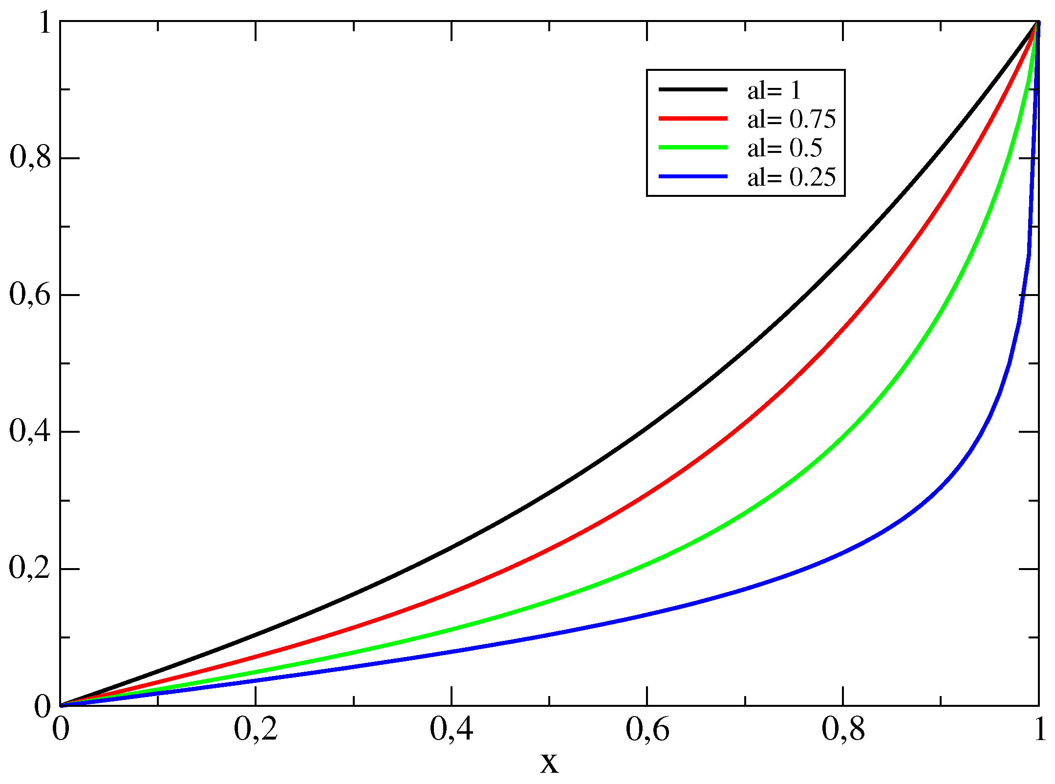
The domain $\Omega$ is discretized using $J=100$ points, the time step $\tau =0.002$ is selected for time integration. The discrete approximation of the diffusion operator $A_h$ is defined in (25). The same parameter $m=12$ of the AAA algorithm is used in all experiments. The results are presented in Figure 1.

It is clearly seen that the level of the substrate inside of a tube is decreased when the fractional power parameter is decreased and this change is most expressed at the boundary of the domain.

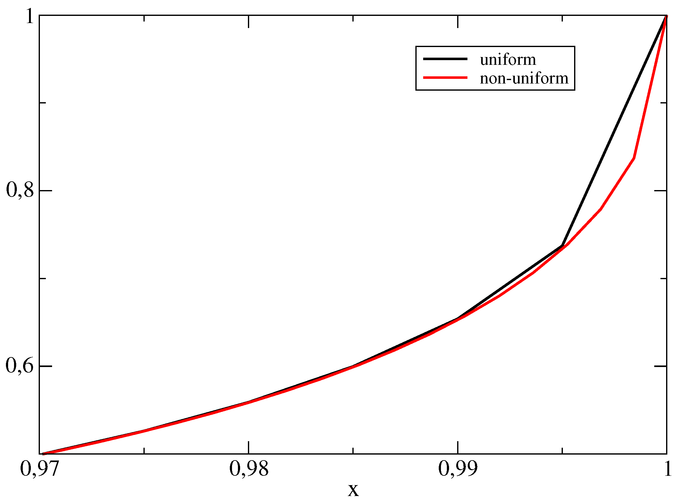
Next we demonstrate the universality of the proposed algorithms, since they can be used without any changes to solve the problem on non-uniform space meshes and for more general diffusion operators, when the diffusion coefficient is not constant. As an example we solve problem (34), when the following non-uniform graded mesh is used:

$${\omega }_h=\left\{x_j:x_j=x_{j-1}+h_{j-1/2},j=1,\dots ,J,x_0=0,x_J=1\right\},h_{j-1/2}=h{e}^{-2j/J}.$$

Then the discrete operator $A_h$ is defined as

$$\begin{array}{cc}\hfill & A_{h}U=-\frac{1}{h_j}\left(\frac{U_{j+1}-U_j}{h_{j+1/2}}-\frac{U_j-U_{j-1}}{h_{j-1/2}}\right),h_j=\frac{h_{j-1/2}+h_{j+1/2}}{2},j=1,\dots ,J-1.\hfill \end{array}$$

(35)

The eigenvalues of this operator can be bounded from above as ${\lambda }_j⩽4/\left(h_{J-1}^2\right)$, this estimate is used in the AAA algorithm to compute the rational approximation of $A_h^{-\beta }$. In Figure 2 we compare the solutions for the case of $\alpha =0.25$, $J=200$, $t=0.5$. It is clearly seen that the solution obtained using the non-uniform mesh resolves the boundary layer much better.

6.2. Allen–Cahn Equation

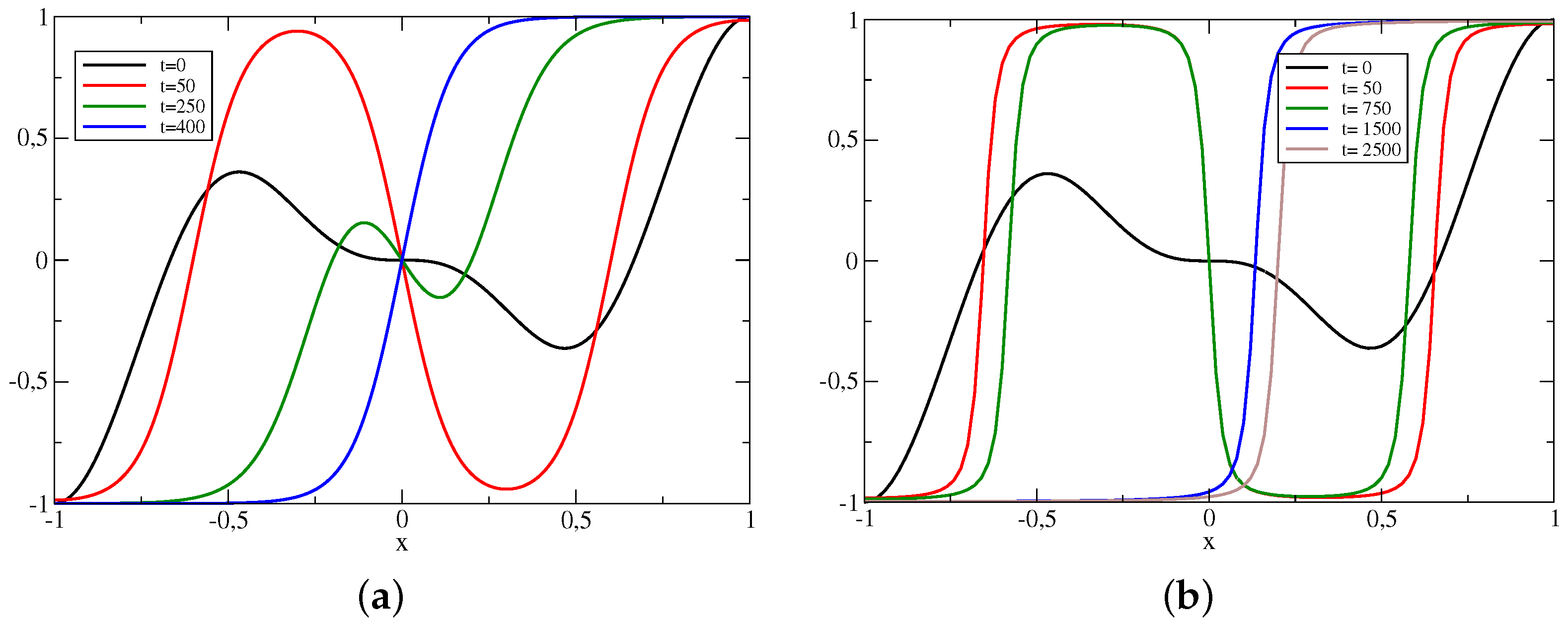
The Allen–Cahn equation is a simple nonlinear reaction-diffusion model that is used to study a formation and motion of phase boundaries. The fractional in space version of this equation is defined as [30]

$$\begin{array}{cc}\hfill & \frac{\partial u}{\partial t}=-k{\left(-\frac{{\partial }^2}{\partial x^2}\right)}^{\alpha }u+u-u^3,(x,t)\in \Omega \times (0,T],\hfill \\ \hfill & \frac{\partial u}{\partial x}(-1,t)=0,\frac{\partial u}{\partial x}(1,t)=0,t\in [0,T],\hfill \\ \hfill & u(x,0)=u_0\left(x\right),x\in [-1,1],\hfill \end{array}$$

(36)

where k is a small positive constant. It is well known, that the two steady states $u=\pm 1$ are attracting, and the third one $u=0$ is unstable. Solutions exhibit flat areas around these two stable values separated by interfaces of increasing sharpness as the control parameter k is reduced to zero.

The homogeneous Neumann boundary conditions are used in this model. A discrete approximation of these conditions is done by using the finite volume method. The accuracy of discrete boundary conditions is of the second order, i.e., the same as approximation accuracy of the differential equation. The obtained discrete operator $A_h$ is self-adjoint and positive definite.

Some effects of fractional diffusion on the metastability of the solutions has been studied in [30]. Our main aim is to test the accuracy of the general splitting scheme (29)–(32) in resolving these metastability effects. We note that the proposed discrete scheme gives at least two additional advantages—first, it can be used on non-uniform space meshes, second, even for strong nonlinear reactions only one non-local subproblem is solved at each time step. Again, we use the AAA algorithm to construct the rational approximation of fractional power elliptic operators.

As in [30] we have investigated the effect of varying fractional power parameter $\alpha$ in the metastability of solutions of the Allen–Cahn equation with parameter $k=0.01$ and initial data $u_0\left(x\right)=0.5sin\left(1.5\pi x\right)(cos\left(\pi x\right)-1)$. In all numerical experiments the number of space mesh points is $J=100$ and the time step $\tau =0.01$.

First, the case of the classical diffusion $\alpha =1$ is investigated. The results are presented in Figure 3a. At the initial stage the solution evolves to intermediate state with alternating steady states $u=\pm 1$ (see the solution at $t=50$). This state is unstable and at $t=200$ a rapid transitions begins and the solution moves to a stable state with just one interface (see the solution at $t=400$). Next we consider the case, when the fractional power parameter is decreased till $\alpha =0.65$. The results are presented in Figure 3b. It follows that the lifetime of the unstable left interface is prolonged to $t=750$, but after that a transition begins to a stable state with one interface (see solutions at $t=1500,2500$).

7. Conclusions

The given analysis show, that parabolic nonlinear reaction—nonlocal diffusion problems can be solved efficiently by the presented three discrete schemes. On the basis of obtained theoretical results and computational experiments we recommend to use the new scheme which combines the second order splitting scheme and the AAA algorithm.

One modification of the new algorithm includes an additional step when the influence of the source function is resolved at each time step by solving a nonlocal problem with a fractional power elliptic operator.

It is shown how to include nonhomogeneous boundary conditions into the discrete schemes.

Two important nonlinear reaction nonlocal diffusion models are solved. The first model describes enzyme-catalyzed reactions, the second model solves the well-known Allen–Cahn equations. The obtained results show that the nonlocal diffusion changes dynamics of nonlinear processes.

For future work it will be interesting to compare the parallel versions of the presented algorithms for solution of 3D nonstationary problems.

References

- Podlubny, I. Fractional Differential Equations, Mathematics in Science and Engineering; Academic Press: New York, NY, USA, 1999. [Google Scholar]
- Kilbas, A.A.; Srivastava, H.H.; Trujillo, J.J. Theory and Applications of Fractional Differential Equations; Elsevier Science B.V: Amsterdam, The Netherlands, 2006. [Google Scholar]
- Tarasov, V. Fractional Dynamics: Applications of Fractional Calculus to Dynamics, of Particles, Fields, and Media; Springer: Heidelberg, Germany, 2010; ISBN 10 3642140025. [Google Scholar]
- Balankin, A.S.; Espinoza Elizarraraz, B. Map of fluid flow in fractal porous medium into fractal continuum flow. Phys. Rev. E 2021, 85, 056314. [Google Scholar] [CrossRef]
- El-Nabulsi, R.A. Path integral formulation of fractionally perturbed Lagrangian oscillators on fractal. J. Stat. Phys. 2018, 172, 1617–1640. [Google Scholar] [CrossRef]
- Gomez-Aguilarb, J.F. Fractional derivatives with no-index law property: Application to chaos and statistics. Chaos Solitons Fractals 2018, 114, 516–535. [Google Scholar]
- El-Nabulsi, R.A. Fractional Dirac operators and deformed field theory on Clifford algebra. Chaos Solitons Fractals 2009, 42, 2614–2622. [Google Scholar] [CrossRef]
- El-Nabulsi, R.A.; Wu, C.G. Fractional Complexified Field Theory from Saxena-Kumbhat Fractional Integral, Fractional Derivative of Order (α,β) and Dynamical Fractional Integral Exponent. Afr. Diaspora J. Math. New Ser. 2012, 13, 45–61. [Google Scholar]
- Jumarie, G. Table of some basic fractional calculus formulae derived from a modified Riemann-Liouville derivative for non-differentiable functions. Appl. Math. Lett. 2009, 22, 378–385. [Google Scholar] [CrossRef]
- Saxton, M.J. Anomalous subdidiffusion in fluorescence photobleaching recovery: A Monte Carlo study. Biophys. J. 2001, 81, 2226–2240. [Google Scholar] [CrossRef] [Green Version]
- Baeumer, B.; Benson, D.A.; Meershaert, M.M.; Wheatcraft, S.W. Subordinated advection-dispersion equation for contaminant transport. Water Resour. Res. 2001, 37, 1543–1550. [Google Scholar] [CrossRef]
- Metzler, R.; Klafter, J. The restaurant at the end of the random walk: Recent developments in the description of anomalous transport by fractional dynamics. J. Phys. A Math. Gen. 2004, 37, R161–R208. [Google Scholar] [CrossRef]
- Sabatelli, L.; Keating, S.; Dudley, J.; Richmond, P. Waiting time distributions in financial markets. Eur. Phys. J. B 2002, 27, 273–275. [Google Scholar] [CrossRef]
- Bueno-Orovio, A.; Kay, D.; Grau, V.; Rodriguez, B.; Burrage, K. Fractional diffusion models of cardiac electrical propagation: Role of structural heterogeneity in dispersion of repolarization. J. R. Soc. Interface 2014, 11, 20140352. [Google Scholar] [CrossRef] [PubMed] [Green Version]
- Harizanov, S.; Margenov, S.; Marinov, P.; Vutov, Y. Volume constrained 2-phase segmentation method utilizing a linear system solver based on the best uniform polynomial approximation of x−1/2. J. Comput. Appl. Math. 2017, 310, 115–128. [Google Scholar] [CrossRef]
- Pozrikidis, C. The Fractional Laplacian; CRC Press: Boca Raton, FL, USA, 2016. [Google Scholar]
- Lee, H.G. A second-order operator splitting Fourier spectral method for fractional-in-space reaction–diffusion equations. J. Comput. Appl. Math. 2018, 333, 395–403. [Google Scholar] [CrossRef]
- Hofreither, C. A unified view of some numerical methods for fractional diffusion. Comput. Math. Appl. 2020, 80, 332–350. [Google Scholar] [CrossRef]
- Bonito, A.; Pasciak, J.E. Numerical approximation of fractional powers of elliptic operators. Math. Comput. 2015, 84, 2083–2110. [Google Scholar] [CrossRef] [Green Version]
- Harizanov, S.; Lazarov, R.; Margenov, S.; Marinov, P.; Vutov, Y. Optimal solvers for linear systems with fractional powers of sparse SPD matrices. Numer. Linear Algebra Appl. 2018, 25, e2167. [Google Scholar] [CrossRef]
- Nakatsukasa, Y.; Sete, O.; Trefethen, L.N. The AAA algorithm for rational approximation. SIAM J. Sci. Comput. 2018, 40, A1494–A1522. [Google Scholar] [CrossRef]
- Nochetto, R.H.; Otarola, E.; Salgado, A.J. A PDE approach to fractional diffusion in general domains: A priori error analysis. Found. Comput. Math. 2015, 15, 733–791. [Google Scholar] [CrossRef] [Green Version]
- Bonito, A.; Borthagaray, J.P.; Nochetto, R.H.; Otarola, E.; Salgado, A.J. Numerical methods for fractional diffusion. Comput. Vis. Sci. 2018, 19, 19–46. [Google Scholar] [CrossRef] [Green Version]
- Banjai, L.; Melenk, J.M.; Nochetto, R.H.; Otarola, E.; Salgado, A.J.; Schwab, C. Tensor FEM for spectral fractional diffusion. Found. Comput. Math. 2019, 19, 901–962. [Google Scholar] [CrossRef] [Green Version]
- Vabishchevich, P.N. Numerically solving an equation for fractional powers of elliptic operators. J. Comput. 2015, 282, 289–302. [Google Scholar] [CrossRef] [Green Version]
- Čiegis, R.; Vabishchevich, P.N. Two-level schemes of Cauchy problem method for solving fractional powers of elliptic operators. Comput. Math. Appl. 2020, 80, 305–315. [Google Scholar] [CrossRef]
- Čiegis, R.; Vabishchevich, P.N. High order numerical schemes for solving fractional powers of elliptic operators. J. Comput. Appl. Math. 2020, 372, 112627. [Google Scholar] [CrossRef] [Green Version]
- Tadjeran, C.; Meerschaert, M.M.; Scheffler, H.P. A second-order accurate numerical approximation for the fractional diffusion equation. J. Comput. Phys. 2006, 213, 205–213. [Google Scholar] [CrossRef]
- Zhang, H.; Jianga, X.; Zeng, F.; Karniadakis, G.E. A stabilized semi-implicit Fourier spectral method for nonlinear space-fractional reaction-diffusion equations. J. Comput. Phys. 2020, 405, 109141. [Google Scholar] [CrossRef] [Green Version]
- Bueno-Orovio, A.; Kay, D.; Burrage, K. Fourier spectral methods for fractional-in-space reaction-diffusion equations. Bit Numer. Math. 2014, 54, 937–954. [Google Scholar] [CrossRef]
- Alzahrani, S.S.; Khaliq, A.Q.M. Fourier spectral exponential time differencing methods for multi-dimensional space-fractional reaction–diffusion equations. J. Comput. Appl. Math. 2019, 361, 157–175. [Google Scholar] [CrossRef]
- Banjai, L.; Otarola, E. A PDE approach to fractional diffusion: A space–fractional wave equation. Numer. Math. 2019, 143, 177–222. [Google Scholar] [CrossRef] [Green Version]
- Melenk, J.M.; Rieder, A. hp-FEM for the fractional heat equation. Ima J. Numer. Anal. 2021, 41, 412–454. [Google Scholar] [CrossRef]
- Yang, Q.; Turner, I.; Liu, F.; Ilic, M. Novel numerical methods for solving the time-space fractional diffusion equations in two dimensions. SIAM J. Sci. Comput. 2011, 33, 1159–1180. [Google Scholar] [CrossRef] [Green Version]
- Yang, Q.; Turner, I.; Moroney, T.; Liu, F. A finite volume scheme with preconditioned Lanczos method for two-dimensional space-fractional reaction-diffusion equations. Appl. Math. Model. 2014, 38, 3755–3762. [Google Scholar] [CrossRef] [Green Version]
- Li, Q.; Song, F. Splitting spectral element method for fractional reaction-diffusion equations. J. Algorithms Comput. Technol. 2020, 14, 1–10. [Google Scholar] [CrossRef]
- Vabishchevich, P.N. Splitting schemes for non-stationary problems with a rational approximation for fractional powers of the operator. Appl. Numer. Math. 2021, 165, 414–430. [Google Scholar] [CrossRef]
- Čiegis, R.; Starikovičius, V.; Margenov, S.; Kriauzienė, R. Parallel solvers for fractional power diffusion problems. Concurr. Comput. Pract. Exp. 2017, 29, e4216. [Google Scholar] [CrossRef]
- Čiegis, R.; Starikovičius, V.; Margenov, S.; Kriauzienė, R. Scalability analysis of different parallel solvers for 3D fractional power diffusion problems. Concurr. Comput. Pract. Exper. 2019, 31, e5163. [Google Scholar] [CrossRef]
- Burch, N. Classical, nonlocal and fractional diffusion equations on bounded domains. Int. J. Multiscale Com. 2011, 9, 661–674. [Google Scholar] [CrossRef] [Green Version]
- Yuste, S.B. Weighted average finite difference methods forfractional diffusion equations. J. Comput. Phys. 2006, 216, 264–274. [Google Scholar] [CrossRef] [Green Version]
- Nochetto, R.H.; Otarola, E.; Salgado, A.J. A PDE approach to space-time fractional parabolic problems. Siam J. Numer. Anal. 2016, 54, 848–873. [Google Scholar] [CrossRef] [Green Version]
- Ilic, M.; Liu, F.; Turner, I.W.; Anh, V. Numerical approximation of a fractional-in-space diffusion equation–II-with nonhomogeneous boundary conditions. Fract. Calc. Appl. Anal. 2006, 9, 333–349. [Google Scholar]
- Baronas, R.; Kulys, J.; Petkevičius, L. Modelling the enzyme catalysed substrate conversion in a microbioreactor acting in continuous flow mode. Nonlinear Anal. Model. Control 2018, 23, 437–456. [Google Scholar] [CrossRef] [Green Version]
- Garcia-Viloca, K.; Gao, J.; Karplus, M.; Truhlar, D. How enzymes work: Analysis by modern rate theory and computer simulations. Science 2004, 303, 186–195. [Google Scholar] [CrossRef] [PubMed]
Figure 1.
Distribution of the substrate at for different fractional power parameters .
Figure 2.
Distribution of the substrate at for the fractional power parameter in the cases of uniform and non-uniform meshes.
Figure 3.
Dynamics of the solutions of the Allen–Cahn equation for varying the fractional power parameter: (a) the classical diffusion process , (b) the fractional diffusion process .