
Abstract
Understanding how the brain functions is one of the grand challenges in modern scientific research. Similar to a computer, a functional brain is composed of hardware and software. The major bottleneck lies in the difficulty to directly observe the brain 'software', i.e. the rule and operating information used by the brain that might emerge from pan-neuron/synapse connectome. A recognized strategy for probing the functional connectome is to perform volumetric imaging in brains with high spatiotemporal resolution and deep brain penetration. Among various imaging technologies, optical imaging offers appealing combinations including spatial resolution of sub-micrometer to nanometer, temporal resolution of second to millisecond, penetration depth of millimeter or deeper, and molecular contrast based on the abundant choices of fluorescent indicators. Thus, it is ideal for enabling three-dimensional functional brain mapping of small animal models. In this review, we focus on recent technological advances in optical volumetric imaging, with an emphasis on the tools and methods for enhancing imaging speed, depth, and resolution. The review could serve as a quantitative reference for physicists and biologists to choose the techniques better suited for specific applications, as well as to stimulate novel technical developments to advance brain research.
Export citation and abstract BibTeX RIS

Original content from this work may be used under the terms of the Creative Commons Attribution 4.0 license. Any further distribution of this work must maintain attribution to the author(s) and the title of the work, journal citation and DOI.
1. Introduction
One of the greatest scientific challenges in the 21st century is to understand what consciousness is and how the brain functions. In the 125-anniversary special issue of the journal Science (1 July 2005), 125 significant scientific questions were identified, wherein the top questions are: 'What Is the biological basis of consciousness?' and 'how are memories stored and retrieved?' [1]. Nevertheless, after more than a decade, these questions are still unresolved. In fact, since the era of Golgi and Cajal, the pursuit to understand the brain, which is composed of thousands to millions of densely packed neurons, through mapping interconnections among neurons (i.e. connectomes) has lasted for more than a century [2, 3]. Anatomical analyses using state-of-the-art electron microscopy (EM) have impressively revealed the structural connections among neurons across a whole Drosophila brain [4]. Note that a Drosophila brain is composed of 105 neurons, tightly packed in a volume of less than 1 mm3, and it already takes at least a month to finish EM mapping of the brain. Considering that a mouse brain has 108 neurons in ∼1 cm3 volume, and a human brain has 1011 neurons in ∼1000 cm3 volume, it will take decades and millennia to map a mouse and a human brain respectively with EM.
Nevertheless, even if these high-resolution connectomes are achieved, say through large-scale parallel imaging, brain functions may still remain mysterious since such anatomical studies only map the 'hardware' connectome. Considering the current understanding of how a computer works, it is far from enough to merely look at the hardware connections, it is necessary to also understand the underlying software. According to the Oxford dictionary, software is defined as 'the programs and other operating information used by a computer'. In the context of brain operation, software may be defined as 'the rules and other operating information used by a brain', that should be an emergent property from the underlying collective neural activities. In our viewpoint, the main bottleneck for understanding a brain now is that no existing techniques or imaging methods are capable of directly unraveling the 'software' or information content of a brain, not to mention further understanding consciousness and memory.
Although the software may not be easily visible, one potential direction is to map the functional activities in the neuronal 'hardware', which allows us to peek into the 'software' through observing the information flow, and gradually reconstruct the software. Conventionally, since information flow in neurons rely on ion-induced voltage transduction, electroencephalography (EEG) or electrophysiology methods are used to probe the functional response of the brain. The main advantage of electric methods is their outstanding temporal resolution and high signal-to-noise ratio. Through a non-invasive patch, EEG enables high-speed (millisecond) volumetric imaging of a whole human brain, but its spatial resolution is typically centimeters, far below single cell level (∼10 µm). On the other hand, electrophysiology samples action potentials down to single neuron or even single axon scale, but to avoid interfering with brain function, the number of invasive microelectrodes has to be limited.
For non-invasive imaging of the brain, medical modalities such as magnetic resonance imaging (MRI), positron-emission tomography and ultrasound, provide three-dimensional (3D) imaging across a whole human brain but do not have adequate spatial/temporal resolution to resolve individual neurons and their ionic/electric dynamics. More importantly, the contrast sources of these medical imaging systems do not directly reflect ion or voltage signals in neurons. For example, functional MRI measures the oxygenation level of hemoglobin, as an indirect indicator of brain region functions.
High-resolution imaging modalities such as atomic force microscopy or EM offer excellent spatial resolution down to nanometer regime, though these are limited to only surface observations. For brain tissue imaging, it is necessary to microtome an intact brain into many thin slices, which not only is challenging in maintaining the sophisticated neural connections and in time consumption, but prohibits in vivo observations to correlate fine spatial details to functional information encoded in these connections (not to mention that EM requires vacuum environment). Note that optical microscopy, when combined with sophisticated genetic tools, does allow examination of functional connectivity after sacrificing the experimental animal, i.e. ex vivo observation [5].
Here we focus on optical imaging methods that potentially enable the study of multiscale functional connectome with high spatiotemporal resolution, in a whole small animal brain, in vivo or ex vivo. Compared to electrophysiology, the signal-to-noise ratio of optical methods is inferior, but the latter enables simultaneous observation of a large number of neurons, whose 'emerging' physiological behaviors cannot be found by studying only a few neurons. Compared to medical imaging modalities, optical imaging has less penetration depth, but the resolution is at least sub-cellular, potentially down to synapse level with the aid of super-resolution technologies. Compared to EM, even though the resolution of optical imaging is lower, the capability of noninvasive observation allows optical methods to capture action potential firings with a single neuron, which is currently not possible with EM. Therefore, optical imaging would be the ideal tool to study brain functional connectomes in a small model animal [6–9].
When we consider optical imaging technology (or any imaging methods), there are at least four fundamental parameters to address, namely contrast, spatial resolution, temporal resolution and imaging depth. There are various developments in terms of optical contrasts that enable visualization of functional interactions among neurons. The readers are encouraged to read recent review articles for contrast development, such as genetically encoded indicators or hybrid fluorescent probes [10–14]. With the aid of fluorescent labeling, it is possible to monitor neural responses with sub-second temporal resolution in vivo [15, 16]. In this review, we will put more emphasis on technical development of optical systems. In particular, to observe the emergent property from functional connectome, not only is high-speed volumetric imaging highly desirable, but also techniques that can increase penetration depth to cover a large brain volume, as well as methods to improve spatial resolution under volumetric imaging. Please note that non-fluorescent imaging techniques like optical coherence tomography are not included in this review. In the following, we will address recent technological advances on three main factors of volumetric imaging: imaging speed (section 2, sub-second to millisecond), penetration depth (section 3, millimeter and beyond), and spatial resolution enhancement (section 4, micrometer to nanometer).
2. Review of high-speed volumetric imaging technologies
Recording and thus understanding the swift and convoluted interactions between neurons is an overarching goal of neuroscience. To achieve the goal using optics, it requires observation of neural activities over large volumes with sub-second to millisecond temporal resolution, i.e. high-speed volumetric imaging. It is generally accepted that optical sectioning, a depth-resolved ability to distinguish different layers, is necessary for volumetric imaging in biological tissues. Confocal microscopy (CM), which was invented half a century ago, achieves optical sectioning with single-photon excitation via laser scanning, a confocal pinhole, and a point detector. To enhance penetration depth and emission photon collection efficiency, multiphoton microscopy, which was demonstrated in 1990 [17], achieves intrinsic optical sectioning through multiphoton excitation via laser scanning and a point detector. Nevertheless, raster scanning plus point detection is generally slow, since adequate accumulation time is required for each pixel/voxel. A different approach is to utilize wide-field detection via a camera, and combine with novel strategies for optical sectioning, such as light-sheet microscopy (LSM) (section 2.1.2).
Overall speaking, high-speed volumetric imaging is achieved through either excitation schemes (single-photon or multiphoton) or detection design (camera or point detector). Single-photon excitation is better in fluorescence yield, and multiphoton excitation typically exhibits better penetration depth with intrinsic optical sectioning. Camera-based (or wide-field detection) techniques provide outstanding digital resolution (i.e. number of pixels/voxels), but suffer from tissue scattering/aberration induced crosstalk, which means signals from different locations in the specimen contaminate one another, so the penetration depth is limited. On the other hand, a point detector collects all scattering photons into one pixel/voxel, thus becoming free from the crosstalk issue. To achieve high-speed brain imaging in large volumes of interest, optical sectioning and the solution of cross-talk are both necessary. Figure 1 summarizes the categories of different excitation and detection designs (1PE Camera, 2PE Camera, 1PE PD, and 2PE PD). Note that different spatial sampling techniques, as discussed in [7], are all covered in the figure. In the following, we will review recent progress of high-speed volumetric imaging that provides optical sectioning with camera-based detection (section 2.1), and then point-detector-based techniques that deal with cross-talk will be discussed (section 2.2).

Figure 1. Summary of high-speed volumetric imaging techniques. Schematic illustration of the principles of (a1)–(a4) camera-based techniques with (mostly) single photon excitation (1PE): (a1) wide-field microscopy (WF), (a2) spinning disk confocal microscopy (SDCM), (a3) light-sheet microscopy (LSM), and (a4) light-field microscopy (LFM). (b1), (b2) Camera-based techniques with two-photon excitation (2PE): (b1) temporal focusing microscopy (TF), (b2) spatially multiplexed microscopy (SM). (c) Point-detector (PD) based technique with mostly 1PE: frequency multiplexed system (FM). (d1)–(d8) PD based techniques with (mostly) 2PE: (d1) spatially multiplexed system, (d2) spatiotemporally multiplexed system (STM), (d3) piezoelectric actuator, (d4) remote focusing (RF), (d5) electrically tunable lens (ETL), (d6) acousto-optical deflector (AOD), (d7) tunable acoustic gradient-index (TAG) lens, (d8) Bessel beam, (e) Data throughput versus penetration depth of high-speed techniques (see table 1 for details as well as the individual sample types). LS: light-sheet, G: grating, PMT: photomultiplier tube, MAPMT: multi-anode PMT, AOD: acousto-optical deflector, AL: axicon lens.
Download figure:
Standard image High-resolution imageTable 1. Comparison of various high-speed volumetric imaging techniques modalities.
| Category | Volume/frame per second | Volume size (µm3) | Throughput (voxels s−1) | Sample type | Reference |
|---|---|---|---|---|---|
| Camera + (Mostly) 1PE | |||||
| SDCM | ∼60 fps a | ∼200 × 200 × 100 | ∼4 × 10⁸ | Mouse brain | [21] |
| 2pSDCM | ∼8 fps a | ∼200 × 200 × 500 | ∼1 × 10⁶ | Mouse brain | [23] |
| LSM + ETL | 30 | ∼200 × 150 × 100 | ∼1 × 10⁸ | Zebrafish | [30] |
| LSM + TAG | 200 | ∼150 × 150 × 100 | ∼5 × 10⁸ | Paramecium | [31] |
| SCAPE | 25 | ∼400 × 300 × 40 | ∼8 × 10⁸ | Mouse brain/ fly larvae | [37], maximal depth ∼ 100 µm |
| CLAM | ∼10 | ∼230 × 70 × 70 | ∼4 × 10⁶ | Cleared mouse tissue | [41], maximal depth ∼ 100 µm |
| 2pLSM | ∼70 fps a | ∼160 × 160 × 100 | ∼4 × 10⁷ | Zebrafish/Fly | [45–48] |
| Miniaturized LFM | ∼20 | 700 × 600 × 360 | ∼3 × 10⁹ | Mouse brain | [54] |
| Dual view LFM | ∼150 | 300 × 300 × 300 | ∼1 × 10¹⁰ | Medaka | [55] |
| Camera + 2PE | |||||
| TF | 5 | 500 × 500 × 500 | ∼3 × 10⁶ | Mouse brain | [65] |
| Mul. TF | 17 | 700 × 700 × 600 | ∼2 × 10⁷ | Mouse brain | [66] |
| SLM + MMM | 10 | 600 × 600 × 200 | ∼1 × 10³ | Mouse brain | [74], sparse |
| SLM + MMM + GL | 100 | 200 × 200 × 50 | ∼1 × 10⁴ | Cultured neurons | [75], sparse |
| PD + (Mostly) 1PE | |||||
| Freq. mul. | 104 | 70 × 80 × 90 | ∼7 × 10⁸ | Microalgae | [82] |
| PD + (mostly) 2PE | |||||
| Spa. mul. | 0.3–1 fps a | 360 × 360 | ∼3 × 10⁴ | Mouse brain | [89], maximal depth ∼ 200 µm |
| Spa. tem. mul. | 3000 fps a | 50 × 250 | ∼3 × 10⁸ | Mouse brain | [95], maximal depth ∼ 350 µm |
| Piezoelectric | 10 | 250 × 250 × 500 | ∼1 × 10⁵ | Mouse brain | [102] |
| Remote focusing | 6 | ∼300 × 150 × 300 | ∼7 × 10⁶ | Zebrafish brain | [135], maximal depth ∼ 500 µm |
| Liquid lens | 10 | 145 × 75 × 500 | ∼5.1 × 10⁵ | Mouse brain | [111], only 2–3 planes in z |
| 2pAOD | 82 | 500 × 500 × 650 | ∼2.4 × 10⁶ | Mouse brain | [121] |
| 2pAOD | 40 fps a | 250 × 250 × 250 | ∼1 × 10⁷ | Mouse brain | [122], maximal depth ∼ 500 µm |
| 2pTAG | 14 | 400 × 300 × 500 | ∼4 × 10⁷ | Mouse brain | [125, 126] |
| 2pBessel | 3.2 | ∼200 × 450 × 600 | ∼1.6 × 10⁷ | Mouse brain | [134] |
| 3pBessel | 5 | 500 × 500 × 300 | ∼3.3 × 10⁵ | Mouse brain | [133], maximal depth ∼700 µm |
a fps: 2D frame per second. Axial step is controlled by a translational stage, so throughput is calculated by a specific volume demonstrated in the paper.
2.1. Camera-based techniques
When using cameras (or our eyes) for detection, the most straightforward excitation geometry is single-photon wide-field illumination, which was used by Golgi and Cajal when they found branch-like cells in brains. As shown in figure 1(a1), white light illuminates the whole tissue volume along the light path, and transmission or fluorescence signals from the entire sample are captured simultaneously by eyes or cameras. The spatial resolution reaches hundreds of nanometers, which is sufficient to recognize a single neuron or even fiber networks across complex neuron connections. However, wide-field microscopy lacks optical sectioning, and in scattering tissues, suffers from crosstalk, so the imaging depth is typically limited to much below 100 µm in the mouse brain [18]. Below we will discuss different excitation schemes, including single-photon confocal excitation, light-sheet excitation, and multi-photon excitation, that combine with camera-based detection to provide optical sectioning for brain imaging. In addition, a special detection scheme that combines lens array with (mostly) single photon excitation to enable multiple layer imaging simultaneously, i.e. light-field microscopy (LFM), will also be addressed.
2.1.1. (Mostly 1PE) Spinning disk CM.
Stemming from the concept of CM, spinning disk CM (SDCM) [19] integrates a rotating microlens array to create hundreds of foci simultaneously scanning at the focal plane, a co-rotating pinhole array to achieve optical sectioning, and a high-speed camera to capture fluorescence emissions. Figure 1(a2) is the schematic layout of a SDCM. It provides up to 1000 frame s−1 imaging speed [20], much higher than CM, as well as usually better SNR because the camera provides higher quantum efficiency (∼80%) than point detectors such as photomultiplier tubes (∼30%). For brain tissue imaging, SDCM combined with an 8 K ultra-high-definition CMOS camera achieves mouse brain imaging with 60 frames s−1 (5310 × 4320 pixels), which equivalently has about a throughput of 382 megapixel per second [21]. One important advantage of SDCM is reduced photobleaching and photodamage because of the high-speed movement of focal spots, thus more suitable for in vivo imaging [22].
However, due to the single photon excitation of SDCM, the penetration depth is limited to less than 100 μm in the mouse brain. To further increase the imaging depth, two photon SDCM (2pSDCM) has been demonstrated to enhance the penetration depth up to 500 μm deep in the mouse brain [23]. 2pSDCM also eliminated the issue of out-of-focus bleaching in SDCM. For more discussion on multiplexed multiphoton microscopy, i.e. converting a single focus to multiple foci, please refer to sections 2.1.5 and 2.2.1.
2.1.2. (Mostly 1PE) LSM.
Another strategy to achieve optical sectioning and refrain from out-of-focus bleaching is to avoid epi-detection, but to arrange excitation and detection in a perpendicular format (figure 1(a3)), thus eliminating out-of-focus excitation. This concept was demonstrated with not only scattering observation [24] but also fluorescence microscopy, known as selective plane illumination microscopy [25, 26], or LSM [27, 28]. Recently, there is a surge of applying LSM toward neuroscience, enabling high-speed acquisition, such as 10 volumes s−1 observation in a living mouse brain. It is not within the scope of this review to cover the complete literature review of LSM, instead we refer interested readers to recent reviews [27, 28]. One major advantage of LSM is its side illumination that prevents out-of-focus photobleaching under single-photon excitation [27, 29]. By combining with an electrically or acoustically tunable lens, the volumetric imaging rate of LSM exceeds 100 volume s−1 [30, 31].
With two perpendicular objectives, one main limitation in conventional LSM is the trade-off between field-of-view (FOV) and axial resolution due to the constraint of Gaussian beam focusing. This is relieved by adopting non-diffracting Bessel beam illumination [32]. Bessel beam also helps to improve the excitation beam penetration depth of LSM [33]. Furthermore, by arranging multiple Bessel beams into an array, in 2014 Chen et al demonstrated lattice light sheet microscopy (LLSM) [34], which enabled significant reduction of photobleaching/phototoxicity, as well as enhanced spatial resolution by two-fold. Combining with expansion microscopy [35] (see section 4.3), this powerful technique can image millions of synapses in an ex vivo entire Drosophila brain within a few days, much faster than EM.
To facilitate in vivo volumetric observation in a living animal brain, an innovative idea of swept, confocally-aligned planar excitation (SCAPE) microscopy was developed recently [36]. It combines the concept of light sheet and confocal imaging, and uses only a single objective for both illumination and detection, making sample positioning and alignment much simpler than conventional light-sheet imaging. The latest version of SCAPE can achieve impressively 300 volumes s−1 imaging speed in brain tissues, i.e. over 1.2 GHz voxel rates [37].
Another strategy for enhancing the LSM speed is parallelized multi-light-sheet generation (from a few to tens of light sheets), which can be realized by a number of methods, including interferometry, wavefront engineering, beam splitting, and more recently the concept of 'infinity mirror' [38–42]. An important advantage of such parallelization is to maximize the spatial duty cycle, and thus photon budget [41]—a critical attribute for ensuring the viability of imaged samples.
Because of sample absorption and scattering, striping artifacts may appear in LSM and affect the image quality, and several approaches have been proposed to overcome those artifacts [29, 43, 44]. Moreover, the thickness of the light sheet grows when imaging deep in the tissue, not only deteriorating the axial resolution but also reducing the signal strength on the far side of illumination. The scattering effect on the excitation beam can be relieved via long wavelength excitation (see section 3.3), such as two-photon LSM (2pLSM) [45–49] or even three-photon LSM [50]. However, in the wide-field detection arm, tissue scattering still induces crosstalk on the camera, thus blurring the images. Furthermore, due to the quadratic two-photon excitation, the effective FOV of 2pLSM [45] is smaller than that in single-photon LSM [26]. A more practical strategy for deep-tissue LSM is to adopt near-infrared excitation and emission with quantum dots, that allows 750 µm imaging depth in a living mouse brain [51].
2.1.3. (Mostly 1PE) LFM.
Instead of pursuing optical sectioning in orthographic or perpendicular schemes, volumetric imaging can also be achieved via parallax effects, which is fundamental to our stereo vision. First demonstrated in 2006 by M Levoy, LFM utilizes a microlens array inserted at the intermediate image plane of a microscope, simultaneously recording the lateral and angular information of light, i.e. light field as shown in figure 1(a4), to reconstruct a 3D image, at the cost of spatial resolution [52]. The potential of LFM on high-speed volumetric imaging was soon realized by the neuroscience community, demonstrating Ca+2 dynamics at 10–20 Hz in the brain of larval zebrafish [53] and the hippocampus of freely moving mice [54]. More recently, by innovatively applying selective-volume illumination and collecting orthogonal light fields, LFM achieves impressively 200 Hz volume rate with 2 μm isotropic spatial resolution [55]. The spatial resolution may be further enhanced by 1.4-fold via speckle-based structured illumination [56].
Since LFM relies on modification in the detection path, it can be combined with other wide-field illumination methods, such as light sheet microscopy [57], that allows selective plane excitation and enhanced spatial resolution. Alternatively, combining LFM with confocal detection can maintain high resolution at depths of hundreds of micrometers [58]. Very recently, wide-field two-photon excitation based on temporal focusing was combined with LFM, further enhancing the penetration depth [59]. Below we briefly introduce the concept of temporal focusing, which allows wide-field epi-detection together with multiphoton excitation.
2.1.4. (2PE) Temporal focusing.
First demonstrated in 2005, temporal focusing, as its name suggests, makes an ultrashort pulse temporally compressed (focused) at the focal plane, and thus maximizes the multiphoton contrast at the focus, enabling optical sectioning under wide-field excitation scheme [60–62]. The simplified layout of temporal focusing is shown in figure 1(b1). An ultrashort pulse, which is spectrally broad, is stretched in time and dispersed in space by a diffraction grating that is conjugate to the objective focal plane. At the focal plane, the dispersed spectrum is recombined and the short pulse with high peak intensity is recovered to permit multiphoton excitation.
With the capability of wide-field illumination and detection, temporal focusing facilitates high-speed functional imaging in the brain, such as in brain slices [63], Caenorhabditis elegans [64] and mouse, achieving 160 Hz frame rate and 3–6 Hz volume rate in a mouse cortical column (0.5 mm × 0.5 mm × 0.5 mm) [65]. Combined with beam multiplexing and remote focusing (RF), temporal focusing enables ∼0.7 mm × ∼ 0.7 mm × ∼0.6 mm volume imaging at nearly 17 Hz [66].
A trade-off in temporal focusing is FOV and power limitation [67]. Since the laser beam is spatially spread across an area, the excitation photon density decreases. To achieve large volume imaging, high energy lasers are necessary, and may lead to photodamage [8]. In addition, due to its wide-field detection nature, cross-talk on the camera plane still limits the penetration depth of temporal focusing to below 500 µm [68]. Currently temporal focusing is used primarily for patterned stimulation, instead of imaging [67]. To reduce the concern of phototoxicity and signal cross-talk, a potential strategy is simultaneous but sparse two-photon excitation spots via spatial multiplexing, which is mentioned in the following section.
2.1.5. (2PE) Spatially multiplexed two-photon microscopy.
Spatially multiplexed multiphoton microscopy, or multifocal multiphoton microscopy (MMM), was proposed more than two decades ago [69, 70]. The early versions are based on lens arrays and camera detection (similar to SDCM in section 2.1.1), which already enable video-rate imaging. For PMT-based MMM, please see section 2.2.1. However, the lens array typically suffers from significant transmission loss. It is well known in holography that a phase mask can generate multiple focal spots at different 3D locations with high efficiency [71]. A more convenient and precise way for brain imaging is to use a spatial light modulator (SLM), i.e. a tunable phase mask, to create multiple foci that selectively target individual neurons, and the 3D emitted fluorescence photons are projected back to a 2D camera, as shown in figure 1(b2). Such spatially multiplexed two-photon microscopy, first demonstrated in 2008 [72], does not require any laser scanning but allows >10 Hz sampling among tens of targeted neurons [73].
Over the past decade, various advances of holographic MMM have been demonstrated. For example, temporal multiplexing via galvo mirrors was integrated into SLM-based MMM to enable observation of ∼100 neurons in the mouse cortex spanning 600 µm × 600 µm × 200 µm at 10 Hz in vivo [74]. The volumetric detection can be optimized through introducing a Gaussian–Laguerre (GL) phase plate before the camera, thus increasing the imaging depth of field (DOF) to match the 3D multiplexed excitation foci [75]. Furthermore, combined with temporal focusing, multiplexed foci allow volumetric two-photon photoactivation or photoconversion of fluorescent proteins in a volume size of 106 µm3 [76, 77].
The idea of SLM-based MMM is to target only neurons of interest in a volume with pre-requisite knowledge of neuron distribution, thus saving a lot of time from full-volume sampling. Nevertheless, this idea brings along a weakness that the system is susceptible to movement of living animals. Moreover, one potential limitation of the SLM-based technique is the direct 3D volume to 2D camera projection that is not able to distinguish neurons located at the same lateral positions but at different depths. Instead of using camera detection, the concept of spatiotemporally multiplexing can be combined with a point detector, that enables multiplane imaging with aberration correction (see section 2.2.1). Next, we review recent progress of high-speed volumetric imaging based on highly sensitive point detector(s), such as PMT or avalanche detector(s).
2.2. Point-detector-based techniques
In section 2.1, cameras are combined with wide-field or multi-point excitation schemes to detect excited fluorescence signals. However, wide-field detection is susceptible to signal crosstalk, which limits the imaging depth in scattering tissues. In contrast, methods based on point detectors are less affected by scattering, but with the price of reduced imaging speed due to its scanning nature. It is important to highlight that the data throughput of a single high-speed point detector, such as a PMT or silicon photomultiplier, may achieve ∼1 GHz [78], which is comparable to the total data throughput of the millions of pixels on a camera. Therefore, when combined with beam multiplexing or high-speed scanning, PMT-based methods have the potential to provide high-speed volumetric imaging in tissues. Here we introduce several methods that aim to increase 2D/3D imaging speed by innovative frequency/spatiotemporal multiplexing of excitation beams (section 2.2.1), as well as by high-speed axial scanning techniques (section 2.2.2).
2.2.1. Spatiotemporal multiplexing.
Following the discussion in section 2.1.5, multiplexing means to transform a single beam to multiple beams, thus proportionally enhancing the imaging speed. A classic example is SDCM that we mentioned in section 2.1.1, but it is based on camera detection. Below we address point-detector based multiplexing methods that provide high volumetric acquisition with single-photon or multi-photon excitations.
2.2.1.1. (Mostly 1PE) Frequency multiplexed system.
In order to avoid the detrimental crosstalk effect of camera-based multiplexing methods, one strategy is to add frequency modulation onto each beam, and collect the emission with a single photodetector, whose bandwidth is large enough for multiple beam demodulation [79–81], as shown in figure 1(c). The state-of-the-art 1PE volumetric imaging via frequency multiplex and a single photodetector has reached impressively 104 volume s−1 based on 1PE [82]. Similar idea, but with multi-channel detectors, has been applied to significantly enhance imaging speed of multiphoton fluorescence lifetime imaging in the mouse brain [83] and coherent Raman microscopy [84]. In the following, we will concentrate on multiphoton based techniques that enhance both imaging speed and depth (see section 3.3) for tissue observations.
2.2.1.2. (2PE) Spatially multiplexed system.
Typical multiphoton imaging is achieved through laser scanning a single tightly focused spot of high-intensity pulses, thus limiting its imaging speed. After combining with spatial multiplexing, as shown in figure 1(d1), the speed increases proportionally with the number of foci. In this section, we address PMT-based MMM, where a single PMT or a multi-channel PMT could be used.
When utilizing a single PMT in MMM, the same strategy of frequency multiplexing was applied via creating multiple beams by a SLM and encoding them at different frequencies by a digital mirror device, thus achieving a scanless microscope that traces voltage/calcium dynamics in cells, brain slices, and living mouse brains, with millisecond temporal resolution [85]. Another method is to combine SLM-generated multiplexed foci in different axial locations and lateral scan with galvo mirrors, to achieve simultaneous multi-plane imaging. With the prior knowledge of sparsely distributed neurons, plus an extensive computation algorithm, three multiplane images across 300 × 300 × 300 µm3 is resolved at 10 frames s−1 [86].
Probably the most straightforward idea to realize PMT-based MMM is to adopt a multi-anode PMT (MAPMT) to match the multiplexed foci. It was demonstrated in 2007, with a scanning 8 × 8 foci and corresponding 8 × 8 MAPMT [87]. However, the demonstrated frame rate is relatively low, only around 1 frame s−1, due to the low transmission of their microlens array. By using a diffractive optical element, which has a much better transmission, to generate 32 × 1 multiplexed beams, and combine with a 32 × 1 MAPMT, we have achieved unprecedented two-photon imaging at 500 volumes per second, covering 200 × 200 × 200 µm3 [88]. Because of the multiple detectors, these systems may suffer from crosstalk issues, similar to camera detection. Interestingly, with the aid of image deconvolution and photon reassignment, the MAPMT-based MMM has improved depth performance in brain tissues over camera-based MMM [87, 89].
2.2.1.3. (2PE) Spatiotemporally multiplexed system.
Since two-photon excitation requires high peak intensity, ultrashort pulse lasers (∼100 fs) are typically adopted. In light of this, a possible way to prevent the crosstalk problem is to use a spatiotemporal multiplex, i.e. introducing time delay among multiple excitation beams [90], as shown schematically in figure 1(d2). With a high-speed photodetector such as PMT, a single-channel detector is adequate to collect the emitted signals and separate them in time sequence to avoid crosstalk.
To introduce the time delay, there are a few methods. The first one relies on multiple reflection/transmission of beam splitters to create tens of beams with equal intensities [91–93]. The second one integrates a reverberation loop to create multiple foci with power increasing along axial direction, thus compensating tissue scattering loss to achieve comparable fluorescence yield in each focal plane [94]. The third one adopts a pair of nearly parallel plane mirrors with a minute angular misalignment [95]. When the incident pulsed beam enters the mirror pair with different angles via a converging lens, multiple beams with different time delays are generated. The concept resembles 'infinity mirror' which generates multiple virtual source 'images' of the pulsed focused laser spot. The latter has achieved 2D imaging of in vivo neuronal activity at impressively 3000 frames s−1. We envision that the technique is readily extended into high-speed volumetric imaging by adopting axial scan methods that we are going to introduce below.
2.2.2. (2PE) High-speed axial scanning.
By reducing scattering with long wavelength excitation, 2PE provides ∼mm penetration depth, together with intrinsic optical sectioning and sub-micrometer spatial resolution. Conventionally, 2PE microscopy is based on raster scanning in the lateral direction, and sample/objective translational scanning in the axial direction. High-speed lateral scanning, via resonant mirrors or polygon mirrors, has been well documented in the early years. In this section, we review strategies to enhance volumetric imaging speed of multiphoton imaging by high-speed scanning in the axial direction, including piezoelectric actuator, RF, electrically tunable lens (ETL), inertia-free scanning, and Bessel beam.
2.2.2.1. Piezoelectric actuator.
A straightforward idea to increase axial translational scanning speed is to adopt a resonant moving stage, such as a piezoelectric actuator that allows high-speed axial movement of an objective [96], as shown in figure 1(d3). With a piezoelectric actuator, 2PE calcium imaging can reach ∼10 volume s−1 full sampling [97–99], or 700 Hz imaging speed along a 3D trajectory [100], both within ∼20 µm depth. To enhance the axial range, 3D spiral scan by synchronizing galvo scanners and a piezoelectric actuator allows 10 Hz volume rate with 200 µm depth coverage [101]. However, it is based on partial sampling, which requires sample stability, challenging for in vivo experiments. To accomplish higher volume rate across a large volume, axial scanning techniques with less inertia are desirable.
2.2.2.2. RF.
RF usually adopts a conjugate objective and a light-weight, fast-scanning mirror (figure 1(d4)) to achieve high-speed scanning at the focal plane of the imaging objective [102]. The low-inertia mirror can move axially as fast as 2.7 kHz, much faster than piezoelectric scanning [103]. An important benefit of RF is free from spherical aberration when moving focus axially. Furthermore, moving the objective that is in contact with an immersion media may introduce waves, and RF solved this issue completely. By tilting the remote scanning mirror, oblique plane imaging that fit specific neuronal directions was demonstrated [104, 105]. Combined with beam multiplexing, RF achieves 17 Hz imaging in a volume of 1.2 mm3 in an awake mouse brain, adequate to discern calcium signal dynamics [66]. Up to 100 Hz volumetric imaging rate is demonstrated by RF with a deformable mirror (DM) [106].
2.2.2.3. ETL.
ETL (ETL, figure 1(d5)) is a high-speed tunable lens that possesses less inertia than piezoelectric stages and RF mirrors. There are various mechanisms to realize the electric tunability, including electrowetting, liquid crystal, or polymer membrane [107]. For example, through the electrowetting process, an ETL can be tuned by an external electric field, at ∼100 Hz speed [108]; similarly, with a flexible membrane, an ETL can switch its focus in 15 ms [109]. Such high-speed scanning enables three-plane volumetric imaging in a living mouse brain at 10 Hz [110]. Head mounted two-photon fiber-coupled microscope combined with a miniaturized ETL leads to three-plane volumetric imaging in freely moving mice at ∼2 Hz [111]. In 2019, ETL was combined with RF to reach 4.2 Hz full volume sampling over 160 × 160 × 35 µm3 [112].
2.2.2.4. Inertia-free high-speed axial scanning
• SLM
We have mentioned in section 2.1.5 that an SLM creates 3D multiplexed focus for scanless two-photon imaging or stimulation. Nowadays, SLMs are based mostly on liquid crystals, providing a (nearly) inertia-free method to shape the laser wavefront and move the focus in the axial direction. The speed of axial movement is similar to ETL, i.e. ∼100 Hz. Multi-plane imaging in a living mouse brain has been demonstrated [113], achieving neural activity monitoring with 500 × 500 × 100 µm3 at ∼10 volume s−1 (2–6 layers in a volume)[114]. Notably, due to the high-speed scanning, the pixel dwell time is only 85 ns.
• Acousto-optical deflector (AOD)
An AOD is based on an acousto-optical crystal, surrounded by a piezoelectric transducer that generates propagating acoustic waves at radio frequency. This is equivalent to an optical grating whose period and diffraction angle is tunable by the driving frequency, thereby enabling inertia-free scanning. By combining two AODs with counterpropagating acoustic waves (figure 1(d6)), 400 kHz axial scanning is achieved across 100 µm depth [115], much faster than inertia-limited scanning. The high-speed scanning allows 3D random-access multiphoton (3D-RAM) point measurement [116–119], in which multiple points can be scanned with a sampling rate of ∼10 kHz. For volumetric imaging, Szalay et al presented a novel 3D AOD scanning, which extends each scanning point into small 3D lines, surfaces, or volume elements for fast imaging in multiple regions of interest (ROI) [120]. Synchronizing AOD with a field programmable gate array, Nadella et al demonstrated full volumetric imaging with 50 ns voxel dwell time and more than 10 MHz throughput [121]. Please note that in RAM, typically not the whole volume is imaged, but only ROIs.
• Tunable acoustic gradient-index (TAG) lens
A TAG-index lens, invented by McLeod in 2006 [122], consists of a cylindrical piezoelectric shell filled with a transparent fluid that is resonantly driven by acoustic waves, as shown in figure 1(d7). The TAG lens offers axial focus movement at rates ranging from 100 kHz to few MHz Olivier et al in 2009 proposed the first two-photon volumetric projection imaging by a TAG lens [123]. Integrated with an optical phase-locked loop into a two-photon fluorescence microscope, the TAG lens enabled microsecond-scale axial scanning with volumetric imaging at ∼10 Hz in a brain region of 448 × 252 × 130 μm3 size [124]. The same group enhanced penetration depth to 450 μm via wavefront engineering [125]. A clever approach that used the TAG lens to induce volume imaging as well as beam shaping showed that signal-to-background ratio was enhanced by ten-fold in a 600 μm thick tissue [126]. Combining the TAG lens with galvo-mirrors for an arbitrary curve scan on a lateral plane, we demonstrated ribbon scan that provides micrometer/millisecond spatiotemporal resolutions, which enable continuous readout of functional dynamics from small and densely packed neurons in a living adult Drosophila brain [127].
2.2.2.5. Bessel beam.
A Bessel beam at microscope focus is an axially elongated, needle-like optical intensity distribution, i.e. an extended DOF, as shown in figure 1(d8), that is capable of obtaining volumetric neuronal information in brain with multiphoton microscopy [128–131]. Fifty Hertz 2PE volume imaging rate is achieved by using axicon-based Bessel beam module with a continuously adjustable DOF [132]. Compared to Gaussian beam focus, Bessel beam exhibits stronger side lobes that may create unwanted background signals, and higher order nonlinear excitation such as 3PE helps to suppress the side lobe effects [133]. Very recently, by incorporating a Bessel focus module into a 2PE 'mesoscope', Lu et al achieved rapid volumetric imaging of neural activity over the mesoscale with synaptic resolution with 4.2 mm × 4.2 mm × 100 µm size at 3.2 Hz [134]. However, since Bessel beam squeezes 3D information into a 2D projection, it requires sparse neuron distribution.
To conclude section 2, we compare state-of-the-art high-speed volumetric imaging techniques in figure 1(e), highlighting throughput and imaging depth. Detailed numbers of volumetric speed, volume size, throughput, as well as sample type are listed in table 1. The throughput is calculated via multiplying the volume speed with the number of voxels, which is derived from dividing the volume size over the voxel size (obtained from individual references).
Overall speaking, camera + 1PE techniques, such as SDCM, LSM, LFM, and PD + 1PE frequency modulation method [82], outperform others by data throughput as high as 100 MHz to 100 GHz (yellow circle in figure 1(e)). Impressively, the highest throughput of a commercial high-speed sCMOS camera, such as Andor Neo 5.5 or Lambert HiCAM Fluo, is about 109 pixels per second, but the voxel throughput of LFM can exceed this number, i.e. extra voxels are generated from reconstruction, which is time-consuming during digital post-processing. The main drawback of 1PE imaging lies in that its maximal depth is generally limited to less than 100 µm, unless transparent/cleared tissues [54] or special computational strategies [55] are adopted.
On the other hand, 2PE techniques typically offer better penetration depth (500–1000 µm) [136] because of long excitation wavelengths, but suffer from less data throughput. For example, in the camera + 2PE category (green circle in figure 1(e)), SLM + MMM has volumetric acquisition speed as high as 100 Hz, but the overall throughput is only kHz because this technique targets only tens neurons of interest. TF may provide a reasonably good combination of depth and throughput. Nevertheless, the issue of camera +2PE is that the epi-detected fluorescence photons, normally in the visible band, may suffer from scattering and aberration of the thick tissue, resulting in crosstalk on the camera plane and reduced image quality.
Compared to camera + 2PE, PD + 2PE techniques provide less crosstalk with similar or better penetration depth. Currently, the highest throughput in this category is ∼300 MHz, offered by the customized 2PE spatiotemporally multiplexed system [95]. This value is comparable to those given by camera-based systems. Please note that in [95], only a single detector is used (a high-speed PMT). In a camera, the number of detectors is usually over 106, but the total data throughput is similar to that of a high-speed point detector. That is, the overall data throughput may be further upgraded by exploiting an array of high-speed PMTs, whose amazing bandwidth summation can easily surpass modern cameras [88]. In advanced commercial microscope systems, such as Zeiss AiryScan [137], PMT arrays have been adopted, though not for high-speed imaging purpose. We expect in the near future, with adequate commercialization, the operations of PMT arrays may be as simple as cameras.
3. Review of methods to further enhance imaging depth
Toward the goal of high-speed volumetric imaging for small-animal whole-brain dynamics, penetration capability in the range of millimeter to centimeter scale is highly desirable. However, strong scattering and aberration of brain tissues limit imaging depth [138, 139]. Therefore, only near-surface neurons can be observed by optical imaging techniques, and the whole picture of brain functions cannot be acquired.
Below we present methods for enhancing penetration depth. For ex vivo imaging, micro-optical sectioning tomography (MOST) and tissue clearing provide centimeter imaging depth. For in vivo imaging, long wavelength imaging modalities push optical microscopy beyond millimeter depth, which may be further enhanced via adaptive optics (AO) or endoscopy. With compromising on spatial resolution, photoacoustic imaging offers centimeter penetration to probe brain functions in vivo.
3.1. (Ex vivo) Micro optical sectioning tomography
The most straightforward method for 'deep' tissue imaging is to remove the upper covering tissues. The serial sectioning technique has been applied with EM for a long time, and was introduced into optical imaging a decade ago, under the name of MOST [140]. The concept of MOST is shown in figure 2(a), combining sequentially tissue slicing and imaging, thus allowing submicron voxel resolution for whole mouse brain imaging [140], or 20-micron resolution of a whole human brain [141]. With proper labeling, not only neuron cells, but also vascular distributions down to capillary level could be mapped at 1 µm voxels resolution for the whole mouse barrel cortex [142]. With dual-color imaging based on fluorescence and PI staining, a brain-wide positioning system was established [143].
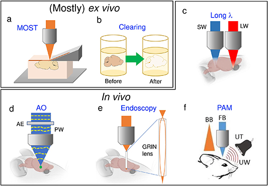
Figure 2. Summary of methods to enhance imaging depth. Schematic illustration of the principles of (a), (b) Ex vivo imaging: (a) micro optical sectioning tomography (MOST), and (b) tissue clearing; as well as (c)–(f) In vivo imaging: (c) long wavelength, (d) adaptive optics (AO), (e) endoscopy, (f) photoacoustic microscopy (PAM). SW: short wavelength, LW: long wavelength, AE: adaptive element, PW: pre-aberrated wavefront, GRIN: gradient-index, UW: ultrasound waves, UT: ultrasound transducer, BB: broad beam, FB: focused beam. Mouse brain figures are adopted from the BioRender website.
Download figure:
Standard image High-resolution imageThe serial sectioning tomography concept has also been combined with 2PE microscopy [144, 145], to enable whole mouse brain connectome study [146]. In Drosophila, the idea of whole body connectomics was demonstrated, together with novel neural simulation tools [147]. In 2017, block-face serial microscopy (FAST) [148] was developed to significantly enhance the imaging speed, and to enable neuronal circuit mapping in a whole brain of a non-human primate marmoset as well as in a part of a post-mortem human brain.
One major challenge of MOST, and other similar serial sectioning based methods, is to keep connection integrity during slicing, so careful sample preparation design is critical [149]. In the next section, we introduce optical clearing, which can significantly enhance imaging depth of an intact organ or even whole animal without physically cutting the sample.
3.2. (Mostly ex vivo ) Tissue clearing
Tissue clearing techniques improve imaging depth by making the biological specimen transparent via dramatically reducing light scattering, as shown in figure 2(b). The neuroscience community recently witnessed an explosive growth in clearing methods, summarized in an up-to-date review [150]. These methods greatly extend visible light imaging depth toward not only the whole brain, but also the whole animal. Currently, there are three major directions of tissue clearing: solvent-based, aqueous-based, and hydrogel-based. In the following, we briefly describe their clearing capabilities, fluorescence maintenance, volume variation, processing time, and reversibility.
Solvent based clearing methods have been developed for more than 100 years [151], with three major steps including dehydration, lipid removal, and refractive index matching. The techniques are conventionally compatible with chromogenic H&E or metallic Golgi staining, but one major challenge is that dehydration significantly diminishes fluorescence, in particular for fluorescent proteins. Contemporary solvent techniques, such as various versions of 3D imaging of solvent-cleared organs [152–156], enable nearly full transparency in a whole mouse brain, a whole mouse and even a complete human embryo, as well as stabilize the endogenous fluorescent signal. The clearing process typically takes a few hours. It is important to note that solvent-based methods are not reversible, and may shrink the sample size by ∼50%, posing another important challenge to ensure the spatial accuracy of 3D histological structures.
Aqueous-based methods use water-soluble reagents, which form hydrogen bonds with tissue components for refractive index matching, thus providing high levels of biocompatibility, and preservation of fluorescent protein. One representative example is FocusClear, which was demonstrated by Ann-Shyn Chiang nearly 20 year ago [157]. FocusClear can make an insect brain completely transparent within minutes, as well as maintain dye or protein fluorescence with minimal loss. More importantly, the clearing process is reversible, and does not alter the specimen size. The main limitation of FocusClear is its applicability to large samples [158], such as a whole mouse brain. Alternatively, Scale [159, 160] based on urea can clear the whole mouse brain and provides the best fluorescence retention [161]. Nevertheless, tissues in Scale take long incubation time to clear and swell significantly. In general, FocusClear provides better transparency than Scale for small tissues, such as the fly brain.
The third category is hydrogel-based techniques, and a representative example is CLARITY [162], which applies electrophoresis to remove lipids, creating a hydrogel to keep the protein and DNA integrity. It is interesting to note that after electrophoresis, FocusClear is used in CLARITY to make tissue more transparent and maintain fluorescence, thus allowing entire mouse brain imaging via light sheet microscopy. Typically, it takes days to weeks to clear a whole mouse brain, and during electrophoresis some proteins may be lost. Various improvements of CLARITY appeared soon after the first paper, such as passive CLARITY that enabled impressive whole body clearing of a mouse [163], and bone CLARITY that allowed intact bone marrow observation [164]. During the hydrogel processing, the specimen volume may slightly expand, inspiring the idea of expansion microscopy (see section 4.3).
The above clearing methods are applicable only to ex vivo tissues. In vivo clearing methods to reduce the scattering of skin [165, 166] and skull [167] have been developed. In these studies, glycerol is used to match the refractive indices of (collagenous) tissues, so fluorescence is not affected significantly, with no appreciable volume variation. Impressively, the pioneering skull-clearing method, together with two-photon microscopy, offers at least 250 μm imaging depth into the brain pial surface, and is fully reversible. Interested readers are referred to two recent reviews that nicely summarized current state-of-the-art in vivo results [168, 169].
In the above two sections, i.e. MOST and tissue clearing, imaging depth increases via sample processing, so it may alter intrinsic structures. In the following, we address optical techniques that enhance penetration depth and allow in situ and in vivo imaging of brain tissues, including long wavelength modalities, AO, endoscopy, and photoacoustic microscopy.
3.3. (In vivo) Long-wavelength emission/excitation
Imaging depth in a living brain is generally limited due to light attenuation, include scattering and absorption. Since long-wavelength light exhibits less scattering [136, 170], a typical deep imaging strategy is to select long wavelength excitation/emission which avoids water absorbance. For example, by adopting carbon nanotubes whose excitation is at 808 nm and emission at 1300–1400 nm, more than 2 mm imaging depth through an intact skull in a living mouse brain was demonstrated [171].
However, most fluorophores used in brain imaging emit visible light, hence, long-wavelength excitation through multiphoton absorption should be adopted. Multiphoton microscopy provides noninvasive deep-tissue imaging, allows localized excitation in 3D, and exhibits less photobleaching and phototoxicity. The typical imaging depth of a 2PE microscope based on a Ti:sapphire laser is ∼0.6–0.8 mm (section 2.2), much deeper than 1PE in the mouse brain cortex [136]. Therefore, multiphoton techniques have gained a special niche for thick-tissue volumetric imaging.
To further increase imaging depth, several strategies have been developed. One is increasing the Ti:sapphire laser pulse energy, demonstrating ∼1 mm imaging depth in a mouse brain [172]. However, high-energy pulses may induce multiphoton ionization and photodamage. Other strategies adopt long wavelength, high nonlinearity, or the combination. By using a ∼1300 nm excitation source, we have demonstrated third-harmonic generation imaging at 1.5 mm depth in a developing zebrafish embryo [173], and Chris Xu has demonstrated in vivo 2PE imaging up to 1.6 mm depth in a mouse brain [174]. By employing an excitation source at ∼1700 nm, 2PE further pushed imaging depth to 2 mm in vivo [175]. Recently, three-photon microscopy with 1300 nm or 1700 nm excitation wavelength also achieved comparable imaging depth [176, 177], but offers better optical section ability, enabling through-skull and transcutical in vivo imaging in mice and Drosophila, respectively [178, 179]. According to our recent analysis [138], aberration is the main limiting factor of three-photon imaging depth in a Drosophila brain. Therefore, for whole-brain in vivo imaging, three-photon microscopy with AO, which compensates aberrations, shall be the most promising way [180].
3.4. (In vivo) AO
Due to inhomogeneous refractive index in biological tissues, the optical wavefronts of both illumination and emission beams are distorted, i.e. optical aberration, resulting in reduced resolution and image contrast. It is well known that the major factor that limits imaging depth is signal-to-background ratio, which degrades in deep tissue due to PSF broadening via scattering and aberration [181]. Scattering may be reduced by long wavelength excitation/emission (section 3.3). To overcome aberration, one possible method is tissue clearing (section 3.2), which may alter the natural sample status. The optical approach to compensate for aberration is through AO, a technique borrowed from astronomical telescopes [182]. Its fundamental working principle is to pre-aberrate the wavefront to compensate for the aberration induced by the specimen/optical system, as shown in figure 2(d). For more details on AO microscopy, we refer the readers to recent comprehensive reviews [183, 184]. Essentially, an AO system is composed of two parts: one for wavefront correction and the other for wavefront characterization, that we briefly introduce below.
For AO wavefront correction in the field of optical microscopy, liquid crystal SLM (LCSLM) [185] or DM [186] are mostly applied. The former offers more complexity in wavefront manipulation, and the latter has higher refresh rates with robust operation independent of polarisation and wavelength. More recently, a plug-and-play multi-actuator adaptive liquid lens is adopted to significantly reduce the setup intricacy and can be applied to commercial microscopes directly [187].
Regarding wavefront characterization, which is necessary to achieve optimal compensation, there are direct and indirect methods. The direct method typically relies on a Shack–Hartmann sensor, composed of a lens array and a camera, to visualize the distorted wavefront from 'guide stars' inside tissues [188]. The indirect one, aka the sensorless method, is based on either iterative optimization of image contrast through Zernike wavefront decomposition [189] or pupil segmentation [190].
In biological tissues like brains, the most commonly encountered aberrations are low-order Zernike modes like spherical aberration, coma, and astigmatism due to index inhomogeneity [191]. Spherical aberrations, as one of the most common aberrations from sample/medium refractive index mismatch, had been extensively studied long before the first adaptive microscope [183]. When various wavefront distortions are effectively corrected by AO systems, image signal-to-background ratio, as well as imaging depth, is improved.
In optically transparent samples, where aberration still exists, AO has shown to recover diffraction-limited images in depth over 270 μm [192]. To extend this approach, near-infrared guide stars are utilized to reduce scattering, enabling high-contrast 2PE imaging down to 700 μm inside the mouse brain [188]. More recently, via microvascular-based near-infrared guide stars, near-diffraction-limited 2PE imaging up to 850 µm in awake mice is achieved, enhancing the signal around 2–3 folds [193]. Furthermore, AO can be integrated in three-photon microscopy to improve image quality up to 1 mm [194].
3.5. (In vivo) Endoscopy
To increase imaging depth, sections 3.1 and 3.2 consider invasive methods of MOST and clearing, while sections 3.3 and 3.4 address non-invasive methods of long wavelength excitation and AO. In this section, we introduce a partially invasive method, optical endoscopy, which may achieve centimeter imaging depth, while maintaining subcellular spatial resolution. Endoscopy observes the inner part of an organ via inserting thin imaging probes, including multicore fiber bundles, a single-mode fiber, a double-cladding fiber, a multi-mode fiber (MMF), or a gradient-index (GRIN) lens [195, 196]. Here we mainly focus on multiphoton endoscopy, where the GRIN lens and MMF were adopted in most cases for volumetric in vivo imaging of the brain, as shown in figure 2(e).
GRIN-lens-based multiphoton endoscopy was first demonstrated in 2003, with a GRIN lens of 1–2 cm length, i.e. the reachable imaging depth, in a zebrafish brain [197], and later in a mouse brain [198, 199]. An amazing case with unprecedented imaging depth uses a 28.5 cm long GRIN lens for two-photon imaging of unstained tissue, manifesting that multiphoton endoscopy for a human brain might be possible [200]. The 3D spatial resolution of multiphoton endoscopy can be improved when the intrinsic aberration of the GRIN lens is corrected [201].
More recently, GRIN lens is combined with various multiphoton volumetric approaches that we introduced in section 2. For example, Moretti et al used phase modulation to efficiently project complex 2PE patterns in the focal plane of a GRIN lens, performing scanless functional volumetric imaging (cf section 2.1.5) at ∼1.2 mm depth in rodent hippocampal networks in vivo [202]. Sato et al presented a fast varifocal two-photon microendoscope system equipped with a GRIN lens and an ETL (cf section 2.2.2) [203], enabling quasi-simultaneous neuronal activity mapping of two deep-brain focal planes separated by 85–120 µm at ∼10 fps. In 2019, Meng et al incorporated a Bessel focus scanning module (cf section 2.2.2) into two-photon fluorescence microendoscopy, with lateral resolution improved, to observe mouse hippocampus and lateral hypothalamus in vivo [204]. In the open source 'Miniscope' project, the latest development is to optimize light-field acquisition (cf section 2.1.3) to achieve 40 fps 3D brain imaging in freely-moving animals [205]. In 2021, we combined TAG lens (section 2.2.2) and a GRIN lens to observe calcium dynamics in suprachiasmatic nuclei, which is located at the bottom of a mouse brain [206].
Apart from the GRIN lens with nearly mm diameter, a hair-thin MMF with ∼100 μm diameter serves as a much less invasive endoscopic device. In the past, MMF was mainly used to deliver light instead of image acquisition. Thanks to recent advances in wavefront shaping that allows proper focusing after an MMF, MMF-based multiphoton endoscopy was realized [207–209], and fast volumetric imaging has also been achieved [210, 211]. The main drawback of MMF endoscopy is its limited FOV, which may improve via novel AO approaches [212].
3.6. (In vivo) Photoacoustic approaches
The dream of in vivo brain imaging is to reach the whole brain depth, say centimeter scale, and maintain cellular spatial resolution and tissues intact, i.e. without the need of skull and scalp removal. Photoacoustic imaging is a potential candidate toward this goal. The essence of photoacoustic imaging is a combination of optical excitation and acoustic detection, as illustrated in figure 2(f), which allows in vivo label-free imaging of the brain [213, 214]. In photoacoustic imaging, biological tissues are excited using broad or focused laser beams with appropriate wavelengths to the targeted optical absorbers, e.g. hemoglobin. The optical absorbers absorb and then convert the laser energy into ultrasound waves via thermoelastic expansion. The photoacoustic image with high optical absorption contrast is then formed with the detected ultrasound. Leveraging optical absorption contrast and relatively weak acoustic attenuation and scattering (compared with optical ones) in biological tissues, photoacoustic imaging has been demonstrated to be capable of performing real time morphological, functional and molecular imaging of living subjects with high contrast and centimeter-scale penetration [215, 216].
Since Wang et al reported the first photoacoustic imaging work on in vivo noninvasive transdermal and transcranial imaging of the structure and function of rat brains, photoacoustic imaging has gained growing attention in brain imaging [217]. Photoacoustic brain imaging nicely complements the drawbacks of other deep brain imaging modalities, e.g. poor depth-to-resolution ratio in diffusive optical tomography and low temporal resolution in MRI. The spatial resolution, imaging depth, and functional capability of the photoacoustic brain imaging mainly depends on the configuration of laser excitation and acoustic detection.
With excitation of broad laser beams, two types of photoacoustic imaging—photoacoustic tomography (PAT) and acoustic resolution photoacoustic microscopy (ARPAM) are proposed. In PAT and ARPAM, because the absorbed photons are localized ultrasonically, the en face and axial spatial resolution is limited by acoustic diffraction and detector bandwidth, respectively, ranging from few tens to few hundreds of micrometers. Generally, PAT is equipped with low frequency ultrasound transducers (e.g. <10 MHz) and can offer > 5 cm penetration because low frequency ultrasound suffers less attenuation [216]; ARPAM using high frequency transducers (e.g. >20 MHz) can provide 1 cm penetration. Though there is trade-off between the penetration and spatial resolution in PAT and ARPAM, depending on the detected ultrasound frequency, the depth-over-resolution ratio of both PAT and ARPAM is larger than 100, indicating that PAT and ARPAM are still high resolution imaging techniques [213]. The uniqueness is that with endogenous hemoglobin contrast, PAT and ARPAM can image dynamic changes of multi-neurovascular-coupling parameters independently, such as total hemoglobin concentration, cerebral blood volume, and cerebral blood oxygenation, in single blood vessel level over the whole rat and mouse brain without the need of skull removal [218, 219]. With endogenous contrast, e.g. genetically-encoded probes plus calcium dependent absorption spectra, PAT can offer deep molecular imaging of neural activity [220, 221].
On the other hand, with focused-beam excitation, optical resolution photoacoustic microscopy (ORPAM) has been developed. With optical focusing, the en face spatial resolution of ORPAM corresponds to the optical diffraction limit, reaching ∼1 μm and even sub-micrometer while the imaging depth is compromised to within one-transport mean free path, i.e. ∼1 mm. Moreover, because of the acoustic detection nature, the axial resolution of ORPAM is still limited by acoustic detection bandwidth, which is about few tens of micrometers when a 50 MHz high frequency transducer is used [213]. Combining blood flow information with the multi-neurovascular-coupling parameters mentioned above, it has been demonstrated that ORPAM is capable of transcranial cortical imaging of cerebral metabolic rate of oxygen in single micro-vessel level in mouse brains with endogenous hemoglobin contrast [222]. ORPAM also has shown its capability of trans-cuticle brain imaging of Drosophila with exogenous fluorescence protein because of the low acoustic attenuation of the cuticle [223].
With centimeter-scale penetration and high spatial resolution, moving toward PAT human brain imaging is the most exciting and challenging research direction [224]. Although the optical and acoustic attenuation of the thick human skull significantly degrades the PAT human brain imaging quality, significant progress is expected in coming years [225].
To conclude section 3, we summarized the performance of depth-enhancing techniques in table 2. Starting from techniques that are mostly applied to ex vivo brain tissues, i.e. MOST and tissue clearing, the imaging depth of the former is in principle unlimited, and the latter can achieve at least whole mouse body clearing. MOST maintains the spatial resolution throughout the sections, and may achieve depth-over-resolution ratio above 10000. When combined with super-resolution modality, the ratio exceeds 100 000! However, for large samples, it is time consuming and faces the difficulty of maintaining sophisticated connections. Optical clearing may preserve the neural patterns, whereas in a large tissue, the spatial resolution is degraded with depth. Combining the advantage of these two methods would enable whole brain/animal neural structure mapping with best optical resolution and intact fiber structures.
Table 2. Comparison of various deep imaging modalities. The depth/resolution numbers presented here refer to mouse samples. For other sample types, please see the main text.
| Methods | Depth | Resolution | Depth/resolution | Invasive | Reference |
|---|---|---|---|---|---|
| MOST | Whole-brain | 0.7 μm | > 10000 | Yes | [148] |
| MOST + STED | 0.06 μm | > 100 000 | |||
| Tissue clearing | Whole-brain | <1 μm a | > 10000 | Mostly yes | [161, 163] |
| Long-wavelength (nm) | |||||
| 1PE (ex 808; em 1300–1400) | ∼2 mm | <10 μm | > 200 | [171] | |
| 2PE (ex 1617; em 814) | ∼2 mm | <5 μm | > 400 | No | [175] |
| 3PE (ex 1700; em 584) | ∼1.3 mm | <1 μm | ∼1000 | [177] | |
| Adaptive optics | ∼1 mm | <1 μm | ∼1000 | No | [54] |
| Endoscopy | >cm | <1.5 μm | ∼10000 | Yes, but in vivo | [204] |
| Photoacoustic | |||||
| PAT | 48 mm | 125 μm | 400 | [216] | |
| ARPAM | 4 mm | 70 μm | ∼100 | No | [213] |
| ORPAM | 0.75 mm | 3 μm | ∼250 | [222] |
a As mentioned in reference, but may be worse when imaging deep in the cleared brain.
For in vivo methods, long-wavelength excitation in the biological transparent window provides 1–2 mm penetration depth together with <1 μm spatial resolution, achieving depth-over-resolution ratio above 1000. Combining with AO instruments, the image contrast, as well as spatial resolution, can be further enhanced. Although the contrast enhancement should lead to significant depth enhancement, currently this potential has not been fully utilized, and imaging depth of noninvasive optical microscopy is limited to mm-scale. To further enhance depth, a different contrast based on photoacoustic detection may be adopted, providing multi-scale imaging capability, from whole-mouse imaging with 100 μm resolution, to 1 mm depth with 1 μm resolution (similar to pure optical imaging).
Overall speaking, for noninvasive optical imaging modalities in table 2, resolution degrades as imaging depth increases, leading to depth-over-resolution ratios of a few hundreds to one thousand. This trade-off between depth and resolution is well documented in literature [226, 227]. As shown in table 2, invasive methods, such as MOST and clearing, break the trade-off, but sacrifice the in vivo observation ability. The partially invasive method, endoscopy, breaks the trade-off by offering penetration depths larger than 1 cm and spatial resolution around 1 μm, while maintaining in vivo imaging capability. In the future, innovative in vivo clearing methods may bring breakthroughs in this field. Another potential candidate to achieve in vivo observation while breaking the resolution-depth trade-off is artificial intelligence. Through a training set consisting of volumetric blurred and high-resolution serial images, deep-tissue resolution may be considerably enhanced [228]. This is currently feasible only for ex vivo imaging. Applying deep-learning to in vivo imaging may lead to artifacts due to previously unknown patterns.
It is important to note that the depth-resolution trade-off exists not only within optical imaging, but is a general phenomenon across different imaging modalities. For example, medical imaging modalities such as MRI, computed tomography, positron emission tomography, and ultrasound, have human-body penetration capability, but their resolutions are generally at submillimeter to millimeter scale. Optical imaging modalities such as optical coherence tomography and diffuse optical tomography offer 1–10 cm depth, but the resolutions are not adequate to resolve cells. EM has nanometer resolution, yet it is limited to surface or ultrathin slice imaging. By further studying and comparing physical origins of depth-resolution limitation among different techniques, new ideas of optical imaging might emerge. For example, the resolution of MRI is determined by magnetic field gradient, not affected by tissue scattering, and reaches two orders smaller than its radio-frequency electromagnetic wavelength. This may be an inspiring example for optical imaging to break the diffraction limit in scattering tissues, which is the topic of next section.
4. Review of super-resolution imaging in deep tissue
Delineating subcellular structures such as synapses in a neuronal network is a major goal of brain study because it provides direct evidence of neural connections and gives hints of underlying interactions. The size of synaptic vesicles is ∼40 nm, which is not resolvable by conventional optical microscopy. Due to diffraction of light, the optical resolution is limited to λ/2, i.e. ∼200 nm with visible excitation. One major breakthrough in the 21st century is the development of super-resolution techniques [229], which ameliorate resolving power down to tens of nanometers, even approaching 1 nm recently [230]. Most present super-resolution modalities are limited to cellular imaging with negligible scattering/aberration. Here we concentrate on recent developments of tissue-compatible super-resolution techniques.
Fundamentally, the resolution limit could be surpassed by leveraging other properties of emitted signals, such as time, polarization, wavelength, etc [231]. The classic example is to turn on fluorescence molecules 'deterministically' (through wavefront engineering) or 'stochastically' (through fluorophore dynamics) in time, and to localize their spatial coordinates by computational post processing. A different approach that was invented recently is to physically 'expand' the tissue, thus effectively enhancing spatial resolution. In the following, we introduce recent developments based on these three concepts (deterministic, stochastic, and expansion), with a special emphasis on speed (section 2) and imaging depth (section 3), toward realizing high-speed whole-brain super-resolution imaging.
Please note that our aim here is to address the link between super-resolution methods and volumetric imaging of the brain, so we are not going to explain in detail the technical background of each technique. Readers who are not familiar with super-resolution imaging are encouraged to read relevant articles, e.g. an comprehensive review published in Journal of Physics D by Hell et al [232]
4.1. Deterministic super-resolution imaging in deep tissue
The deterministic method features a patterned excitation to selectively turn 'on' the molecules. Notable examples of deterministic methods include stimulated emission depletion (STED) [233], reversible saturable optical fluorescence transitions (RESOLFT) [234], excitation nonlinearity [235], and structured illumination microscopy (SIM) [236], that we are going to discuss respectively below.
4.1.1. STED/RESOLFT.
A characteristic of STED and RESOLFT microscopies (figure 3(a)) is the need of two illumination beams: one for excitation and the other for inhibition. The inhibition beam, which is donut-shaped, turns 'off' peripheral fluorescence emission and confines the excitation of fluorophores ('on' state) in a small volume, achieving ∼20 nm resolution in live cell imaging [237–239]. Three dimensional super-resolution microscopies are also developed for live brain imaging and its resolution is ∼60 nm laterally and ∼150 nm axially [240, 241]. Similar resolution enhancement via confinement of emission can also be achieved by non-fluorescent nanomaterials, such as absorption of graphene [242] and scattering of gold nanoparticles [243].

Figure 3. Summary of super resolution imaging in deep tissue techniques. Schematic illustration of the principles of (a)–(c) deterministic super resolution imaging: (a) STED microscopy, (b) excitation nonlinearity, and (c) SIM; (d), (e) stochastic super resolution imaging: (d) principles of STORM and PALM, (d1) with LSM, (d2) with temporal focusing excitation (TF), (d3) with spinning disk confocal excitation (SDCM), and (e) SELFI. (f) expansion microscopy. IB: inhibition beam, EB: excitation beam, L: linear, NL: nonlinear, Emi: emission, Exc: excitation, G: grating.
Download figure:
Standard image High-resolution imageFor tissue imaging, aberration and scattering distort the donut inhibition beam, thus deteriorating super-resolution. As mentioned in section 3, imaging depth can be significantly enhanced by reducing aberration and scattering. By correcting spherical aberration with objective correction collar, STED achieves 70 nm resolution at 120 μm depth in organotypic brain slices [244]. Through reducing scattering via long-wavelength excitation, two-photon STED demonstrated 60 nm resolution at 50 μm depth in acute brain slices [245, 246]. Combining STED with a hollow Bessel beam, which is less susceptible to scattering, provides >100 μm imaging depth in a phantom. Although the same strategies should all be applicable to RESOLFT [247], the reported imaging depth of RESOLFT to date is only about 30 μm [248].
4.1.2. Excitation nonlinearity.
A well-known approach to enhance spatial resolution for tissue imaging is through nonlinear optical responses. For example, two-photon and three-photon microscopy enhances spatial resolution by a factor of √2 and √3, due to the quadratic and cubic power dependency, respectively. However, typically multiphoton microscopy adopts a near-infrared excitation source, to enhance penetration depth, so the resolution gain is compensated with long wavelength. Interestingly, combining 2PE with a visible laser, Oketani et al has shown resolution better than single-photon excitation [249].
Instead of the conventional nonlinear optical responses, even under single photon excitation, the emission and excitation power dependency are not always linear. A well-known nonlinear property of fluorescence is saturation under intense excitation. Saturated excitation (SAX) microscopy, developed by Fujita et al in 2007, enhances spatial resolution via extracting the saturated part, and is capable of discerning actin filament in a 3D cell matrix in 40 µm depth [250]. Two-photon SAX has achieved a 100 μm penetration depth with 1.3-fold resolution enhancement [251].
Recently, we have found that the scattering of gold/silicon nanoparticles exhibit nonlinear responses, including saturation and reverse saturation, that enables significant resolution enhancement [252–254]. A novel combination of plasmonic scattering saturation with SAX realized three-fold resolution enhancement across a ∼200 μm thick tissue [255]. Furthermore, the saturation of upconversion nanoparticle emission leads to 50 nm resolution at 93 μm depth [256].
4.1.3. Structured illumination microscopy (SIM).
SIM enhances spatial resolution, maximally two-fold [236, 257], via mathematical deconvolution of sparse Moiré-fringes-like signals from the convolution of fluorescent signals and multiple high-frequency structured illuminations, as depicted in figure 3(c). Combining fluorescence saturation, saturated-SIM allows theoretically unlimited resolution (50 nm demonstrated) [258]. Similarly to STED, the structured illumination is susceptible to aberration and scattering, so it is challenging to implement SIM in tissues [259]. A combination of SIM and temporal focusing has shown a 1.6-fold enhanced lateral resolution at 160 μm depth with fluorescent beads in agarose [260]. A recent work combining two-photon laser scanning microscopy with SIM (2pSIM) demonstrated 120 nm resolution at 120 μm depth in a living mouse brain [261].
In a brief summary, deterministic super-resolution methods enable sub-100 nm resolution at depth ∼100 µm in brain tissues, i.e. depth-over-resolution ratio above 1000, at a speed similar to laser scanning microscopy. Nevertheless, it is challenging to further enhance spatial resolution. Below we address stochastic super-resolution methods, which is typically much slower than deterministic methods, but with better resolution.
4.2. Stochastic super-resolution imaging in deep tissue
When adjacent fluorophores emit simultaneously, as in conventional microscopy, they are not resolvable. However, if they emit 'stochastically', leveraging fluorescence information accumulated within hundreds of frames, allows to localize the spatial coordinate with a precision up to 10 nm. The resolution enhancement is obtained through fitting the center of emission PSF (sparsely). This is the underlying principle of stochastic super-resolution imaging techniques, presented in figure 3(d). There are many different variants, just to name a few well-known examples like stochastic reconstruction microscopy (STORM) [262], photoactivated localization microscopy (PALM) [263], and DNA point accumulation for imaging in nanoscale topography (DNA-PAINT) [264]. They are all based on wide-field detection schemes, so to achieve tissue imaging, it is necessary to incorporate optical sectioning techniques (cf section 2.1), such as LSM and LLSM in figure 3(d1) [265, 266]. Adding long-wavelength excitation and two-photon excitation with LSM plus PALM, 40 nm resolution is achieved in a 150 μm thick agarose scattering phantom [267]. Stochastic super-resolution has also been combined with single-objective LSM with oblique illumination, and demonstrated 40 nm resolution at 40 μm depth in mouse brain slices [268].
In principle, all the camera-based volumetric imaging techniques in section 2.1 should be compatible with stochastic super-resolution. For example, temporal focusing has been combined with PALM (figure 3(d2) [269]); SDCM has been combined with DNA-PAINT (figure 3(d3) [270]) to significantly improve the spatial resolution. However, these reports used cell samples, so the demonstrated imaging depth is below 10 µm. An innovative approach based on fluorescence self-interference (SELFI) to capture the emitter's axial position allows impressively 40 nm isotropic resolution at 50 μm depth of stem cell organoids [271].
As mentioned in section 3.2, one strategy to significantly enhance penetration depth is through optical clearing. A notable example is light-sheet localization microscopy for clarified tissue (LLM-CT), where the whole Drosophila brain can be mapped with 50 nm resolution within 1 day [272]. This is orders-of-magnitude faster than EM [4]. Confocal localization deep imaging with Optical clearing (COOL), a technique combining SDCM and tissue clearing, can achieve 20 nm resolution (localization uncertainty) across the whole Drosophila brain (∼200 µm) [273], i.e. achieving depth-over-resolution ratio of 10 000.
4.3. Expansion microscopy
Expansion microscopy, differently from other techniques which exploit the illumination or detection modification, enhances spatial resolution via isotropic physical expansion of biological tissues [274], schematically shown in figure 3(f). The technique is a combination of hydrogel clearing (cf section 3.2) and the physics of swellable polyelectrolyte hydrogels. The former allows preservation of tissue staining, while the latter offers significant resolution enhancement (typically 4× to 10×) with conventional microscopes [275]. With 10× expansion, the attainable resolution is about 20 nm, which is comparable to other super-resolution techniques. However, the limitation arises from the working distance and numerical aperture (NA) trade-off, which is similar to the general trade-off between penetration depth and resolution that we discussed in the last two paragraphs of section 3. When a high NA objective is adopted to enhance the spatial resolution, the working distance is often short. For example, a 40 × 1.15 NA water-immersion objective has 600 µm working distance. When using this objective with a 20-fold iterative expanded sample, the effective imaging depth is merely 30 µm before expansion [276]. By contrast, a four-fold magnified analysis of the proteome, a similar version of expansion microscopy without protease treatment, adopts a low NA (0.6) long working distance (8 mm) objective but the resolution degrades quickly in the tissues deeper than 100 µm due to the inherent aberration [277]. Currently, the-state-of-the-art expansion microscopy for super-resolution imaging works only for small-animal brains, such as a whole Drosophila brain with 60 × 60 × 90 nm resolution at 4× expansion [35]. For large samples, either sectioning should be conducted before imaging (section 3.1) or imaging at low magnification under the new Mesolens with long-working distance and high NA is utilized [278].
4.4. High-speed super-resolution volumetric imaging
This review has covered imaging speed in section 2, depth in section 3, and resolution enhancement in section 4. In sections 4.1–4.3, we reviewed recent advances of super-resolution imaging in thick samples, i.e. addressing the factors of resolution and imaging depth. Now in this section, we further consider the factor of imaging speed, toward the vision of high-speed super-resolution volumetric imaging in brain.
For deterministic approaches, which mostly rely on point scanning, the techniques that we addressed in section 2.2, including multiplexing and high-speed scanning, shall be applicable to improve the speed. The first spatially multiplexed STED and RESOLFT were both developed by Stefan Hell's group [279, 280]. High-speed scanners such as an electro-optical scanning (>1000 frame s−1) was combined with STED to enable high-speed tracking of vesicles with <10 ms temporal resolution [281]. A very recent work combining electro-optical scanning and multiplexing shows promising millisecond STED imaging over large fields of view [282]. On the other hand, the axial resolution (but not lateral resolution) of high-speed light sheet microscopy can be enhanced by one order of magnitude via combination with RESOLFT [283] and STED [284].
For stochastic super-resolution methods, the speed limitation is due to the requirement of accumulating hundreds of frames. Artificial neural networks, by requiring its powerful image recognition capability [285], accelerate super-resolved image reconstruction with two-order less raw images [286] or with faster computation [287]. With accumulation of large pre-training dataset, even a single diffraction-limited image can be transformed into a super-resolution image after a deep learning neural network [288]. Nevertheless, it may be difficult or time-consuming to prepare a large training dataset.
For expansion microscopy, in principle, all the high-speed modalities mentioned in section 2 can be applied. As we mentioned earlier, the combination of expansion microscopy and lattice LSM (ExLLSM) [35] provides synapse-level resolution over an entire Drosophila brain within a few days. It is interesting to notice that LLM-CT (section 4.2) is superior both in terms of spatial resolution and speed. We envision that the combination of stochastic super-resolution microscopy, light sheet illumination, and expansion sample processing may provide ultimate performance in resolution, speed, and imaging depth, pushing toward the circuit visualization of not only mammalian brains, but even a complete human brain, down to synaptic level. Note that serial sectioning may be required for such large samples, and currently expansion (or optical clearing) is not compatible with living brains.
To conclude this super-resolution section, a comparison of aforementioned super-resolution techniques is presented in table 3 and figure 4. Although the performance (e.g. resolution, depth, etc) of each technique is sample-dependent, it is interesting to note that in general, deterministic techniques (STED, nonlinearity, and SIM) provide faster speed, i.e. less than 1 s acquisition time per FOV, and less spatial resolution of 60 nm or above; stochastic methods (STORM, PALM, DNA-PAINT, and SELFI) have superior resolution around 20 nm, but take more than 100 s to accumulate enough frames for a single reconstructed FOV, implying a trade-off between speed and resolution. Expansion microscopy is between these two categories, nevertheless its sample preparation may be more time-consuming.
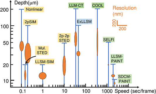
Figure 4. A summarized figure comparing resolution (orange circles), imaging depth, and imaging speed for techniques in table 3. Yellow, green and blue colors represent deterministic, stochastic, and expansion modalities, respectively. Please note that the performance of different super-resolution imaging techniques is sample-dependent. This figure shows the reported data according to the references listed in table 3.
Download figure:
Standard image High-resolution image
Table 3. Comparison of various super resolution imaging in deep tissue techniques modalities. It is interesting to compare the depth/xy resolution column with table 2, though sample type may be different.
| Methods | xy res. (nm) | z res. (nm) | Depth (μm) | Depth/xy res. Ratio | Second/FOV | Sample | Reference |
|---|---|---|---|---|---|---|---|
| Deterministic | |||||||
| 2p–2p STED | ∼60 | ∼1000 | 50 | ∼830 | ∼10 | Mouse brain | [245, 246] |
| Multiplex STED | ∼35 | ∼500 | ∼20 | ∼570 | 0.2 | Cell | [279, 282] |
| Nonlinear | ∼80 | ∼500 | 200 | ∼2500 | ∼0.1 | Chicken breast | [255] |
| 2pSIM | 120 | ∼1000 | 120 | ∼1000 | ∼0.3 | Mouse brain | [261] |
| LLSM-SIM | ∼150 | ∼280 | 20 | ∼130 | ∼1 | Embryo | [34] |
| Stochastic | |||||||
| LLSM-PAINT | ∼70 | ∼100 | 20 | ∼290 | ∼2500 | Zebrafish | [266] |
| SDCM-PAINT | ∼20 | ∼80 | 10 | ∼500 | ∼3000 | HeLa cell | [270] |
| SELFI | ∼20 | ∼20 | 50 | ∼2500 | ∼1000 | Spheroid | [271] |
| LLM-CT | ∼20 | ∼550 | 200 | ∼10 000 | ∼50 | Cleared fly brain | [272] |
| COOL | ∼20 | ∼1000 | 200 | ∼10 000 | ∼500 | Cleared fly brain | [273] |
| Expansion | |||||||
| ExLLSM | ∼60 | ∼90 | ∼100 | ∼2000 | ∼600 | Fly/mouse brain | [35] |
Another common trade-off in the field of optical microscopy is between depth and resolution, as mentioned in the conclusion of section 3 (table 2). Here in table 3, the ratio between depth and xy resolution is presented for quantitative comparison of different super-resolution imaging modalities. These ratios of most techniques are on the order of 1000, similar to that of noninvasive techniques in table 2, manifesting the ubiquitous depth-over-resolution trade-off. In table 3, LLM-CT and COOL rely on tissue clearing (section 3.2), leading to one order enhancement of depth-over-resolution performance. Interestingly, table 2 also displays a similar depth-over-resolution enhancement via clearing. When considering 3D resolution, SELFI features the smallest 3D PSF, as well as highest depth-over-PSF-volume ratio, and more importantly, it is feasible for in vivo imaging, though the speed is slow. More technical innovations are highly desirable toward the goal of in vivo whole brain imaging at 10–20 nm spatial resolution.
5. Discussion
Understanding the brain is one of the most significant scientific problems in our era. Conventionally, most efforts toward this problem lie in mapping the anatomical structures, such as the FlyCircuit from the Brain Research Center of National Tsing Hua University in Taiwan, the Mouse Brain Atlas from the Allen Institute for Brain Science, the Non-Human Primate Atlas (rhesus macaque) from NIH, and the human brain atlas from the Human Brain Project of EU [289–292]. In particular, the Flycircuit database contains high resolution confocal images of more than 60000 neurons, i.e. covering more than half total neurons in a Drosophila brain. The covering ratio is much more than all other model animals, making Drosophila an ideal animal to understand the whole-brain emergent properties. Nevertheless, the ultimate goal is certainly to unravel the mystery of the human brain, so it is highly desirable to study the brains of mice and monkeys, which are more similar anatomically than Drosophila.
As we mentioned in the introduction, the above anatomical mappings only reveal the 'hardware' connectivity of the brain, but to understand how a brain functions, the key ingredient should be the 'software'. Functional imaging, still observing hardware connectivity, opens a valuable window into the underlying software along three directions: (a) capturing information flow, (b) accessing the whole brain, (c) resolving individual neurons/synapses. In this review, section 2 is devoted to address direction (a) through introducing high-speed volumetric optical imaging for brains, i.e. advancing temporal resolution to register sub-second ionic dynamics and millisecond action potential propagations. In section 3, which aims for direction (b), we mention methods for pushing imaging depth from millimeter scale (Drosophila, zebrafish brains) toward centimeter scale (mouse/rat brains), in order to obtain emergent properties from connectivity across a whole brain, or at least across brain regions. For direction (c), it is highly desirable to observe not only functional transduction among intricate synaptic interconnectivities, but also vesicles and neurotransmitters in action, whose physical size is far below optical diffraction limit, in a living brain. Therefore, in section 4, super-resolution methods that are compatible with tissue volumetric modalities are introduced, advancing the ratio between depth and resolution up to 200 μm/20 nm = 10 000. Nevertheless, the above results have mostly been demonstrated only in small model animals.
To apply optical microscopy for in vivo human brain imaging, one major limitation is optical imaging depth. Among the depth-improving techniques in section 3, endoscopy and PAT (>5 cm penetration depth) may be applicable to living human brains [293], yet the former suffers from its invasive nature and limited field of view, while the latter has inadequate resolution for neurons, and have not been demonstrated to date. Near-infrared diffuse optical tomography may provide in vivo whole human brain mapping, but similar to EEG, its spatial resolution is far from resolving single neurons, despite super-resolution endeavors [294, 295].
Apart from in vivo observation of voltage or ion dynamics, functional connection may also be established through ex vivo observations combining with fluorescence methods preserving neuronal connections, such as GFP reconstitution across synaptic partners [5]. Even if we set aside the practical difficulties of applying GFP in the human brain, a major challenge is the long image acquisition time of a whole ex vivo human brain with adequate resolution. A conventional confocal or two-photon microscope may finish a whole Drosophila brain (∼107 μm3) within 10 min, at 3D sub-micrometer resolution. A human brain has a typical size of 103 cm3, which is eight orders of magnitude larger than a Drosophila one. With a simple estimation, a complete human brain confocal mapping needs two millennia. If the resolution requirement is relaxed to 20 μm in 3D, the whole human brain mapping takes ∼1000 h, which has been demonstrated in [141]. From table 1, contemporary highest volumetric optical imaging speed is offered by LSM and LFM, which may achieve at least 100 volume s−1, in a volume similar to a whole Drosophila brain while maintaining micrometer-level resolution. The volumetric imaging speed is nearly 105 times faster than conventional CM. Therefore, it is in principle now possible to map a complete human brain at 1 μm resolution within two weeks, assuming that perfect volume dissecting along with state-of-the-art optical clearing is applied.
However, if synaptic/vesicle resolution is required, the image acquisition time would have to be scaled up dramatically. For example, as we mentioned in section 4.4, LLM-CT maps protein distribution in a whole Drosophila brain with 20 nm resolution in 1 day. Extrapolating the number to a dissected human brain, 90 millennia would be required!
From the above discussion, although it is highly desirable to establish the functional connectivity of neuronal networks across a human brain with at least micrometer resolution, either in vivo or ex vivo, no existing technologies have achieved the goal. A more plausible option toward demonstrating a whole-brain functional connectome is to rely on small model animals. We note that even for a model animal as small as Drosophila, currently no imaging techniques allow observation of functional response from every single neuron in living brain. With the continuing advancement of optical imaging, in the near future, successful visualization of ionic or voltage responses from every single neuron is expected in a small animal brain, such as Drosophila or zebrafish, or in a functional unit of a mouse brain. Benefitting from the Flycircuit database, Drosophila may be the best model animal to explore the whole-brain structure-function correlations, as well as the emergent properties.
With the aim of establishing the whole-brain (Drosophila) functional/structural connectome in the near future, an open question is how to peek into the brain 'software', which might be an emergent property from the underlying collective neural activities. The software of the brain, similar to a computer, may be described as a collection of algorithms that determines how the brain processes information. In classical information theory, information is equivalent to negative entropy. Recently, a research team from France and Canada revealed an interesting link between entropy and consciousness [296]. According to their study, entropy is defined based on the number of possible configurations in EEG recordings, and conscious state is associated with higher entropy. On the other hand, a team from US and Italy developed an integrated information theory that correlates consciousness to the physical connectivities of the brain [297], and they tried to establish a quantitative consciousness meter based on the interconnections (also from EEG measurement) among the huge number of neurons in the human brain [298]. Note that EEG recording from every single neuron in a human brain is not possible now, nor in other model animals, but optical imaging provides the high-speed volumetric capability to potentially map functional dynamics at the every single-neuron precision in a small-animal brain. This may create a meta-EEG correlation database, that enables whole-brain quantification of entropy and information content on a neuronal basis, synergizing brain science and physics on a more fundamental level.
In summary, this review covers the most up-to-date technological advances in the field of optical brain imaging, with special emphasis on volumetric imaging speed, enhancing imaging depth, and pushing resolution limits in (deep) tissues. The paper does not only serve as a technical guide for both brain connectome and optical imaging research communities, but also highlights potential developments in the near future.
Acknowledgments
This work was supported by the Ministry of Science and Technology, Taiwan, under Grant MOST-110-2321-B-002-012 (SWC), MOST-109-2112-M-002-026-MY3 (SWC), and MOST-106-2628-E-007-002-MY3 (MLL), as well as supported by the Higher Education Sprout Project funded by the Ministry of Science and Technology and Ministry of Education in Taiwan. KT acknowledges the support by the Research Grants Council of the Hong Kong Special Administrative Region of China (17208918, 17209017, RFS2021-7S06, C7047-16G).
Data availability statement
All data that support the findings of this study are included within the article (and any supplementary files).