

Abstract
The dynamics of a seasonal snow cover in the temperate cryosphere are critical for discussing climate change and understanding Earth systems. The most basic information is the previously unknown surface energy balance of snow and ice that can describe the snow dynamics in Japanese Alps. We show the surface energy balance properties of seasonal snow cover in the Northern Japanese Alps: one is the net radiation controlling the surface energy balance variation, and the negative latent heat flux (sublimation). We found that the surface energy balance property in this region is similar to that in the continental climate region due to the specific climate of Japan (winter monsoon) and topographic conditions (steep elevation gradient) of the Japanese Alps. This is a novel finding because Japanese seasonal snow cover is thought to accumulate and ablate under a maritime climate. It has been reported that the sensitivity of snow ablation to global warming depends on current atmospheric conditions. The results offer vital context for discussing environmental changes in the temperate cryosphere and environment of the Japanese Alpine region.
Export citation and abstract BibTeX RIS

Original content from this work may be used under the terms of the Creative Commons Attribution 4.0 licence. Any further distribution of this work must maintain attribution to the author(s) and the title of the work, journal citation and DOI.
1. Introduction
Snow and ice cover on the Earth surface affect many other natural environment components. Because snow cover affects the energy and moisture exchanges between the atmosphere and the land surface (e.g. Cohen and Rind 1991), seasonal snow cover is a crucial factor in forming a local to global scale climate (Giorgi et al 1997, Mott et al 2015). Furthermore, a snow cover changes ground thermal regime due to the thermal insulation ability (Gądek and Leszkiewicz 2010), and conditions alpine vegetation phenology (Oguma et al 2019). The supply of snowmelt water causes fluctuations in river runoff (e.g. Suzuki 2017), and snowmelt induces natural disasters (e.g. Marks et al 1998). Therefore, to understand sub-systems in which the natural environment components interact with each other in a complex manner, it is necessary to clarify the accumulation-ablation process of snow cover.
Due to difficulties in obtaining in situ meteorological observations and integrating fragmented data, providing sufficient information for understanding the dynamics of the Japanese Alps and the advancement of environmental science are not adequate. Suzuki and Sasaki (2019) analysed long-term fluctuation of the meteorological condition and revealed that there is no significant trend of increasing air temperature in Japanese Alps. In addition, Kawase et al (2015), Suzuki (2017), and (Nishimura et al 2018, 2019) discussed an anticipated the snow or hydrological environment change in the Japanese Alps. Despite the existing research in this field, there is less knowledge based on detail in situ observation that in how climate condition the seasonal snow cover is accumulated and ablated in the Japanese Alps region.
Therefore, this study aims to understand the accumulation-ablation process of the seasonal snow cover in Japanese Alps and evaluate its impact on the scientific perspective. This study discussed the snow ablation process and control factors that impact the surface energy balance in the Northern Japanese Alps (Kamikochi, Norikura highland and Nishi-Hodaka). The snow surface energy balance is the most vital information in discussing snow accumulation-ablation processes. Through the analysis, we describe the mechanism of the mountain environmental system and the annual snow dynamics in the Japanese alpine region sat in the temperate cryosphere.
2. Method
2.1. Site description
The Japanese Alps are in central Japan (figure 1), and consist of several mountains with peaks of approximately 3000 m above sea level (a.s.l.) as part of the highest elevation range in Japan. There is a huge amount of snowfall in this region due to climatic and topographic factors. One is that, the Japanese Alps are part of the maritime climate because they are approximately 60 km from the coast of the Japan Sea, with a humid air mass quickly traveling to the mountains. Another is that the steep and high elevation terrain extends from the coast of the Japan Sea to the Japanese Alps. These characteristics make the Japanese Alps a unique landmass, as they feature glaciers and perennial snow patches despite lower elevation and in a more temperate climate than similar locations in the world that also have glaciers and snow patches (Fukui et al 2018, Arie et al 2019).
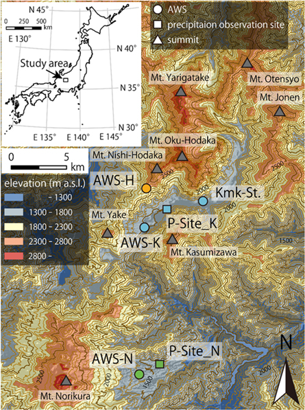
Figure 1. Map of meteorological observation sites: Kamikochi (AWS-K, blue symbols), Norikura highland (AWS-N, green symbols), and Nishi-Hodaka (AWS-H, orange symbol). Contour interval for thin lines is set as 100 m a.s.l., and that for thick lines is as 500 m a.s.l.
Download figure:
Standard image High-resolution imageThe mountainous members of the Northern Japanese Alps, Kamikochi, the Norikura highland, and Nishi-Hodaka were selected as study areas. Kamikochi is a generic term for the mountain area located in the southern part of the Northern Japanese Alps. Kamikochi is in the highland valley basin of the Azusagawa River at an elevation of 1500 m a.s.l. and is surrounded by approximately 3000 m a.s.l. high mountains in the Northern Japan Alps. In the Kamkochi region, annual cumulative snowfall over 600 mm was often observed (Suzuki 2017) from 1981 to 2012 due to the strong winter monsoon, and seasonal snow cover formed every year. The Norikura highland is 10 km south of Kamikochi. Mt. Nishi-Hodaka-dake (2909 m a.s.l.) is one of the peaks of the Hodaka Mountain Range (including Mt. Kita-Hodaka-dake, Mt. Oku-Hodaka-dake and Mt. Mae-Hodaka-dake) extending from north to south. Nishi-Hodaka is approximately 3.8 km north of Kamikochi and tops the Kamikochi Valley ridge.
2.2. Meteorological observation
Shinshu University conducted meteorological observations at an automatic weather station (AWS) in Kamikochi (AWS-K; 1490 m a.s.l.), Norikura highland (AWS-N; 1590 m a.s.l.) and Nishi-Hodaka (AWS-H; 2355 m a.s.l.) (figure 1). All sites were in open locations. The AWS-K site was selected in the forest clearing location, and in AWS-H, there are fewer trees because AWS-H is located at an elevation of the tree line; therefore, the effect of weakening wind speed is minimal in those two sites. AWS-N is in open space, but there is forest surrounding (within 5–10 m away from) the site (Nishimura et al 2018, 2019).
The instrumental specifications of the AWSs are listed in table 1. Precipitation observations were not conducted in AWS-K and AWS-N; therefore, this study used the precipitation data from the nearest observation site (Kamikochi) of the Japan Meteorological Agency as AWS-K ('P-Site_K' in figure 1), and Nrk-St. that were operated by Shinshu University ('P-Site_N' in figure 1). The authors used the observed air temperature data of Kmk-St. that was also another AWS site operated by Shinshu University (figure 1) to calculate annual meteorological statistics. Only spring season precipitation data in AWS-H were used because no observations took place during winter in this location. Precipitation, whether rain or snow was classified using the threshold air temperature of 1.7 °C (Ogawa and Nogami 1994). Observed meteorological elements (see table 2) include air temperature ( ) [°C], relative humidity (RH), wind speed (
 ) [m s−1], wind direction (WD) [degree], atmospheric pressure (P) [hPa], incoming and reflected shortwave radiation (
 and
and  ) [W m−2], incoming and upward longwave radiation (
 and
and  ) [W m−2], and snow depth (d) [m]. Every observation data was recorded in 10 min intervals. The snow depths in AWS-N and AWS-H were recorded every 60 min. The meteorological datasets were only analyzed for the snow-covered periods in 2016/17 winter, from 6 December 2016 to 4 May 2017 (AWS-K), from 24 November 2016 to 4 May 2017 (AWS-N), from 29 October 2016 to 2 July 2017 (AWS-H).
Table 1. Meteorological observation instruments used in automated weather stations in AWS-K (Kamikochi), AWS-N (Norikura) and AWS-H (Nishi-Hodaka).
| AWS-K | ||||
|---|---|---|---|---|
| observation components | instrument | accuracy | ||
| air temperature and relative humidity | air temperature | Vaisala | WXT520 | ± 0.3 °C |
| relative humidity | ± 3% (0%–90%RH) | |||
| ± 5% (90%–100%RH) | ||||
| atmospheric pressure | atmospheric pressure | Vaisala | WXT520 | ± 0.5 hPa (0 °C–30 °C) |
| ± 1 hPa (−52 °C–60 °C) | ||||
| radiation | shortwave radiation | KIPP and ZONEN | CNR 4 | ± 5% (daily sum) |
| longwave radiation | ± 10% (daily sum) | |||
| snow depth | snow depth | North one | KADEC21-SNOW | ± 1 cm |
| wind speed and wind direction | wind speed | YOUNG | Model 05103 Wind Monitor | ± 0.3 m s−1 |
| AWS-N | ||||
| observation components | instrument | accuracy | ||
| air temperature and relative humidity | air temperature | Delta OHM | HD9817T1R | ± 0.2℃ |
| relative humidity | ± 2% (10%–90%RH) | |||
| ± 2.5% (in the remaining range) | ||||
| atmospheric pressure | atmospheric pressure | Delta OHM | HD9408T | ± 0.5 hPa (20 °C) |
| radiation | shortwave radiation | KIPP & ZONEN | CNR 4 | ± 5% (daily sum) |
| longwave radiation | ± 10% (daily sum) | |||
| snow depth | snow depth | North one | KADEC21-SNOW | ± 1 cm |
| wind speed and wind direction | wind speed | YOUNG | Model 05103 Wind Monitor | ± 0.3 m s−1 |
| precipitation (Nrk-St.) | precipitation | Ota Keiki Seisakusho | 34-HP-P (Tipping Bucket Type) | ± 0.5 mm (under 20 mm) ± 3% (over 20 mm) |
| AWS-H | ||||
| observation components | instrument | accuracy | ||
| air temperature and relative humidity | air temperature | Delta OHM | HD9817T1R | ± 0.2 °C |
| relative humidity | ± 2% (10%–90%RH) | |||
| ± 2.5% (in the remaining range) | ||||
| atmospheric pressure | atmospheric pressure | Delta OHM | HD9408T | ± 0.5 hPa (20 °C) |
| radiation | shortwave radiation | KIPP & ZONEN | CNR 4 | ± 5% (daily sum) |
| longwave radiation | ± 10% (daily sum) | |||
| snow depth | snow depth | North one | KADEC21-SNOW | ± 1 cm |
| wind speed and wind direction | wind speed | YOUNG | Model 05103 Wind Monitor | ± 0.3 m s−1 |
| precipitation | precipitation | Ota Keiki Seisakusho | 34-HP-P (Tipping Bucket Type) | ± 0.5 mm (under 20 mm) ± 3% (over 20 mm) |
Table 2. Constants and variables used in this study.
| Constant | |||
|---|---|---|---|
| Symbol | Term | Value | Dimension |
| a.e., at | numeric constants | dimensionless | |
| be, bt | numeric constants | dimensionless | |
| ce, ct | numeric constants | dimensionless | |
| Cp | specific heat of air | 1005 | J kg−1 K−1 |
| cw | specific heat of water | 4.21 | kJ K−1 kg−1 |
| Lvwater | latent heat of evaporation | 2505 | kJ kg−1 |
| Lvice | latent heat of sublimation | 2838 | kJ kg−1 |
| ε | emissivity of snow surface | 0.98 | dimensionless |
| σ | Stefan-Boltzmann constant | 5.67×10⁻⁸ | W m−2 K−4 |
| κ | von Karman constant | 0.41 | dimensionless |
| ρw | water density | 1000 | kg m−3 |
| z0v | roughness length for momentum | 2.3×10⁻⁴ | m |
| Variable | |||
| Symbol | Term | Dimension | |
| CE | bulk transfer coefficient of latent heat | dimensionless | |
| CEN | neutral bulk transfer coefficient of latent heat | dimensionless | |
| CH | bulk transfer coefficient of sensible heat | dimensionless | |
| CHN | neutral bulk transfer coefficient of sensible heat | dimensionless | |
| d | snow depth | m | |
| E | latent heat flux | W m−2 | |
| H | sensible heat flux | W m−2 | |
| L | Obukhov stability length | m | |
| Lv | latent heat of water or ice | J g−1 | |
| LWin | incoming longwave radiation | W m−2 | |
| LWnet | net longwave radiation | W m−2 | |
| LWout | outgoing longwave radiation | W m−2 | |
| LWup | upward longwave radiation | W m−2 | |
| P | atmospheric pressure | Pa | |
| Pr | rainfall intensity | m s−1 | |
| Qr | rainfall energy flux | W m−2 | |
| qz | atmospheric specific humidity | g g−1 | |
| qs | specific humidity of snow surface | g g−1 | |
| q* | turbulent moisture scale | g g−1 | |
| Rnet | net radiation | W m−2 | |
| Re | roughness Reynolds number | dimensionless | |
| RH | relative humidity | dimensionless | |
| SEB | surface energy balance | W m−2 | |
| SWin | incoming shortwave radiation | W m−2 | |
| SWnet | net shortwave radiation | W m−2 | |
| SWref | reflected shortwave radiation | W m−2 | |
| Tz | air temperature | K | |
| Tr | temperature of rain drop | K | |
| Ts | surface temperature | K | |
| U | wind speed | m s−1 | |
| u* | air shear velocity | m s−1 | |
| WD | wind direction | degree | |
| zv | height of observation for wind speed | m | |
| zt | height of observation for air temperature | m | |
| ze | height of observation for relative humidity | m | |
| z0t | roughness length for temperature | m | |
| z0e | roughness length for moisture | m | |
| ρa | moist air density | g m−3 | |
| α | surface albedo | dimensionless | |
| ζ | stability parameter | dimensionless | |
| θz | atmospheric potential temperature | K | |
| θs | potential temperature of snow surface | K | |
| θ* | turbulent temperature scale | K | |
| ν | kinematic viscosity | m2 s−1 | |
| ΨM , ΨT , ΨE | stability function | dimensionless | |
2.3. Surface energy balance model
The surface energy balance (SEB) [W m−2] was determined using equation (1). The turbulent energy fluxes [W m−2] were calculated using the bulk aerodynamic method from equations (4) and (5). The rainfall energy flux ( ) [W m−2] was calculated using equation (6).


where  is the net radiation, and
  and
and  are the turbulent sensible and latent heat fluxes, respectively.
  was calculated in equations (2) and (3), where
  is the incoming shortwave radiation,
  is the reflected shortwave radiation,
  is the surface albedo,
  is the incoming longwave radiation,
  (=
(= ) is the upward longwave radiation,
  is the outgoing longwave radiation from the snow surface,
  (= 5.67×10⁻⁸ [W m−2 K−4]) is the Stefan-Boltzmann's constant, and ε (= 0.98) is the emissivity of the snow surface. In this study, surface temperature (
 ) [°C] was determined by outgoing longwave radiation using Stefan-Boltzmann's law.
  and
and  is the potential temperature of the air and the snow surface, respectively. All energy fluxes toward the surface were defined as positive.
Turbulent energy fluxes were calculated using the bulk aerodynamic method (equations (4) and (5)).  and
and  are the bulk exchange coefficients for the sensible heat and latent heat fluxes, respectively, and
  [kg m−3] is the moist air density.
  (= 1.005 [kJ K−1 kg−1]) is the atmospheric specific heat at constant pressure, and
  [J kg−1] is the latent heat of evaporation or sublimation. When
  °C, this study used Lv as the latent heat of evaporation (
 [kJ kg−1]), and when
  °C, this study used Lv as the latent heat of sublimation (
 [kJ kg−1]).
  and
and  [g kg−1] are the atmospheric and surface-specific humidity, respectively. The bulk coefficients (
 and
and  ) were calculated in a following procedure, considering the atmospheric stability by the Monin-Obukhov stability length (
 ).
).
Bulk coefficients for neutral atmospheric conditions ( and
and  ) were calculated using equations (7) and (8).


where κ (=0.41) is the von Karman constant, and 
 and
and  are the measurement height (corrected by the snow depth (d)) of wind speed, air temperature, and relative humidity (
 because of using the same sensor) at each AWS site, and
 and
and  are the roughness length for momentum, temperature, and moisture, respectively. This study was set
  [m] (Kondo and Yamazawa 1986) as a constant value.
  and
and  are calculated in equations (9) and (10), following Andreas (1987):


where  is the roughness Reynolds number,


 and
and  are the numeric constants,
  [m s−1] is the air shear velocity, and
  [m2 s−1] is the kinematic viscosity of air. Those numeric constants are given by Re, and then,
  and
and  were calculated.
This study adjusted the bulk coefficients for atmospheric stability using the Monin-Obukhov stability length, as  [m] (van den Broeke et al
2005) shown in equation (13):
[m] (van den Broeke et al
2005) shown in equation (13):


where  [K] and
  [g kg−1] are the turbulent scales of temperature and moisture, respectively. The relationships between the stability parameters
  (
( ) were determined, and the atmospheric stability was calculated as shown in (i) and (ii) (Dyer 1974). In the case of (i) or (ii), calculations were conducted using equations (16)–(18), and then, the stability functions (
 and
and  ) were calculated using
  the calculated values for each observation height (
 and
and  ).
).
- (i)
 (stable atmospheric condition)
 - (ii) (unstable atmospheric condition)


This study defined that when  is positive, the boundary layer is stable, and when
  is negative, the boundary layer is unstable, and the neutral condition is defined
  In the case of
  ∞, which means
  this study assumed no turbulence occurred in each time step.

 and
and  considering atmospheric stability were recalculated using following equations (19)–(21).


Because  is a function of
 and
and  this study conducted an iteration loop between equations (13) and (16)–(21) until
  was converged to within 0.001% of the previous value of
  Using the converged
  calculations in equations (16)–(18) were conducted. The values of

 and
and  were calculated using equations (4), (5), (22), and (23).


Rainfall energy flux is the sensible heat supplied by raindrops.  was calculated using equation (6).
  [m s−1] is the rainfall intensity,
  (=1000 [kg m−3]) is the density of the water,
  (= 4.21 [kJ K−1 kg−1]) is the specific heat capacity of the water, and
  is the temperature of a rain drop, which is considered equal to
  in this study. This study neglected the subsurface energy flux because its contribution to the surface energy balance is small (e.g. Andreassen et al
2008, Sicart et al
2008). In addition, this assumption is applied widely during the ablation period, because the entire snowpack is assumed to be 0 °C in that period. Therefore, this study discussed the results of surface energy balance analysis during the ablation period (in table 5 and figure 4).
in this study. This study neglected the subsurface energy flux because its contribution to the surface energy balance is small (e.g. Andreassen et al
2008, Sicart et al
2008). In addition, this assumption is applied widely during the ablation period, because the entire snowpack is assumed to be 0 °C in that period. Therefore, this study discussed the results of surface energy balance analysis during the ablation period (in table 5 and figure 4).
3. Result
3.1. Meteorological observation data
The annual mean air temperature and the annual amount of precipitation in Kamikochi, Norikura, and Nishi-Hodaka are shown in table 3. However, annual precipitation was not calculated because all year precipitation observations in AWS-H were not conducted. The annual mean air temperatures in Kamikochi, Norikura, and Nishi-Hodaka were 5.8 °C, 5.5 °C, and 1.3 °C, respectively. The annual ranges of air temperature in Kamikochi, Norikura, and Nishi-Hodaka were 25.7 °C, 24.7 °C, and 26.0 °C, respectively. The annual cumulative precipitation in Kamikochi and Norikura were 2692 mm and 1946 mm, respectively.
Table 3. Annual mean air temperature [°C], the annual range of air temperature [°C], and their standard deviation (SD) in Kamikochi, Norikura, and Nishi-Hodaka, and annual cumulative precipitation [mm] and its standard deviation in Kamikochi and Norikura.
| Air temperature [°C] | Precipitation [mm] | ||||||
|---|---|---|---|---|---|---|---|
| region | Kamikochi | Norikura | Nishi-Hodaka | Kamikochi | Norikura | Nishi-Hodaka | |
| period | 2010–2018 | 2003–2018 | 2010–2018 | 2007–2018 | 2007–2018 | ||
| annual mean | 5.8 | 5.5 | 1.3 | Annual cumulative | 2692 | 1946 | no data |
| SD | 0.7 | 0.5 | 0.6 | SD | 283 | 278 | no data |
| annual range | 25.2 | 24.7 | 25.8 | — | — | — | |
| SD | 1.1 | 1.2 | 1.4 | — | — | — | |
Meteorological observation data during the snow-covered period of 2016/17 in AWS-K, AWS-N, and AWS-H are shown in figure 2. The air temperature difference between AWS-K and AWS-N was small, and a similar fluctuation of air temperature in AWS-K and AWS-N was observed. The air temperature in AWS-H was lower than that in the other two sites, reflecting a difference in the elevation of the AWS location. The positive air temperature was observed after early April in AWS-K and AWS-N, and after late April AWS-H. No noticeable differences in specific humidity were found. However, the specific humidity in the AWS-H was slightly higher than that in the other both sites. The fluctuation in specific humidity at all sites was similar. The wind speed at AWS-H was higher than that in the other two sites, and the wind speed in AWS-N was slightly lower than that in AWS-K. The mean wind speed during the snow-covered period in AWS-H was over 2.5 times higher than that in the other two sites. The snow depth in AWS-H was much larger than that in the other two sites. The maximum snow depths in 2016/17 in AWS-H, AWS-K, and AWS-N were 676 cm, 165 cm and 159 cm, respectively. Decreasing snow depth was observed in all sites after early April.
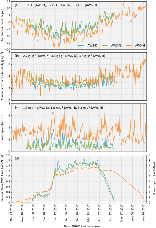
Figure 2. Result of meteorological observation in AWS-K (Kamikochi), AWS-N (Norikura), and AWS-H (Nishi-Hodaka); daily mean (a) air temperature [°C], (b) atmospheric specific humidity [g kg−1], (c) wind speed [m s−1] and (d) snow depth [cm] in snow-covered period. Figures in each graph are averaged values for the snow-covered period.
Download figure:
Standard image High-resolution image3.2. Surface energy balance analysis
All locations showed distinct surface energy balance properties, those were (1) net shortwave radiation controlled SEB variation and (2) an energy loss due to negative latent heat flux. The analysis of the surface energy balance during the ablation period is shown in table 4, and the energy flux in figure 3. The figures showing each energy balance component's contribution ratio in the text and table 4 were calculated by dividing an energy flux (e.g., net shortwave radiation, net longwave radiation) by the total energy flux (SEB). Net shortwave radiation is the most dominant energy source at all sites (over 100%), and the second major energy flux was the sensible heat flux. Net longwave radiation was the largest source of energy loss at all sites. Latent heat flux was the second source of energy loss at AWS-K and AWS-N, but it was the third largest source of positive energy flux at AWS-H. Rainfall energy flux hardly contributed to the snow ablation at all sites. This resulted in a radiation component that controlled the surface energy balance variation and snow ablation process.
Table 4. Result of energy balance analysis for the ablation period in AWS-K (Kamikochi), AWS-N (Norikura), and AWS-H (Nishi-Hodaka). Respective energy flux for monthly mean and average of snow-covered periods are shown on the left. The values in parentheses show the proportion of SEB (QM ). Figures in the month with ' * ' showing those figures do not meet statistical significance due to a data shortage.
| SEB | Net shortwave radiation | Net longwave radiation | Sensible heat flux | Latent heat flux | Rainfall energy flux | |||||||||
|---|---|---|---|---|---|---|---|---|---|---|---|---|---|---|
| W m−2 | (%) | W m−2 | (%) | W m−2 | (%) | W m−2 | (%) | W m−2 | (%) | W m−2 | (%) | |||
| AWS-K | Feb. | 8.5 | (100.0) | 28.3 | (331.2) | −20.3 | (−237.4) | 7.7 | (89.9) | −6.4 | (−75.2) | 0.2 | (2.3) | |
| Mar. | 16.0 | (100.0) | 43.0 | (268.6) | −26.1 | (−163.1) | 6.0 | (37.5) | −8.1 | (−50.4) | 0.0 | (0.0) | ||
| Apr. | 76.8 | (100.0) | 85.1 | (110.8) | −19.9 | (−25.9) | 13.6 | (17.7) | −4.7 | (−6.1) | 2.2 | (2.9) | ||
| May | * | 175.9 | (100.0) | 170.8 | (97.1) | −12.1 | (−6.9) | 17.3 | (9.9) | −0.3 | (−0.2) | 0.1 | (0.1) | |
| June | — | — | — | — | — | — | — | — | — | — | — | — | ||
| July | — | — | — | — | — | — | — | — | — | — | — | — | ||
| ALL | 28.0 | (100.0) | 43.4 | (155.3) | −19.7 | (−70.6) | 8.6 | (30.8) | −5.6 | (−19.9) | 0.5 | (1.9) | ||
| AWS-N | Feb. | 17.6 | (100.0) | 28.7 | (162.8) | −15.3 | (−86.9) | 5.4 | (30.9) | −1.3 | (−7.6) | 0.0 | (0.0) | |
| Mar. | 37.7 | (100.0) | 58.9 | (156.2) | −24.1 | (−63.8) | 4.8 | (12.7) | −3.8 | (−9.9) | 0.0 | (0.0) | ||
| Apr. | 95.7 | (100.0) | 100.5 | (104.9) | −14.5 | (−15.1) | 8.3 | (8.6) | 0.0 | (0.0) | 0.9 | (0.9) | ||
| May | * | 147.7 | (100.0) | 147.4 | (99.9) | −13.4 | (−9.1) | 10.8 | (7.3) | 2.2 | (1.5) | 0.6 | (0.4) | |
| June | — | — | — | — | — | — | — | — | — | — | — | — | ||
| July | — | — | — | — | — | — | — | — | — | — | — | — | ||
| ALL | 36.9 | (100.0) | 48.4 | (131.3) | −17.2 | (−46.6) | 5.9 | (15.9) | −1.2 | (−3.3) | 0.2 | (0.6) | ||
| AWS-H | Feb. | 19.4 | (100.0) | 42.5 | (218.7) | −25.3 | (−130.0) | 1.2 | (6.2) | 0.1 | (0.4) | No Data | No Data | |
| Mar. | 26.7 | (100.0) | 43.3 | (162.0) | −19.2 | (−71.7) | 1.9 | (7.1) | −0.9 | (−3.4) | No Data | No Data | ||
| Apr. | 72.4 | (100.0) | 96.2 | (132.8) | −30.1 | (−41.6) | 6.1 | (8.5) | −2.2 | (−3.1) | 1.0 | (1.3) | ||
| May | 192.4 | (100.0) | 177.7 | (92.3) | −11.5 | (−6.0) | 19.7 | (10.2) | 5.8 | (3.0) | 0.8 | (0.4) | ||
| June | 225.5 | (100.0) | 181.7 | (80.6) | −1.5 | (−0.6) | 25.1 | (11.1) | 18.4 | (8.2) | 1.7 | (0.8) | ||
| July | * | 311.8 | (100.0) | 23.0 | (7.4) | 65.2 | (20.9) | 77.1 | (24.7) | 98.3 | (31.5) | 48.1 | (15.4) | |
| ALL | 80.8 | (100.0) | 87.7 | (108.6) | −18.4 | (−22.8) | 8.0 | (9.9) | 2.2 | (2.7) | 0.8 | (1.0) | ||
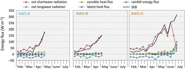
Figure 3. Result of energy balance analysis in AWS-K (Kamikochi), AWS-N (Norikura), and AWS-H (Nishi-Hodaka). A month is divided into three parts, which are the first ten days of the month (1st to 10th), followed by the next ten days (11th to 20th), and finally the remainder of the month (21st to the end of the month), and variation of each energy component shown. Data plot symbol represented by a diamond does not meet statistical significance due to a data shortage.
Download figure:
Standard image High-resolution imageThe trends observed at each site can be summarized as follows: The surface energy balance was controlled by net shortwave radiation in AWS-K, which is 155.3% against SEB. The other significant energy flux was the sensible heat flux (30.8%). The net longwave radiation and latent heat flux were the energy sink and cooled the snow surface at −70.6% and −19.9%, respectively. The energy loss due to longwave radiation emission and latent heat flux in AWS-K was more extensive than that of the other two sites. The rainfall energy flux was a small source of energy (1.9%).
The surface energy balance property in AWS-N was similar to that in AWS-K. The largest energy source was net shortwave radiation (131.3%), and the second was a sensible heat flux (15.9%). In contrast, the greatest energy sink was net longwave radiation (−46.6%), followed by the latent heat flux (−3.3%). The rainfall energy flux was also a small positive energy source (0.6%).
The surface energy balance property at AWS-H was also similar to those in AWS-K and AWS-N. However, the amount of net shortwave radiation (108.6%) and the sensible heat flux (9.9%) were larger than those of AWS-K and AWS-N. Latent heat flux was negative in March and April (slightly positive in February), and then it turned to positive between May and July.
4. Discussion
4.1. Surface energy balance in Northern Japanese Alps region
We evaluated the surface energy balance properties for the Northern Japanese Alps: (1) net radiation that controlled the surface energy balance variation, and (2) negative latent heat flux (sublimation) in the mid-winter season. Net radiation contributed significantly (over 80%) to snow ablation in the Northern Japanese Alps, due to high net shortwave radiation (over 100%). The ablation-dominating shortwave radiation (e.g. Greuell and Smeets 2001) has been reported on by many previous studies. Therefore, a special snow ablation mechanism could not be recognized in the Northern Japanese Alps.
The surface energy balance properties of (1) and (2) described above were similar to continental climate regions (Willis et al 2002), suggesting that the snow cover was ablates in relatively dry atmospheric conditions during the winter season. Shortwave radiation increases due to less cloud formation (Abermann et al 2019) and energy sink in sublimation from snowpack when it is dry (Sicart et al 2005). The Japanese climate is considered maritime; therefore, there are reports on surface energy balance analyses for maritime climates (e.g. Matsumoto et al 2010). However, the surface energy balance property in continental climate region noted in Sicart et al (2005) was also confirmed in this study region in the mid-winter season.
This study reviewed previous reports and classified the surface energy balance according to continental or maritime climate (partly referring to Willis et al (2002) and Giesen et al (2008)). The results of the review are shown in table 5 and figure 4. The surface energy balance analysis data of this study listed in table 5 are only for the ablation period. Radiation elements are generally dominant (e.g. Sicart et al 2005) in continental climate region, and turbulent energy flux, in contrast, dominates the surface energy balance (e.g. Gillett and Cullen 2011). Data in this study listed in table 5 are similar to the surface energy balance property one expects of a continental climate region. Accumulated and ablated snow cover in relatively dry atmospheric, continental climate, conditions in this study are a new description, because the Japanese seasonal snow cover accumulation and ablation was generally thought to be governed by the maritime climate.
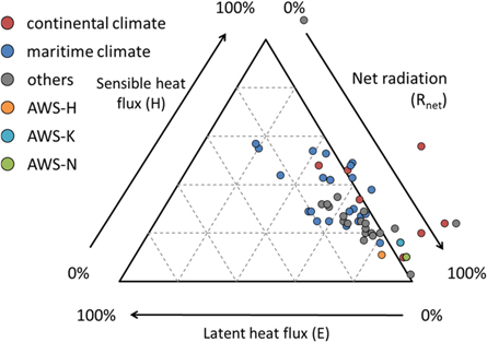
Figure 4. Triangular diagram showing three energy components, net radiation, sensible heat flux and latent heat flux, of the previous study in table 5.
Download figure:
Standard image High-resolution imageTable 5. Data used from the previous study in figure 4: study location, latitude, altitude, climate classification, observation period, and the surface energy balance.
| Location | Observation Period | Surface Energy Flux (%) | References | |||||||||||
|---|---|---|---|---|---|---|---|---|---|---|---|---|---|---|
| Site | Country | Latitude | Altitude (m) | Climate | Rnet | H | E | |||||||
| Kamikochi | Japan | 36° N | 1490 | Apr. | 2017 | — | May | 2017 | 85 | 16 | −4 | this study | ||
| Norikura | Japan | 36° N | 1590 | Feb. | 2017 | — | May | 2017 | 92 | 10 | −3 | this study | ||
| Nishi-Hodaka | Japan | 36° N | 2355 | Mar. | 2017 | — | Jul. | 2017 | 83 | 11 | 5 | this study | ||
| Peyto Glacier, Alberta | Canada | 51° N | 2500 | Continental | Jun. | 1988 | — | Jul. | 1988 | 51 | 42 | 7 | Munro (1990) | |
| Peyto Glacier, Alberta | Canada | 51° N | 2300 | Continental | Jun. | 1988 | — | Jul. | 1988 | 65 | 34 | 1 | Munro (1990) | |
| Peyto Glacier, Alberta | Canada | 51° N | 2510 | Continental | Jul. | 1970 | 44 | 48 | 8 | Föhn (1973) | ||||
| Hintereisferner | Austria | 46° N | 2500 | Continental | Jul. | 1986 | 91 | 10 | −2 | van de Wal et al (1992) | ||||
| Hintereisferner | Austria | 46° N | 2630 | Continental | Jul. | 1989 | 93 | 20 | −13 | van de Wal et al (1992) | ||||
| Niwot Ridge, CO | USA | 40° N | 3517 | Continental | Apr. | 1994 | — | Jun. | 1994 | 75 | 56 | −31 | Cline (1997) | |
| Valee Blanche | France | 45° N | 3550 | Continental | Jul. | 1968 | 99 | 24 | −23 | De la Casiniere (1974) | ||||
| St Sorline Glacier | France | 2712 | Continental | Aug. | — | Sep. | 1969 | and 1970 | 61 | 46 | −1 | Martin (1975) | ||
| Storglaciären | Sweden | 68° N | 1370 | Maritime | Jul. | 1994 | — | Aug. | 1994 | 66 | 30 | 5 | Hock and Holmgren (1996) | |
Qamanârss p sermia p sermia | Greenland | 64° N | 790 | Maritime | Jun. | 1980 | — | Aug. | 1986 | 67 | 38 | −5 | Braithwaite and Olesen (1990) | |
| Ecology Glacier, King George Island | Antarctica | 62° S | 100 | Maritime | Dec. | 1990 | — | Jan. | 1991 | 64 | 29 | 7 | Bintanja (1995) | |
| Worthington Glacier, AK | USA | 61° N | Maritime | Jul. | 1967 | — | Aug. | 1967 | 51 | 29 | 21 | Streten and Wendler (1968) | ||
| Worthington Glacier | Alaska | 61° N | 820 | Maritime | Jul. | 1967 | — | Aug. | 1967 | 51 | 29 | 20 | Streten and Wendler (1968) | |
| Qamanârssp sermia | Greenland | 61° N | 880 | Maritime | Jun. | 1979 | — | Aug. | 1983 | 70 | 28 | 2 | Braithwaite and Olesen (1990) | |
| Lemon Creek Glacier | Alaska | 58° N | 1200 | Maritime | Aug. | 1968 | — | Aug. | 1968 | 48 | 43 | 9 | Wendler and Streten (1969) | |
| Kryoto Glacier | Russia | 55° N | 810 | Maritime | Aug. | 2000 | — | Sep. | 2000 | 33 | 44 | 23 | Konya et al (2004) | |
| Hodges Glacier | South Georgia | 54° S | 375 | Maritime | Nov. | 1973 | — | Apr. | 1974 | 55 | 48 | −3 | Hogg et al (1982) | |
| Glacier Lengua | Chile | 53° S | 450 | Maritime | Feb. | 2000 | — | Apr. | 2000 | 35 | 54 | 7 | Schneider et al (2007) | |
| Tyndall Glacier | Chile | 51° S | 700 | Maritime | Dec. | 1993 | 51 | 42 | 7 | Takeuchi et al (1995a, 1995b) | ||||
| Moreno Glacier | Chile | 50° S | 330 | Maritime | Nov. | 1993 | 54 | 49 | −4 | Takeuchi et al (1995a, 1995b) | ||||
| Ampere Glacier | Kerguelen Island | 49° S | Maritime | Jan. | 1972 | — | Mar. | 1972 | 58 | 25 | 16 | Poggi (1977) | ||
| Soler Glacier | Chile | 46° S | 378 | Maritime | Nov. | 1985 | 57 | 43 | −1 | Fukami and Naruse (1987) | ||||
| Brewster Glacier | New Zealand | 44° S | 1770 | Maritime | Dec. | 2007 | — | Mar. | 2008 | 52 | 25 | 20 | Gillett and Cullen (2011) | |
| Brewster Glacier | New Zealand | 44° S | 1760 | Maritime | Oct. | 2010 | — | Sep. | 2012 | 64 | 23 | 11 | Cullen and Conway (2015) | |
| Brewster Glacier | New Zealand | 44° S | 1760 | Maritime | Oct. | 2010 | — | Sep. | 2012 | 37 | 53 | 3 | Conway and Cullen (2016) | |
| Franz Josef Glacier | New Zealand | 43° S | Maritime | Feb. | 1990 | 21 | 55 | 25 | Ishikawa et al (1992) | |||||
| Mount Cook National Park | New Zealand | 43° S | Maritime | Oct. | 1995 | — | Nov. | 1995 | 63 | 27 | 4 | Neale and Fitzharris (1997) | ||
| Temple Basin | New Zealand | 42° S | 1450 | Maritime | Oct. | 1982 | — | Nov. | 1982 | 16 | 57 | 25 | Moore and Owens (1984) | |
| Niigata | Japan | 37° N | 360 | Maritime | Dec. | 2007 | — | Apr. | 2008 | 80 | 16 | 3 | Matsumoto et al (2010) | |
| Blue Glacier, WA | USA | Maritime | Jul. | 1958 | — | Aug. | 1958 | 69 | 25 | 6 | La Chapelle (1959) | |||
| Location | Observation Period | Surface Energy Flux (%) | Reference | |||||||||||
| Site | Country | Latitude | Altitude (m) | Climate | Rnet | H | E | |||||||
| Berkner Island | Antarctica | 79° S | 886 | Others | Feb. | 1995 | — | Dec. | 1997 | −91 | 108 | −17 | Reijmer et al (1999) | |
| McCall Glacier | Alaska | 69° N | 1715 | Others | Jun. | 2004 | — | Aug. | 2004 | 74 | 25 | 5 | Klok et al (2005) | |
| Storglaciären | Sweden | 67° N | 1370 | Others | Jul. | 2000 | — | Sep. | 2000 | 55 | 32 | 13 | Sicart et al (2008) | |
| Vestari Hagafellsjökull | Iceland | 64° N | 500 | Others | Jun. | 2001 | — | Aug. | 2007 | 63 | 27 | 10 | Matthews et al (2015) | |
| Vestari Hagafellsjökull | Iceland | 64° N | 1100 | Others | Jun. | 2001 | — | Aug. | 2009 | 74 | 20 | 6 | Matthews et al (2015) | |
| West Gulkana Glacier | Alaska | 63° N | 1520 | Others | Jun. | 1986 | — | Jul. | 1986 | 57 | 35 | 8 | Brazel et al (1992) | |
| Storbreen | Norway | 62° N | 1600 | Others | Jul. | 1955 | — | Sep. | 1955 | 56 | 31 | 13 | Liestøl (1967) | |
| Storbreen | Norway | 62° N | 1570 | Others | Sep. | 2001 | — | Sep. | 2006 | 76 | 17 | 8 | Giesen et al (2009) | |
| Nordbogletscher | Greenland | 61° N | 880 | Others | Jun. | 1979 | — | Aug. | 1983 | 71 | 29 | 2 | Braithwaite and Olesen (1990) | |
| Omnsbreen | Norway | 60° N | 1540 | Others | Jun. | 1968 | — | Sep. | 1969 | 52 | 32 | 15 | Messel (1971) | |
| Midtdalsbreen | Norway | 60° N | 1450 | Others | Oct. | 2000 | — | Sep. | 2006 | 67 | 24 | 10 | Giesen et al (2008) | |
| Midtdalsbreen | Norway | 60° N | 1450 | Others | Sep. | 2001 | — | Sep. | 2006 | 66 | 25 | 11 | Giesen et al (2009) | |
| Pasterze | Austria | 47° N | 2205 | Others | Jun. | 1994 | — | Aug. | 1994 | 77 | 20 | 4 | Greuell and Smeets (2001) | |
| Pasterze | Austria | 47° N | 2310 | Others | Jun. | 1994 | — | Aug. | 1994 | 73 | 22 | 5 | Greuell and Smeets (2001) | |
| Pasterze | Austria | 47° N | 2420 | Others | Jun. | 1994 | — | Aug. | 1994 | 72 | 24 | 4 | Greuell and Smeets (2001) | |
| Pasterze | Austria | 47° N | 2945 | Others | Jun. | 1994 | — | Aug. | 1994 | 77 | 19 | 4 | Greuell and Smeets (2001) | |
| Pasterze | Austria | 47° N | 3225 | Others | Jun. | 1994 | — | Aug. | 1994 | 79 | 20 | 1 | Greuell and Smeets (2001) | |
| St Sorlin | France | 45° N | 2760 | Others | Jul. | 2006 | — | Aug. | 2006 | 84 | 22 | −5 | Sicart et al (2008) | |
| Indian Himalaya | India | 32° N | 3050 | Others | Jan. | 2005 | — | Apr. | 2005 | 98 | 3 | −1 | Datt et al (2008) | |
| Zongo Glacier | Bolivia | 16° S | 5050 | Others | Nov. | 1999 | — | Dec. | 1999 | 103 | 24 | −27 | Sicart et al (2008) | |
The high humidity air mass is advected to Japan caused by the East Asian monsoon, and steep elevation gradients in the region from the coast of the Sea of Japan to the Japanese Alps formed the dry atmospheric conditions (see figure 5). A warm and humid air mass from the Eurasian continent is supplied to the coastal area of the Sea of Japan (Magono et al 1966) due to three factors:
- (1)Siberian anticyclone formation on the East Eurasian continent in winter
- (2)Cyclones in the Pacific Ocean
- (3)

Figure 5. Mechanism that forms the specific atmospheric condition and the surface energy balance property in the Northern Japanese Alps.
Download figure:
Standard image High-resolution image
This mechanism is known as the representative Japanese winter monsoon. It yields heavy snowfall in the coastal areas because the humid air mass originating from the winter monsoon is forced to lift over the Northern Japanese Alps (Estoque and Ninomiya 1976). Precipitation rarely occurs in the island area due to typical meteorological conditions. There is an amount of precipitation gradient between the windward (north west) area and the lee side (south east) area of the Northern Japanese Alps. A precipitation gradient similar to that in the Northern Japanese Alps was reported by Viale et al (2019). It showed that an East-West precipitation gradient in Patagonia, Chile made a distinction in climate between the windward area and the lee side area in the Andes Mountains. Moreover, Ikeda et al (2009) also showed that the climate condition in the lee side of the Northern Japanese Alps is dry, it is based on the snowpack observation of physical properties. The specificity of our surface energy balance analysis was established in addition to Ikeda et al (2009), the mechanism of snowfall in Japan, and the environment of seasonal snow cover.
4.2. Surface energy balance properties in Kamikochi, Norikura highland and Nishi-Hodaka
The topographic condition, surrounding vegetation, and elevation difference are specific surface energy balance properties in AWS-K, AWS-N, and AWS-H. AWS-K is located at the bottom of a valley terrain; a cold air pool is typically formed. When a cold air pool is formed, a stable stratification in the boundary layer and radiation cooling occurs, and sublimation of the snowpack further cooled the snow surface further. Snowpack cooling frequently occurs in the AWS-K. The surface energy balance property in AWS-N resembled that of in AWS-K. There is no distinct difference in air temperature and atmospheric specific humidity with AWS-K and AWS-N. However, the turbulent energy flux in AWS-N was smaller than that of in AWS-K. Surrounding vegetation allowed the wind speed to decrease, resulting in the increased formation of a stable boundary layer and restraining turbulence.
The differences in air temperature due to the atmospheric pressure and the amount of snowfall among in AWS-K, AWS-N, and AWS-H make the characteristic of surface energy balance in AWS-H. The major meteorological differences among AWS-K and AWS-N against AWS-H are as follows: in AWS-H, (1) a period in which the daily mean air temperature turns to be positive is later and (2) the snow-covered duration is longer than those in the AWS-K and AWS-N. Thus, significant snow ablation in AWS-H begins later and stronger snow melt occurred in the late ablation period than those in the other two sites. In addition, incoming shortwave radiation, air temperature, and atmospheric humidity increase with time. This consideration, therefore, reveals the characteristics of AWS-H, that is, net shortwave radiation and turbulent heat flux large in the late ablation period, and rapid snow ablation is occurred, as well as the difference in the surface energy balance properties among the three AWS sites located in the same climate region.
5. Conclusion
We discussed the surface energy properties of the Northern Japanese Alps, Kamikochi, Norikura highland, and Nishi-Hodaka. The surface energy balance property in this region was similar to that in the continental climate region because of the Japanese specific climate (winter monsoon) and topographic (steep elevation gradient) conditions of the Japanese Alps. The representative Japanese winter monsoon supplies warm and humid air masses to the Japanese Alps, resulting in heavy snowfall in the coastal areas. This forms a climate contrast between the windward and leeward areas of the Northern Japanese Alps. Therefore, we conclude that the seasonal snow cover on the lee side of the Northern Japanese Alps was formed under relatively dry atmospheric conditions. This is a new finding, considered with a surface energy balance analysis. Some areas in the Japanese Alps are dry, while the Japanese climate is usually regarded as a maritime climate.
There were some area-specific surface energy balance properties in Kamikochi, Norikura highland and Nishi-Hodaka. These properties were affected by the topographic conditions in Kamikochi, surrounding vegetation in the Norikura highland, and low air temperature conditions in Nishi-Hodaka due to the high elevation. The AWS sites are only approximately 10 km apart; however, a unique surface energy balance property was found for each site.
Acknowledgments
The outcomes of this study were obtained when the first author was attending a graduate program at Shinshu University, and all data used in this study are attributed to Shinshu University. We are grateful to everyone who supported this study. In addition, a part of this work (primarity data analysis) was conducted using resources from the Arctic Challenge for Sustainability II (ArCS II), Program Grant Number JPMXD1420318865. The Nishiho Mountain Lodge is thanked for their generous cooperation with our field survey. Meteorological data obtained by Shinshu University are publicly available in http://ims.shinshu-u.ac.jp/ (Japanese only). Some precipitation data observed by the Japan Meteorological Agency used in this research are from https://www.jma.go.jp/jma/indexe.html.
Data availability statement
The data generated and/or analysed during the current study are not publicly available for legal/ethical reasons but are available from the corresponding author on reasonable request.