Abstract
We show theoretically how a sequence of spatial light modulators (SLMs) can be used to compensate polarisation and phase errors introduced by a spatially variant homogeneous waveplate with any polarisation eigenmode and arbitrary retardance distribution. The resultant compensation is applicable to all pure input polarisation states. The properties of such a system are easily described using Jones calculus in terms of the retardance distribution on each SLM. However, it is not straightforward to determine from the Jones matrices the arrangements nor the settings of each SLM required to implement an arbitrary spatially variant retarder. In order to address this problem, analytic solutions for the required SLM settings are obtained through the construction of a geometrical model on the Poincaré sphere. These solutions are validated against numerical models. These models can be used, for example, to control a multi-pass SLM system acting as the correction device in an efficient vectorial adaptive optics system.
Export citation and abstract BibTeX RIS

Original content from this work may be used under the terms of the Creative Commons Attribution 4.0 license. Any further distribution of this work must maintain attribution to the author(s) and the title of the work, journal citation and DOI.
1. Introduction
A range of applications in classical and quantum optics require the control of the spatially variant vectorial state of light—encompassing both polarisation and phase [1–3]. These applications include focusing through high numerical aperture lenses; using optical elements like Q plates [4, 5], metasurfaces and graded-index optics [6, 7]; plasmonic or waveguiding structures [8, 9]; and laser machining [10].
Some emerging applications require compensation of spatially variant perturbations of the vectorial state (vectorial aberrations) when light propagates through an optical system [7, 11–14]. This can occur, for example, in imaging systems like microscopes or lithography systems whose performance is sensitive to the polarisation state of the light. In addition to suffering from the effects of phase aberrations, which vary from specimen to specimen, the performance of these microscopes also degrades when the light deviates from the ideal polarisation state. This includes super-resolution methods, such as stimulated emission depletion microscopy and structured illumination microscopy [15–17]. By their nature, these systems require adaptive compensation of phase and polarisation errors. Vectorial aberrations can also be introduced when focussing through birefringent crystals, through stressed optical elements or due to dielectric coatings [7, 18, 19]. Adaptive optical elements could be used to correct the vectorial aberrations introduced in such systems. While adaptive optics has been widely used for phase correction, its use for polarisation control is more challenging, due to more degrees of freedom being required to control the vectorial field. This would require a complex optical system with multiple adaptive elements. Despite this complexity, many systems have already been implemented that use multiple adaptive elements [20–22].
Control of both polarisation and phase requires control of at least three independent variables, as there are three degrees of freedom in the description of the vectorial state (for example, this is clear when one considers the two degrees representing the coordinates of a point on the Poincare sphere (PS) in addition to one for the phase). However, it was recently shown that conversion between two arbitrary vectorial states required a sequence of four—rather than three—passes through parallel aligned liquid crystal spatial light modulators (SLMs). Note that multiple passes could be implemented by different areas of the single SLM, so fewer than four devices could be used in practice. Four passes were necessary, as these commonly used SLMs are in effect fixed-axis, variable linear retarders; the fixed axes lead to degeneracies in the operation of the SLMs when input states are aligned with the axes of the retarders [23]. This previous work addressed the limited case of conversion between a pair of vectorial states, but not the more general problem of compensating the polarisation errors induced by a medium for all possible input states on the PS.
In this paper, we show how full vectorial compensation for all input states can be achieved using appropriate combinations of four SLM passes (or three SLM passes in combination with polarisation insensitive device, such as a deformable mirror (DM)). The combination of polarisation and phase perturbations introduced by an optical system can be described by an equivalent Jones matrix. Similarly, the correction required to compensate for such a system should be described by a 'conjugate' Jones matrix. If the Jones matrix of the system were known, then it should be possible to set the multi-pass SLM system to compensate the perturbation by mimicking the conjugate retarder. We provide a method and analytic expressions for determining the settings of the SLMs in terms of the properties of the desired retarder.
2. Background
In this section, we derive the Jones matrix description of a series of SLM passes and compare this to the Jones matrix for a generalised elliptical retarder. We then explain how comparisons based upon the eigenmodes of the two systems can be used to build the geometric models to determine the SLM settings.
2.1. Jones matrices of SLM combinations
As a starting point, we consider a four pass SLM system that was previously shown to be sufficient to convert between two fixed arbitrary vectorial states [23]. Alternatively, the same effect could be achieved using a sequence of three SLMs and a DM. The sequence is shown in figure 1. For brevity, we will refer to these devices just as 'SLMs'. The axes of the SLMs are oriented in sequence at 0°, 45° and 0°. All of the SLMs are assumed to be in planes optically conjugate to the system pupil, so that their effects can be modelled in terms of the 'Jones pupil', onto which all spatially variant retardance effects in the system can be mapped. The Jones matrix  of the combination represented in this pupil is given by the product of the four Jones matrices of each of the individual elements.

Figure 1. Schematic of the multiple SLM and DM system. The modulation axis (slow axis orientation) of each SLM is set at the indicated angle. For notational simplicity, we model these devices as closely spaced transmissive elements, although they are reflective in most practical cases and connected by imaging relay optics. In practice, the multiple SLM passes by be implemented as passes through separate regions of the same SLM.
Download figure:
Standard image High-resolution imageNote that all retardances and related variables used here are functions of position in the Jones pupil. For notational simplicity, this spatial variation is not written explicitly

The individual Jones matrices are presented here, where the offset phase corresponding to the fixed phase shift at the non-modulating axis has been neglected
 ,
,  , and
, and  are the retardances of SLM1, SLM2 and SLM3, respectively.
  is the phase introduced by the DM. As the DM is polarisation insensitive, the Jones matrix is simply defined here as a complex scalar variable multiplied by the identity matrix. We note that this Jones matrix strictly speaking describes a transmissive phase element, rather than a reflective element, but we choose this representation for mathematical clarity. As the retardance of these devices is spatially variable, each of the phase values is a function of the spatial coordinates across the device, although this dependence is omitted from the expressions for the sake of clarity.
2.2. Jones matrix of general elliptical retarder
The Jones matrix  of a generalised elliptical retarder can be expressed as
where  is the ellipse orientation,
  is the retardance, and
  is the parameter that determines the ellipticity of the eigenstate. Note that this retardance
  needs to be equal to the negative of the retardance of the retarder for which we need to compensate, so that the Jones matrix
  conjugate to the perturbation retarder. In order for the SLM system to perfectly mimic the elliptical retarder, it is necessary for the Jones matrices
  and
and  to be equal. It is a non-trivial task to determine the required retardances directly from these expressions. Hence, we have developed a geometrical approach involving transitions on the PS in order to obtain the necessary SLM settings.
2.3. Eigenvalues and equivalent retardance for SLM combinations
For the two retarders to be equivalent, their eigensystems must also be equivalent. Hence, the task can be reduced to the problem of setting the SLM retardances so that the eigenvectors and eigenvalues in each case are equal. The eigenvectors are equivalent to the waveplate axes and the retardance is given by the difference between the phases of the eigenvalues.
In order to determine the eigenvalues  and
and  , let us define the Jones matrix of the three SLMs as

The dynamic phase offset  is given by the argument of the determinant of the Jones matrix, which is readily obtained as
We adjust equation (4) by removing this phase factor to give

where
has zero dynamic phase. The eigenvectors and eigenvalues of  can thus be found as the solution to the equation
or alternatively
Solving this quadratic equation gives the two eigenvalues as

with
The retardance  of the equivalent retarder described by
  is given by
This provides a relationship between the retardance of the SLM combination and the settings of the individual SLMs. However further conditions must be placed on the eigenvectors for the SLM combination to be equivalent to the chosen retarder.
2.4. Eigensystems for SLM combinations
There is insufficient information in the expressions shown above to make the Jones matrix of the three-SLM system equivalent to a chosen arbitrary retarder. However, the necessary relationships can be obtained through geometrical considerations concerning the eigenvectors.
We need to note that if the input to the system is an eigenmode, then the output will be the same eigenmode. When an input polarisation state is transformed by a sequence of retarders, the state will evolve along a path on the PS. If the path is closed—i.e. when the output state is the same as the input state—then the input state must be aligned with an eigenvector of the system. For our system to be equivalent to the chosen retarder, we must therefore ensure that the sequence of SLMs causes a closed path to be traced out on the PS that starts from and returns to the point represented by the eigenvector of the retarder. As the two eigenvectors of a retarder are diametrically opposed on the PS, by symmetry, a sequence of SLMs that achieves a closed path for one eigenvector must also achieve the same for the other eigenvector.
Following progression through the sequence of SLMs, the eigenmode acquires a phase shift, which is given by the argument of the corresponding eigenvalue. These phase shifts will generally not be the same for the two eigenmodes, but the difference between the phases is equivalent to the retardance of the system.
3. Linear retarders implemented through the multiple SLM system
3.1. Linear retarders—eigenvectors
We illustrate this principle using the three-SLM system to act as a linear retarder of retardance  , whose extraordinary axis is oriented at an angle
  . The primary eigenvector of this retarder is represented by a point on the equator (
 plane) of the PS at a longitude of
  , shown at point A.
Figure 2 shows how a closed path ABCA can be constructed using three arcs: AB is due to the action of the first SLM, whose primary eigenvector is aligned with the  axis; BC is due to the second SLM with eigenvector along the
  axis; CA is from the third SLM with eigenvector along the
  axis. Note that point C is the reflection of point B in the
  plane. The angles subtended by the arcs at their respective eigenmode axes are equal to the retardances of the SLMs, respectively
  ,
,  , and
, and  . The enclosed area is equivalent to the intersection of two spherical caps, one centred on the
  axis and the other on the
  axis. The symmetry of the path about the equator shows that
  . The retardance of the second SLM can found from geometry (figure 3) as

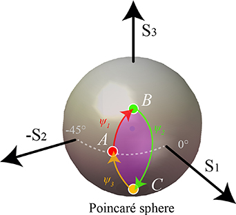
Figure 2. Action of the three SLMs represented on the Poincaré sphere for a linear retardance eigenmode.  ,
,  , and
, and  represent respectively the phase settings of the three SLMs. Point A represents the polarisation eigenmode of the system.
Download figure:
Standard image High-resolution image
Figure 3. Geometrical derivation for calculation of the phase setting  of SLM2.
Download figure:
Standard image High-resolution imageWhere we have set  .
.
The choice of closed path is not unique, as the point B can be chosen to lie on any point on the circle that passes through A and is in a plane perpendicular to the axis  . This degree of freedom permits control of the equivalent retardance of the system. As the retardance is the difference in phase between the two eigenvalues, the position of B can be chosen to ensure that the system retardance is equivalent to that of the desired waveplate.
3.2. Linear retarders—retardance
We show in this section how one can obtain the value of  necessary to implement a chosen retardance. Using the condition
  , from equation (12), we can obtain the following relationship between the retardance
  of the three-SLM system and other parameters:
From equation (13) we have

Through a sequence of trigonometric manipulations (see appendix  to obtain the relationship:
We hence find that
We can also find an explicit expression relating  directly to the retardance and waveplate angle as (see appendix
So that
We therefore have explicit expressions for the SLM settings in terms of the desired retarder's properties.
Aside from the special cases where  , which are explained below, there is a one-to-one mapping between
  and
and  , in the range
  . Hence, it is clear that any retardance in the range
  can be achieved with an appropriate choice of
  . Furthermore, retardances in the range
  are possible when one considers the full range of parameter values that are accessible.
Figure 4 (along with supplementary video 1 (available online at stacks.iop.org/JOPT/23/065602/mmedia)) shows how the retardance  varies with the choice of the system parameters
  and
and  , as plotted on the surface of the PS. The explicit expression for the retardance in terms of
 and
and  is, from equation (16),

Figure 4. The colour at a point B on the Poincaré sphere represents the retardance in radians of the system for that choice of B. The position of the point is parameterised by the variables  and
and  . The thick grey circle shows the 'equator' where
  , which is also the locus for
  . The dotted line shows the locus of
  . See also supplementary video 1.
Download figure:
Standard image High-resolution imageThe relationship between the retardance  and the settings of the three SLMs
  ,
,  and
and  can also be expressed geometrically by calculating the total area of spherical triangles formed by points A, B, C and the optical axes of the three SLMs on a PS (see appendix
3.3. Linear retarders—dynamic phase
The derivation above shows that the three SLM system can mimic the retardance of an arbitrary linear waveplate. However, the dynamic phase introduced by the system—given by  —cannot be independently chosen. For single retarders that modulate the whole beam uniformly, this phase offset is not important. However, for an adaptive system that modulates the beam differently across its profile, phase offsets that differ between pixels correspond to wavefront aberration. Consequently, for full vectorial control we require an additional adaptive element to adjust the overall phase. The DM is included in the system for this purpose.
As the determinant of a matrix is given by the product of its eigenvalues, the dynamic phase can be calculated from the Jones matrix  based upon the SLM retardances using
  and
and ![${\psi _2} = 2{\text{atan}}\left[ {\tan \left( {2\theta } \right)\sin \left( \beta \right)} \right]$](https://content.cld.iop.org/journals/2040-8986/23/6/065602/revision3/joptabed33ieqn69.gif) to give the expression
to give the expression

This phase would need to be compensated by the DM in order that the combined system behave as the modelled retarder. Figure 5 (along with supplementary video 2) shows how  varies with the choice of the system parameters
  and
and  , as plotted on the surface of the PS.
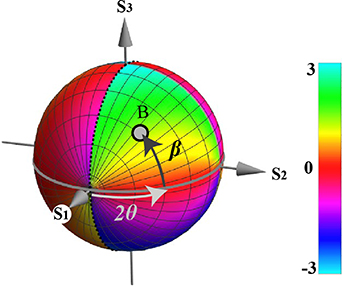
Figure 5. The colour at a point B on the Poincaré sphere represents the dynamic phase of the system for that choice of B. The position of the point is parameterised by the variables  and
and  . The thick grey circle shows the 'equator' where
  , which is also the locus for
  . The dotted line shows the locus of
  . See also supplementary video 2.
Download figure:
Standard image High-resolution image3.4. Linear retarders—special cases
There are two special cases of linear retarders that need to be addressed: one with an x-oriented axis, which would be co-aligned with the primary axis of SLM1 (and SLM3); another where the axis is at 45° and hence aligned with the axis of SLM2. For the x-oriented retarder, we can set  and the retardance would be
  . In this case, no path is traced out on the PS, but the settings of SLM1 (and/or SLM3) can be used to access all retardances.
For the 45° retarder, we set  and have freedom to control the retardance purely using
  . Other SLM settings are possible for
  , but in this case the retardance is always limited to
  radians.
4. Elliptical retarders implemented through the multiple SLM system
4.1. Elliptical retarders—eigenvectors
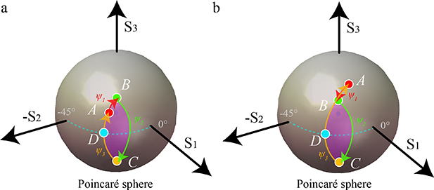
For a general elliptical retarder, we have to consider eigenvectors corresponding to any arbitrary point A on the PS. We can use a geometric construction for the path ABCA that is similar that introduced above for the linear retarders. In this case though, the point A does not lie on the equator. There are two possibilities for the path shape, dependent upon whether the action of SLM1 is to move the state towards or away from the equator. These two cases are illustrated in figure 6. In case 1, the path shape is the same as for the linear retarder in the previous section, but with point A not lying on the equator. In case 2, the path AB due to SLM1 is retraced as part of the path CA due to SLM3.
Figure 6. Action of the three SLMs represented on the Poincaré sphere for elliptical retardance eigenmodes. Parts (a) and (b) represent two possible configurations of the points A and B.  ,
,  , and
, and  represent respectively the phase settings of the three SLMs. Point A in each case represents the polarisation eigenmode of the system.
Download figure:
Standard image High-resolution image
In this configuration  . We define D to be the point at which the arc AC crosses the equator, then the angle
  subtended by DB at the
  axis is given by
where  and
and  are the elements of the Stokes vector at B. We also define
  to be the angle subtended by DA at the
  axis, such that
The arc ADC lies in a plane perpendicular to the  axis, so the point D would represent a linear polarisation at orientation
  , where
  is the first element of the normalised Stokes vector at A. Note that
  . We can therefore determine that the retardance of SLM2 should again be given by

As for the linear retarder above, we have one degree of freedom—equivalent to the choice of the position of point B—that enables us to control the retardance of the equivalent waveplate.
4.2. Elliptical retarders—retardance
When using the three-SLM system to simulate a single elliptical retarder, the same relationships between the desired retardance and  and
and  as derived in section 3 are again valid:
We can therefore use this to derive the settings for the three SLMs. Using  we obtain the SLM settings as

and
As the retardance is dependent only on the choice of point B and hence on  and
and  , the plot of figure 4 is also valid for elliptical retarders.
4.3. Elliptical retarders—dynamic phase
Following the derivation in section 3, we calculate the dynamic phase from the Jones matrices based upon the SLM retardances using  ,
, ![${\psi _2} = 2{\text{atan}}\left[ {\tan \left( {2\theta } \right)\sin \left( \beta \right)} \right]$](https://content.cld.iop.org/journals/2040-8986/23/6/065602/revision3/joptabed33ieqn104.gif) , and
, and  to give the equivalent expression

As the expression for dynamic phase is identical to that obtained for linear retarders, the plot of figure 5 is also valid for elliptical retarders.
4.4. Elliptical retarders—special cases
For circular polarisation eigenmodes, where the point A lies on the  axis, we can set
  and
and  . The action of SLM1 would be to transform an eigenmode input to a state on the
  axis. SLM2 would then apply the arbitrarily chosen phase shift
  . SLM3 would transform this state back to the original state at point A. The retardance of the overall system would be equal to
  .
.
5. Discussion
Many optical systems can suffer from errors introduced into the polarisation state of the light through, for example, stressed optical elements, dielectric coatings, Fresnel transmission and reflection effects at surfaces, in addition to bulk birefringence of optical materials. These effects would generally be variant across the beam profile, as modelled by the state of the Jones pupil that represents a spatially variant retarder. In applications where these effects are variable over time, their correction would require adaptive adjustment and hence an arrangement of polarisation and phase state modulators, such as the multiple SLM systems described in this paper. Note that compensation of vectorial aberrations in this way would be independent of the polarisation state of the input light, as the compensator would induce the conjugate retardance effect to the disturbance. The systems described in this paper could therefore form the corrector device for polarisation and phase aberrations in future vectorial adaptive optics systems.
In order to derive control schemes for vectorial AO, it is necessary to employ a suitable mathematical framework for description of vectorial aberrations and their correction. For non-diattentuating and non-depolarising systems, the vectorial aberrations can be described by spatially variant retarders in the form of Jones matrices. If the desired retardance is specified in terms of orientation and retardance, then the results in this paper can be used to obtain the SLM settings required to reproduce the complex retarder via the SLM system.
As we have also derived the expressions for the dynamic phase introduced by the multiple SLM system for any retardation, we can use this to determine the phase setting for the DM that would compensate any addition phase shifts. Of course, this same DM could also be used to compensate for phase aberrations that are introduced into the system.
In practice, the performance of SLM based compensation systems would be affected by limitations of practical liquid crystal devices, such as pixellation, fill-factor and reflection efficiency of the SLMs. However, within these limitations, the configuration modelled here has the potential to operate with high throughput efficiency. The practicality of this is backed up by demonstrations in the existing literature that have used multiple SLMs for beam modulation [12–14, 20–22]. Implementation of such a system with reflective SLMs is feasible, but cumbersome. Future implementations might use a stack of simpler transmission mode modulators tailored, for example, to low-order vectorial aberrations encountered in the system. The models derived in this paper could also be applied to these systems.
6. Conclusion
In this paper, we have presented a method using a sequence of SLMs that can compensate the vectorial aberrations introduced by an arbitrary retarder, regardless of the input polarisation states of the beam. By considering the geometry of transformations on the PS induced by a sequence of three SLMs, we have created a method for determining the SLM settings that reproduce the effects of an arbitrary spatially variant retarder. Including a further adaptive element, in the form of a DM, permits compensation of the dynamic phase introduced by the multiple SLM system. This combination of adaptive elements could form the basis of an optically efficient correction device for vectorial aberrations in an adaptive optics scheme.
This is an advance on our previous work [23], which addressed the ability to use a multiple SLM system to convert between two specified vectorial states. The solution to this state conversion problem is not unique, as multiple SLM arrangements can perform the same conversion. Furthermore, the methods presented here will perform compensation for all possible PS states simultaneously, by effectively creating a retarder conjugate to that causing the vectorial aberration. For this reason, the method presented here will be applicable even to vectorial aberrations of complex vector beams that contain multiple polarisation states, such as full Poincaré beams.
Acknowledgments
This work was supported by funding from the European Research Council (ERC) under the European Union's Horizon 2020 research and innovation programme (AdOMiS, Grant Agreement No. 695140).
Appendix A.: Derivation of expression for β
We derive here the equations for obtaining  from the retardance
  and orientation
  of the desired retarder. From equation (14), we have
From equation (15) we have
which can be recast using trigonometric manipulations as
Through squaring both sides of equation (31) and substitution for  , we obtain the two equivalent expressions
Using the identity  we obtain:
which leads to the result
If  is restricted to the range
  then there are two solutions for the retardance and angle corresponding to 90° rotations of the retarder.
Appendix B.: Derivation of expression for Ψ 2
From appendix A we have the two expressions:
Combining these by dividing the second equation by the first we obtain

We can remove the dependence on  using
using
which leads to the expression
which can be simplified to

thus providing an expression for the retardance required for the second SLM in terms of the retardance and angle of the desired retarder.
Appendix C.: Pancharatnam models for retardance and dynamic phase
Appendix. Linear retarders
The total phase introduced by the three-SLM system can be calculated using following expressions [24]

where  ,
,  and
and  are the phases introduced by each SLM and
  is a Pancharatnam phase term. These can be calculated using the areas of spherical triangles as
where  represents the area of the spherical triangle formed between the points X, Y and Z;
  ,
,  and
and  are the normalised Stokes vectors representing points A, B and C;
  is the vector representing the non-modulating eigenmode of SLM1 (or equivalently of SLM3), which points along the
  axis in the negative direction;
  is the vector representing the non-modulating eigenmode of SLM2, which points along the
  axis in the negative direction.
Using the shorthand notation  and
and  , we can define the normalised Stokes vectors as
Then we find that
Where we have used symmetry to find that the phases from SLM1 and SLM3 must be identical. We find further that
As  was chosen to be an eigenvector of the system, then the phase
  must be the phase of the corresponding eigenvalue
  .
.
To obtain the equivalent phases for the opposite eigenvector passing through the same three-SLM system, we replace  ,
,  , and
, and  by the diametrically opposed vectors. The resulting phases are
The eigenvalue corresponding to this eigenvector is therefore  , where

The retardance of the three-SLM system is thus given by

where the asterisk represents the complex conjugate.
As the determinant of a matrix is given by the product of its eigenvalues, we can use the geometrical model to calculate the dynamic phase as

Appendix. Elliptical retarders
Here, the normalised Stokes vectors are given by

where only the definition of  has changed
Using these definitions for the individual phase terms, we can obtain the retardance of the three-SLM system as

Following the derivation in the section for linear retarders, we calculate the dynamic phase introduced by the three-SLM system as