the Creative Commons Attribution 4.0 License.
the Creative Commons Attribution 4.0 License.
 | 04 Jun 2021
Efficient multi-angle polarimetric inversion of aerosols and ocean color powered by a deep neural network forward model
Bryan A. Franz
Kirk Knobelspiesse
Peng-Wang Zhai
Vanderlei Martins
Sharon Burton
Brian Cairns
Richard Ferrare
Joel Gales
Otto Hasekamp
Yongxiang Hu
Amir Ibrahim
Brent McBride
Anin Puthukkudy
P. Jeremy Werdell
Xiaoguang Xu
NASA's Plankton, Aerosol, Cloud, ocean Ecosystem (PACE) mission, scheduled for launch in the timeframe of 2023, will carry a hyperspectral scanning radiometer named the Ocean Color Instrument (OCI) and two multi-angle polarimeters (MAPs): the UMBC Hyper-Angular Rainbow Polarimeter (HARP2) and the SRON Spectro-Polarimeter for Planetary EXploration one (SPEXone). The MAP measurements contain rich information on the microphysical properties of aerosols and hydrosols and therefore can be used to retrieve accurate aerosol properties for complex atmosphere and ocean systems. Most polarimetric aerosol retrieval algorithms utilize vector radiative transfer models iteratively in an optimization approach, which leads to high computational costs that limit their usage in the operational processing of large data volumes acquired by the MAP imagers. In this work, we propose a deep neural network (NN) forward model to represent the radiative transfer simulation of coupled atmosphere and ocean systems for applications to the HARP2 instrument and its predecessors. Through the evaluation of synthetic datasets for AirHARP (airborne version of HARP2), the NN model achieves a numerical accuracy smaller than the instrument uncertainties, with a running time of 0.01 s in a single CPU core or 1 ms in a GPU. Using the NN as a forward model, we built an efficient joint aerosol and ocean color retrieval algorithm called FastMAPOL, evolved from the well-validated Multi-Angular Polarimetric Ocean coLor (MAPOL) algorithm. Retrievals of aerosol properties and water-leaving signals were conducted on both the synthetic data and the AirHARP field measurements from the Aerosol Characterization from Polarimeter and Lidar (ACEPOL) campaign in 2017. From the validation with the synthetic data and the collocated High Spectral Resolution Lidar (HSRL) aerosol products, we demonstrated that the aerosol microphysical properties and water-leaving signals can be retrieved efficiently and within acceptable error. Comparing to the retrieval speed using a conventional radiative transfer forward model, the computational acceleration is 103 times faster with CPU or 104 times with GPU processors. The FastMAPOL algorithm can be used to operationally process the large volume of polarimetric data acquired by PACE and other future Earth-observing satellite missions with similar capabilities.


Atmospheric aerosols are tiny particles suspended in the atmosphere, such as dust, sea salt, and volcanic ash, that play important roles in air quality (Shiraiwa et al., 2017; Li et al., 2017) and Earth's climate (Boucher et al., 2013). Aerosols influence the Earth's reflectivity directly through scattering and absorption of solar light and indirectly through interactions with clouds. The radiative forcing from aerosols is one of the main uncertainties in studies of global climate change (Boucher et al., 2013). When deposited into ocean waters, aerosols also contribute to the availability of nutrients needed for phytoplankton growth and thereby influence ocean ecosystems (Westberry et al., 2019). Accurate knowledge of aerosol optical properties is also important for atmospheric correction in ocean color remote sensing, wherein the spectral water-leaving radiances are retrieved by subtracting the contributions of the atmosphere and ocean surface from the spaceborne or airborne measurements made at the top of atmosphere (TOA; Mobley et al., 2016). The resulting water-leaving signals provide valuable information to derive biogeochemical quantities for monitoring the global ocean ecosystem (Dierssen and Randolph, 2013) and for quantifying ocean biochemical processes (Platt et al., 2008). Accurate assessments of aerosol optical and microphysical properties are thus important for both atmospheric and oceanic studies.
Multi-angle polarimeters (MAPs) measure polarized light at continuous or discrete spectral bands and at multiple viewing angles, providing rich information on aerosol optical and microphysical properties (Mishchenko and Travis, 1997; Chowdhary et al., 2001; Hasekamp and Landgraf, 2007; Knobelspiesse et al., 2012). The Polarization and Directionality of the Earth's Reflectances (POLDER) instrument pioneered the spaceborne MAP, which was hosted on Advanced Earth Observing Satellite missions (ADEOS-I; 1996–1997 and ADEOS-II; 2002–2003) and the Polarization and Anisotropy of Reflectances for Atmospheric Sciences coupled with Observations from a Lidar (PARASOL; 2004–2013) mission (Tanré et al., 2011). The Hyper-Angular Rainbow Polarimeter (HARP) CubeSat, a small satellite with 3U (10 cm × 10 cm × 30 cm) volume, was launched from the International Space Station on February of 2020 and has captured scientific images (UMBC Earth and Space Institute, 2021). Several satellite missions plan to carry MAP instruments, which are scheduled to be launched in the timeframe of 2023–2024, including the European Space Agency's (ESA) Multi-viewing Multi-channel Multi-polarisation Imager (3MI) on board the MetOp-SG satellites (Fougnie et al., 2018), the National Aeronautics and Space Administration's (NASA) Multi-Angle Imager for Aerosols (MAIA) (Diner et al., 2018), and Plankton, Aerosol, Cloud, ocean Ecosystem (PACE) (Werdell et al., 2019) missions. A thorough review of the MAP instruments and algorithms can be found in Dubovik et al. (2019).
The PACE mission will carry a hyperspectral scanning radiometer named the Ocean Color Instrument (OCI) and two MAPs: a next-generation UMBC (University of Maryland, Baltimore County) Hyper-Angular Rainbow Polarimeter (HARP2) (Martins et al., 2018) and the SRON (Netherlands Institute for Space Research) Spectro-Polarimeter for Planetary EXploration one (SPEXone) (Hasekamp et al., 2019a). OCI will provide continuous spectral measurements from the ultraviolet (340 nm) to near-infrared (890 nm) with full width at half maximum of 5 nm resolution and sampling every 2.5 nm, plus a set of seven discrete shortwave infrared (SWIR) bands centered at 940, 1038, 1250, 1378, 1615, 2130, and 2260 nm. SPEXone performs multi-angle measurements at five along-track viewing angles of 0∘, , and , with a surface swath of 100 km and a continuous spectral range spanning 385–770 nm at resolutions of 2–3 nm for intensity and 10–40 nm for polarization (Rietjens et al., 2019). HARP2 is a wide field-of-view imager that measures the polarized radiances at 440, 550, 670, and 870 nm, where the 670 nm band will measure 60 viewing angles and the other bands 10 viewing angles, with a swath of 1556 km at nadir on the Earth's surface. To facilitate cross calibrations and validations, a PACE Level-1C common data format has been developed, with the purpose of projecting all three PACE instruments onto an uniform spatial grid (Plankton, Aerosol, Cloud, ocean Ecosystem – PACE, 2020). The PACE instruments will provide an unprecedented opportunity to improve the characterization of the atmosphere and ocean states (Remer et al., 2019a, b; Frouin et al., 2019).
To retrieve the aerosol information from polarimetric measurements over oceans, several advanced aerosol retrieval algorithms have been developed for both airborne and spaceborne MAPs, such as POLDER/PARASOL(Hasekamp et al., 2011; Dubovik et al., 2011, 2014; Li et al., 2019; Hasekamp et al., 2019b; Chen et al., 2020), the Airborne Multiangle SpectroPolarimetric Imager (AirMSPI) (Xu et al., 2016, 2019), SPEX airborne (the airborne version of SPEXone) (Fu and Hasekamp, 2018; Fu et al., 2020; Fan et al., 2019), the Research Scanning Polarimeter (RSP) (Chowdhary et al., 2005; Wu et al., 2015; Stamnes et al., 2018; Gao et al., 2018, 2019, 2020), and the Directional Polarimetric Camera (DPC) on board Gaofen-5 (Wang et al., 2014; Li et al., 2018). The retrieval algorithms are mostly based on iterative optimization approaches that utilize vector radiative transfer (RT) models as the forward model. The high computational costs of the RT simulations pose great challenges in the operational processing of the large data volumes acquired by the MAP imagers. To alleviate this issue, the SPEX team represented the polarimetric reflectance for an open-ocean system using a deep neural network (NN) and coupled it with a radiative transfer model for the atmosphere (Fan et al., 2019). This hybrid forward model avoids the direct calculation of the scattering and absorption properties inside the ocean and still maintains high accuracy, therefore enabling sufficient efficiency for SPEXone data retrieval. For coastal waters, Mukherjee et al. (2020) developed a NN model to predict the polarimetric reflectance associated with complex water optical properties. This NN model can be combined with a flexible atmosphere model for MAP aerosol retrievals over complex waters.
For non-polarimetric remote sensing studies, several NN approaches have been developed to derive aerosol and ocean properties simultaneously (Fan et al., 2017; Shi et al., 2020, and references therein). Fan et al. (2017) developed NN models to directly invert the aerosol optical depth (AOD) and remote sensing reflectance Rrs(λ) (sr−1) from the NASA Moderate Resolution Imaging Spectroradiometer (MODIS) measurements. Shi et al. (2020) developed a NN radiative transfer scheme for coupled atmosphere and ocean systems including both open and coastal waters, which is then applied in an optimal estimation algorithm for the Cloud and Aerosol Imager-2 (CAI-2) hosted on the Greenhouse gases Observing Satellite-2 (GOSAT-2).
A number of NN models have been developed to directly invert the aerosol microphysical properties from MAP measurements. Di Noia et al. (2015) discusses the NN employed to retrieve aerosol refractive index, size, and optical depth (AOD) from groundSPEX (a ground version of SPEX instrument) measurements. Di Noia et al. (2017) developed a NN inversion method for airborne MAP measurement over land from RSP. In both works, the results from the NN inversion are further used as initial values for iterative optimization, and both efficiency and the retrieval accuracy are shown to be improved. Using NN to conduct direct inversion is efficient, but it is often viewed as a black box, and it is difficult to account for measurement uncertainties. The combination of a NN inversion with an iterative optimization method shows promise for MAP retrievals.
Even with such ample progress, it is still challenging for current state-of-the-art algorithms to process MAP data operationally through iterative optimization. In this work, we present a joint retrieval algorithm for aerosol properties and water-leaving signals that uses a deep NN model to replace the radiative transfer forward model for simulation of the polarimetric reflectances. This approach is one step further than Fan et al. (2019), as both the atmospheric and oceanic radiative transfer processes are represented by the NN. The NN forward model is then used in an iterative retrieval algorithm that is significantly more computationally efficient than approaches that use traditional radiative transfer. The benefits of using a NN model as the forward model in retrieval algorithms can be summarized as follows with details provided in later sections.
-
Fast. NN models involve matrix operations that can be evaluated efficiently.
-
Accurate. Given sufficient training data volumes and accuracies, NN models can be trained with high precision.
-
Differentiable. The Jacobian matrix of NN models can be represented analytically and therefore further improves efficiency and accuracy in retrievals.
-
Transferable. The parameters of a NN can be exported and implemented into existing retrieval algorithms.
The retrieval algorithm we developed is called FastMAPOL, which is evolved from the well-validated Multi-Angular Polarimetric Ocean coLor (MAPOL) algorithm (Gao et al., 2018, 2019, 2020) by replacing its forward model with NN models. To validate the retrieval algorithm, we applied FastMAPOL to both synthetic and field measurements from AirHARP (the airborne version of HARP2 and HARP CubeSat) for the Aerosol Characterization from Polarimeter and Lidar (ACEPOL) campaign in 2017 (Knobelspiesse et al., 2020). The synthetic AirHARP data are a supplement of the field measurements with a wider range of aerosol and ocean optical properties, as well as solar and viewing geometries. The AODs derived from coincident High Spectral Resolution Lidar (HSRL, Hair et al., 2008) and Aerosol Robotic Network (AERONET, Holben et al., 1998) measurements are used to evaluate the performance of the AOD retrieval from the AirHARP field measurements. Using the retrieved aerosol properties, atmospheric correction is applied to the AirHARP measurements to derive the water-leaving signal at four AirHARP bands. The retrieved aerosol products from MAP can also assist hyperspectral atmospheric correction on instruments such as PACE OCI as previously demonstrated using the aerosol properties retrieved from RSP and hyperspectral measurements from SPEX airborne (Gao et al., 2020; Hannadige et al., 2021). Retrieval uncertainties of both aerosol and water-leaving signals under various aerosol loadings are also discussed in this study. The retrieval algorithm powered by the NN forward model provides a practical approach for operational applications of polarimetric aerosol and ocean color retrieval for PACE, as well as other satellite missions that utilize polarimeters in the retrieval of geophysical properties from Earth observations.
The paper is organized into seven sections: Sect. 2 reviews the retrieval algorithm and its radiative transfer forward model, Sect. 3 discusses the training and accuracy of the NN forward model, Sect. 4. applies the NN forward model to aerosol and water-leaving signal retrievals from the synthetic AirHARP data, Sect. 5. discusses the retrievals on AirHARP field measurements from the ACEPOL campaign, and Sects. 6 and 7 provide discussions and conclusions.
In this section, we will discuss the MAPOL retrieval algorithm based on multi-angle polarimetric measurements and the associated radiative transfer forward model. The retrieval algorithm has been validated using both synthetic data (Gao et al., 2018) and RSP field measurements (Gao et al., 2019, 2020). To apply the retrieval algorithm to AirHARP measurements, we will first discuss the AirHARP instrument characteristics.
AirHARP measures the total and linearly polarized radiance at 60 viewing angles at the 660 nm band and at 20 viewing angles at the 440, 550, and 870 nm bands. Different from AirHARP, HARP2 reduces the number of viewing angles to 10 at 440, 550, and 870 nm and maintains 20 viewing angles at 660 nm in order to fulfill the bandwidth requirement and preserve information content as much as possible. HARP instruments (AirHARP, HARP CubeSat, and HARP2) use a modified three-way Phillips prism located after the front lens to split the incident light into the three orthogonal linear polarization states (0∘, 45∘, and 90∘), which can be recombined to obtain the Stokes parameters Lt, Qt, and Ut at the observational altitude (Puthukkudy et al., 2020). Circular polarization (Stokes parameter V) is not measured by any of the polarimeters in ACEPOL as it is negligible for atmospheric studies (Kawata, 1978). We use the total measured reflectance (ρt(λ)) and degree of linear polarization (DoLP, Pt(λ)) at the height of the aircraft with spectral dependencies hereafter implied, which are defined as
where F0 is the extraterrestrial solar irradiance, μ0 is the cosine of the solar zenith angle, and r is the Sun–Earth distance correction factor in astronomical units.
Based on the MAP measurements, the MAPOL retrieval algorithm is developed to derive both the aerosol properties and the water-leaving signal simultaneously. The retrieval algorithm minimizes the difference between the MAP measurements and the forward model simulations computed from vector radiative transfer simulations (Zhai et al., 2009, 2010). By assuming the measurement and modeling uncertainties follow Gaussian statistical distributions, the retrieval parameters can be estimated through Bayesian theory using the cost function χ2 to quantify the difference between the measurement and the forward model simulation (Rogers, 2000):
where ρt and Pt are the measured reflectance and DoLP as defined in Eqs. (1) and (2), and and are the corresponding quantities computed from the forward model. The state vector x contains all retrieval parameters, such as the aerosol size and refractive indices; the subscript i stands for the index of the measurements at different viewing angles and wavelengths; and N is the total number of the measurements used in the retrieval. For AirHARP measurements, the maximum value of N is 240, twice of the total number of viewing angles. The total uncertainties of the reflectance and DoLP used in the algorithm are denoted as σρ and σP, which are contributed by both the measurement uncertainties σm and the forward model uncertainties σf (more details in Sect. 3.3):
One important component of σm is the calibration uncertainty. AirHARP was calibrated in the lab with an accuracy of 3 %–5 % for reflectance and 0.005 for DoLP (McBride et al., 2019). In-flight uncertainty for the AirHARP DoLP is conservatively estimated to be at most 0.01 without an onboard calibrator. In this study, we adopted the calibration uncertainty for reflectance as and for DoLP as for all four bands. The accuracy of the HARP2 measurements can be further improved through onboard calibration (McBride et al., 2020; Puthukkudy et al., 2020). In this study, we considered the total measurement uncertainties as the contributions only from the calibration (σcal):
However, other contributions such as spatial variability of the geophysical properties may also contribute to the measurement uncertainties, which will be discussed in Sect. 5. Furthermore, noise correlation is an import influence on the retrieval accuracy (Knobelspiesse et al., 2012) that is ignored in this study due to the lack of knowledge on this characteristic for AirHARP.
As observed by AirHARP (Puthukkudy et al., 2020) and RSP measurements (Gao et al., 2020), the sunglint angular pattern cannot be well modeled by an isotropic Cox–Munk model. Using these data will require characterization of the corresponding measurement and model uncertainties. To minimize the impact of sunglint in our discussions, we removed the signals within an angle range of 0∘ to 40∘ relative to the solar specular reflection direction.
The forward model uncertainties σf include the uncertainties of the radiative transfer calculation and uncertainties due to the incompleteness of the model to describe the system. However, the latter are difficult to quantify; we will discuss the possible sources for them in the next section. For convenience, we will only consider the uncertainties of the NN forward model (σNN) and the radiative transfer simulation used for generating the NN training data (σRT) as
σNN is evaluated by comparing with synthetic multi-angle AirHARP measurements discussed in Sect. 3.3.
To fully utilize the information contained in the AirHARP measurements, the forward model needs to achieve an accuracy level much better than the measurement uncertainties. This becomes the goal of the NN training in the next section. Detailed comparisons of the forward model uncertainties and the measurement uncertainties will be provided in the next section. To minimize the cost function defined in Eq. (3), we use an optimization method, called the subspace trust-region interior reflective (STIR) approach (Branch et al., 1999) as implemented in the Python SciPy package (Virtanen et al., 2020), to solve the state parameters x iteratively. The method is based upon the Levenberg–Marquardt method (Moré, 1978) and shows good stability for the boundary constraints.
2.1 Forward model
We used a vector radiative transfer model based on the successive order of scattering method for coupled atmosphere and ocean systems (Zhai et al., 2009, 2010) to model the measured reflectance and DoLP. The atmosphere is configured as three layers: a top molecular layer above the aircraft, a molecular layer below the aircraft in the middle, and an aerosol and molecular mixing layer on the bottom with a height of 2 km. Aerosols are assumed to be uniformly distributed in the mixing layer as shown in the left panel of Fig. 1. The same vertical structure of the atmosphere was successfully used in the inversion of RSP data (Gao et al., 2019, 2020).

Figure 1Panel (a) shows the coupled atmosphere and ocean system used in FastMAPOL including the atmosphere, ocean surface, and ocean body. Panel (b) represents a system used for atmospheric correction which only has atmosphere and ocean surface without scattering in the ocean body. The atmospheres in both systems are modeled as the same three layers. TOA indicates the top of the atmosphere. The bottom of the atmosphere (BOA) and the top of the ocean (TOO) indicate the locations just above and below the ocean surface, respectively. All quantities shown in the figures need to be computed from the forward model and represented by the NN for efficient calculations. Symbols are defined in Table 1.
The atmospheric surface pressure is assumed to be 1 atm (standard atmosphere pressure), which is consistent with the value discussed in Sect. 5. Anisotropic molecular Rayleigh scatterings are accounted for in Hansen and Travis (1974). The molecular absorption properties are computed by the hyperspectral line-by-line atmospheric radiative transfer simulator (ARTS) (Buehler et al., 2005) with the molecular absorption parameters of oxygen, water vapor, methane, and carbon dioxide from the HITRAN database (Gordon et al., 2017). The gas absorption of ozone and nitrogen dioxide are from Gorshelev et al. (2014), Serdyuchenko et al. (2014), and Bogumil et al. (2003), respectively. The hyperspectral absorption coefficients are then averaged within the instrument spectral response function and used in the multiple scattering radiative transfer simulation (Zhai et al., 2009, 2010, 2018). The molecular profile used is the US standard atmospheric constituent profiles (Anderson et al., 1986). Ozone is the most important gas that influences the absorption transmittance at the AirHARP bands of 550 and 660 nm. For the application to AirHARP measurements in ACEPOL, we use the ozone column density as a free parameter with values from the Modern-Era Retrospective analysis for Research and Applications, Version 2 (MERRA-2) developed by NASA's Global Modeling and Assimilation Office (Gelaro et al., 2017) to rescale the molecular absorption optical depth calculated under the abovementioned standard atmospheric profile.
Aerosols are diverse in size, composition, and morphology. To capture their variation in the atmosphere, we modeled the size and refractive index for both fine and coarse modes. The aerosol size is represented by the volume density distribution as a combination of five lognormal distributions:
where Vi is the column volume density for each submode; the mean radius ri is fixed with values of 0.1, 0.1732, 0.3, 1.0, and 2.9 µm; and the standard deviation σi is fixed with values of 0.35, 0.35, 0.35, 0.5, and 0.5 (Dubovik et al., 2006; Xu et al., 2016). The first three submodes are categorized as the fine-mode aerosol, while the last two submodes are the coarse mode. All aerosols are assumed to be spherical in the current forward model. The nonspherical particle shape is important in the aerosol model (Dubovik et al., 2006) and will be considered in future studies. The aerosol refractive index spectra for the fine and coarse modes are represented by the principal component analysis in MAPOL (Wu et al., 2015; Gao et al., 2018) as
where p1(λ) is the first-order principal component computed from the aerosol refractive index dataset including water, sea salt, dust-like particles, biomass burning, soot, sulfate, water-soluble aerosols, and industrial aerosols (Shettle and Fenn, 1979; d'Almeida et al., 1991). m0 and α1 are two coefficients to determine the spectrum. For the application to AirHARP bands, p1(λ) for the real part of the refractive index is approximately spectrally flat for both the fine- and coarse-mode aerosols within the AirHARP spectral range. We further assume the spectral shape for the imaginary refractive spectra is also flat. Two parameters can be combined into one to represent the refractive index. Hereafter, we only refer one independent parameter for each refractive index spectrum. Therefore, only four independent parameters are required to determine the real and imaginary refractive index spectra for the fine and coarse modes. With the aerosol size and refractive index, the polarimetric single scattering properties are modeled by the Lorenz–Mie theory and computed by the code developed by Mishchenko et al. (2002).
For the ocean layer shown in Fig. 1, two ocean bio-optical models are implemented in the forward model of MAPOL: one with chlorophyll a concentration (Chl a; mg m−3) as the single parameter applicable to open-ocean optical properties and the other with seven parameters more suitable to fully describe complex coastal waters (Gao et al., 2019). Since the waters are generally clear within the ocean scenes in this study (Gao et al., 2020), an open-ocean model is used for both NN training and retrievals. The optical properties of open-ocean waters include contributions from pure seawater, colored dissolved organic matter (CDOM), and phytoplankton, where the CDOM and phytoplankton absorption coefficients as well as the phytoplankton scattering coefficient and phase function are parameterized by Chl a (Gao et al., 2019). A complex costal water model for NN trainings will be investigated in separate studies. The ocean surface roughness is modeled by the isotropic Cox–Munk model with a scalar wind speed. Whitecap is not considered in the current study.
In summary, the parameters used to represent the forward model include five volume densities (one for each submode); four independent parameters for the refractive indices of fine and coarse modes; and one parameter for wind speed, ozone column density, and Chl a, respectively. Three additional geometric parameters are used to set up the system, including the solar zenith angle, viewing zenith angle, and relative viewing azimuth angle. Therefore, it requires a total of 15 parameters to conduct the radiative transfer calculation, with a total of 11 independent state parameters that can be retrieved from optimizing the cost function as defined in Eq. (3).
2.2 Remote sensing reflectance
An important task for the joint retrievals is to obtain the water-leaving signal, which is often represented in ocean color studies by the spectral remote sensing reflectance defined as , where is the downwelling irradiance and is the water-leaving radiance just above the ocean surface (Mobley et al., 2016). The remote sensing reflectance can be derived from the water-leaving reflectance reaching the sensor (ρw) via
where θ0 and θv are the solar and viewing zenith angles, and ϕv is the relative viewing azimuth angle. ρw represents the signals originating from scattering in the ocean that reached the sensor, which can be derived from the atmospheric correction process as
where ρt is the measured total reflectance as defined in Eq. (1), and is the reflectance from a system with only atmosphere and ocean surface (Mobley et al., 2016) as represented in the right panel of Fig. 1. The same formalism has been used to derive Rrs from RSP measurements Gao et al. (2019, 2020).
Table 1Definition of the symbols for the quantities computed from the forward model (indicated by the superscript f) as shown in Fig. 1.
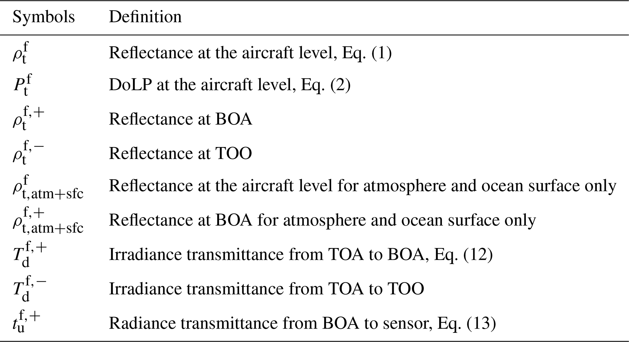
The downwelling irradiance transmittance is for the solar irradiance from TOA to the surface, and the upwelling radiance transmittance is for the water-leaving radiance from BOA to the sensor (Gao et al., 2019). Both and are denoted in Fig. 1 and represented as follows:
where and are reflectance just above ocean surface also denoted in Fig. 1 and Table 1.
To remove the dependency of Rrs on the solar and viewing geometries, a bidirectional reflectance distribution function (BRDF) correction CBRDF is applied to adjust Rrs to the observation with a zenith sun and a nadir viewing direction as defined by Morel et al. (2002):
accounts for reflection and refraction effects when light propagates through the ocean interface. () is the direction of the upwelling radiance beneath the sea surface, where is defined through Snell's law:
with water refractive index nw. CBRDF in its original form is defined using the radiance and irradiance just below the ocean surface (Morel et al., 2002); here we have converted all quantities into the radiance reflectance and the irradiance transmittance similar to Eqs. (1) and (12).
To compute the remote sensing reflectance from the multi-angle AirHARP measurement, we only consider the reflectance at the minimum viewing zenith angle for each wavelength and apply the atmospheric correction and BRDF correction as discussed above. For (), the factor is approximately a constant value of 1, but for larger θv angles, the ratio increases with both wind speed and θv (Morel and Gentili, 1996; Morel et al., 2002). In this study we ignored the factor in Eq. (14), which will not impact Rrs calculation from synthetic data due to the small viewing zenith angle used but may cause underestimation of Rrs at the edge of the image, as will be discussed in Sects. 4 and 5. All quantities denoted in Fig. 1 and Table 1 need to be determined for the forward model and the calculation of remote sensing reflectance and will be represented by NN models.
Deep NN models are developing rapidly due to the advancement in machine-learning infrastructure and demands in broad applications (Goodfellow et al., 2016) and are demonstrated to be efficient in approximating physical functions (Lin et al., 2017). In this study, we employed the deep feed-forward NN (Goodfellow et al., 2016) to represent the MAP measurements. In this section, we will discuss the procedures to train the NN forward models for reflectance and DoLP respectively, with their performance evaluated.
3.1 Training data
To train a NN that can represent the forward model accurately for the AirHARP measurements from the ACEPOL field campaign, we generated the training data according to the average aircraft height of 20.1 km on the day of 23 October 2017 from ACEPOL. We simulated 21 000 cases according to the forward model as discussed in the previous section by considering general aerosol and ocean properties, as well as a large range of solar and viewing geometries with the minimum and maximum values of all parameters summarized in Table 2. The ranges of solar zenith angle θ0, viewing zenith angle θv, and relative viewing azimuth angle ϕv are from 0∘ to 70∘, 60∘ and 180∘, respectively. The reflectance and DoLP with a viewing azimuth angle larger than 180∘ can be evaluated by the corresponding value less than 180∘ due to symmetry with respect to the principal plane (defined by and ). For each solar zenith angle, the polarized reflectance is calculated for all viewing angles within the aforementioned ranges with an angular resolution of 1∘. The solar zenith angle, ozone column density, refractive index, and wind speed are randomly sampled from a uniform distribution. Chl a is randomly sampled from a log-uniform distribution. The fine-mode volume fraction is sampled uniformly within [0, 1], which is then randomly partitioned to each submode. To maintain a uniform distribution of the total AOD, we sampled the AOD at 550 nm within [0, 0.5] in a linear scale. The volume density Vi of each submode is determined by the total aerosol optical depth and volume fraction for each mode. Figure 2 shows one example simulation dataset for the angular distribution of reflectance and DoLP.
Table 2Parameters used to represent the atmosphere and ocean system for the radiative transfer simulation and NN training. θ0 and θv are the solar and viewing zenith angles. ϕv is the relative viewing azimuth angle. Vi denotes the five volume densities defined in Eq. (8). mr and mi are the real and imaginary parts of the refractive index. Ozone column density () in the atmosphere, ocean surface wind speed, and Chl a are also provided. The minimum (min) and maximum (max) values determine the parameter ranges used to generate NN training data, which are also the constraints in the retrieval algorithm. The initial values are the ones used in the retrieval optimization algorithm, where θ0, θv, ϕv, and are assumed to be known from inputs.
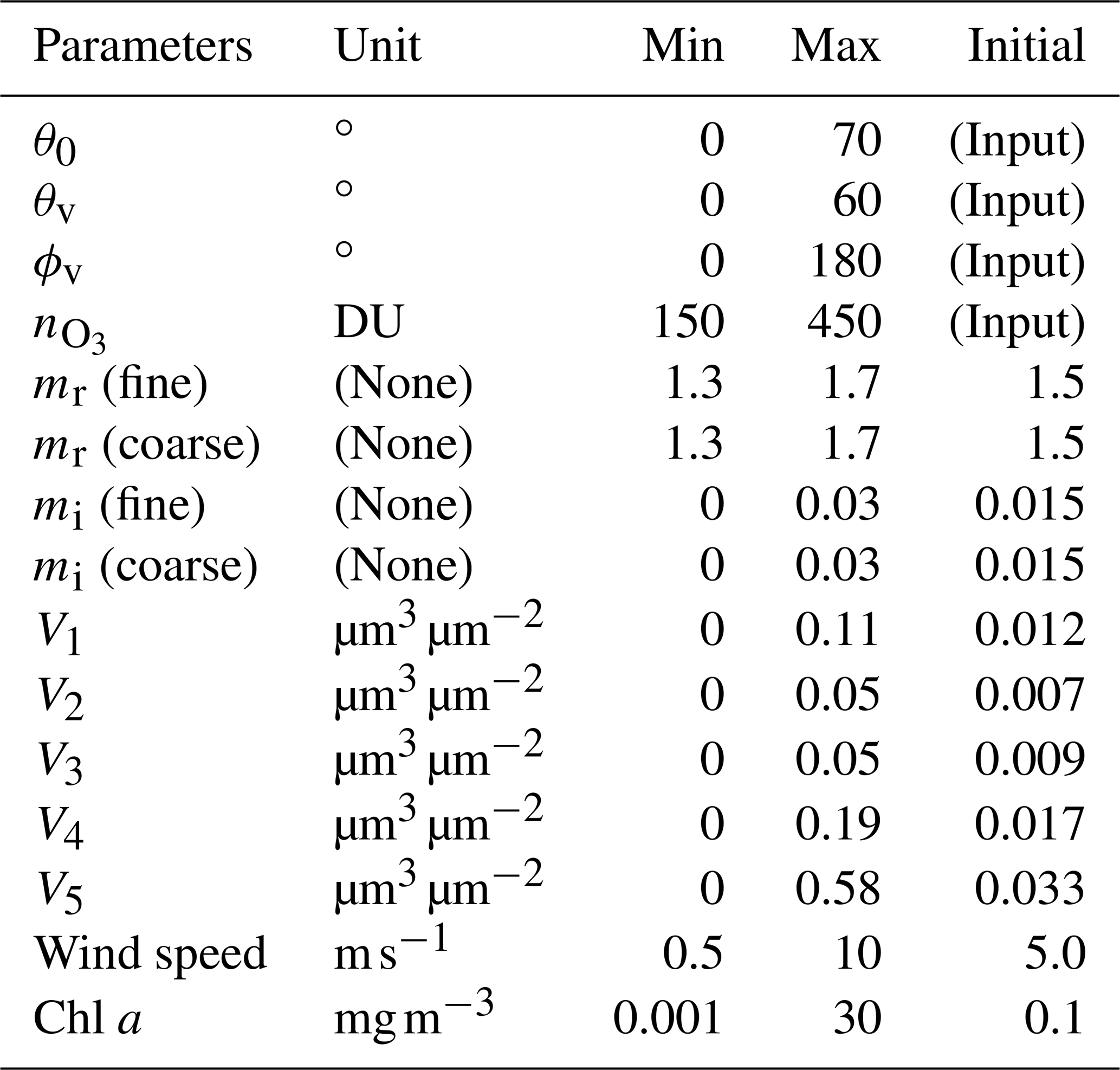
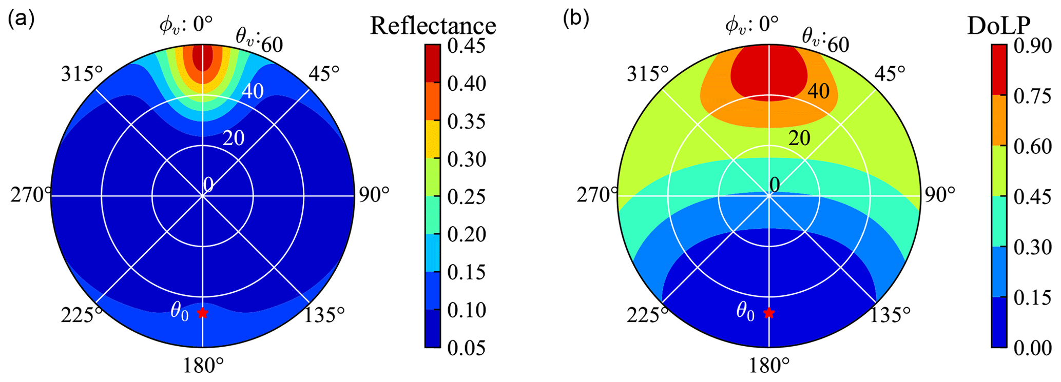
Figure 2The reflectance (a) and DoLP (b) from radiative transfer simulation with the wind speed of 4.13 m s−1, the aerosol optical depth of 0.26, Chl a of 0.05 mg m−3, and ozone column density of 196 DU. The antisolar point is indicated by the red asterisk with a solar zenith angle . θv and ϕv indicate the viewing zenith and relative azimuth angles. The principal plane is defined by the viewing azimuth angle of 0∘ and 180∘.
We randomly selected 20 000 cases out of the total 21 000 simulated cases for the training and validation processes, and the remaining 1000 random cases will be used as test cases to evaluate the NN accuracy, which will be discussed in the next section. To enable the NNs to predict reflectance and DoLP at any given viewing geometry, for each case, we sampled 100 random pairs of viewing zenith and azimuth angles. If the sampled angles fall outside of the predefined angular grids, values from spline interpolation are used. The sunglint angles within an angle of 40∘ to the solar specular reflection direction are removed. Approximately 1 million data points are obtained for each wavelength for training.
To maintain both flexibility and efficiency, we trained two NN models for reflectance and DoLP respectively in the next section. Reflectance and DoLP have different accuracy requirements as discussed in Sect. 2 and also differ in angular variations as shown in the Fig. 2; therefore, it is convenient to control their accuracy through separated training procedures.
3.2 Neural network training
A feed-forward NN can be defined recursively with one input layer, one output layer, and k hidden layers (Aggarwal, 2018):
where x is the input parameter vector including all 15 parameters needed to define the forward model as listed in Table 2. Here x not only contains the retrieval parameters in the state vector defined in Eq. (3) but also includes additional non-retrieval parameters such as the solar zenith angle, viewing zenith and azimuth angles, and the ozone column density. y is a four-dimensional output vector for reflectance or DoLP at the four AirHARP bands. The weight matrix Wp+1 connects the pth and (p+1)th NN layers. The bias vector for the (p+1) layer is defined as bp+1. The output of each layer hp+1 becomes the input of the next layer as shown in Eq. (17). k is the number of hidden layers, and k+1 refers to the output layer. In this study, we tested several NN architectures and eventually chose three hidden layers with the number of nodes of 1024, 256, and 128 as shown in Table 3. The nonlinear activation function Φ used in this model is the Leaky ReLU function, which is defined as
Both Leaky ReLU and ReLU (defined as ) activation functions are simple in their mathematical forms and are tested in our NN trainings. Leaky ReLU is eventually chosen due to its slightly better accuracy achieved than the NN with ReLU.
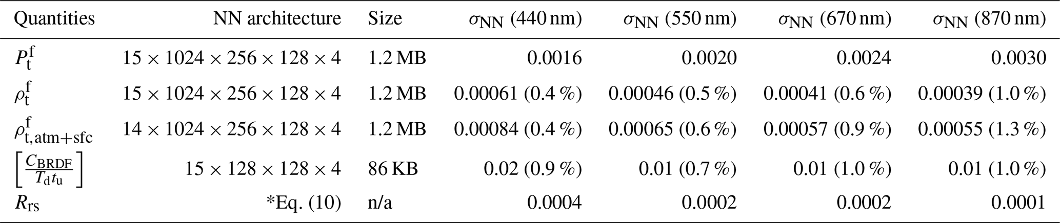
Table 3The accuracy of the NN for the corresponding quantities in terms of the RMSE (σNN) of the difference between the NN-predicted values and the truth values from radiative transfer simulation. The NN architecture denotes the number of the nodes in each layer. The corresponding NN data sizes are indicated. Remote sensing reflectance is computed by Eq. (10) using the NNs for and as discussed in Sect. 3.4. (The percentage values listed below in the parenthesis are the percentage uncertainties defined as the RMSE of the percentage difference between the RT simulation and NN predictions.). n/a means not applicable.
The training process is to minimize the cost function defined as the mean square error between the training data generated from radiative transfer simulations and the NN-predicted values (Aggarwal, 2018). All parameters in the neural network weight matrices and bias vectors, over 670 000 numbers, need to be trained. With this large number of parameters, it is a challenging task to avoid overfitting where the model works well for the training dataset but poorly for the dataset not used in the training process. Several training procedures are performed for reflectance and DoLP data to avoid overfitting and improve NN performance.
-
Both input and output data are normalized before training. We normalize the input data into the range of [0, 1] using the minimum and maximum values from the datasets as listed in Table 2. The reflectance and DoLP in the output layers are normalized by dividing their standard deviation of the training data at each wavelength.
-
The Adam (short for Adaptive Moment Estimation) optimization algorithm (Kingma and Ba, 2015) with weight decay regularization (Loshchilov and Hutter, 2019) is used to update the weights and bias of the NN. The training dataset is divided into multiple mini-batches, each with 1024 random samples. The training iterations loop through all mini-batches in the training data (each loop is called an epoch). Convergence requires training through multiple epochs, where mini-batches are resampled in each epoch.
-
The learning rate determines the step size in the parameter update. We use an exponential decay schedule to reduce the learning rate: we start with a learning rate of 0.005 and reduce the learning rate by a factor of 10 every 200 epochs.
-
To monitor overfitting in the training process, we split the data into 70 % for training and 30 % for validation. We conduct the optimization based on the training dataset, and in the meantime we monitor the performance of training by applying the NN model to the validation dataset. To avoid overfitting, the early-stopping approach is employed where the training is stopped when the cost function on the validation dataset stops to reduce for a threshold of 50 epochs.
The machine-learning Python library PyTorch is used for the training (Paszke et al., 2019). The trained NN model is used to replace the radiative transfer model to compute the reflectance and DoLP in the retrieval algorithm. The Jacobian matrix used in the optimization is computed by the finite difference approximation of the partial derivatives of reflectance and DoLP with respect to the retrieval parameters. Here central difference method is used. Note that the Jacobian matrix can also be computed analytically from the NN model using the automatic differentiation techniques based on the chain rule of differentiation (Baydin et al., 2018). This will be a topic in our future studies.
3.3 Neural network accuracy
After training the NN model, we evaluated its accuracy using synthetic AirHARP measurements generated from the 1000 simulation cases which have not been used in the training and validation process. Each simulation dataset includes polarized reflectance on regular viewing angle grids, which are interpolated to the viewing geometry of AirHARP to create synthetic measurement data and compare with the NN predictions. Glint angles are excluded from the comparison because the NNs are not trained over these angles. As the example shown in Fig. 3, both the reflectance and DoLP are in good agreement between the synthetic data and the NN results, where the maximum absolute differences for reflectance and DoLP are within 0.001 and 0.0025. This translates to a difference for both reflectance and DoLP mostly less than 1 % for bands 440, 550, and 670 nm. The maximum percentage difference can be as large as 3 % for 870 nm bands due to the small reflectance magnitude.

Figure 3The synthetic HARP reflectance (a) and DoLP (b) sampled from the radiative transfer data shown in Fig. 2. Panels (c) and (d) indicate the difference between the NN predictions and RT simulations. Panels (e) and (f) indicate their percentage differences. The positive and negative signs of the viewing zenith angles indicate the azimuth angles of and .

Figure 4Comparison between the radiative transfer simulation and NN prediction: (a, c, e) reflectance (ρ) and (b, d, f) DoLP (P). The scatter plots are shown in panels (a) and (b), the difference in panels (c) and (d), and the percentage difference in panels (e) and (f). For each plot, the data points for the 550, 660, and 870 nm bands are shifted upward by constant offsets consecutively as indicated by the solid cyan lines.
The comparison with all 1000 synthetic datasets and their NN predictions are shown in Fig. 4. The mean absolute error (MAE) and the root mean square error (RMSE) between the simulation data (Ti) and the NN-predicted data (Ri) shown in Fig. 4 are defined as
Both MAE and RMSE are useful metrics, where MAE is less dependent on outliers compared to RMSE.
Analysis shows that the statistics of the differences between the NN prediction and the RT simulations as shown in Fig. 4 can be well modeled by Gaussian distributions and characterized by RMSE. Therefore the RMSE is used to represent the NN uncertainties for both reflectance (σρ,NN) and DoLP (σρ,NN) and will be incorporated into the total uncertainties in the cost function. Table 3 summarizes the uncertainties of the NN models. The σρ,NN at 440 nm is 0.0006, which decreases to 0.0004 at 870 nm. However, due to the smaller reflectance magnitude at 870 nm, the corresponding RMSE for the percentage reflectance difference as shown in Fig. 4 is increased from 0.4 % at 440 nm to 1.0 % at 870 nm. For DoLP, the maximum σP,NN is 0.003 at 870 nm, which decreases to 0.0016 at 440 nm. The uncertainties can be further improved with more training data points. For the readers' information, RMSE of the NN model trained with 20 000 cases (1 million data points) decreases by a factor of in comparison with the one using 10 000 cases (0.5 million data points). It takes 0.01 s in a single-core CPU (AMD EPYC processor) or 1 ms in a GPU (GeForce GTX 1060) to predict all 120 angles for both reflectance and DoLP in the NN forward model. Furthermore, the data sizes for the NNs are minimal, which are 1.2 MB for the reflectance and DoLP and less than 100 KB for the factor (details in Sect. 3.4 as shown in Table 3).
The assessment of the NN accuracy is relative to the synthetic measurements simulated by the vector radiative transfer simulations. To account for the modeling uncertainties of the forward model σf, we consider both the NN accuracy σNN and the numerical accuracy of the radiative transfer simulations σRT for reflectance and DoLP, respectively. Uncertainties due to incomplete assumptions in the forward model are not considered. Several internal parameters determine the numerical accuracy of the radiative transfer simulations. In the framework of the successive order of scattering (Zhai et al., 2008, 2009), these parameters include the number of scattering orders (Ns), the number of Gaussian quadratures for discretizing the viewing zenith angle in the atmosphere (Pa) and ocean (Po), the order of Fourier decomposition (M) for the viewing azimuth angle, and the order of Legendre expansion (L) of the single scattering phase function. In this study, we chose Ns=20, Pa=32, Po=64, M=32, and L=32, which has a higher accuracy than the radiative transfer forward model directly used in our previous retrieval studies (Gao et al., 2020).
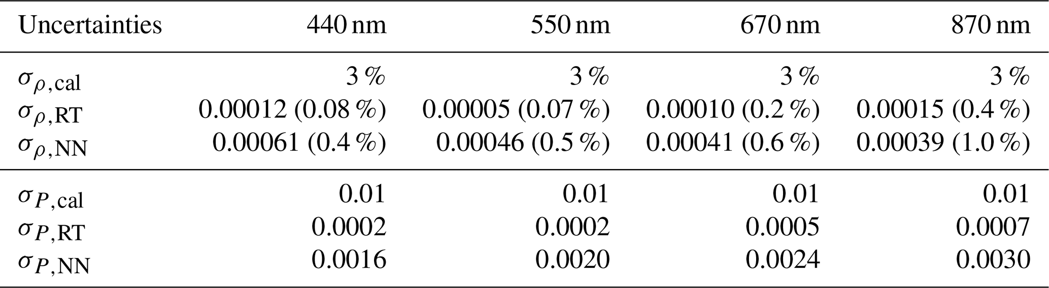
To quantify the accuracy of the radiative transfer calculation used for generating training data (σRT), we simulated an additional 1000 synthetic AirHARP datasets with all internal parameters doubled as the most rigorous calculations, and the viewing angular resolution was reduced from 1∘ to 0.5∘ in order to reduce interpolation errors. The resultant reflectance and DoLP values are compared between these two sets of radiative transfer calculations. The RMSE for each band can be used as a measure of the accuracy for the radiative transfer calculation used to generate the training data (σRT). The uncertainties σRT for reflectance and DoLP are summarized in Table 4, with reflectance uncertainties less than 0.00015 and DoLP uncertainties less than 0.0007 for all AirHARP bands. σρ,RT is about 4 times smaller than the NN uncertainties, and σP,RT is about 4 to 10 times smaller. The measurement uncertainties from calibration (σcal) are also summarized in Table 4. The total forward model uncertainties as in Eq. (7) are much smaller than σcal. The overall uncertainties used in the retrieval cost function in Eq. (3) are dominated by the measurement contributions.
Table 4Comparisons of the uncertainties for reflectance (ρ) and DoLP (P) for both measurement and forward model including calibration uncertainty (σcal), the radiative transfer simulation uncertainty (σRT), and the NN uncertainty (σNN). The same σρ,NN and σP,NN have been shown in Table 3 and are repeated here for comparisons. (As in Table 3, the percentage values listed in the table indicate the percentage uncertainties.)
Furthermore, in this study higher accuracies from the radiative transfer simulations are used for the NN training for comparison with the accuracies from the radiative transfer model directly used in our previous retrieval algorithm. Since the simulations of the training data can be conducted independent of the retrieval algorithm, higher computational costs can be accommodated to improve NN forward model accuracy. After the NN model is trained, the model can be applied to the retrieval algorithm through efficient matrix operations.
3.4 Neural network model for remote sensing reflectance
As discussed in Sect. 2.2, the water-leaving signals are represented by the remote sensing reflectance as defined in Eq. (10) (Mobley et al., 2016). To conduct the atmospheric correction in Eq. (11), we need to determine the reflectance at the aircraft level, transmittance and , and the BRDF correction coefficient CBRDF. Based on Eq. (10), we combined , , and CBRDF into a single term denoted as . To efficiently determine Rrs, two NNs need to be trained to represent , and , respectively.
Following similar NN training schemes as discussed previously, we conducted 10 000 simulations to determine the reflectance at aircraft altitude from a system with only atmosphere and ocean surface (right panel of Fig. 1) and trained the NN for in the same way as . Since this system only includes the atmosphere and ocean surface but without the ocean body, there are a total of 14 input parameters (without Chl a). To train a NN for with , , and CBRDF defined in Eqs. (12)–(14), we obtained five additional quantities corresponding to the abovementioned 10 000 cases with and without ocean body: for the fully coupled system with atmosphere, ocean surface, and ocean body (left panel of Fig. 1), we computed the reflectance just above and below the ocean surface ( and ) and irradiance transmittance just above and below the ocean surface ( and ); for the system without ocean body but with ocean surface (right panel of Fig. 1), we computed the reflectance just above the ocean surface (). The accuracies of the NNs for and are evaluated and shown in Table 3, which has an accuracy around 1 % similar to other quantities.
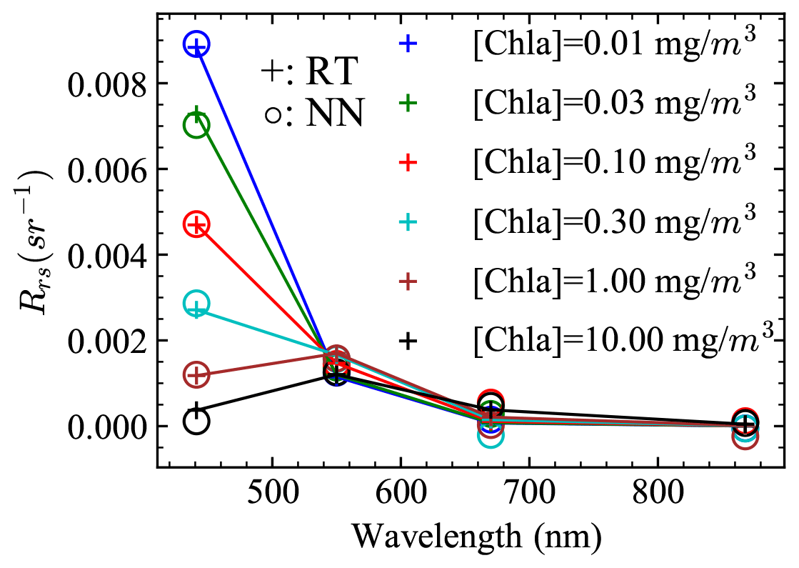
To evaluate the overall accuracy for the Rrs after the BRDF correction, we conducted radiative transfer simulations with a zenith sun and a nadir viewing direction and obtained the truth remote sensing reflectance using the upwelling radiance and downwelling irradiance just above the ocean surface as the examples shown in Fig. 5. The predicted Rrs values were computed from Eq. (10) after the application of two NNs. The RMSEs of the difference between the simulated and NN-predicted Rrs are shown in Table 3, with a maximum value of 0.0004 at wavelength 440 nm and smaller than 0.0002 in other bands.
The NN forward models for reflectance () and DoLP () are used in the FastMAPOL retrieval algorithm as discussed in Sect. 2. To evaluate the performance of the retrieval algorithm, we conducted retrievals on the synthetic AirHARP data. The creation of the synthetic data is discussed in Sect. 3.3. To account for the measurement uncertainties, random noise is added to the simulated data according to the calibration uncertainties as listed in Table 4. The total uncertainties in the cost function include contributions from calibration (σcal), radiative transfer simulation (σRT), and NN model (σNN).
Using the initial values as listed in Table 2, a total of 1000 synthetic AirHARP cases are retrieved with the cost function values (χ2) summarized in Fig. 6. Retrievals with χ2<1.5 are chosen in our following discussion, which includes 96 % of all retrieval cases. Gao et al. (2020) showed that the retrieval results depend on the initial values. Testing with several random sets of initial values shows that the statistics of the retrieval results from the 1000 synthetic cases are robust. As demonstrated by Di Noia et al. (2015) and Di Noia et al. (2017), a better choice of initial values for each pixel in the optimization may further improve the overall retrieval accuracy.
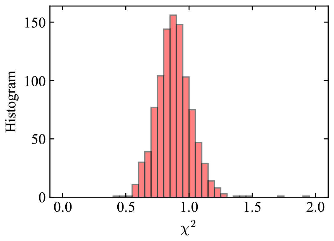
Figure 6Histogram of the cost function values (χ2) with initial values as specified in Table 3 with a total of 1000 cases. The most probable χ2 is 0.82. A threshold of χ2<1.5 is used in the discussion.
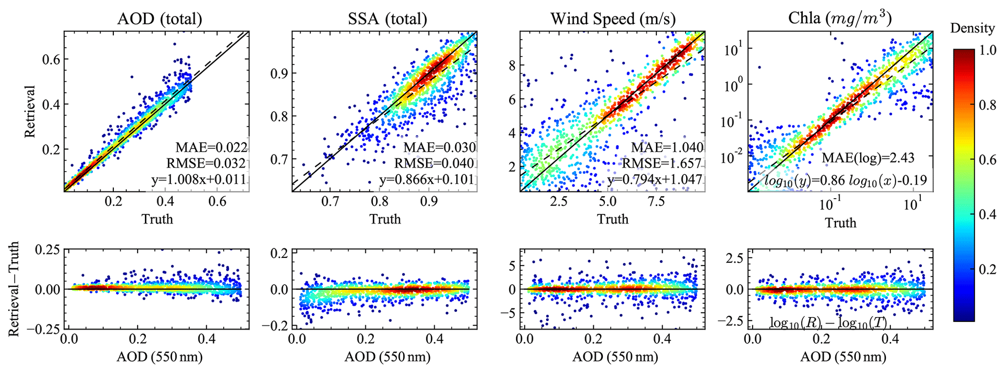
Figure 7The comparisons of the retrieved and truth values for total AOD (550 nm), SSA (550 nm), wind speed, and Chl a are shown in the top panels. The dashed line indicates the linear regression fitting with , where β is the slope and α is the intercept. The lower panels show the difference between the retrieved and truth values of the corresponding upper panel parameters as a function of the total AOD at 550 nm.
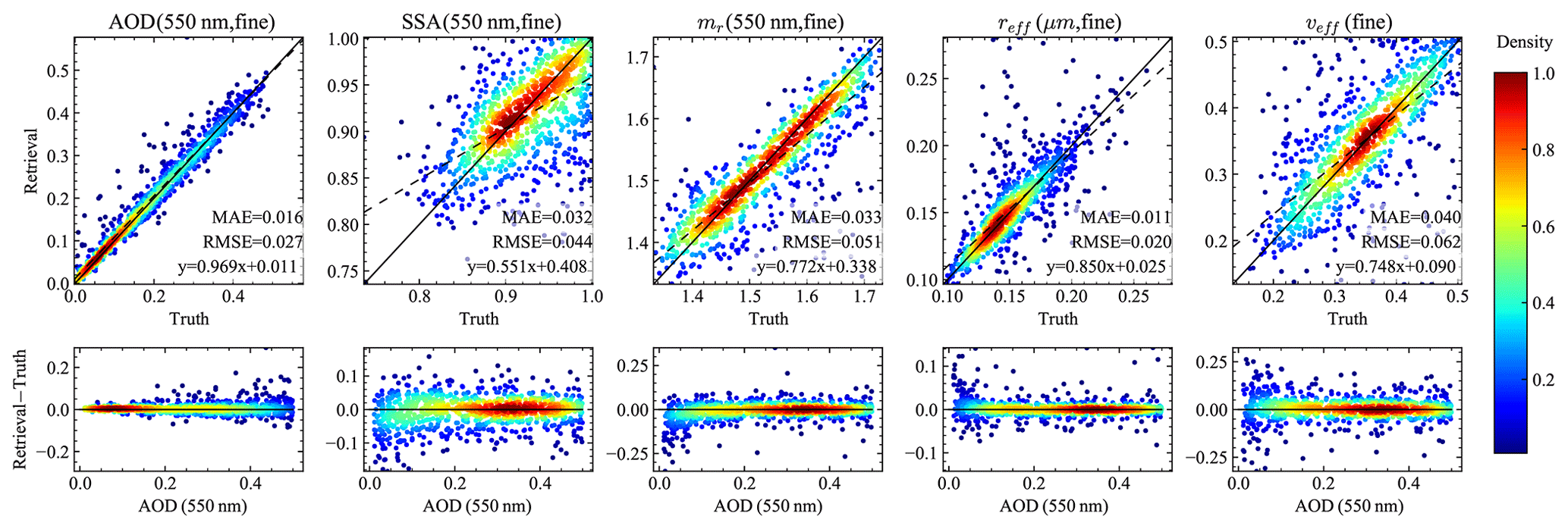
Figure 8The comparisons of the retrieved and truth values for the fine-mode aerosol parameters including AOD, SSA, refractive index (mr), and effective radius (reff) and variance (veff).
With the directly retrieved aerosol refractive index and volume densities (see Table 2) as inputs, the aerosol optical depth (AOD) and single scattering albedo (SSA) for both the fine and coarse modes were computed using additional NNs to represent the Lorenz–Mie calculations in Appendix A. The retrieved total AOD, SSA, wind speed, and Chl a are compared with the truth values as shown in Fig. 7. Total AOD indicates the summation of the fine- and coarse-mode AODs, and total SSA is the ratio of the total scattering and extinction cross sections; both are specified in Appendix A. For fine aerosol, the AOD, SSA, refractive index (mr), and effective radius (reff) and variance (veff) are shown in Fig. 8. The color plots indicate the data point density (normalized by its maximum value) approximated by a kernel density estimation method (Silverman, 1986).

Figure 9The retrieval uncertainties at various aerosol loadings for AOD, SSA, refractive index (mr), effective radius (reff) and variance (veff), wind speed, and Chl a. AOD values at the x axis from 0.1 to 0.5 indicate the five ranges of total AOD including [0.01, 0.1], [0.1, 0.2], [0.2, 0.3], [0.3, 0.4], and [0.4, 0.5], which are used to compute the corresponding uncertainties. Chl a uncertainties are evaluated in terms of MAE in log scale (see Eq. 22), and all other parameters are evaluated in terms of RMSE. AOD (%) indicates the percentage AOD uncertainties comparing to the truth AOD.
In order to quantify the variation of the retrieval uncertainties with respect to different aerosol loadings, we computed the RMSE between the retrieved and truth values at five AOD ranges including [0.01, 0.1], [0.1, 0.2], [0.2, 0.3], [0.3, 0.4], and [0.4, 0.5]. Each AOD range includes approximately 200 cases. Note that as discussed in Sect. 3.3 the total AOD and the fine-mode volume fraction are uniformly sampled for the simulated data; therefore, there is an equal mixing fraction of fine- and coarse-mode aerosol for each AOD range. The retrieval uncertainties for aerosols are shown in Fig. 9, with the corresponding ranges indicated by AOD values from 0.1 to 0.5. All discussions regarding the AOD and SSA are for a wavelength of 550 nm in this section.
As shown in Figs. 7 and 9, the errors of the retrieved total AOD increase with aerosol loadings: the uncertainty (evaluated using RMSE) is 0.008 and 0.015 for the AOD range [0.01, 0.1] and [0.1, 0.2] and increases to 0.035 for the AOD range [0.4, 0.5]. Similar absolute uncertainties are found for both the fine- and coarse-mode AODs, with a slightly smaller value. In percentage, the total AOD uncertainties is 28.3 % at the AOD range [0.01, 0.1], where the large uncertainties are due to the cases with small AODs. For the AOD range from [0.1, 0.2] to [0.4, 0.5], the AOD uncertainties further decrease from 14.4 % to 5.6 %.
Similar to the total AOD uncertainties, the total SSA uncertainties decreases with AOD from 0.05 to 0.02. The fine-mode SSA uncertainties reduce similarly from 0.05 to 0.03. The uncertainties for coarse-mode SSA reduces slightly from 0.1 to 0.08, which is more than twice as large as the fine-mode SSA uncertainties. The uncertainties for the fine-mode mr, reff, and veff show a larger value in the AOD bin of [0.01, 0.1] of 0.06, 0.024 µm, and 0.08 and then remain close to a constant at larger AOD ranges with a smaller value of 0.03, 0.01 µm, and 0.03 respectively. The averaged uncertainties for coarse-mode mr, reff, and veff are approximately 0.08, 0.5 µm, and 0.15 respectively with less AOD dependency at all AOD ranges. The coarse-mode mr uncertainty is more than twice the fine-mode uncertainty. The larger uncertainty values for coarse-mode reff and veff are also related to their large particle size.
For wind speed retrievals as shown in Fig. 7, the agreements between the truth and retrievals depend strongly on the wind speed value itself: when the wind speed is small, there is less retrieval sensitivity due to the removal of glint; for a higher wind speed, the agreements are improved, likely due to the larger range of angles influenced by wind speed. The retrieval uncertainties are shown in Fig. 9; for a wind speed (WS) lower than 3 m s−1, the uncertainty increases from 1.5 to 2.1 m s−1 for AOD ranges from [0.1, 0.2] to [0.4, 0.5]. For wind speed higher than 3 m s−1, the averaged retrieval uncertainty is 1.2 m s−1 with a small variation of less than 0.1 m s−1.
The retrieved and truth Chl a is compared in Fig. 7, where the MAE in log scale is used with the definition
where
where Ri and Ti denote the retrieval and truth values. MAE(log) is recommended by Seegers et al. (2018) as a better metric for Chl a, which indicates the averaged ratio between the retrieval and truth values. The dependency of the MAE(log) for Chl a with the aerosol loadings is shown in Fig. 9. The Chl a retrieval performance depends on the magnitude of the Chl a. In this work, we chose four ranges of Chl a according to the trophic regions discussed in Seegers et al. (2018). Note that Chl a from in situ measurements is typically larger than 0.01 mg m−3, and we chose a broader range of Chl a with its minimum value of 0.001 mg m−3 as listed in Table 2 for sensitivity studies. For and , Chl a retrieval uncertainties vary within 1.3 to 1.6 when AOD < 0.3 and then increase to 2.3 at AOD range [0.4, 0.5]. For and , the uncertainties are generally larger, with a value around 2 to 3.
With the retrieved aerosol and ocean properties, the atmospheric correction procedures can be applied to compute the remote sensing reflectance as discussed in Sect. 3.4. The comparison of the retrieved Rrs with the truth data is shown in Fig. 5. To account for the various solar geometries, the BRDF correction has been applied to the retrieved Rrs as discussed in Sect. 3.4. Note that the factor will not impact the BRDF correction in computing Rrs for the synthetic data, because of the small viewing zenith angles used at the four AirHARP bands, which are 1.22∘, 1.17∘, 0.03∘, and 3.52∘, respectively. The truth Rrs was computed with a zenith sun and a nadir viewing direction, emphasizing the need for the latter correction to the MAP observations. Overall Rrs uncertainties for the four bands are 0.007, 0.0004, 0.0002, and 0.0002 as shown by the RMSE in Fig. 10. MAE showed values of 0.0006, 0.0003, 0.0002, and 0.0001, which are less sensitive to outliers. Note that the atmospheric correction is applied to the synthetic measurements without adding additional random noise in order to evaluate the impacts on Rrs uncertainties from only aerosol and ocean surface property retrievals. The retrieval uncertainties for Rrs for each AirHARP bands are shown in Fig. 10 depending on the aerosol loadings: larger uncertainties are found with larger aerosol optical depth.

Figure 10The difference between the retrieval and truth Rrs with respect to AOD. The truth Rrs is computed with a zenith sun and a nadir viewing direction. The retrieved Rrs follows Eq. (10) with the BRDF correction considered. RMSE and MAE are for all retrievals cases at each wavelength.
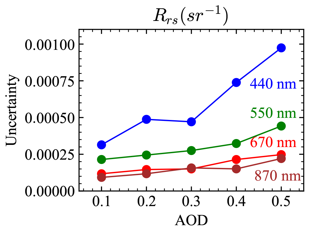
The PACE accuracy requirements on ocean color are specified in terms of the water-leaving reflectance, which can be converted to those of Rrs by dividing them by a factor of π. The resultant requirements in terms of Rrs are 0.0006 sr−1 or 5 % from 400 to 600 nm and 0.0002 sr−1 or 10 % from 600 to 710 nm (Werdell et al., 2019). As shown in Fig. 11, Rrs values at 550 nm are within the requirement of 0.0006 sr−1 for all AOD ranges. For the 440 nm band, when AOD is less than 0.3, the Rrs retrieval uncertainties are less than 0.0005 sr−1, but the uncertainties become as high as 0.001 sr−1 at a larger AOD of 0.5. Rrs at 670 and 870 nm varies in a very small dynamical range and is less impacted by the aerosol retrievals. Rrs uncertainties at 670 and 870 nm are slightly larger than the requirement of 0.0002 sr−1 when AOD (550 nm) is larger than 0.4 and 0.3 respectively. Further work is needed to understand how the uncertainties of the retrieved aerosol properties influence the retrievals. Note that from Table 3, the uncertainties of the Rrs computed using NNs have an uncertainty of 0.0004 to 0.0001 from 440 to 870 nm, which may be further minimized with better training and help to reduce the Rrs retrieval uncertainties.
The ACEPOL field campaign, conducted from October to November of 2017, included a total of six passive and active instruments on the NASA ER-2 high-altitude aircraft (Knobelspiesse et al., 2020) with four MAPs – AirHARP (McBride et al., 2020), AirMSPI (Diner et al., 2013), SPEX airborne (Smit et al., 2019), and the RSP (Cairns et al., 1999) – and two lidars – HSRL-2 (Burton et al., 2015) and CPL (the Cloud Physics Lidar) (McGill et al., 2002). Aerosol retrieval algorithms have been applied for all four MAPs (Fu et al., 2020; Puthukkudy et al., 2020; Gao et al., 2020). The measurement datasets are available from the ACEPOL data portal (Knobelspiesse et al., 2020). In this work, we focus on the study of the AirHARP measurements over ocean scenes as shown in Fig. 12 on 23 October 2017. The viewing angles are within along the track and across the track as shown in the polar plots in Fig. 12. Figure 13 shows the RGB images (670, 550, and 440 nm) for the three scenes at near-nadir viewing direction. AirHARP conducted high-spatial-resolution measurements with a grid size of 55 m and swath width of 42 km at nadir (up to 60 km at far angles). We averaged the reflectance and DoLP respectively within a bin box of 10×10 pixels (550 m×550 m).
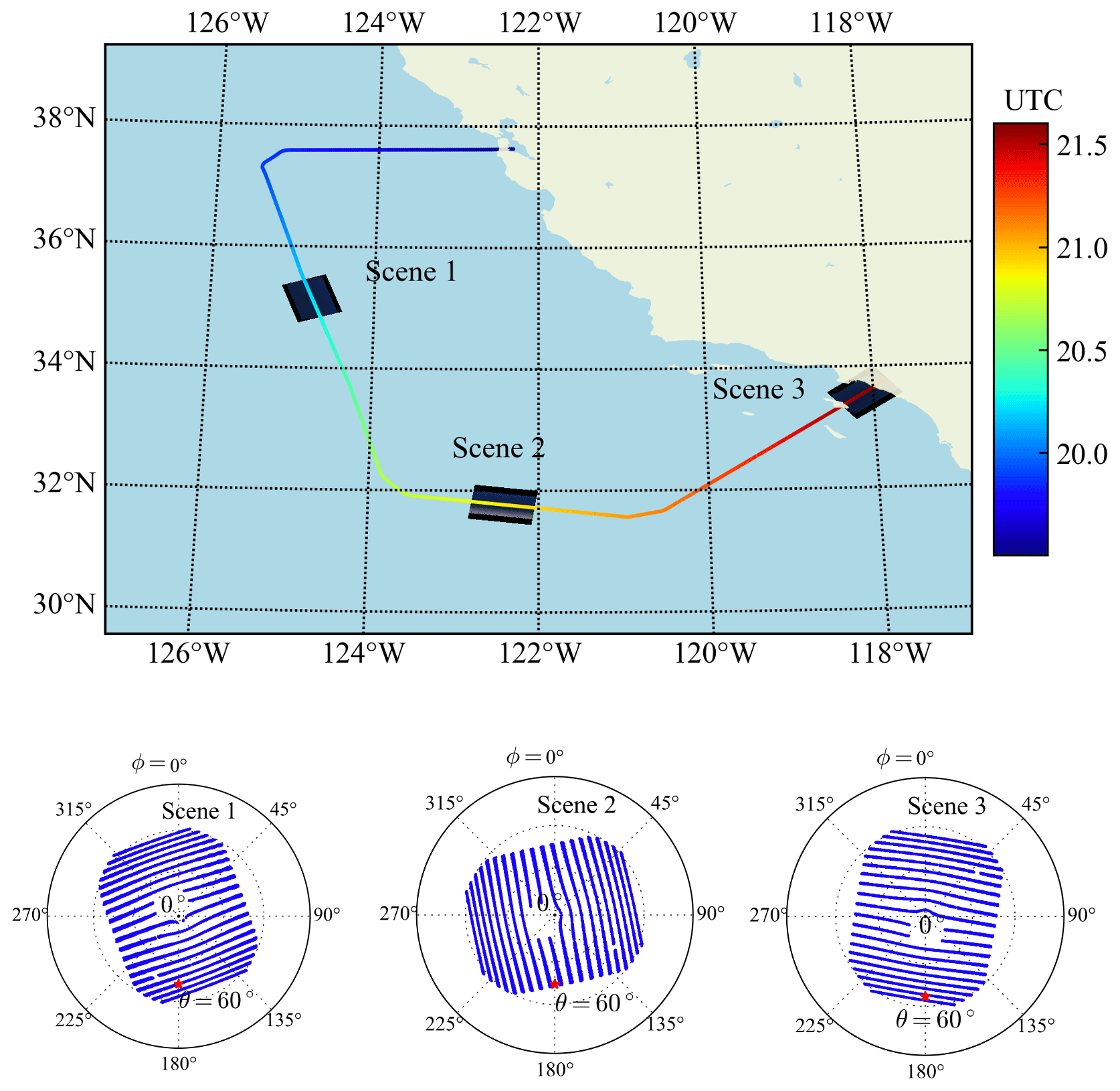
Figure 12The location of the three ocean scenes from AirHARP from ACEPOL on 23 October 2017. The flight track color shows the UTC time along the flight path. The aircraft flew at an altitude of 20.1 km. The viewing zenith and relative azimuth angle (relative to the solar azimuth angle) for the 440 nm band from all pixels in the corresponding scene are shown in the bottom polar plots. The central portion of viewing angle plot is removed due to water condensation on the lens. The averaged solar zenith angles for the three scenes are 47.0∘, 45.6∘, and 52.9∘, respectively, as indicated in the polar plots by the red asterisks.
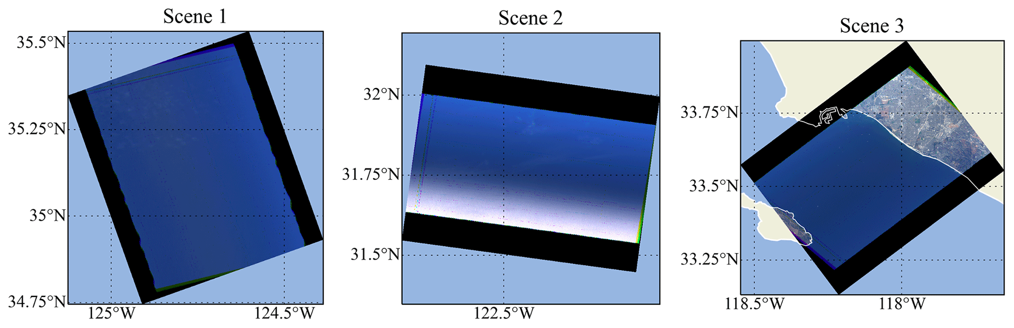
Figure 13The RGB images (670, 550, and 440 nm bands) for the three scenes at near-nadir viewing directions. Scene 1 and Scene 2 observe only ocean, while Scene 3 observes both ocean and land. Sparse thin clouds are visible from Scene 1 and Scene 2. Sunglint can be observed at the lower portion of the Scene 2 image.
The HSRL-2 instrument from ACEPOL provided useful aerosol optical depth ground truth at 355 and 532 nm (Hair et al., 2008; Burton et al., 2016), which was used for the validation of the aerosol retrieval algorithm using the AirHARP data. The HSRL-2 measures the pixels along the track as shown in Fig. 12, where an assumed lidar ratio of 40 sr is multiplied by the aerosol backscatter coefficient derived from the HSRL technique to produce aerosol extinction and AOD at 532 nm. For the low-aerosol-loading cases considered in this study, the assumed lidar ratio approach produces a systematic uncertainty of ±50 % (Fu et al., 2020). In Scene 3, the aircraft also flew over an AERONET USC_SEAPRISM site (33.564∘ N, 118.118∘ W) which is equipped with a CIMEL-based system called the Sea-viewing Wide Field-of-view Sensor (SeaWiFS) Photometer Revision for Incident Surface Measurements (SeaPRISM) that collects radiances at eight wavelengths of 412, 443, 490, 532, 550, 667, 870, and 1020 nm (Zibordi et al., 2009). AOD from the AERONET data product version 3 level 2.0 data was used in this study, which is also consistent with the HSRL-2 AOD at 532 nm as shown latter in Fig. 20. The estimated AERONET AOD uncertainty is from 0.01 to 0.02, with the maximum uncertainty in the UV channels (Giles et al., 2019). We compared AOD from AirHARP retrievals with those from both HSRL and AERONET. Furthermore, to validate the atmospheric correction procedure in the retrieval algorithm, we compared the retrieved remote sensing reflectance with the AERONET ocean color (OC) products as reported by the SeaPRISM measurements at the USC_SEAPRISM site.
Table 5The standard deviations of the reflectance (σρ,avg) and DoLP (σP,avg) are calculated within a 10×10 pixel box and averaged over all angle and pixels from the three scenes (over ocean pixels only). The percentage values listed in the table indicate the percentage uncertainties.

To assess the spatial variability of field measurement, we computed the standard deviations for the reflectance (σρ,avg) and DoLP (σP,avg) within the bin box. Representative values are provided in Table 5. The values of σρ,avg and σP,avg at the 870 nm band are 4.5 % and 0.05, respectively, which suggest larger measurement uncertainties at 870 nm than other bands probably due to small radiometric magnitudes. Meanwhile, our retrieval tests showed larger coarse-mode retrieval uncertainties than synthetic data results. To better constraint retrievals, we assume the coarse-mode aerosol as sea salt by setting its imaginary refractive index to zero. All other retrieval parameter ranges are kept the same as in Table 2. Furthermore, we found our forward model cannot predict the angular variation of DoLP in the 440 nm band well (with an estimated MAE of 0.04), which contributes a major portion to the cost function and increases both fine- and coarse-mode retrieval uncertainties. Therefore, we exclude DoLP in the 440 nm band from our retrievals in this study.
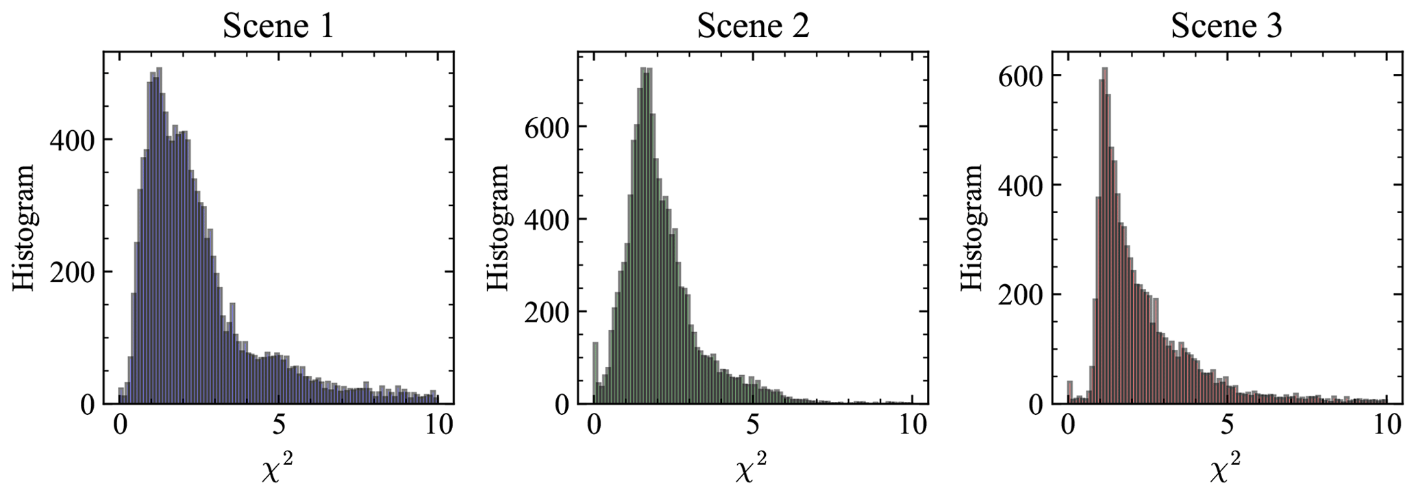
Figure 14The histograms of the cost function values over the three scenes as shown in Fig. 12 with total pixel numbers of 13 491, 13 226, and 9159. Only pixels over ocean are considered.
We conducted retrievals with similar procedures as discussed for synthetic data. The solar and viewing geometries as shown in Fig. 12 and the ozone column density () are assumed to be known inputs to the retrieval algorithm. The averaged values of from MERRA2 over each of the three scenes are obtained, which are 277.5, 278.6, and 281.3 DU respectively. The averaged surface pressures from MERRA2 over the three scenes are 1.008, 1.006 and 1.003 atm, which is consistent with our assumption in the atmosphere model as discussed in Sect. 3. The histograms of χ2 for all pixels retrieved in each scene are shown in Fig. 14. The most probable χ2 values are 1.1, 1.7, and 1.1 respectively.
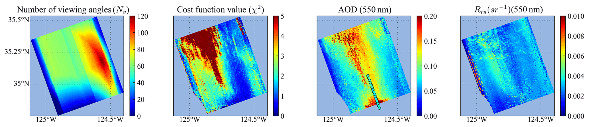
Figure 15The number of viewing angles used in the retrieval (Nv), the cost function value (χ2), the retrieved AOD (550 nm), and Rrs (550 nm) for all pixels in Scene 1. The HSRL AODs at 532 nm are indicated by the colored dots in the AOD plot.
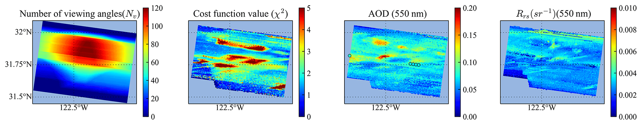
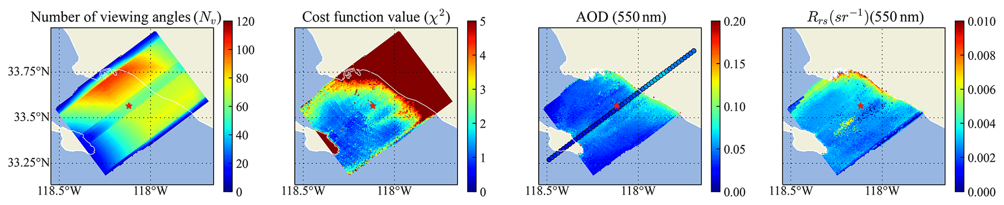
Figure 17Same as Fig. 15 but for Scene 3. The pixels with large χ2 are mostly influenced by the land (upper region) and island (lower left). The retrieved AOD and Rrs over land pixels are not shown. The location of the AERONET USC_SEAPRISM site is indicated by a red star symbol.
To evaluate the retrieval performance, we plotted the map of the total number of viewing angles used in the retrieval (Nv), the cost function χ2, the retrieved AOD (550 nm), and Rrs for each scene in Figs. 15–17. As discussed in Sect. 2, the maximum number of viewing angles is 120 for AirHARP measurements. Figures 15–17 show the number of available viewing angles vary from 0 to 120 due to the removal of glint and other data quality control measures. Discontinuity in the number of angles can be seen as a stripe, due to the removal of angles influenced by water condensation on the lens, which can also be observed in the polar plots in Fig. 12 with the nadir region removed. All three figures show that the number of viewing angles are smaller at the edges parallel to the flight track, where small χ2 can be achieved but may be less reliable.
For pixels with large χ2 as shown in Fig. 14, the forward model cannot fit the measured reflectance or DoLP well, which may be due to cloud contamination (Stap et al., 2015), land, or residuals of glint. In Scene 1, the top region with large χ2 values is impacted by the thin cloud which is visible from Fig. 13. Larger residuals in the 870 nm band between measurement and forward model are also observed. The retrieved AOD are overestimated in this region. In Scene 2, the region with χ2>3 correlates closely with the thin clouds (Fig. 13), which influence nearby AOD and Rrs retrievals. For Scene 3, χ2 become larger than 2 when close to the coast. This may be due to complex water properties which are not well represented by the open-water bio-optical model used in the simulation (Gao et al., 2019). The pixels near the coast are also potentially impacted by the bottom effect and adjacency effect of land pixels.
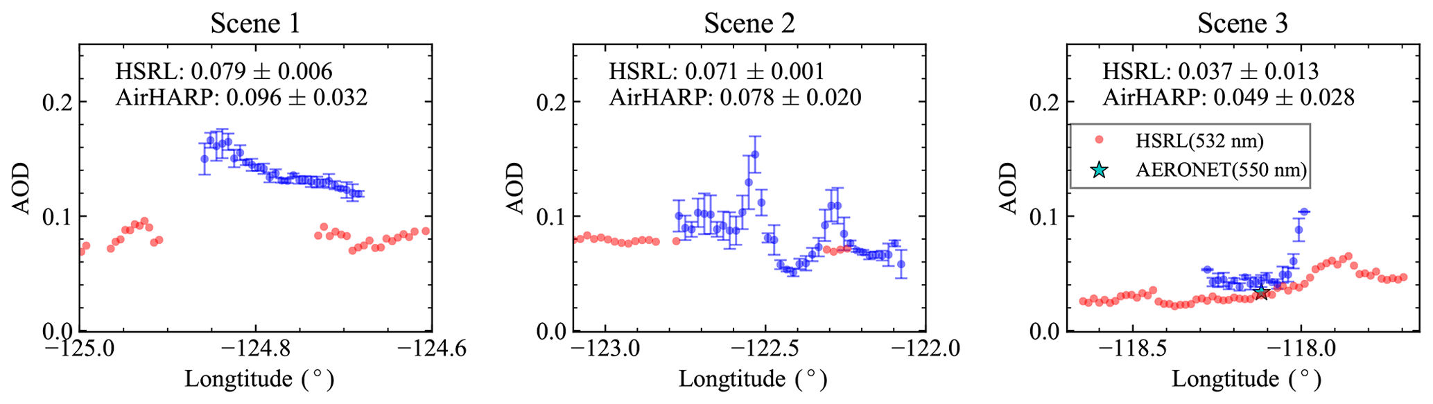
Figure 18Comparison of the retrieved AOD (550 nm) from AirHARP measurement with the AOD (532 nm) from HSRL for Scene 1 to 3. The AOD (550 nm) from the AERONET USC_SeaPRISM site is shown in Scene 3. The AirHARP retrieved AOD is averaged with 4×4 pixels (2.2 km×2.2 km). The averaged AODs and their standard deviations for both AirHARP retrievals and HSRL products are provided in the text. Pixels with Nv>30 and χ2<10 are considered.
To compare with the HSRL AOD in the along-track direction, the retrieved AOD (550 nm) is averaged within a box of 4×4 pixels (2.2 km ×2.2 km). The averaged AOD (550 nm) values and the corresponding standard deviations are shown in Fig. 18. Pixels with Nv>30 and χ2<10 are considered. The overall averaged AODs and their standard deviation are also computed and indicated in the plots. The averaged HSRL AODs are 0.079, 0.071, and 0.037 for Scene 1 to 3. The averaged retrieved AOD (550 nm) are 0.096, 0.078, and 0.049, with relatively larger retrieval variation of 0.02 to 0.03. For Scene 1, most χ2 values are larger than 2, while for the other two scenes, more pixels are less than 2 except for those pixels very close to cloud and coast. In Scene 1, the retrieved AOD is larger than that of the HSRL AOD by 0.03 in the overlapped region, which may be influenced by the remaining effect of water condensation. In Scene 2, the peaks of the retrieved AOD values correspond to the χ2 values larger than 2, which are influenced by the nearby thin cloud. There are no overlapped pixels except the ones associated with high AOD peaks, but the general trend of the retrieved AOD agrees with the HSRL results. For Scene 3, the retrieved AOD values agree well with the HSRL AOD with an average difference of less than 0.01 and χ2 mostly less than 2. However when the pixels are close to the coast, both χ2 and AOD increased significantly as discussed previously.
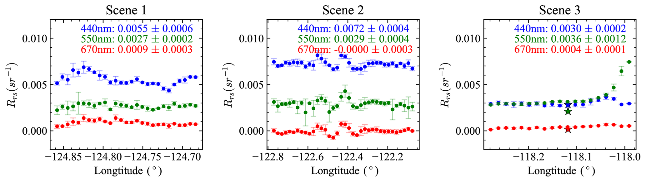
Figure 19Similar to Fig. 18, the retrieved Rrs values are computed for the AirHARP band of 440, 550, and 670 nm bands. The averaged Rrs and its standard deviation are shown in the legends. For Scene 3, Rrs values from the AERONET USC_SeaPRISM site at wavelengths corresponding to AirHARP bands are indicated by the star symbols.
Figure 19 shows the mean value and standard deviation of Rrs averaged in the same way as AOD discussed above. There is similar spatial variation between the retrieved Rrs and AOD. Pixels with large Rrs uncertainties are mostly associated with the large AOD uncertainties shown in Fig. 18. The Rrs values at 440 nm for the three scenes are 0.0055, 0.0072, and 0.0030 sr−1, where the decrease in Rrs from Scene 2 to Scene 3 may be due to the increase in CDOM close to the coast as demonstrated in Fig. 5. Moreover, Rrs values at Scene 1 are likely to be underestimated due to the large χ2 and retrieved AOD over the center of Scene 1. The averaged Rrs values at 550 nm remain approximately constant with a value of 0.0003 sr−1 over all three scenes. Rrs values from the AERONET USC_SeaPRISM site are indicated in Scene 3 of Fig. 19 and also compared in Fig. 20. As discussed in Sect. 2.2, we chose the minimum viewing zenith angle available from the measurements after removing the sunglint. The removal of sunglint improves the Rrs calculation for Scene 2 as shown in Fig. 16. Moreover, we have ignored the factor in Eq. (14), which may cause underestimation of the Rrs at the edge of the image where θv can reach as large as 60∘. However it is challenging to analyze its impact at large θv angles. has a strong dependency on wind speed, but the retrieved wind speeds from current retrievals show large uncertainties. Further work may require a better treatment of sunglint and improved accuracy in wind speed.

Figure 20Comparisons of the AOD and Rrs from AirHARP retrievals with AERONET products. The retrieval results are averaged with 4×4 pixels (2.2 km×2.2 km) around the AERONET USC_SeaPRISM site. This is similar to Figs. 18 and 19, with error bars indicating the standard deviations, but only pixels with χ2<2 are considered. The AERONET AOD and Rrs spectra are taken from 23 October 2017, with the error bars indicating daily variations. HSRL AOD at 532 nm is also shown.
To better compare with AERONET results, we only considered the pixels with χ2<2 and conducted the same averaging (4×4 pixels) around the USC_SeaPRISM site for the retrieved AOD and Rrs. The averaged values and their standard deviations are plotted in Fig. 20. The overall retrieved AOD spectrum is similar to AERONET results with a difference smaller than 0.01. The results are similar to the retrieval results from the Research Scanning Polarimeter as reported by Gao et al. (2020). The retrieved Rrs agrees well with the AERONET Rrs, with a difference of less than 0.001 sr−1. Note that this study is done with a possible AirHARP measurement uncertainty of 3 % in reflectance, which may impact the atmospheric correction accuracy.
The complete retrieval results, including the aerosol microphysical properties, wind speed, Chl a, and atmospheric-correction-related datasets, are provided in the “Data availability” section. The retrieval uncertainties for aerosol microphysical properties are relatively large due to the small aerosol optical depths. Chl a retrievals are sensitive to the aerosol retrievals and are more challenging to retrieve accurately at small values as discussed in Sect. 4.
The NN model greatly improved the speed of the forward model used in the iterative optimization approach and boosted the efficiency of the FastMAPOL retrievals. The average retrieval speed for one pixel with FastMAPOL is approximately 3 s with a single CPU core, or approximately 0.3 s with a GPU using the same hardware as mentioned in Sect. 3.3. Comparing to the retrieval speed of approximately 1 h per pixel using conventional radiative transfer forward model, the computational acceleration is 103 times faster with CPU or 104 times with GPU processors. Meanwhile, the NN model maintains a high accuracy as shown in Tables 3 and 4. For retrieval algorithms running the radiative transfer simulation, the accuracy is often tuned down to reduce the simulation time. By training a NN, however, the high accuracy of the radiative transfer model simulation can be achieved, as has been demonstrated in this work. Thus, despite the one-time high computational costs in generating the training datasets and conducting the training, the trained NN can be applied efficiently to large observational datasets in the retrieval algorithm.
In the retrieval of the AirHARP field measurement, each pixel has multiple viewing angles that are aggregated from measurements at different times with slightly different solar zenith angles. The NN used in FastMAPOL computes the polarimetric measurement for specific solar zenith angles for each viewing direction, and, therefore, the variation of the solar zenith angle can be captured. These effects may be small for AirHARP measurement in ACEPOL, with a maximum solar zenith angle difference within 0.6∘. However, this capability can help to minimize the impacts of the solar angle for HARP2 in spaceborne measurements, which can reach to a maximum difference of 1.5∘ for HARP2 observations.
With the efficient retrievals from FastMAPOL, we have discussed the retrieval performance and uncertainties for the aerosol properties, including AOD, SSA, refractive index, and particle sizes. Since the AirHARP measurements share many similar characteristics with HARP2 as planned for the PACE mission, the knowledge from the retrieval analysis can help to understand the retrieval performance for the HARP2 instrument in spaceborne measurements. Note that HARP2 is likely to have higher accuracy due to the onboard calibration capability and the potential to conduct cross calibration with the OCI instrument. For the development of the NN forward model for spaceborne measurements, similar training procedures can be applied with the sensor altitude at the top of the atmosphere instead of the aircraft altitude used in this study. Due to the impact of retrieval capability by geometry (Fougnie et al., 2020), solar and viewing geometries according to the PACE orbits need to be considered.
The water-leaving reflectance is obtained from the atmospheric correction process using the aerosol and ocean properties retrieved from the AirHARP measurements, and a similar procedure can be applied to future HARP2 retrievals. Since the hyperspectral OCI in PACE will provide high-accuracy measurements, the retrieved information can be applied to OCI and therefore assist hyperspectral atmosphere corrections as demonstrated by Gao et al. (2020) and Hannadige et al. (2021). However, aerosol retrieval and atmospheric correction are challenging in the UV spectral range (Remer et al., 2019a). For the ocean bio-optical model in this study, the water properties are modeled as open-ocean waters parameterized by a single Chl a value. For complex coastal water, complex bio-optical models are preferred in the retrieval of both accurate aerosol properties and water-leaving signals as demonstrated by Gao et al. (2019).
We have demonstrated the application of a NN for highly accurate forward model calculations of polarimetric measurements for AirHARP. Additional NN models were used to conduct atmospheric correction. These models are used in the FastMAPOL joint retrieval algorithm to conduct simultaneous aerosol property and water-leaving signal retrieval. Applications to both the synthetic AirHARP data and field measurements from ACEPOL are discussed. The uncertainties of the retrieved aerosol properties and remote sensing reflectance are discussed for different aerosol loadings. These results from AirHARP retrievals can help to evaluate the retrieval capabilities for the HARP2 instrument on PACE. In the application to field measurements from ACEPOL, the impacts of the number of viewing angles and the value of cost function to the retrieval quality are discussed. Further comparison with the HSRL and AERONET OC data shows good performance in the retrieval of AOD and remote sensing reflectance. Furthermore, the NN forward model and the associated retrieval algorithm enable fast and practical retrievals of the polarimetric measurement, thus making the algorithm practical for analysis of large data volumes expected from spaceborne imagers such as HARP2. The experience and methodology can be used to help the algorithm development of other satellite instruments in polarimetric remote sensing.
As summarized in Table 3, we have discussed the NNs used to represent the total reflectance () and DoLP (), which are then used as the forward model in the retrieval algorithm. Using the retrieved aerosol parameters, NNs for and are used to compute remote sensing reflectance. To expedite and simplify the calculation of aerosol single scattering properties such as AOD and SSA as discussed in Sect. 4, we developed four additional NNs to represent the AOD and SSA for both fine and coarse modes, respectively. These NNs are only used to analyze the retrieved aerosol properties and are not used in the retrieval process. The NN architectures and accuracy are shown in Table A1. The input parameters for the fine-mode SSA and AOD are the three submode volume densities and the real and imaginary parts of refractive index, with a total of five parameter. For coarse-mode aerosols, there are a total of four parameters with only two submodes used. The outputs are the AOD and SSA at the four AirHARP bands.
A total of 10 000 training data points are generated in the same way as in Sect. 3.1 using the Lorenz–Mie code discussed in Sect. 2. The NN model accuracy is evaluated with an additional 1000 data points not used in the training. As shown in Table A1, the accuracy is much smaller than the retrieval uncertainties shown in Fig. 9; therefore, the NNs for AOD and SSA provide sufficient accuracy to evaluate the aerosol single scattering properties.
Table A1The accuracy of the NN for the corresponding quantities in terms of the RMSE (σ) between the NN-predicted values and the truth values from the Lorenz–Mie calculations.
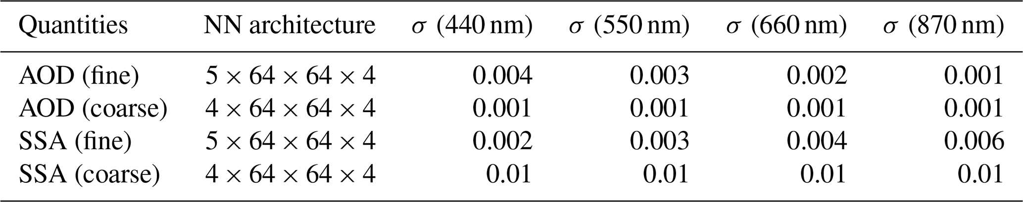
With the fine- and coarse-mode AOD and SSA evaluated, the total AOD and SSA can be derived. The total AOD (τt) is the summation of the fine- and coarse-mode AODs as
where τf and τc are the fine- and coarse-mode AODs. The total (or averaged) SSA (ωt) is defined as the ratio of the total scattering cross section and the total extinction cross section for both fine and coarse modes, which can be computed as
where ωf and ωc are the fine- and coarse-mode SSA.
The data files for AirHARP and HSRL-2 used in this study are available from the ACEPOL website (https://doi.org/10.5067/SUBORBITAL/ACEPOL2017/DATA001, ACEPOL Science Team, 2017). Complete retrieval results as well as data related to atmospheric correction from the three AirHARP scenes discussed in Sect. 5 are available from NASA Open Data Portal: https://data.nasa.gov/Earth-Science/FastMAPOL_ACEPOL_AIRHARP_L2/8b9y-7rgh (Gao, 2021).
MG, BAF, KK, and PWZ formulated the original concept for this study. MG developed the NN model and generated the scientific data. PWZ developed the radiative transfer code. KK, PWZ, BC, OH, and YH advised on the uncertainty model and retrieval algorithm. BAF, AI, and PJW advised on the atmospheric correction. KK, AI, and YH advised on the NN model. JG supported the parallel computing of the training data. VM, XX, BM, and AP provided and advised on the AirHARP data. RF and SB provided and advised on the HSRL-2 data. All authors participated in reviewing and editing this paper.
The authors declare that they have no conflict of interest.
The authors would like to thank the ACEPOL science team for conducting the field campaign and providing the data, as well as the AERONET principal investigators and their teams for establishing and operating the USC_SEAPRISM site. We thank the NASA Ocean Biology Processing Group (OBPG) system team for support in high-performance computing (HPC) and the NASA Advanced Software Technologies Group (ASTG) for Python and machine-learning trainings. We appreciate the constructive discussions with Frederick Patt, Andy Sayer, and George Kattawar, as well as the valuable comments from Yingxi Shi and Reed Espinosa.
Meng Gao, Bryan A. Franz, Kirk Knobelspiesse, Brian Cairns, Amir Ibrahim, Joel Gales, and P. Jeremy Werdell have been supported by the NASA PACE project. Peng-Wang Zhai has been supported by NASA (grants 80NSSC18K0345 and 80NSSC20M0227). Funding for the ACEPOL field campaign came from NASA (ACE and CALIPSO missions) and SRON. Part of this work has been funded by the NWO/NSO project ACEPOL (project no. ALW-GO/16-09). The ACEPOL campaign has been supported by the Radiation Sciences Program.
This research has been supported by the NASA PACE project, NASA (grant nos. 80NSSC18K0345 and 80NSSC20M0227), NASA (ACE and CALIPSO missions), SRON, NWO/NSO project ACEPOL (project no. ALW-GO/16-09), and the Radiation Sciences Program.
This paper was edited by Alexander Kokhanovsky and reviewed by Yingxi Shi and Reed Espinosa.
ACEPOL Science Team: Aerosol Characterization from Polarimeter and Lidar Campaign, NASA Langley Atmospheric Science Data Center DAAC, https://doi.org/10.5067/SUBORBITAL/ACEPOL2017/DATA001, 2017. a
Aggarwal, C. C.: Neural Networks and Deep Learning: A Textbook, Springer, Cham, Switzerland, 2018. a, b
Anderson, G., Clough, S., Kneizys, F., Chetwynd, J., and Shettle, E.: AFGL Atmospheric Constituent Profiles (0.120 km), Air Force Geophysics Lab., Hanscom AFB, MA, USA, 1986. a
Baydin, A. G., Pearlmutter, B. A., Radul, A. A., and Siskind, J. M.: Automatic differentiation in machine learning: a survey, J. Mach. Learn. Res., 18, 1–43, 2018. a
Bogumil, K., Orphal, J., Homann, T., Voigt, S., Spietz, P., Fleischmann, O., Vogel, A., Hartmann, M., Kromminga, H., Bovensmann, H., Frerick, J., and Burrows, J.: Measurements of molecular absorption spectra with the SCIAMACHY pre-flight model: instrument characterization and reference data for atmospheric remote-sensing in the 230–2380 nm region, J. Photoch. Photobio. A, 157, 167–184, https://doi.org/10.1016/S1010-6030(03)00062-5, 2003. a
Boucher, O., Randall, D., Artaxo, P., Bretherton, C., Feingold, G., Forster, P., Kerminen, V.-M., Kondo, Y., Liao, H., Lohmann, U., Rasch, P., Satheesh, S., Sherwood, S., Stevens, B., and Zhang, X.: Clouds and Aerosols, in: Climate Change 2013: The Physical Science Basis. Contribution of Working Group Ito the Fifth Assessment Report of the Intergovernmental Panel on Climate Change, edited by: Stocker, T. F., Qin, D., Plattner, G.-K., Tignor, M., Allen, S. K., Boschung, J., Nauels, A., Xia, Y., Bex, V., and Midgley, P. M., Cambridge University Press, Cambridge, UK and New York, NY, USA, 571–658, https://doi.org/10.1017/CBO9781107415324.016, 2013. a, b
Branch, M. A., Coleman, T. F., and Li, Y.: A Subspace, Interior, and Conjugate Gradient Method for Large-Scale Bound-Constrained Minimization Problems, SIAM J. Sci. Comput., 21, 1–23, https://doi.org/10.1137/S1064827595289108, 1999. a
Buehler, S. A., Eriksson, P., Kuhn, T., von Engeln, A., and Verdes, C.: ARTS, the atmospheric radiative transfer simulator, J. Quant. Spectrosc. Ra., 91, 65–93, 2005. a
Burton, S. P., Hair, J. W., Kahnert, M., Ferrare, R. A., Hostetler, C. A., Cook, A. L., Harper, D. B., Berkoff, T. A., Seaman, S. T., Collins, J. E., Fenn, M. A., and Rogers, R. R.: Observations of the spectral dependence of linear particle depolarization ratio of aerosols using NASA Langley airborne High Spectral Resolution Lidar, Atmos. Chem. Phys., 15, 13453–13473, https://doi.org/10.5194/acp-15-13453-2015, 2015. a
Burton, S. P., Chemyakin, E., Liu, X., Knobelspiesse, K., Stamnes, S., Sawamura, P., Moore, R. H., Hostetler, C. A., and Ferrare, R. A.: Information content and sensitivity of the 3β+2α lidar measurement system for aerosol microphysical retrievals, Atmos. Meas. Tech., 9, 5555–5574, https://doi.org/10.5194/amt-9-5555-2016, 2016. a
Cairns, B., Russell, E. E., and Travis, L. D.: Research Scanning Polarimeter: calibration and ground-based measurements, Proc. SPIE, 3754, 186–196, https://doi.org/10.1117/12.366329, 1999. a
Chen, C., Dubovik, O., Fuertes, D., Litvinov, P., Lapyonok, T., Lopatin, A., Ducos, F., Derimian, Y., Herman, M., Tanré, D., Remer, L. A., Lyapustin, A., Sayer, A. M., Levy, R. C., Hsu, N. C., Descloitres, J., Li, L., Torres, B., Karol, Y., Herrera, M., Herreras, M., Aspetsberger, M., Wanzenboeck, M., Bindreiter, L., Marth, D., Hangler, A., and Federspiel, C.: Validation of GRASP algorithm product from POLDER/PARASOL data and assessment of multi-angular polarimetry potential for aerosol monitoring, Earth Syst. Sci. Data, 12, 3573–3620, https://doi.org/10.5194/essd-12-3573-2020, 2020. a
Chowdhary, J., Cairns, B., Mishchenko, M., and Travis, L.: Retrieval of aerosol properties over the ocean using multispectral and multiangle Photopolarimetric measurements from the Research Scanning Polarimeter, Geophys. Res. Lett., 28, 243–246, https://doi.org/10.1029/2000GL011783, 2001. a
Chowdhary, J., Cairns, B., Mishchenko, M. I., Hobbs, P. V., Cota, G. F., Redemann, J., Rutledge, K., Holben, B. N., and Russell, E.: Retrieval of Aerosol Scattering and Absorption Properties from Photopolarimetric Observations over the Ocean during the CLAMS Experiment, J. Atmos. Sci., 62, 1093–1117, https://doi.org/10.1175/JAS3389.1, 2005. a
d'Almeida, G. A., Koepke, P., and Shettle, E. P.: Atmospheric aerosols: global climatology and radiative characteristics, A. Deepak Pub., Hampton, Va., USA, 1991. a
Di Noia, A., Hasekamp, O. P., van Harten, G., Rietjens, J. H. H., Smit, J. M., Snik, F., Henzing, J. S., de Boer, J., Keller, C. U., and Volten, H.: Use of neural networks in ground-based aerosol retrievals from multi-angle spectropolarimetric observations, Atmos. Meas. Tech., 8, 281–299, https://doi.org/10.5194/amt-8-281-2015, 2015. a, b
Di Noia, A., Hasekamp, O. P., Wu, L., van Diedenhoven, B., Cairns, B., and Yorks, J. E.: Combined neural network/Phillips–Tikhonov approach to aerosol retrievals over land from the NASA Research Scanning Polarimeter, Atmos. Meas. Tech., 10, 4235–4252, https://doi.org/10.5194/amt-10-4235-2017, 2017. a, b
Dierssen, H. M. and Randolph, K.: Remote Sensing of Ocean Color, Springer, New York, NY, 439–472, https://doi.org/10.1007/978-1-4614-5684-1_18, 2013. a
Diner, D. J., Xu, F., Garay, M. J., Martonchik, J. V., Rheingans, B. E., Geier, S., Davis, A., Hancock, B. R., Jovanovic, V. M., Bull, M. A., Capraro, K., Chipman, R. A., and McClain, S. C.: The Airborne Multiangle SpectroPolarimetric Imager (AirMSPI): a new tool for aerosol and cloud remote sensing, Atmos. Meas. Tech., 6, 2007–2025, https://doi.org/10.5194/amt-6-2007-2013, 2013. a
Diner, D. J., Boland, S. W., Brauer, M., Bruegge, C., Burke, K. A., Chipman, R., Girolamo, L. D., Garay, M. J., Hasheminassab, S., Hyer, E., Jerrett, M., Jovanovic, V., Kalashnikova, O. V., Liu, Y., Lyapustin, A. I., Martin, R. V., Nastan, A., Ostro, B. D., Ritz, B., Schwartz, J., Wang, J., and Xu, F.: Advances in multiangle satellite remote sensing of speciated airborne particulate matter and association with adverse health effects: from MISR to MAIA, J. Appl. Remote Sens., 12, 1–22, https://doi.org/10.1117/1.JRS.12.042603, 2018. a
Dubovik, O., Sinyuk, A., Lapyonok, T., Holben, B. N., Mishchenko, M., Yang, P., Eck, T. F., Volten, H., Muñoz, O., Veihelmann, B., van der Zande, W. J., Leon, J.-F., Sorokin, M., and Slutsker, I.: Application of spheroid models to account for aerosol particle nonsphericity in remote sensing of desert dust, J. Geophys. Res.-Atmos., 111, D11208, https://doi.org/10.1029/2005JD006619, 2006. a, b
Dubovik, O., Herman, M., Holdak, A., Lapyonok, T., Tanré, D., Deuzé, J. L., Ducos, F., Sinyuk, A., and Lopatin, A.: Statistically optimized inversion algorithm for enhanced retrieval of aerosol properties from spectral multi-angle polarimetric satellite observations, Atmos. Meas. Tech., 4, 975–1018, https://doi.org/10.5194/amt-4-975-2011, 2011. a
Dubovik, O., Lapyonok, T., Litvinov, P., Herman, M., Fuertes, D., Ducos, F., Lopatin, A., Chaikovsky, A., Torres, B., Derimian, Y., Huang, X., Aspetsberger, M., and Federspiel, C.: GRASP: a versatile algorithm for characterizing the atmosphere, SPIE Newsroom, https://doi.org/10.1117/2.1201408.005558, 2014. a
Dubovik, O., Li, Z., Mishchenko, M. I., Tanré, D., Karol, Y., Bojkov, B., Cairns, B., Diner, D. J., Espinosa, W. R., Goloub, P., Gu, X., Hasekamp, O., Hong, J., Hou, W., Knobelspiesse, K. D., Landgraf, J., Li, L., Litvinov, P., Liu, Y., Lopatin, A., Marbach, T., Maring, H., Martins, V., Meijer, Y., Milinevsky, G., Mukai, S., Parol, F., Qiao, Y., Remer, L., Rietjens, J., Sano, I., Stammes, P., Stamnes, S., Sun, X., Tabary, P., Travis, L. D., Waquet, F., Xu, F., Yan, C., and Yin, D.: Polarimetric remote sensing of atmospheric aerosols: Instruments, methodologies, results, and perspectives, J. Quant. Spectrosc. Ra., 224, 474–511, https://doi.org/10.1016/j.jqsrt.2018.11.024, 2019. a
Fan, C., Fu, G., Di Noia, A., Smit, M., H. H. Rietjens, J., A. Ferrare, R., Burton, S., Li, Z., and P. Hasekamp, O.: Use of A Neural Network-Based Ocean Body Radiative Transfer Model for Aerosol Retrievals from Multi-Angle Polarimetric Measurements, Remote Sens.-Basel, 11, 2877, https://doi.org/10.3390/rs11232877, 2019. a, b, c
Fan, Y., Li, W., Gatebe, C. K., Jamet, C., Zibordi, G., Schroeder, T., and Stamnes, K.: Atmospheric correction over coastal waters using multilayer neural networks, Remote Sens. Environ., 199, 218–240, https://doi.org/10.1016/j.rse.2017.07.016, 2017. a, b
Fougnie, B., Marbach, T., Lacan, A., Lang, R., Schlüssel, P., Poli, G., Munro, R., and Couto, A. B.: The multi-viewing multi-channel multi-polarisation imager – Overview of the 3MI polarimetric mission for aerosol and cloud characterization, J. Quant. Spectrosc. Ra., 219, 23–32, https://doi.org/10.1016/j.jqsrt.2018.07.008, 2018. a
Fougnie, B., Chimot, J., Vázquez-Navarro, M., Marbach, T., and Bojkov, B.: Aerosol retrieval from space – how does geometry of acquisition impact our ability to characterize aerosol properties, J. Quant. Spectrosc. Ra., 256, 107304, https://doi.org/10.1016/j.jqsrt.2020.107304, 2020. a
Frouin, R. J., Franz, B. A., Ibrahim, A., Knobelspiesse, K., Ahmad, Z., Cairns, B., Chowdhary, J., Dierssen, H. M., Tan, J., Dubovik, O., Huang, X., Davis, A. B., Kalashnikova, O., Thompson, D. R., Remer, L. A., Boss, E., Coddington, O., Deschamps, P.-Y., Gao, B.-C., Gross, L., Hasekamp, O., Omar, A., Pelletier, B., Ramon, D., Steinmetz, F., and Zhai, P.-W.: Atmospheric Correction of Satellite Ocean-Color Imagery During the PACE Era, Front. Earth Sci., 7, 145, https://doi.org/10.3389/feart.2019.00145, 2019. a
Fu, G. and Hasekamp, O.: Retrieval of aerosol microphysical and optical properties over land using a multimode approach, Atmos. Meas. Tech., 11, 6627–6650, https://doi.org/10.5194/amt-11-6627-2018, 2018. a
Fu, G., Hasekamp, O., Rietjens, J., Smit, M., Di Noia, A., Cairns, B., Wasilewski, A., Diner, D., Seidel, F., Xu, F., Knobelspiesse, K., Gao, M., da Silva, A., Burton, S., Hostetler, C., Hair, J., and Ferrare, R.: Aerosol retrievals from different polarimeters during the ACEPOL campaign using a common retrieval algorithm, Atmos. Meas. Tech., 13, 553–573, https://doi.org/10.5194/amt-13-553-2020, 2020. a, b, c
Gao, M.: FastMAPOL AirHARP Level 2 data product, available at: https://data.nasa.gov/Earth-Science/FastMAPOL_ACEPOL_AIRHARP_L2/8b9y-7rgh, last access: 26 May 2021. a
Gao, M., Zhai, P.-W., Franz, B., Hu, Y., Knobelspiesse, K., Werdell, P. J., Ibrahim, A., Xu, F., and Cairns, B.: Retrieval of aerosol properties and water-leaving reflectance from multi-angular polarimetric measurements over coastal waters, Opt. Express, 26, 8968–8989, https://doi.org/10.1364/OE.26.008968, 2018. a, b, c, d
Gao, M., Zhai, P.-W., Franz, B. A., Hu, Y., Knobelspiesse, K., Werdell, P. J., Ibrahim, A., Cairns, B., and Chase, A.: Inversion of multiangular polarimetric measurements over open and coastal ocean waters: a joint retrieval algorithm for aerosol and water-leaving radiance properties, Atmos. Meas. Tech., 12, 3921–3941, https://doi.org/10.5194/amt-12-3921-2019, 2019. a, b, c, d, e, f, g, h, i, j
Gao, M., Zhai, P.-W., Franz, B. A., Knobelspiesse, K., Ibrahim, A., Cairns, B., Craig, S. E., Fu, G., Hasekamp, O., Hu, Y., and Werdell, P. J.: Inversion of multiangular polarimetric measurements from the ACEPOL campaign: an application of improving aerosol property and hyperspectral ocean color retrievals, Atmos. Meas. Tech., 13, 3939–3956, https://doi.org/10.5194/amt-13-3939-2020, 2020. a, b, c, d, e, f, g, h, i, j, k, l, m
Gelaro, R., McCarty, W., Suárez, M. J., Todling, R., Molod, A., Takacs, L., Randles, C. A., Darmenov, A., Bosilovich, M. G., Reichle, R., Wargan, K., Coy, L., Cullather, R., Draper, C., Akella, S., Buchard, V., Conaty, A., da Silva, A. M., Gu, W., Kim, G.-K., Koster, R., Lucchesi, R., Merkova, D., Nielsen, J. E., Partyka, G., Pawson, S., Putman, W., Rienecker, M., Schubert, S. D., Sienkiewicz, M., and Zhao, B.: The Modern-Era Retrospective Analysis for Research and Applications, Version 2 (MERRA-2), J. Climate, 30, 5419–5454, https://doi.org/10.1175/JCLI-D-16-0758.1, 2017. a
Giles, D. M., Sinyuk, A., Sorokin, M. G., Schafer, J. S., Smirnov, A., Slutsker, I., Eck, T. F., Holben, B. N., Lewis, J. R., Campbell, J. R., Welton, E. J., Korkin, S. V., and Lyapustin, A. I.: Advancements in the Aerosol Robotic Network (AERONET) Version 3 database – automated near-real-time quality control algorithm with improved cloud screening for Sun photometer aerosol optical depth (AOD) measurements, Atmos. Meas. Tech., 12, 169–209, https://doi.org/10.5194/amt-12-169-2019, 2019. a
Goodfellow, I., Bengio, Y., and Courville, A.: Deep Learning, MIT Press, Cambridge, Massachusetts, USA, 2016. a, b
Gordon, I., Rothman, L., Hill, C., Kochanov, R., Tan, Y., Bernath, P., Birk, M., Boudon, V., Campargue, A., Chance, K., Drouin, B., Flaud, J.-M., Gamache, R., Hodges, J., Jacquemart, D., Perevalov, V., Perrin, A., Shine, K., Smith, M.-A., Tennyson, J., Toon, G., Tran, H., Tyuterev, V., Barbe, A., Császár, A., Devi, V., Furtenbacher, T., Harrison, J., Hartmann, J.-M., Jolly, A., Johnson, T., Karman, T., Kleiner, I., Kyuberis, A., Loos, J., Lyulin, O., Massie, S., Mikhailenko, S., Moazzen-Ahmadi, N., Müller, H., Naumenko, O., Nikitin, A., Polyansky, O., Rey, M., Rotger, M., Sharpe, S., Sung, K., Starikova, E., Tashkun, S., Auwera, J. V., Wagner, G., Wilzewski, J., Wcisło, P., Yu, S., and Zak, E.: The HITRAN2016 molecular spectroscopic database, J. Quant. Spectrosc. Ra., 203, 3–69, https://doi.org/10.1016/j.jqsrt.2017.06.038, 2017. a
Gorshelev, V., Serdyuchenko, A., Weber, M., Chehade, W., and Burrows, J. P.: High spectral resolution ozone absorption cross-sections – Part 1: Measurements, data analysis and comparison with previous measurements around 293 K, Atmos. Meas. Tech., 7, 609–624, https://doi.org/10.5194/amt-7-609-2014, 2014. a
Hair, J. W., Hostetler, C. A., Cook, A. L., Harper, D. B., Ferrare, R. A., Mack, T. L., Welch, W., Izquierdo, L. R., and Hovis, F. E.: Airborne High Spectral Resolution Lidar for profiling aerosol optical properties, Appl. Optics, 47, 6734–6752, https://doi.org/10.1364/AO.47.006734, 2008. a, b
Hannadige, N. K., Zhai, P.-W., Gao, M., Franz, B. A., Hu, Y., Knobelspiesse, K., Werdell, P. J., Ibrahim, A., Cairns, B., and Hasekamp, O. P.: Atmospheric correction over the ocean for hyperspectral radiometers using multi-angle polarimetric retrievals, Opt. Express, 29, 4504–4522, https://doi.org/10.1364/OE.408467, 2021. a, b
Hansen, J. E. and Travis, L. D.: Light scattering in planetary atmospheres, Space Sci. Rev., 16, 527–610, https://doi.org/10.1007/BF00168069, 1974. a
Hasekamp, O. P. and Landgraf, J.: Retrieval of aerosol properties over land surfaces: capabilities of multiple-viewing-angle intensity and polarization measurements, Appl. Optics, 46, 3332–3344, https://doi.org/10.1364/AO.46.003332, 2007. a
Hasekamp, O. P., Litvinov, P., and Butz, A.: Aerosol properties over the ocean from PARASOL multiangle photopolarimetric measurements, J. Geophys. Res.-Oceans, 116, D14204, https://doi.org/10.1029/2010JD015469, 2011. a
Hasekamp, O. P., Fu, G., Rusli, S. P., Wu, L., Noia, A. D., aan de Brugh, J., Landgraf, J., Smit, J. M., Rietjens, J., and van Amerongen, A.: Aerosol measurements by SPEXone on the NASA PACE mission: expected retrieval capabilities, J. Quant. Spectrosc. Ra., 227, 170–184, https://doi.org/10.1016/j.jqsrt.2019.02.006, 2019a. a
Hasekamp, O. P., Gryspeerdt, E., and Quaas, J.: Analysis of polarimetric satellite measurements suggests stronger cooling due to aerosol-cloud interactions, Nat. Commun., 10, 5405, https://doi.org/10.1038/s41467-019-13372-2, 2019b. a
Holben, B., Eck, T., Slutsker, I., Tanré, D., Buis, J., Setzer, A., Vermote, E., Reagan, J., Kaufman, Y., Nakajima, T., Lavenu, F., Jankowiak, I., and Smirnov, A.: AERONET – A Federated Instrument Network and Data Archive for Aerosol Characterization, Remote Sens. Environ., 66, 1–16, https://doi.org/10.1016/S0034-4257(98)00031-5, 1998. a
Kawata, Y.: Circular polarization of sunlight reflected by planetary atmospheres, Icarus, 33, 217–232, https://doi.org/10.1016/0019-1035(78)90035-0, 1978. a
Kingma, D. P. and Ba, J.: Adam: A Method for Stochastic Optimization, 3rd International Conference for Learning Representations, 7–9 May 2015, San Diego, USA, 2015. a
Knobelspiesse, K., Cairns, B., Mishchenko, M., Chowdhary, J., Tsigaridis, K., van Diedenhoven, B., Martin, W., Ottaviani, M., and Alexandrov, M.: Analysis of fine-mode aerosol retrieval capabilities by different passive remote sensing instrument designs, Optics Express, 20, 21457–21484, https://doi.org/10.1364/OE.20.021457, 2012. a, b
Knobelspiesse, K., Barbosa, H. M. J., Bradley, C., Bruegge, C., Cairns, B., Chen, G., Chowdhary, J., Cook, A., Di Noia, A., van Diedenhoven, B., Diner, D. J., Ferrare, R., Fu, G., Gao, M., Garay, M., Hair, J., Harper, D., van Harten, G., Hasekamp, O., Helmlinger, M., Hostetler, C., Kalashnikova, O., Kupchock, A., Longo De Freitas, K., Maring, H., Martins, J. V., McBride, B., McGill, M., Norlin, K., Puthukkudy, A., Rheingans, B., Rietjens, J., Seidel, F. C., da Silva, A., Smit, M., Stamnes, S., Tan, Q., Val, S., Wasilewski, A., Xu, F., Xu, X., and Yorks, J.: The Aerosol Characterization from Polarimeter and Lidar (ACEPOL) airborne field campaign, Earth Syst. Sci. Data, 12, 2183–2208, https://doi.org/10.5194/essd-12-2183-2020, 2020. a, b, c
Li, L., Dubovik, O., Derimian, Y., Schuster, G. L., Lapyonok, T., Litvinov, P., Ducos, F., Fuertes, D., Chen, C., Li, Z., Lopatin, A., Torres, B., and Che, H.: Retrieval of aerosol components directly from satellite and ground-based measurements, Atmos. Chem. Phys., 19, 13409–13443, https://doi.org/10.5194/acp-19-13409-2019, 2019. a
Li, Z., Guo, J., Ding, A., Liao, H., Liu, J., Sun, Y., Wang, T., Xue, H., Zhang, H., and Zhu, B.: Aerosol and boundary-layer interactions and impact on air quality, Natl. Sci. Rev., 4, 810–833, https://doi.org/10.1093/nsr/nwx117, 2017. a
Li, Z., Hou, W., Hong, J., Zheng, F., Luo, D., Wang, J., Gu, X., and Qiao, Y.: Directional Polarimetric Camera (DPC): Monitoring aerosol spectral optical properties over land from satellite observation, J. Quant. Spectrosc. Ra., 218, 21–37, https://doi.org/10.1016/j.jqsrt.2018.07.003, 2018. a
Lin, H. W., Tegmark, M., and Rolnick, D.: Why Does Deep and Cheap Learning Work So Well?, J. Stat. Phys., 168, 1223–1247, https://doi.org/10.1007/s10955-017-1836-5, 2017. a
Loshchilov, I. and Hutter, F.: Decoupled Weight Decay Regularization, International Conference on Learning Representations, 6–9 May 2019, New Orleans, USA, 2019. a
Martins, J. V., Fernandez-Borda, R., McBride, B., Remer, L., and Barbosa, H. M. J.: The HARP hyperangular imaging polarimeter and the need for small satellite payloads with high science payoff for earth science remote sensing, in: IGARSS 2018 – 2018 IEEE International Geoscience and Remote Sensing Symposium, 22–27 July 2018, Valencia, Spain, 6304–6307, https://doi.org/10.1109/IGARSS.2018.8518823, 2018. a
McBride, B. A., Martins, J., Puthukuddy, A., Xu, X., Borda, R. F., Barbosa, H. M. J., Hasekamp, O., and Remer, L. A.: The Hyper-Angular Rainbow Polarimeter-2 (HARP-2): A wide FOV polarimetric imager for high resolution spatial and angular characterization of cloud and aerosol microphysics, in: Proceedings of the 70th International Astronautical Congress, 21–25 October 2019, Washington D.C., USA, IAC–19–B1.2.7, 2019. a
McBride, B. A., Martins, J. V., Barbosa, H. M. J., Birmingham, W., and Remer, L. A.: Spatial distribution of cloud droplet size properties from Airborne Hyper-Angular Rainbow Polarimeter (AirHARP) measurements, Atmos. Meas. Tech., 13, 1777–1796, https://doi.org/10.5194/amt-13-1777-2020, 2020. a, b
McGill, M., Hlavka, D., Hart, W., Scott, V. S., Spinhirne, J., and Schmid, B.: Cloud Physics Lidar: instrument description and initial measurement results, Appl. Optics, 41, 3725–3734, https://doi.org/10.1364/AO.41.003725, 2002. a
Mishchenko, M. I. and Travis, L. D.: Satellite retrieval of aerosol properties over the ocean using polarization as well as intensity of reflected sunlight, J. Geophys. Res.-Atmos., 102, 16989–17013, https://doi.org/10.1029/96JD02425, 1997. a
Mishchenko, M. I., Travis, L. D., and Lacis, A. A.: Scattering, Absorption, and Emission of Light by Small Particles, Cambridge University Press, Cambridge, UK, 2002. a
Mobley, C. D., Werdell, J., Franz, B., Ahmad, Z., and Bailey, S.: Atmospheric Correction for Satellite Ocean Color Radiometry, National Aeronautics and Space Administration, Washington, D.C., USA, 2016. a, b, c, d
Moré, J. J.: The Levenberg-Marquardt algorithm: Implementation and theory, in: Numerical Analysis, edited by: Watson, G. A., Springer, Berlin, Heidelberg, 105–116, 1978. a
Morel, A. and Gentili, B.: Diffuse reflectance of oceanic waters. II I. Implication of bidirectionality for the remote-sensing problem, Appl. Optics, 35, 4850–4862, https://doi.org/10.1364/AO.35.004850, 1996. a
Morel, A., Antoine, D., and Gentili, B.: Bidirectional reflectance of oceanic waters: accounting for Raman emission and varying particle scattering phase function, Appl. Optics, 41, 6289–6306, https://doi.org/10.1364/AO.41.006289, 2002. a, b, c
Mukherjee, L., Zhai, P.-W., Gao, M., Hu, Y., A. Franz, B., and Werdell, P. J.: Neural Network Reflectance Prediction Model for Both Open Ocean and Coastal Waters, Remote Sens.-Basel, 12, 1421, https://doi.org/10.3390/rs12091421, 2020. a
Paszke, A., Gross, S., Massa, F., Lerer, A., Bradbury, J., Chanan, G., Killeen, T., Lin, Z., Gimelshein, N., Antiga, L., Desmaison, A., Kopf, A., Yang, E., DeVito, Z., Raison, M., Tejani, A., Chilamkurthy, S., Steiner, B., Fang, L., Bai, J., and Chintala, S.: PyTorch: An Imperative Style, High-Performance Deep Learning Library, in: Advances in Neural Information Processing Systems, 32, 8024–8035, available at: http://papers.neurips.cc/paper/9015-pytorch-an-imperative-style-high-performance-deep-learning-library.pdf (last access: 26 May 2021), 2019. a
Plankton, Aerosol, Cloud, ocean Ecosystem (PACE) mission: The PACE Level 1C data format, available at: https://oceancolor.gsfc.nasa.gov/data/pace/PACE_L1C_Format_DRAFTv20200918.pdf (last access: 26 May 2021), 2020. a
Platt, T., Hoepffner, N., Stuart, V., and Brown, C.: Why Ocean Colour? The Societal Benefits of Ocean-Colour Technology, International Ocean Colour Coordinating Group (IOCCG), Dartmouth, Nova Scotia, Canada, 2008. a
Puthukkudy, A., Martins, J. V., Remer, L. A., Xu, X., Dubovik, O., Litvinov, P., McBride, B., Burton, S., and Barbosa, H. M. J.: Retrieval of aerosol properties from Airborne Hyper-Angular Rainbow Polarimeter (AirHARP) observations during ACEPOL 2017, Atmos. Meas. Tech., 13, 5207–5236, https://doi.org/10.5194/amt-13-5207-2020, 2020. a, b, c, d
Remer, L. A., Davis, A. B., Mattoo, S., Levy, R. C., Kalashnikova, O. V., Coddington, O., Chowdhary, J., Knobelspiesse, K., Xu, X., Ahmad, Z., Boss, E., Cairns, B., Dierssen, H. M., Diner, D. J., Franz, B., Frouin, R., Gao, B.-C., Ibrahim, A., Martins, J. V., Omar, A. H., Torres, O., Xu, F., and Zhai, P.-W.: Retrieving Aerosol Characteristics From the PACE Mission, Part 1: Ocean Color Instrument, Front. Earth Sci., 7, 152, https://doi.org/10.3389/feart.2019.00152, 2019a. a, b
Remer, L. A., Knobelspiesse, K., Zhai, P.-W., Xu, F., Kalashnikova, O. V., Chowdhary, J., Hasekamp, O., Dubovik, O., Wu, L., Ahmad, Z., Boss, E., Cairns, B., Coddington, O., Davis, A. B., Dierssen, H. M., Diner, D. J., Franz, B., Frouin, R., Gao, B.-C., Ibrahim, A., Levy, R. C., Martins, J. V., Omar, A. H., and Torres, O.: Retrieving Aerosol Characteristics From the PACE Mission, Part 2: Multi-Angle and Polarimetry, Front. Environ. Sci., 7, 94, https://doi.org/10.3389/fenvs.2019.00094, 2019b. a
Rietjens, J., Campo, J., Chanumolu, A., Smit, M., Nalla, R., Fernandez, C., Dingjan, J., van Amerongen, A., and Hasekamp, O.: Expected performance and error analysis for SPEXone, a multi-angle channeled spectropolarimeter for the NASA PACE mission, in: Polarization Science and Remote Sensing IX, edited by: Craven, J. M., Shaw, J. A., and Snik, F., vol. 11132, International Society for Optics and Photonics, SPIE, 34–47, https://doi.org/10.1117/12.2530729, 2019. a
Rogers, C.: Inverse Methods for Atmospheric Sounding:Theory and Practice, World Scientific World Scientific Publishing, Singapore, 2000. a
Seegers, B. N., Stumpf, R. P., Schaeffer, B. A., Loftin, K. A., and Werdell, P. J.: Performance metrics for the assessment of satellite data products: an ocean color case study, Opt. Express, 26, 7404–7422, https://doi.org/10.1364/OE.26.007404, 2018. a, b
Serdyuchenko, A., Gorshelev, V., Weber, M., Chehade, W., and Burrows, J. P.: High spectral resolution ozone absorption cross-sections – Part 2: Temperature dependence, Atmos. Meas. Tech., 7, 625–636, https://doi.org/10.5194/amt-7-625-2014, 2014. a
Shettle, E. P. and Fenn, R. W.: Models for the aerosols of the lower atmosphere and the effects of humidity variations on their optical properties, Environmental Research Papers, Air Force Geophysics Lab., Hanscom AFB, MA. Optical Physics Div, 1979. a
Shi, C., Hashimoto, M., Shiomi, K., and Nakajima, T.: Development of an Algorithm to Retrieve AerosolOptical Properties Over Water Using an ArtificialNeural Network Radiative Transfer Scheme: First Result From GOSAT-2/CAI-2, IEEE T. Geosci. Remote, https://doi.org/10.1109/TGRS.2020.3038892, online first, 2020. a, b
Shiraiwa, M., Ueda, K., Pozzer, A., Lammel, G., Kampf, C. J., Fushimi, A., Enami, S., Arangio, A. M., Fröhlich-Nowoisky, J., Fujitani, Y., Furuyama, A., Lakey, P. S. J., Lelieveld, J., Lucas, K., Morino, Y., Pöschl, U., Takahama, S., Takami, A., Tong, H., Weber, B., Yoshino, A., and Sato, K.: Aerosol Health Effects from Molecular to Global Scales, Environ. Sci. Technol., 51, 13545–13567, https://doi.org/10.1021/acs.est.7b04417, 2017. a
Silverman, B.: Density Estimation for Statistics and Data Analysis, Monographs on Statistics and Applied Probability, vol. 26, Chapman and Hall, London, UK, 1986. a
Smit, J. M., Rietjens, J. H. H., van Harten, G., Noia, A. D., Laauwen, W., Rheingans, B. E., Diner, D. J., Cairns, B., Wasilewski, A., Knobelspiesse, K. D., Ferrare, R., and Hasekamp, O. P.: SPEX airborne spectropolarimeter calibration and performance, Appl. Optics, 58, 5695–5719, https://doi.org/10.1364/AO.58.005695, 2019. a
Stamnes, S., Hostetler, C., Ferrare, R., Burton, S., Liu, X., Hair, J., Hu, Y., Wasilewski, A., Martin, W., van Diedenhoven, B., Chowdhary, J., Cetinić, I., Berg, L. K., Stamnes, K., and Cairns, B.: Simultaneous polarimeter retrievals of microphysical aerosol and ocean color parameters from the “MAPP” algorithm with comparison to high-spectral-resolution lidar aerosol and ocean products, Appl. Optics, 57, 2394–2413, https://doi.org/10.1364/AO.57.002394, 2018. a
Stap, F. A., Hasekamp, O. P., and Röckmann, T.: Sensitivity of PARASOL multi-angle photopolarimetric aerosol retrievals to cloud contamination, Atmos. Meas. Tech., 8, 1287–1301, https://doi.org/10.5194/amt-8-1287-2015, 2015. a
Tanré, D., Bréon, F. M., Deuzé, J. L., Dubovik, O., Ducos, F., François, P., Goloub, P., Herman, M., Lifermann, A., and Waquet, F.: Remote sensing of aerosols by using polarized, directional and spectral measurements within the A-Train: the PARASOL mission, Atmos. Meas. Tech., 4, 1383–1395, https://doi.org/10.5194/amt-4-1383-2011, 2011. a
UMBC Earth and Space Institute: HARP CubeSat, available at: https://esi.umbc.edu/hyper-angular-rainbow-polarimeter/, last access: 25 May 2021. a
Virtanen, P., Gommers, R., Oliphant, T. E., Haberland, M., Reddy, T., Cournapeau, D., Burovski, E., Peterson, P., Weckesser, W., Bright, J., van der Walt, S. J., Brett, M., Wilson, J., Millman, K. J., Mayorov, N., Nelson, A. R. J., Jones, E., Kern, R., Larson, E., Carey, C. J., Polat, İ., Feng, Y., Moore, E. W., VanderPlas, J., Laxalde, D., Perktold, J., Cimrman, R., Henriksen, I., Quintero, E. A., Harris, C. R., Archibald, A. M., Ribeiro, A. H., Pedregosa, F., van Mulbregt, P., and SciPy 1.0 Contributors: SciPy 1.0: Fundamental Algorithms for Scientific Computing in Python, Nat. Methods, 17, 261–272, https://doi.org/10.1038/s41592-019-0686-2, 2020. a
Wang, J., Xu, X., Ding, S., Zeng, J., Spurr, R., Liu, X., Chance, K., and Mishchenko, M.: A numerical testbed for remote sensing of aerosols, and its demonstration for evaluating retrieval synergy from a geostationary satellite constellation of GEO-CAPE and GOES-R, J. Quant. Spectrosc. Ra., 146, 510–528, https://doi.org/10.1016/j.jqsrt.2014.03.020, 2014. a
Werdell, P. J., Behrenfeld, M. J., Bontempi, P. S., Boss, E., Cairns, B., Davis, G. T., Franz, B. A., Gliese, U. B., Gorman, E. T., Hasekamp, O., Knobelspiesse, K. D., Mannino, A., Martins, J. V., McClain, C. R., Meister, G., and Remer, L. A.: The Plankton, Aerosol, Cloud, Ocean Ecosystem Mission: Status, Science, Advances, B. Am. Meteorol. Soc., 100, 1775–1794, https://doi.org/10.1175/BAMS-D-18-0056.1, 2019. a, b
Westberry, T., Shi, Y., Yu, H., Behrenfeld, M., and Remer, L.: Satellite-Detected Ocean Ecosystem Response to Volcanic Eruptions in the Subarctic Northeast Pacific Ocean, Geophys. Res. Lett., 46, 11270–11280, https://doi.org/10.1029/2019GL083977, 2019. a
Wu, L., Hasekamp, O., van Diedenhoven, B., and Cairns, B.: Aerosol retrieval from multiangle, multispectral photopolarimetric measurements: importance of spectral range and angular resolution, Atmos. Meas. Tech., 8, 2625–2638, https://doi.org/10.5194/amt-8-2625-2015, 2015. a, b
Xu, F., Dubovik, O., Zhai, P.-W., Diner, D. J., Kalashnikova, O. V., Seidel, F. C., Litvinov, P., Bovchaliuk, A., Garay, M. J., van Harten, G., and Davis, A. B.: Joint retrieval of aerosol and water-leaving radiance from multispectral, multiangular and polarimetric measurements over ocean, Atmos. Meas. Tech., 9, 2877–2907, https://doi.org/10.5194/amt-9-2877-2016, 2016. a, b
Xu, F., Diner, D. J., Dubovik, O., and Schechner, Y.: A Correlated Multi-Pixel Inversion Approach for Aerosol Remote Sensing, Remote Sens.-Basel, 11, 746, https://doi.org/10.3390/rs11070746, 2019. a
Zhai, P.-W., Kattawar, G. W., and Yang, P.: Impulse response solution to the three-dimensional vector radiative transfer equation in atmosphere-ocean systems. I. Monte Carlo method, Appl. Optics, 47, 1037–1047, 2008. a
Zhai, P.-W., Hu, Y., Trepte, C. R., and Lucker, P. L.: A vector radiative transfer model for coupled atmosphere and ocean systems based on successive order of scattering method, Opt. Express, 17, 2057–2079, 2009. a, b, c, d
Zhai, P.-W., Hu, Y., Chowdhary, J., Trepte, C. R., Lucker, P. L., and Josset, D. B.: A vector radiative transfer model for coupled atmosphere and ocean systems with a rough interface, J. Quant. Spectrosc. Ra., 111, 1025–1040, 2010. a, b, c
Zhai, P.-W., Boss, E., Franz, B., Werdell, P. J., and Hu, Y.: Radiative Transfer Modeling of Phytoplankton Fluorescence Quenching Processes, Remote Sens.-Basel, 10, 1309, https://doi.org/10.3390/rs10081309, 2018. a
Zibordi, G., Mélin, F., Berthon, J.-F., Holben, B., Slutsker, I., Giles, D., D'Alimonte, D., Vandemark, D., Feng, H., Schuster, G., Fabbri, B. E., Kaitala, S., and Seppälä, J.: AERONET-OC: A Network for the Validation of Ocean Color Primary Products, J. Atmos. Ocean. Tech., 26, 1634–1651, https://doi.org/10.1175/2009JTECHO654.1, 2009. a
- Abstract
- Introduction
- Joint aerosol and ocean color retrieval algorithm
- Neural network for forward model
- Joint retrieval results on synthetic AirHARP measurements
- Joint retrieval results on AirHARP measurements from ACEPOL
- Discussion
- Conclusions
- Appendix A: Neural networks for AOD and SSA
- Data availability
- Author contributions
- Competing interests
- Acknowledgements
- Financial support
- Review statement
- References
- Article
(7812 KB) - Full-text XML
- Abstract
- Introduction
- Joint aerosol and ocean color retrieval algorithm
- Neural network for forward model
- Joint retrieval results on synthetic AirHARP measurements
- Joint retrieval results on AirHARP measurements from ACEPOL
- Discussion
- Conclusions
- Appendix A: Neural networks for AOD and SSA
- Data availability
- Author contributions
- Competing interests
- Acknowledgements
- Financial support
- Review statement
- References