Simulating shrubs and their energy and carbon dioxide fluxes in Canada's Low Arctic with the Canadian Land Surface Scheme Including Biogeochemical Cycles (CLASSIC)

Meyer, Gesa; Humphreys, Elyn R.; Melton, Joe R.; Cannon, Alex J.; Lafleur, Peter M.

doi:https://doi.org/10.5194/bg-18-3263-2021

Articles | Volume 18, issue 11

https://doi.org/10.5194/bg-18-3263-2021

Articles | Volume 18, issue 11

Research article

02 Jun 2021

Research article |

| 02 Jun 2021

Simulating shrubs and their energy and carbon dioxide fluxes in Canada's Low Arctic with the Canadian Land Surface Scheme Including Biogeochemical Cycles (CLASSIC)

Gesa Meyer, Elyn R. Humphreys, Joe R. Melton, Alex J. Cannon, and Peter M. Lafleur

Abstract

Climate change in the Arctic is leading to shifts in vegetation communities, permafrost degradation and alteration of tundra surface–atmosphere energy and carbon (C) fluxes, among other changes. However, year-round C and energy flux measurements at high-latitude sites remain rare. This poses a challenge for evaluating the impacts of climate change on Arctic tundra ecosystems and for developing and evaluating process-based models, which may be used to predict regional and global energy and C feedbacks to the climate system. Our study used 14 years of seasonal eddy covariance (EC) measurements of carbon dioxide (CO₂), water and energy fluxes, and winter soil chamber CO₂ flux measurements at a dwarf-shrub tundra site underlain by continuous permafrost in Canada’s Southern Arctic ecozone to evaluate the incorporation of shrub plant functional types (PFTs) in the Canadian Land Surface Scheme Including Biogeochemical Cycles (CLASSIC), the land surface component of the Canadian Earth System Model. In addition to new PFTs, a modification of the efficiency with which water evaporates from the ground surface was applied. This modification addressed a high ground evaporation bias that reduced model performance when soils became very dry, limited heat flow into the ground, and reduced plant productivity through water stress effects. Compared to the grass and tree PFTs previously used by CLASSIC to represent the vegetation in Arctic permafrost-affected regions, simulations with the new shrub PFTs better capture the physical and biogeochemical impact of shrubs on the magnitude and seasonality of energy and CO₂ fluxes at the dwarf-shrub tundra evaluation site. The revised model, however, tends to overestimate gross primary productivity, particularly in spring, and overestimated late-winter CO₂ emissions. On average, annual net ecosystem CO₂ exchange was positive for all simulations, suggesting this site was a net CO₂ source of 18 ± 4 g C m⁻² yr⁻¹ using shrub PFTs, 15 ± 6 g C m⁻² yr⁻¹ using grass PFTs, and 25 ± 5 g C m⁻² yr⁻¹ using tree PFTs. These results highlight the importance of using appropriate PFTs in process-based models to simulate current and future Arctic surface–atmosphere interactions.

Download & links

Article (PDF, 3387 KB)

Supplement (910 KB)

Download & links

Article (3387 KB)
Supplement (910 KB)
BibTeX
EndNote

How to cite

How to cite.

Dates

Received: 09 Dec 2020 – Discussion started: 29 Dec 2020 – Revised: 09 Apr 2021 – Accepted: 18 Apr 2021 – Published: 02 Jun 2021

The works published in this journal are distributed under the Creative Commons Attribution 4.0 License. This license does not affect the Crown copyright work, which is re-usable under the Open Government Licence (OGL). The Creative Commons Attribution 4.0 License and the OGL are interoperable and do not conflict with, reduce or limit each other.

© Crown copyright 2021

1 Introduction

The terrestrial carbon (C) cycle of the Arctic is changing as the region warms at more than twice the rate of the rest of the world (IPCC, 2014; Post et al., 2019). Enhanced Arctic soil C loss to the atmosphere and waterways is linked to permafrost degradation and thermokarst processes, deeper active layers, deeper snow, and more frequent and intense fires (Hayes et al., 2014; Abbott et al., 2016; Myers-Smith et al., 2019, 2020; Belshe et al., 2013 b; Turetsky et al., 2020). A significant positive climate feedback effect is possible if even a small proportion of the approximately 1035 ± 150 Pg C stored in the top 3 m of Arctic soils (Hugelius et al., 2014) is transferred to the atmosphere (Chapin et al., 2005; Schuur et al., 2009; Hayes et al., 2014). However, longer growing seasons and Arctic “greening” associated, in part, with northward migration of the tree line and shrub expansion are linked to increased growing season carbon dioxide (CO₂) uptake (Belshe et al., 2013 a; Abbott et al., 2016; Myers-Smith et al., 2011).

There are large uncertainties as to whether the Arctic tundra is currently an annual source or sink of CO₂ (McGuire et al., 2012). Recent studies have highlighted the importance of CO₂ emissions during the long winter and shoulder season periods, which may offset CO₂ gains by Arctic ecosystems during the short growing season (Belshe et al., 2013 a; Oechel et al., 2014; Euskirchen et al., 2017; Arndt et al., 2020). Long-term trends in winter CO₂ fluxes are generally difficult to ascertain due to a scarcity of year-round measurements, but several studies have suggested winter CO₂ emissions are changing. Belshe et al. (2013 a) found a significant increase in winter CO₂ emissions over the 2004–2010 time period using observations from six pan-Arctic sites. Natali et al. (2019) up-scaled in situ measurements from about 100 high-latitude sites using a boosted regression tree machine learning model to estimate a contemporary loss of 1662 Tg C per year from the Arctic and boreal northern permafrost region (land area ≥ 49^∘ N) from October to April (2003–2017). This winter loss of CO₂ exceeded the average growing season CO₂ uptake estimated using five process-based models by over 600 Tg C per year. In addition to belowground microbial respiration during the winter months, diffusion of stored CO₂ produced during the non-winter period could have contributed, to an unknown extent, to the observed winter CO₂ emissions (Natali et al., 2019). Using hourly atmospheric CO₂ measurements, early-winter respiration rates from Alaska's North Slope tundra region are estimated to have increased by 73±11 % since 1975 (Commane et al., 2017). However, both growing season and winter CO₂ fluxes from Alaska's North Slope were not well represented by the majority of 11 Earth system models (ESMs) from the Coupled Model Intercomparison Project Phase 5 (CMIP5) investigated by Commane et al. (2017). Most models predicted the start of the growing season earlier than observed, underestimated early-winter CO₂ losses, and overestimated annual net CO₂ uptake (Commane et al., 2017).

Field observations and process-based models are complementary approaches to better understand Arctic CO₂ sink and source dynamics. Field observations may be used to parameterize and evaluate process-based models (Zhang et al., 2014; Commane et al., 2017; Park et al., 2018; Huntzinger et al., 2020), which are then applied over larger regions (McGuire et al., 2012; Jeong et al., 2018; Ciais et al., 2019) and used to project C flux trends into the future (McGuire et al., 2018; Post et al., 2019). Model estimates of C budgets are especially important in the Arctic, as year-round flux measurements are difficult to obtain and hence remain rare.

It is critical that land surface models are able to capture the important interactions between the Arctic tundra and the atmosphere due to potential feedbacks on regional and global climate. The Canadian Land Surface Scheme Including Biogeochemical Cycles (CLASSIC, the open-source community model successor to CLASS-CTEM; Melton et al., 2020) represents the land surface exchanges of energy, water, and C in the Canadian Earth System Model (CanESM) (Swart et al., 2019) and has been extensively evaluated on a global scale (e.g., Melton and Arora, 2016; Arora et al., 2018). CLASSIC already focuses on several physical processes relevant to the high latitudes, including treatment of snow and soil freeze–thaw processes (Melton et al., 2019) and peatland C cycling (Wu et al., 2016). However, CLASSIC does not have a plant functional type (PFT) specific to tundra. Instead tundra vegetation is represented by C₃ grass and/or trees depending on land cover mapping. In reality, Arctic vegetation is diverse, consisting of erect or prostrate, evergreen or deciduous shrubs, graminoids, herbs, moss, and lichen (Chapin and Shaver, 1985). Although there are challenges in interpreting satellite-based trends of Arctic greening or browning (Myers-Smith et al., 2020), observed increases in greenness or productivity have been linked to shrub expansion through infilling of patches, advances in shrubline, and increased height and abundance of shrub species (Myers-Smith et al., 2011; Lantz et al., 2012). These kinds of changes in tundra vegetation communities can affect snow and active-layer depths, hydrology, surface–atmosphere energy exchange, nutrient dynamics, and the terrestrial C balance of the Arctic tundra (Myers-Smith et al., 2011).

In order to further improve the representation of Arctic surface–atmosphere interactions in CLASSIC, we evaluate new dwarf deciduous and evergreen shrubs and sedge PFT parameterizations with eddy covariance (EC)-based observations of CO₂ and energy fluxes at an erect dwarf-shrub tundra site in Canada's Southern Arctic. We also address an evaporation (E) bias discovered in CLASSIC, which has important implications for appropriately simulating energy flux feedbacks and water-stress impacts on growing season photosynthesis. For example, Sun and Verseghy (2019) found that soil E was overestimated for mid-latitude shrublands during wet periods in spring, which led to underestimation of evapotranspiration (ET) and photosynthesis in the summer. We compare our offline model simulations with C₃ grass and tree parameterizations to highlight how shrubs uniquely affect CO₂ and energy exchange with the atmosphere. Finally, we use CLASSIC to simulate winter CO₂ fluxes and estimate the annual CO₂ budget for this tundra site, where winter flux measurements are challenging to obtain.

2 Methods

2.1 CLASSIC

2.1.1 Model description

A detailed description of CLASSIC v1.0 can be found in Melton et al. (2020). It couples a land surface physics sub-module (the Canadian Land Surface Scheme: CLASS; Verseghy, 2017) to a biogeochemistry sub-module (the Canadian Terrestrial Ecosystem Model: CTEM; Melton and Arora, 2016) as an open-source community successor to CLASS-CTEM. Physical processes determining energy and water balances of the land surface are implemented in CLASS, described in detail in Verseghy (1991, 2000) and Verseghy et al. (1993), and biogeochemical processes are handled by CTEM, described in detail in Arora (2003) and Melton and Arora (2016).

The atmospheric forcing variables required by CLASSIC are incoming shortwave (R_SW) and longwave radiation (R_LW), air temperature (T_a), the precipitation rate, air pressure (PA), specific humidity (q), and wind speed (U). Driven by these meteorological data, the transfer of heat and water through the soil layers and snow, as well as the exchange with the atmosphere and within the vegetation canopy, is typically calculated on a half-hourly time step when run offline. Net radiation (R_n) is calculated using prognostically determined ground and snow albedo, the land surface temperature, R_SW, and R_LW. CLASSIC enforces energy balance closure. In previous versions of CLASS, soil layers were limited to three layers with a maximum soil depth of 4.1 m, but CLASSIC allows for an arbitrary number of ground layers and deeper depths. In this analysis, we used 22 layers starting with a thickness of 10 cm, which increased with depth, down to a depth of 20 m (Supplement, Table S1) following the recommendations by Melton et al. (2019) for permafrost-affected soils. Water movement between the soil layers occurs until the bottom of the permeable layer (set to 5 m in this study), while heat transfer is taken into account within the whole ground column, thus including the permeable layers and the bedrock below. Energy, momentum, and water fluxes are calculated on a 30 min time step including photosynthesis and canopy conductance. These fluxes are influenced by vegetation characteristics such as vegetation height, leaf area index (LAI), leaf and stem biomass, and rooting depth. These vegetation characteristics depend on PFT parameterizations and are dynamically determined within the biogeochemistry sub-module through the allocation of C on a daily time step, which use the accumulated photosynthetic fluxes calculated on the physics time step. In addition to C allocation to leaves, stems, and roots, the biogeochemistry sub-module simulates other biogeochemical processes such as autotrophic (R_a) and heterotrophic respiration (R_h) from its leaf, stem, root, litter, and soil C pools on a daily time step. The biogeochemistry sub-module obtains required information about the land surface – e.g., R_n, soil temperatures, and water content (liquid and frozen) – from the physics sub-module.

2.1.2 Model modifications

CLASSIC v1.0.1 uses four broad categories of PFTs (needleleaf trees, broadleaf trees, crops, and grasses) in its calculation of physical land surface processes (relating to energy, momentum, and water) in the physics sub-module. These are expanded to nine PFTs for simulating biogeochemical processes, to account for different deciduous or evergreen plant characteristics or for plants with C₃ versus C₄ photosynthetic pathways.

In this study, we added one more broad category PFT to the physics sub-module (shrubs) and three more PFTs to the biogeochemistry sub-module (cold broadleaf deciduous shrubs, broadleaf evergreen shrubs, and sedges), as these PFTs represent the broad categories of vascular vegetation most commonly found in Arctic tundra (e.g., Walker et al., 2005) or the understory of other northern high-latitude ecosystems such as the boreal forest. The biogeochemistry PFTs map onto the physics PFTs as shown in Table 1. Sedges are considered a grass by the physics sub-module, while evergreen and cold deciduous shrubs are assigned to the shrub PFT. The parameterizations developed by Wu et al. (2016) for the two shrub PFTs and a sedge PFT for a peatland-specific sub-module for CLASS-CTEM were used as a starting point. Note that the peatland sub-module PFTs of Wu et al. (2016) only considered the biogeochemical impacts of these PFTs. We fully integrate these new PFTs in order to simulate the physical impact of the shrub's unique growth form and function.

Table 1Mapping between plant functional types (PFTs) used in CLASSIC's physics and biogeochemical calculations. PFTs in bold font indicate the new PFTs incorporated by our study.

Download Print Version | Download XLSX

The original CLASSIC formulation of ground E tended to overestimate E during periods of water ponding on the ground surface or when the water content of the top soil layer, θ₁ (m³ m⁻³), was high, e.g., during and after snowmelt (see Sect. 3.3 and Fig. 4c). This excessive E dried the soil to such an extent that summer ET and gross primary productivity (GPP) were underestimated due to water stress. This issue was also observed at shrubland sites by Sun and Verseghy (2019), who reduced soil E by applying a site- or soil-texture-specific scaling factor to the maximum surface evaporation rate (E(0)_max). For a more broadly applicable formulation, we adopted the approach of Merlin et al. (2011), which modifies the parameterization of the evaporation efficiency coefficient (β). In CLASSIC, the potential evaporation rate from bare soil, E(0) (mm s⁻¹), is calculated as

\begin{matrix} (1) & E (0) = ρ_{a} C_{DH} V_{a} (q (0) - q_{a}), \end{matrix}

where ρ_a is the air density (kg m⁻³), C_DH is the surface drag coefficient for evaporation (unitless), V_a is the wind speed at reference height (m s⁻¹), q(0) is the specific humidity at the surface (kg kg⁻¹), and q_a is the specific humidity at the reference height (kg kg⁻¹) (Verseghy, 2017). The surface evaporation rate is capped by a maximum value, E(0)_max, determined by θ₁ and the depth of water ponded on the surface (Z_p, m) as

\begin{matrix} (2) & E (0)_{max} = ρ_{w} (Z_{p} + (θ_{1} - θ_{min}) Δ Z_{1}) / Δ t, \end{matrix}

with the water density ρ_w (kg m⁻³); the residual soil liquid water content remaining after freezing or evaporation θ_min (m³ m⁻³), which is set to 0.04 m³ m⁻³ for mineral and fibric organic soils; the depth of the top soil layer ΔZ₁ (e.g., 0.10 m); and the time interval Δt (s) (Verseghy, 2017). The saturated surface specific humidity (q(0)_sat), q_a, and β determine q(0) as

\begin{matrix} (3) & q (0) = β q (0)_{sat} + (1 - β) q_{a}, \end{matrix}

where β is defined using a relation by Lee and Pielke (1992) as

\begin{matrix} (4) & β = \{\begin{cases} 0 & for θ_{1} < θ_{min} \\ 0.25 (1 - \cos (π θ_{1} / θ_{fc}))^{2} & for θ_{min} < θ_{1} \leq θ_{fc} \\ 1 & for θ_{1} > θ_{fc}, \end{cases} \end{matrix}

where θ_fc is the field capacity of the top soil layer (m³ m⁻³). Merlin et al. (2011) suggested using the volumetric water content at saturation as the maximum water content instead of θ_fc based on the fact that the quasi-instantaneous process of potential evaporation is physically reached at saturation. Thus, the definition of β is modified to

\begin{matrix} (5) & β = \{\begin{cases} 0 & for θ_{1} < θ_{min} \\ 0.25 (1 - \cos (π θ_{1} / θ_{p}))^{2} & for θ_{min} < θ_{1} \leq θ_{p}, \end{cases} \end{matrix}

where θ_p is the porosity of the top soil layer (m³ m⁻³). Therefore, Eq. (5) limits β to values below 1 except when soils are fully saturated, which differs from the previous parameterization (Eq. 4), where β remained 1 until θ was less than θ_fc.

To incorporate shrub and sedge PFTs, several more modifications were made to CLASSIC. As the photosynthetic capacity of Arctic shrubs is seasonally variable and has been shown to depend on day length and maximum insolation (Chapin and Shaver, 1985; Shaver and Kummerow, 1992; Oberbauer et al., 2013), especially in the fall, a seasonal variation of the maximum carboxylation rate by the Rubisco enzyme (V_cmax, mol CO₂ m⁻² s⁻¹) was implemented for shrubs as it was previously included for deciduous tree species in CLASSIC. Following Bauerle et al. (2012) and Alton (2017), seasonality was included by modifying V_cmax such that

\begin{matrix} (6) & V_{cmax, new} = V_{cmax} {(\frac{dayl}{{dayl}_{max}})}^{2}, \end{matrix}

with the current (dayl, hours) and annual maximum day length (dayl_max, hours) determined from the site's latitude. V_cmax affects the maximum catalytic capacity of Rubisco (V_m, mol CO₂ m⁻² s⁻¹; Melton and Arora, 2016).

Vegetation height, h (m), depends on stem biomass (C_s; kg C m⁻²) in CLASSIC. Shrub h is calculated following Wu et al. (2016) as $h = min (0.25 C_{s}^{0.2}, 4.0)$ , but here we now allow for taller shrubs with a maximum height of 4 m instead of 1 m. Like grass, but unlike trees, shrubs can be buried by snow in CLASSIC.

Table 2 lists the parameters that were adapted for the new shrub PFTs (see Supplement for equations), including the leaf life span (τ_L, years); specific leaf area (SLA, m² kg⁻¹ C); maximum vegetation age (A_max, years); and the parameter $\overline{ι}$ , which determines the root profile and thus affects rooting depth (d_R, m). The minimum root-to-shoot ratio (lr_min) for shrubs determines the allocation of C between roots and aboveground biomass in stems and leaves and was obtained from Qi et al. (2019).

In C allocation calculations, the C in stems (C_s, kg C m⁻²), roots (C_R, kg C m⁻²), and leaves (C_L, kg C m⁻²) has to satisfy the following relationship

\begin{matrix} (7) & C_{s} + C_{R} = η C_{L}^{κ} \end{matrix}

(Melton and Arora, 2016) while also meeting the lr_min condition

\begin{matrix} (8) & \frac{C_{R}}{C_{S} + C_{L}} \geq {lr}_{min} . \end{matrix}

If the root-to-shoot ratio falls below lr_min, C is preferentially allocated to roots (Melton and Arora, 2016). The parameters η and κ are PFT-specific (Table 2). The parameter values for trees, crops, and grasses are based on Lüdeke et al. (1994), while η and κ for shrubs were estimated from values of C_s, C_R, and C_L for shrub tundra (Nobrega and Grogan, 2007; Grogan and Chapin, 2000; Murphy et al., 2009; Wang et al., 2016), resulting in the same κ values as for grasses but higher η (Table 2).

Table 2CLASSIC's biogeochemical parameter values for the PFTs used in this study, including the new PFTs (sedge, broadleaf evergreen shrub, and broadleaf deciduous cold shrub). Equation numbers refer to those in this text or the Supplement. The parameters are V_cmax: maximum carboxylation rate by the Rubisco enzyme; SLA: specific leaf area; τ_L: leaf life span; lr_min: minimum root-to-shoot ratio affecting the allocation of C; $\overline{ι}$ : parameter determining the root profile and rooting depths; η and κ: parameters determining the minimum stem and root biomass required to support the green leaf biomass; A_max: maximum vegetation age affecting the intrinsic mortality rate; ς_D: litter base respiration rate at 15 ^∘C; ς_H: soil C base respiration rate at 15 ^∘C; χ: humification factor determining fraction of C transferred from the litter to the soil C pool; ς_S: stem base respiration rate at 15 ^∘C; ς_R: root base respiration rate at 15 ^∘C; ς_L: leaf maintenance respiration coefficient; τ_S: turnover timescale for the stem; and τ_R: turnover timescale for the roots.

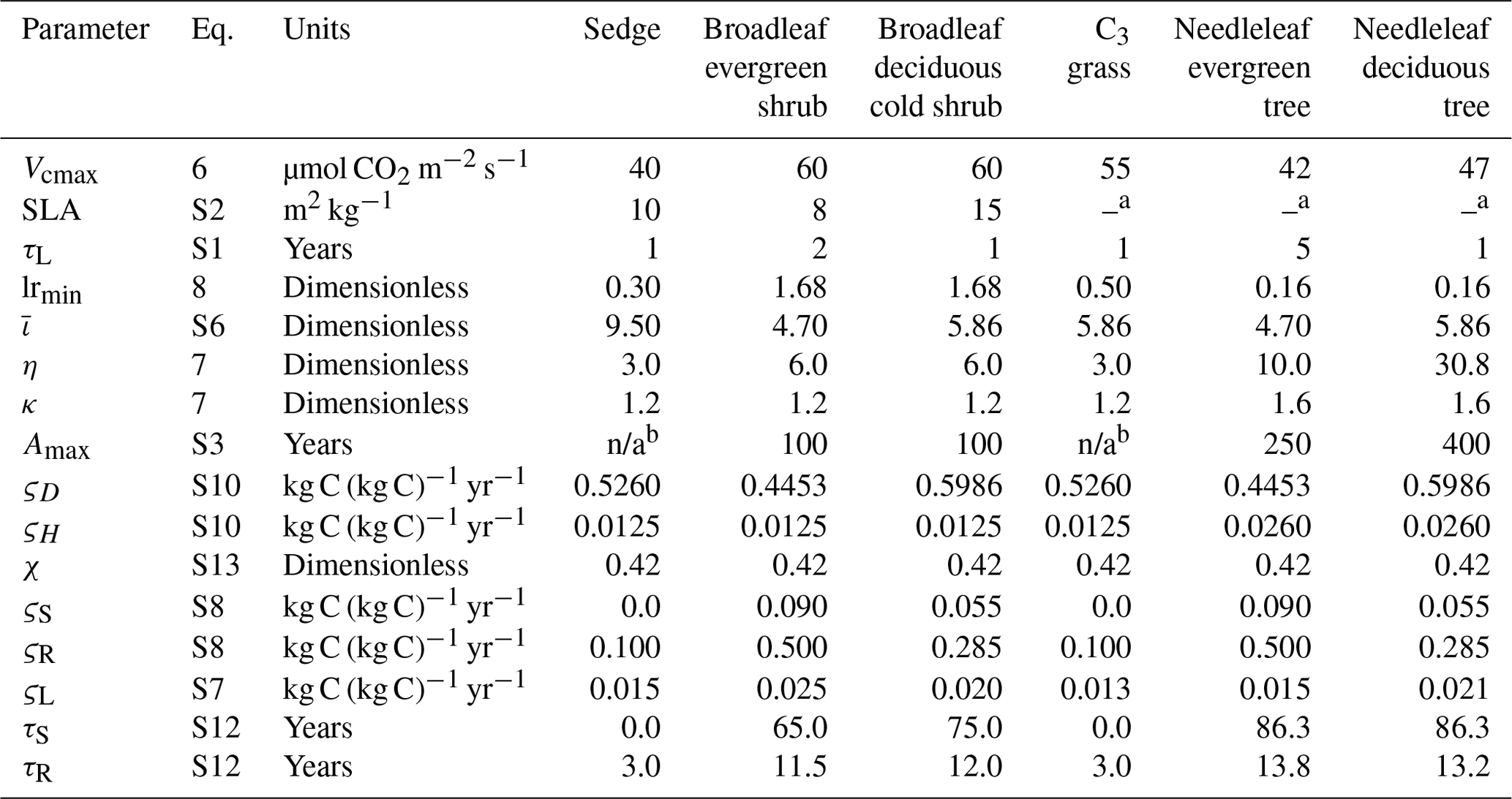
^a Determined by the model from the leaf life span. ^b In CLASSIC, A_max is not defined for grasses and sedges, as the age-related mortality is not applied to these PFTs. n/a – not applicable.

Download Print Version | Download XLSX

2.2 Model evaluation dataset

2.2.1 Study site

The study site at Daring Lake (AmeriFlux designation CA-DL1, hereafter referred to as DL1; 64^∘52.131^′ N, 111^∘34.498^′ W) is located in Canada's Northwest Territories, approximately 300 km northeast of Yellowknife, at an elevation of 425 m. The climate is characterized by short summers and long, cold winters with a mean annual air temperature of −8.9 ^∘C (Lafleur and Humphreys, 2018) and 200 to 300 mm of precipitation on average (ECG, 2012). In better-drained areas, the surface soil organic layer is typically shallow, ranging from 1 to 10 cm in depth, deepening to 20 cm or more in wetter areas, with all areas underlain by coarse textured mineral soil (sand to loamy sand) (Humphreys and Lafleur, 2011). The average thaw depth in late summer is 86 ± 3 cm (± SE) (Lafleur and Humphreys, 2018) measured over the period 2010–2015 using a metal probe inserted into the soil at 40 points (10 points every 5 m in the four cardinal directions around the measurement tower). DL1 is approximately 70 km north of the treeline in Canada's Southern Arctic ecozone (ECG, 2012). The dominant vegetation at DL1 includes evergreen shrubs (Rhododendron tomentosum, Empetrum nigrum, Loiseleuria procumbens) and deciduous shrubs (Betula glandulosa, Vaccinium uliginosum) (Lafleur and Humphreys, 2018). Small variations in microtopography result in wet areas covering about 10 % of the area within 200 m of the measurement tower, which support tussock-forming sedges and Sphagnum species. Growing season vascular plant cover at DL1 was 63.6 ± 5.4 % determined using point frame measurements in July 2019 at 10 quadrats with 25 points each. During the study period, the mean LAI during July measured using a plant canopy analyzer (model LAI-2200, LI-COR Inc., Lincoln, NE, USA, (LI-COR)) at 10 plots was 0.52 ± 0.05 (± SE) m² m⁻², mean height of shrubs was 18.2 ± 1.3 cm (Lafleur and Humphreys, 2018), and ground cover included mosses (percent ground cover: 16.5 ± 4.9 %) and lichens (78.9 ± 5.0 %) (Lafleur and Humphreys, 2018).

2.2.2 Measurements and data processing

Eddy covariance flux measurements

Eddy covariance measurements of turbulent CO₂ flux and energy fluxes and latent (LE) and sensible (H) heat flux have been made at DL1 during the growing season since 2004. The measurements and data processing are described in detail by Lafleur and Humphreys (2018). Briefly, the EC system consists of a CO₂–H₂O infrared gas analyzer (IRGA) and a three-dimensional sonic anemometer (model R3-50, Gill Instruments, Lymington, UK) operating at 10 Hz. The EC instrumentation is mounted to a mast 4.1 m above the surface, where 90 % of the total flux originates within 178 ± 21 m (± 1 standard deviation) from the flux tower determined using the flux footprint parameterization of Kljun et al. (2004). The tundra was well represented by the soil and vegetation characteristics described above for at least 400 m in all directions of the flux tower, and thus there was adequate fetch to represent this tundra type. An open-path IRGA (model LI-7500, LI-COR) was operated between 2004 and 2015, while an enclosed-path sensor (LI-7200, LI-COR) has been operated since 2014. The two IRGAs were run concurrently for 2014 and 2015 to develop a site-specific correction for the self-heating issue with the LI-7500 (Burba et al., 2008) described by Lafleur and Humphreys (2018). This correction was applied to all of the LI-7500 data. Half-hourly fluxes are calculated using EddyPro™ (v. 6.2.0) (LI-COR) with block averaging, a double coordinate rotation, and no angle of attack correction. When the open-path IRGA operated, density fluctuations were addressed using the Webb et al. (1980) approach; when the enclosed-path IRGA operated, fluxes were computed directly from ${CO}_{2} / H_{2} O$ mixing ratios. The covariance of the vertical wind speed and IRGA signals was used to compute time lags. Analytic correction of high- (Moncrieff et al., 2004) and low-pass (Moncrieff et al., 1997) filtering effects was applied. Half-hourly fluxes were removed from the time series due to sensor errors, due to power loss, or when associated variables (e.g., vertical velocity, CO₂–H₂O concentrations) were outside acceptable ranges. A 0.1 m s⁻¹ friction velocity threshold was applied to CO₂ fluxes at night and during snow-covered periods (Lafleur and Humphreys, 2008). Half-hourly net ecosystem productivity (NEP) was calculated as the sum of the CO₂ flux and the rate of change in CO₂ storage below the 4 m measurement height. The daily sum of turbulent energy fluxes did not equal available energy most days (e.g., mean daily $\frac{H + LE}{R_{n} - G}$ varied from 90 %–95 % mid-summer to 67 % on average during the snow-melt period (Fig. S5 in the Supplement); note that changes in energy storage between the EC instrumentation and the ground surface were not included in the evaluation of energy balance closure). LE and H were not adjusted for energy balance closure.

Half-hourly NEP was partitioned into GPP and ecosystem respiration (R_e) using methods similar to those described by Reichstein et al. (2005). An exponential temperature response function (Lloyd and Taylor, 1994) was parameterized using nighttime measurements of NEP (i.e., R_e) and T_a,

\begin{matrix} (9) & R_{e} = R_{ref} e^{E_{0} (\frac{1}{T_{ref} - T_{0}} - \frac{1}{T_{a} - T_{0}})}, \end{matrix}

where T_ref is set to 10 ^∘C and T₀ is −46.02 ^∘C. Equation (9) was first fit to the measurements within a moving window period of 15 d moved in increments of 5 d. The average of all temperature sensitivity (E₀) estimates which met the criteria (between 0 and 450 K) was calculated (144.7 K) and applied to Eq. (9) to estimate the temperature-independent respiration rate (R_ref) within consecutive 4 d periods. Finally, the constant E₀ and linearly interpolated R_ref values were used with Eq. (9) to calculate R_e for all daytime half hours and nighttime half hours without measurements, as a means to gap-fill nighttime NEP. GPP was calculated as the sum of NEP and R_e. Missing daytime half-hourly estimates of GPP were gap-filled by fitting a light response curve to all growing season GPP and photosynthetically active radiation (PAR) (Eq. 10) and adjusting the resulting GPP estimates by regressing these against previously estimated values within consecutive 4 d periods.

\begin{matrix} (10) & GPP = \frac{{GPP}_{max} α PAR}{α PAR + {GPP}_{max}}, \end{matrix}

where GPP_max (µmol m⁻² s⁻¹) is the maximum photosynthetic capacity at light saturation and α (mol CO₂ (mol PAR)⁻¹) the quantum efficiency.

Cold-season GPP was assumed to be negligible, and thus NEP was equal to R_e starting in the fall when the average T_a remained below −1 ^∘C for 3 consecutive days after 1 September of each year and until the snow had melted. Cold-season NEP and R_e were gap-filled using the average cold-season observations during the 4 d window period as Eq. (9) was often poorly fitted during these periods. CO₂ is removed from the atmosphere and taken up by the ecosystem when NEP and GPP values are positive. Positive R_e indicate an emission of CO₂ from the ecosystem to the atmosphere.

Latent heat flux was gap-filled using daytime and nighttime regressions between LE and available energy for all summer measurements. Estimates of LE were adjusted using a multiplier to match observed LE within 4 d consecutive periods. Sensible heat flux was gap-filled as the difference between available energy and gap-filled LE adjusted by a multiplier to account for changing energy budget imbalance. Daily total CO₂ and energy fluxes were calculated from gap-filled traces only when there were at least 8 half hours of measured fluxes which passed all QA/QC criteria.

Forced diffusion chamber measurements

In order to measure soil CO₂ efflux (assumed to represent R_e) during winter, three 10.1 cm diameter forced diffusion chambers (eosFD, Eosense Inc., Dartmouth, NS, Canada) were installed ∼ 50 m NW of the DL1 flux tower in a sandy, well-drained, and exposed area with little soil organic matter. Measurements were available from 18 August 2018 to 19 May 2019. Implausible eosFD fluxes (21 % of the time series) were excluded from analysis, including those indicating uptake of CO₂ exceeding 0.5 µmol CO₂ m⁻² s⁻¹ and those associated with atmospheric or internal concentrations below 400 ppm, which suggested problems with the analyzer's calibration, the diffusion membrane, or other factors related to gas transport through the frozen soil–snow–atmosphere system. Daily total CO₂ emissions were calculated from the average of the remaining measurements.

Meteorological measurements used to drive CLASSIC

CLASSIC runs were forced using 30 min meteorological observations at DL1 from 2004–2017. Measurements at DL1 included the four R_n components downwelling and upwelling shortwave and longwave radiation (CNR1, Kipp & Zonen B.V., Delft, the Netherlands), PA (PTB101B Barometer, Vaisala Oyj, Helsinki, Finland), T_a and relative humidity (RH) at 1.5 m height (HMP-35C, Vaisala), U and wind direction (propeller anemometer and wind vane at 1 m height; Wind Monitor, R.M. Young, Traverse City, MI, USA), rainfall (tipping bucket rain gauge, TE525M, Texas Electronics, Dallas, TX, USA), and snow depth (sonic distance sensor, SR50-L, CSI). Solid precipitation was estimated from increases in snow depth over a 30 min time step using a simple ratio of 1 mm water to 10 mm snow equivalent when T_a was below −2 ^∘C. Specific humidity was calculated as $q = \frac{e \cdot 0.622}{PA - e}$ , where $e = \frac{RH}{100} \cdot e_{s}$ with the vapour pressure e (Pa) and saturation vapour pressure e_s (Pa). Measurements of R_SW, R_LW, PA, T_a, RH, U, and rainfall were gap-filled using duplicate sensors at nearby Daring Lake weather stations and flux towers located within 2 km of the DL1 flux tower after adjusting for offsets. Any remaining gaps in PA, T_a, RH, and U were filled using the nearest Environment Canada observations at Whatì (63^∘8.018^′ N, 117^∘14.684^′ W; 271.3 m a.s.l.) after regressing available observations with DL1 to adjust for differences in elevation and climate. Remaining gaps in R_SW were filled with potential R_SW calculated using DL1's latitude and longitude following Stull (1988) and gaps in R_LW following Crawford and Duchon (1999) using gap-filled T_a and an estimate of cloud cover based on the ratio of gap-filled observed R_SW to potential R_SW. Precipitation was obtained from its two components, rainfall and snow depth increments converted to snow water equivalent using a factor of 10. Missing rainfall and snow depth increments were filled with Environment Canada Lupin station data (65^∘45.55^′ N, 111^∘15^′ W; 490.1 m a.s.l.) as these variables were not available from the Whatì station.

2.2.3 Further meteorological measurements used in this study

Additional weather observations at DL1 used in this study included up- and downwelling PAR (Quantum sensor, LI-190SA, LI-COR Inc.); soil temperatures (copper–constantan thermocouples) at 5, 25, and 60 cm depths; volumetric soil water content (VWC) (water content reflectometer, CS615, CSI) at 7 and 20 cm depths (beginning in late August 2015 for the 20 cm depth) in a drier area representative of the majority of the tower footprint; and G (soil heat flux plates at 7 cm depth, HFT3, CSI) adjusted to represent surface soil heat flux using the rate of change in energy stored in the layer of soil above the plates. PAR reflectivity was calculated as the ratio of upwelling to downwelling PAR.

Porosity, the liquid water content at wilting point, and other hydraulic and thermal soil properties are determined in CLASSIC using pedotransfer functions based upon the prescribed soil textures (Cosby et al., 1984; Clapp and Hornberger, 1978). For organic soils, peat type (fibric, hemic, or sapric)-dependent values are assigned to θ_p and wilting point following Letts et al. (2000). The modelled porosity and other soil properties did not necessarily correspond precisely to observed soil characteristics. For example, modelled θ_p for the surface organic layer and deeper mineral soil layers with 80 % sand content was 0.93 and 0.39 m³ m⁻³, respectively, while observed θ_p for the top 10 cm and deeper soil layers in the field was 0.77 and 0.46 m³ m⁻³, respectively. Although there may be differences in the absolute VWC (m³ m⁻³), the pore water held in the soil between field capacity and wilting point matric potentials are likely comparable. To facilitate this comparison, both observed and modelled VWC were scaled by their respective minimum and maximum values during 2004–2017 to produce a relative VWC value for each time step following

\begin{matrix} (11) & VWC (t) = (θ (t) - θ_{min}) / (θ_{p} - θ_{min}) . \end{matrix}

2.2.4 Bias-corrected reanalysis climate data

A merged, reanalysis-based atmospheric forcing dataset (GSWP3–W5E5–ERA5) was bias-corrected to the meteorological observations at DL1 and used to spin up and drive CLASSIC for the historical simulation over 1901–2004, when site observations were not available. The 1901–1978 portion of the GSWP3–W5E5–ERA5 dataset was extracted from the Inter-Sectoral Impact Model Intercomparison Project 0.5^∘ GSWP3–W5E5 atmospheric forcings (Kim, 2017; Lange, 2019, 2020 a, b) and bilinearly remapped to a 0.25^∘ grid. The 1979–2018 period is based on the 0.25^∘ ERA5 (ECMWF, 2019) time series that have been corrected so that long-term climatological means match those of the overlapping period of the GSWP3–W5E5 dataset.

Multivariate bias correction by an N-dimensional probability function transform (MBCn) (Cannon, 2018) was used to adjust daily R_SW, R_LW, minimum and maximum T_a, precipitation rate, PA, q, and U variables (1901–2018) from the GSWP3–W5E5–ERA5 data point nearest to DL1 to match the statistical characteristics – marginal distributions and multivariate dependence structure – of the in situ observations. GSWP3–W5E5–ERA5 data at the DL1 grid cell were adjusted using the 2004–2018 observational period for calibration, with MBCn applied over 15-year sliding windows from 1901–2018. In each window, the central year is replaced, the window is slid 1 year, the forcings are bias adjusted using MBCn, etc. until the end of the GSWP3–W5E5–ERA5 dataset is reached. To ensure an unbiased seasonal cycle, adjustments were applied over 30 d sliding intra-annual blocks of days. Outside of the 2004–2018 calibration period, changes in corrected quantiles were constrained to match those in the GSWP5–W5E5–ERA5 dataset; i.e., the adjustments are trend-preserving (Cannon et al., 2015).

After bias adjustment, daily variables were temporally disaggregated to the required 30 min time step following the same procedure as Melton and Arora (2016), where PA, q, and U are linearly interpolated and R_LW is uniformly distributed over the day. Dependent on DL1's latitude and the day of the year (DOY), R_SW and T_a are diurnally distributed (adapted from Cesaraccio et al., 2001). The daily amount of precipitation was used to determine the number of half hours during which precipitation occurred throughout the day (Arora, 1997) and was then randomly distributed over the wet half hours (Melton and Arora, 2016).

2.2.5 Simulations

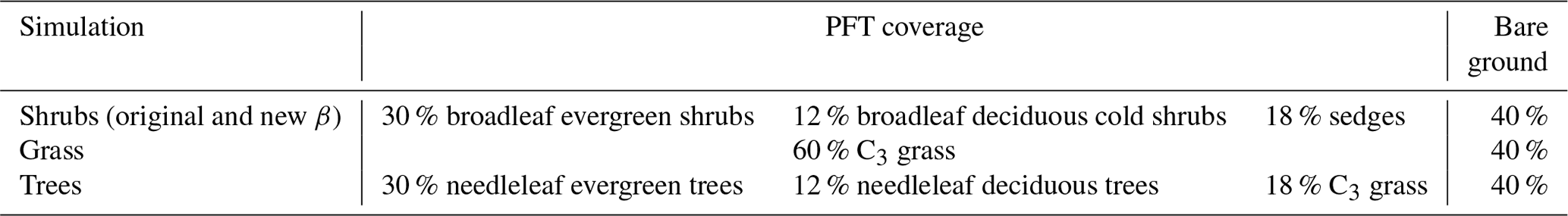
We performed three site-level simulations using different dominant PFT types (shrubs, grasses, and trees) and one simulation with the original β formulation (Eq. 4) with the shrub PFTs to illustrate the impacts of the model modifications on simulated energy and C fluxes and to compare with observations made at DL1. The fractional coverage of the PFTs used in the shrub, grass, and tree simulations for the DL1 site are shown in Table 3. For the shrub simulation, the broadleaf evergreen and broadleaf deciduous shrub and sedge cover reflect the vegetation observed at DL1. The grass simulation was set to C₃ grasses with an equivalent total plant cover (60 %). For the tree simulation, needleleaf evergreen trees and needleleaf deciduous trees were chosen for the PFTs as the dominant tree species around the treeline at the northern high latitudes are black and white spruce and larch (Sirois, 1992). For example, at DL1, which is only 70 km north of a diffuse treeline, sporadic clusters of stunted black spruce are present at the base of sheltered south-facing slopes. Bare ground fractional coverage was 40 % for all simulations, although at DL1 most of the ground not covered by vascular plants is covered by mosses and lichen.

Table 3Coverage of plant functional types (PFTs) used in the simulations.

Download Print Version | Download XLSX

The top 10 cm soil layer was set as a fibric organic layer (see Letts et al., 2000), with the deeper layers set as mineral soil consisting of 80 % sand, 4.4 % clay, and 3 % organic matter (apart from the second layer, which was assigned 8 % organic matter) to best reflect average soil characteristics observed at DL1. The bias-corrected GSWP3–ERA5 dataset for 1901–1925 was used repeatedly to drive the model until model C pools reached an equilibrium state, defined as a change in the annual C stocks of <0.1 %. The spin-up used the atmospheric CO₂ concentration from 1901 (Le Quéré et al., 2018). Starting from the equilibrium model spin-up state, a transient simulation was performed for the period 1901–2017 using time-varying CO₂ concentrations, the bias-corrected GSWP3–ERA5 meteorological forcing data for the years 1901–2003, and the meteorological observations from DL1 for the years 2004–2017 as forcing data for CLASSIC.

3 Results

3.1 Vegetation and soil carbon

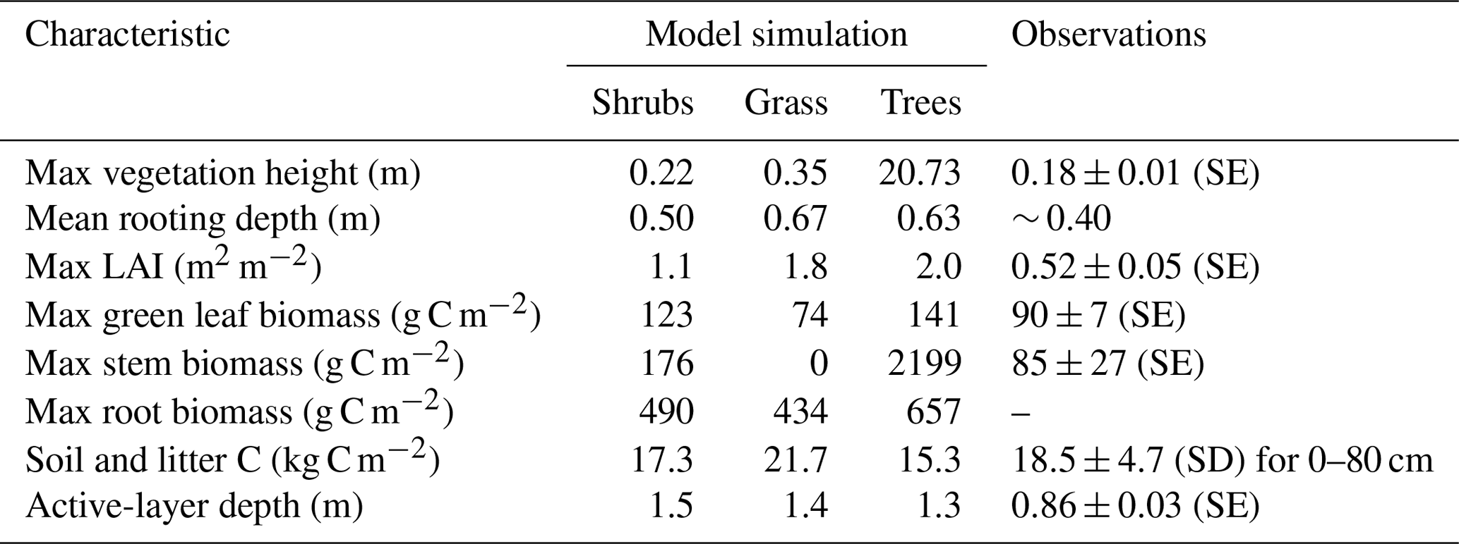
The three model simulations using shrub, grass, and tree PFTs produced vegetation with different characteristics (Table 4). Trees reached 20 m in height, while shrubs and grass remained below 0.35 m. The simulated shrub height of 0.22 m was very similar to observations at DL1 (Table 4).

As expected, simulated stem and root biomass were much larger for trees than shrubs, especially stem biomass. Green leaf biomass was similar for shrubs and trees but smaller for grass. Compared to observations, simulated shrub leaf and stem biomass were 1.4 and 2 times too high, respectively, but were an appropriate order of magnitude. The simulated ratio of stem to leaf biomass was 1.4 : 1, while the observed ratio was nearly 1 : 1, although there was variability among the three sample plots (ratios varied from 0.7 to 1.15). LAI was overestimated by all three simulations but was closest for the shrub simulation.

Each simulation produced detrital C pool (soil and litter C pools) estimates within the uncertainty bounds of the measured soil C at DL1, but again the shrub simulation was closest to the observed mean (Table 4).

Table 4Vegetation and soil characteristics observed at the Daring Lake tundra (DL1) research site and modelled for this site using three simulations of CLASSIC with different plant functional types and the new ground evaporation efficiency parameterization. Observations of vegetation height, LAI, and active-layer depth at DL1 are described in the Methods section. Mean rooting depth was approximated from visual observations in the field. Biomass was assessed by harvesting all standing living vascular vegetation from three 0.25 m² plots, sorting by species, and separating leaves and stems. Material was dried at 35 ^∘C to constant weight and converted to C assuming a 2 : 1 dry weight to C ratio. Soil C was assessed using loss on ignition and elemental C analysis of soil cores from eight random soil pits.

Download Print Version | Download XLSX

3.2 Soil temperature and moisture

Simulated mean daily soil temperatures (T_s) of model layers 1 (0–10 cm depth), 3 (20–30 cm depth), and 6 (50–60 cm depth) agreed well with field measurements between 2004 and 2017, with coefficients of determination (R²) between 90 % and 93 % and root-mean-square errors (RMSEs) between 2.2 and 2.5 ^∘C (Figs. 1 and S3 and Table S3). However, in deeper soil layers, simulated T_s was generally less seasonally variable than observations. As a result, simulated T_s was slightly warmer in winter and slightly cooler in summer (Fig. 1). This problem was exacerbated in the deeper layers with the original β formulation (Eq. 4; Fig. 1). Differences in daily T_s between the three simulations were small, but the shrub simulation showed slightly higher T_s year-round (Fig. S3), especially for layers 3 and 6, and agreed slightly better with measurements during summer (June through August). For example, the RMSE for layer 3 (20–30 cm) T_s was 1.6, 1.9, and 2.1 ^∘C and for layer 6 (50–60 cm) was 1.5, 1.7, and 1.9 ^∘C for the shrub, grass, and tree simulations, respectively. RMSEs were larger in winter for all simulations, with 2.7, 2.7, and 2.6 ^∘C for layer 3 and 2.6, 2.6, and 2.4 ^∘C for layer 6 for the shrub, grass, and tree simulations, respectively.

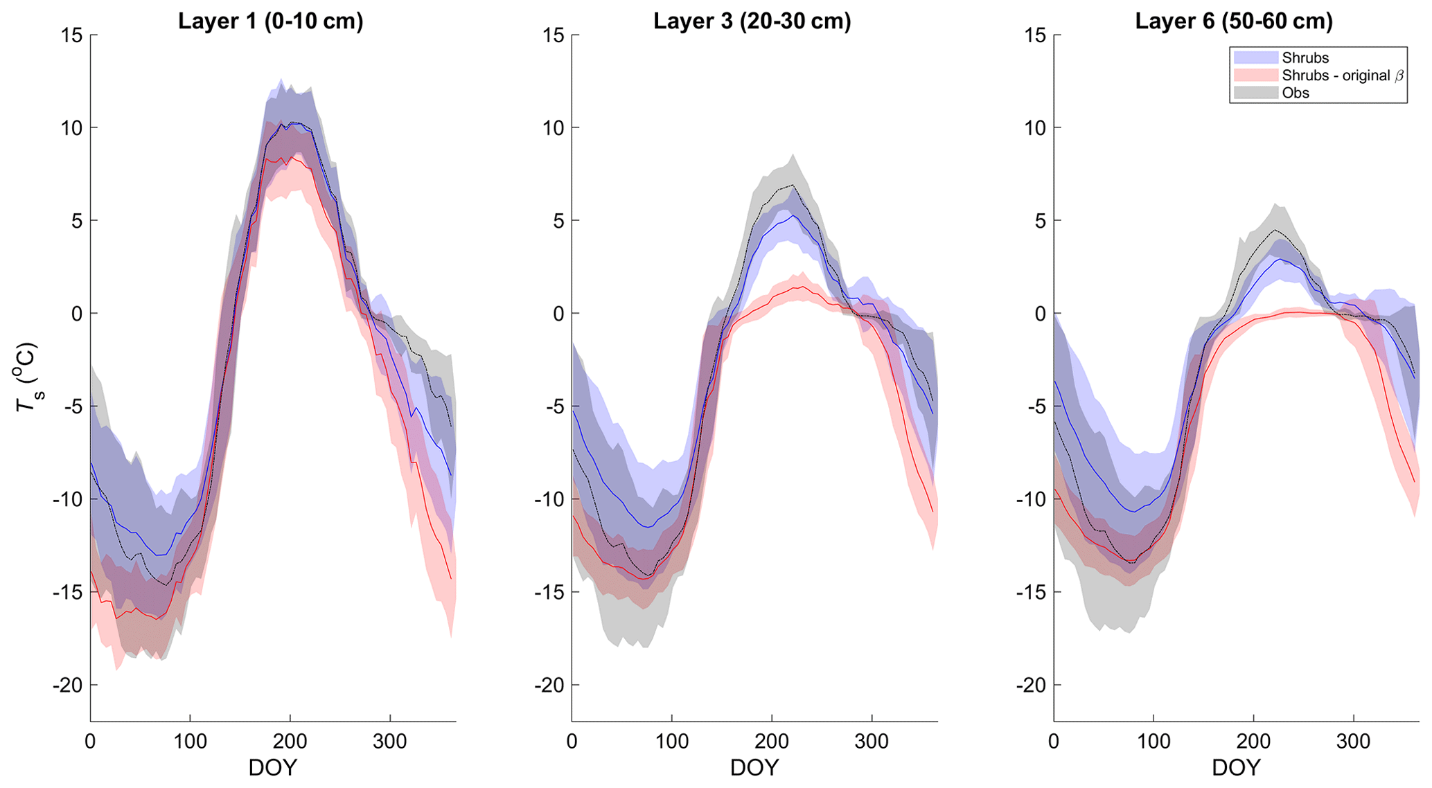
https://bg.copernicus.org/articles/18/3263/2021/bg-18-3263-2021-f01

Figure 1Mean 5 d average soil temperature for layer 1 (0–10 cm depth), 3 (20–30 cm depth), and 6 (50–60 cm depth) of the shrub simulations using the new (Merlin et al., 2011) and original β (Lee and Pielke, 1992) formulation compared to measurements at 5, 25, and 60 cm depth, respectively, averaged over 2004–2017. Shaded areas show the standard deviation of the daily mean for 2004–2017.

Download

All three simulations overestimated active-layer depth by 50 %–70 % compared to the average depth observed at DL1 (Table 4). Even though active-layer depths vary spatially at DL1, they have not been observed to exceed approximately 1.2 m. On average, simulated snow depth represented the observations well (Fig. 2). However, the model tended to be snow-free earlier than observations by 3 ± 4 d (mean ± SD) with a range of 11 d earlier to 5 d later.

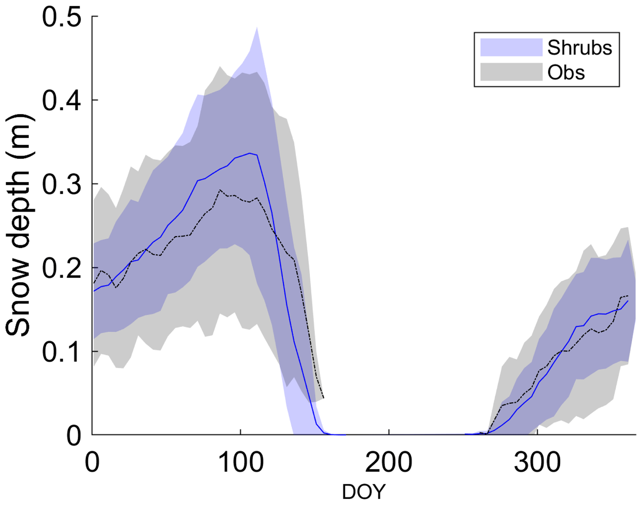
https://bg.copernicus.org/articles/18/3263/2021/bg-18-3263-2021-f02

Figure 2Mean observed and modelled 5 d average snow depth averaged over 2004–2017 for the shrub simulation. Shaded areas show the standard deviation of the daily mean for 2004–2017.

Download

Modelled mean daily relative VWC for the top soil layer (0–10 cm) averaged over 2004–2017 agreed reasonably well with relative VWC measured at 7 cm depth (Fig. 3a). Although interannual variability was high, VWC tended to be overestimated by the model around snowmelt and underestimated later in the growing season (early August to mid-October) regardless of PFT simulation. At the end of the growing season, the shrub simulation represented VWC the best; modelled relative VWC was lower than observed by 0.09, 0.17, and 0.18 m³ m⁻³ for the shrub, grass, and tree PFT simulations, respectively. Simulated end-of-growing-season relative VWC for the 10–20 cm layer was lower than observed by 0.11, 0.26, and 0.27 m³ m⁻³ for the shrub, grass, and tree PFT simulations, respectively. The original β formulation, which was known to overestimate ground evaporation (Sun and Verseghy, 2019), greatly underestimated relative VWC by on average 0.23 m³ m⁻³ for the top soil layer and 0.46 m³ m⁻³ for the 10–20 cm layer compared to observations throughout the growing season (Fig. 3).

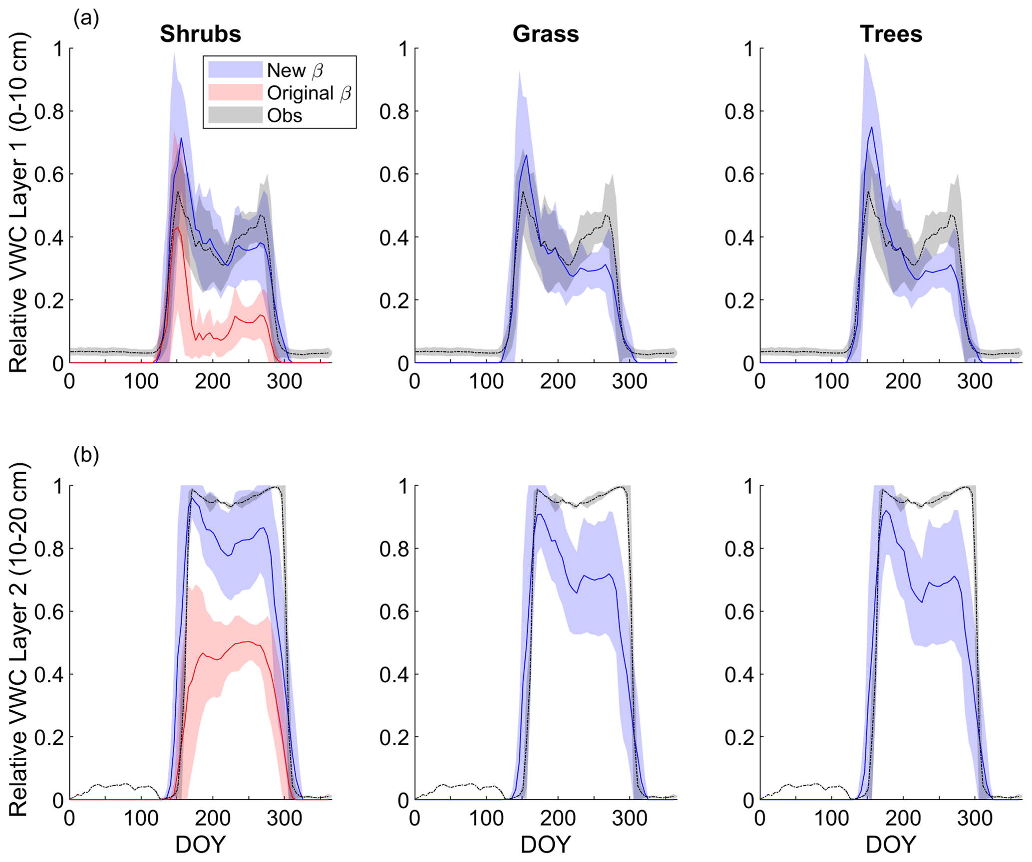
https://bg.copernicus.org/articles/18/3263/2021/bg-18-3263-2021-f03

Figure 3Mean 5 d average simulated relative volumetric water content (VWC, m³ m⁻³; see Eq. 11) (a) for the top model soil layer (0–10 cm depth) and observations at 7 cm depth and (b) for the second layer (10–20 cm depth) and observations measured at 20 cm depth averaged over 2004–2017 for the shrub, grass, and tree simulations. For the shrub simulation, results using the new (Merlin et al., 2011) and original β (Lee and Pielke, 1992) formulation are shown. Measurements at the 20 cm depth were only available starting late August 2015, while measurements at the 7 cm depth began in June 2004. Shaded areas show the standard deviation for 2004–2017 for the model results and observations at 7 cm depth and for 2015–2017 for observations at 20 cm depth.

Download

3.3 Turbulent energy fluxes (sensible and latent heat flux)

Differences in LE between the shrub, grass, and tree PFT simulations were relatively small on average (Fig. 4a). The adoption of the Merlin et al. (2011) β formulation reduced overestimation of LE by approximately 30 % during and just after snowmelt (mid-May to mid-June) (Fig. 4c). In summer, the new β formulation greatly reduced variability in LE and ensured there were no summer dates with unrealistically low LE (Fig. 4c). However, all three PFT simulations with the new β formulation still overestimated LE during and just after snowmelt and underestimated LE in summer (starting in late June). Average annual LE was 514, 397, 430, and 434 MJ m⁻² (or 16.3, 12.6, 13.6, and 13.8 W m⁻² d⁻¹ on average) for the observations, shrub simulations, grass simulations, and tree simulations, respectively. The observed annual value only includes data from DOY 95–310 as observations were not available for the whole year, but model results suggest that LE during the missing time period likely contributed very little (< 2 %) to the annual total.

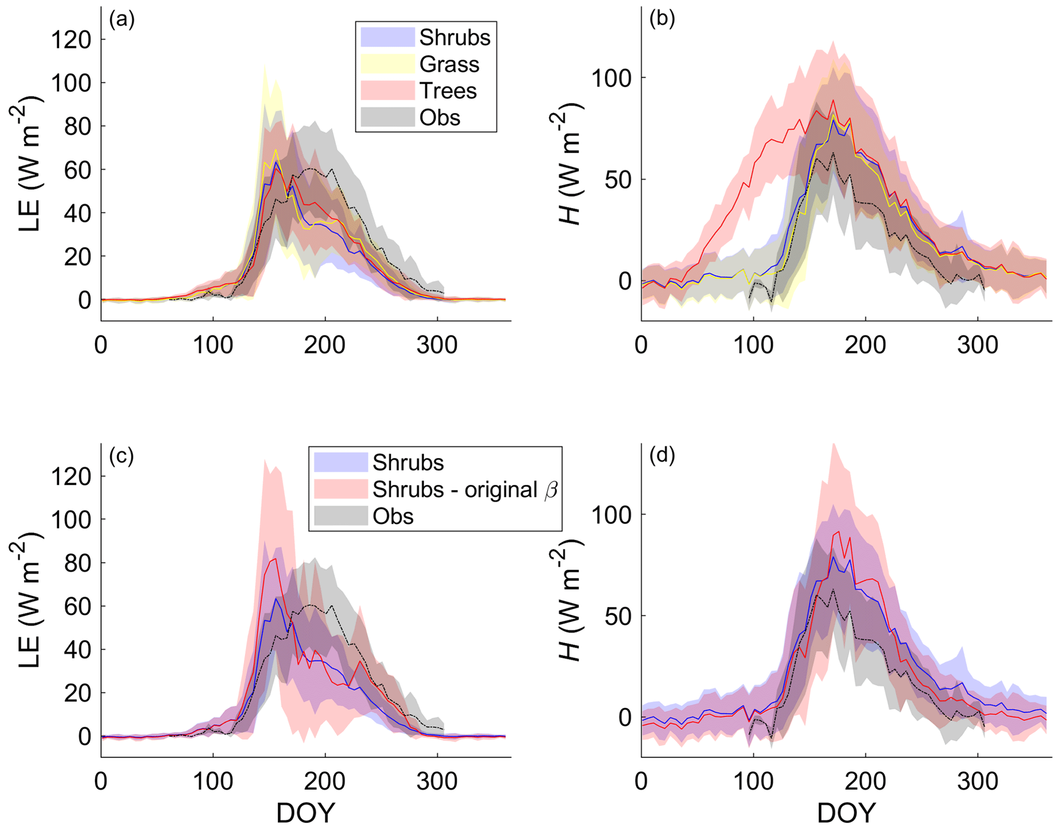
https://bg.copernicus.org/articles/18/3263/2021/bg-18-3263-2021-f04

Figure 4Mean 5 d average (a) latent (LE) and (b) sensible heat flux (H) over 2004–2017 for the shrub, grass, and tree simulations using the new β formulation (Merlin et al., 2011) and (c) LE and (d) H using the new and the original β formulation (Lee and Pielke, 1992) along with EC tower observations. Shaded areas show the standard deviation of the daily mean for 2004–2017.

Download

ET as simulated by the shrub PFT with the new β was dominated by ground evaporation (E) until mid-June, peaking shortly after snowmelt (Fig. 5). Ground E was slightly higher for the grass simulation and slightly lower for the tree simulation in spring compared to the shrub simulation (Fig. 5). Transpiration (T) was an important contributor to ET from mid-June to early September, peaking in early August. Maximum T was 40 %–45 % greater for the grass and tree PFT simulations compared to the shrub PFT simulation (Fig. 5), resulting in slightly greater ET (also shown as greater LE in Fig. 4a). For all three simulations, E of water intercepted by the canopy was a minor component of total ET.

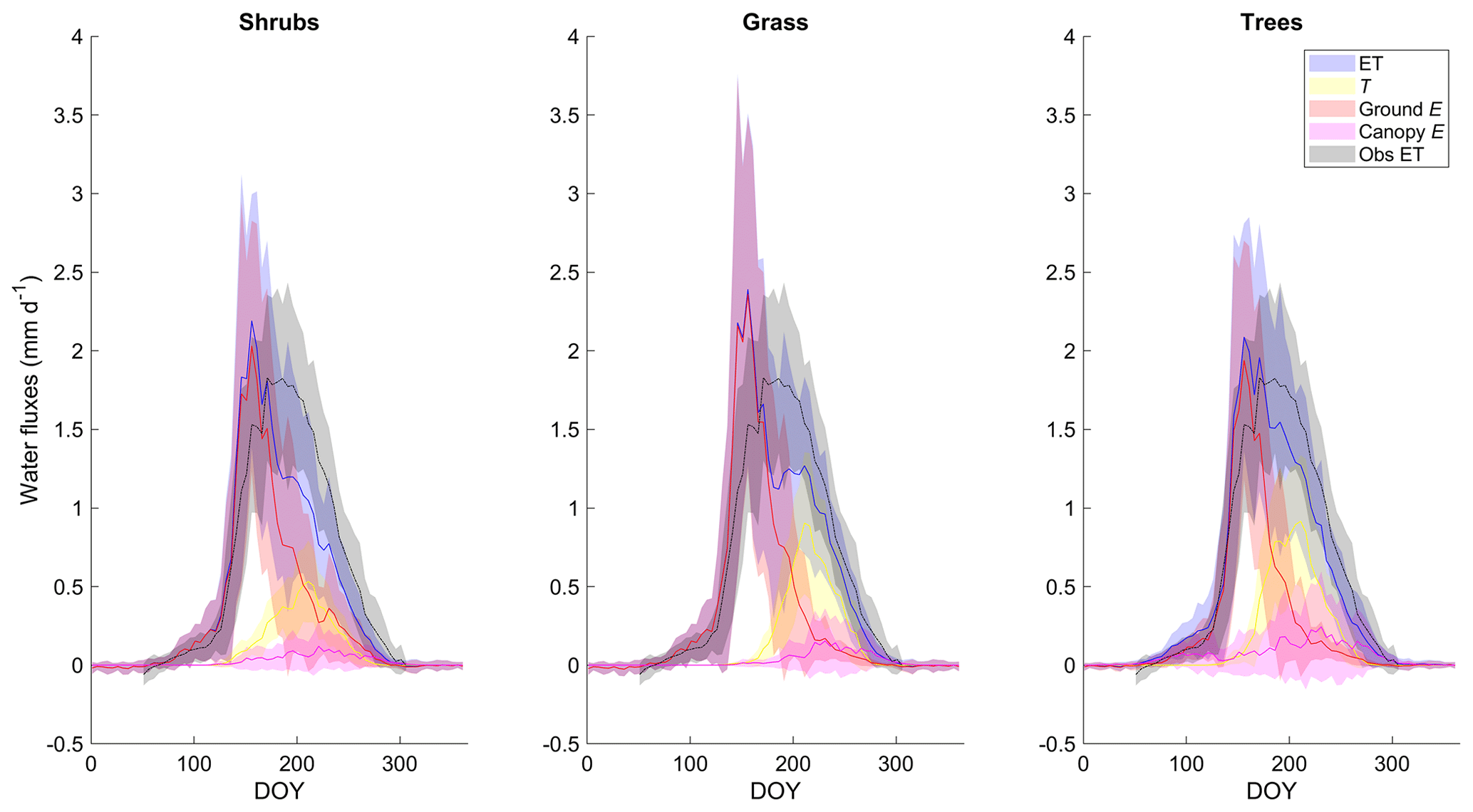
https://bg.copernicus.org/articles/18/3263/2021/bg-18-3263-2021-f05

Figure 5Mean 5 d average modelled evapotranspiration (ET) and its component fluxes (transpiration (T), ground and canopy evaporation (E)) along with observed ET averaged over 2004–2017 for the shrub, grass, and tree PFT simulations using the new β (Merlin et al., 2011) formulation. Shaded areas show the standard deviation of the daily mean for 2004–2017.

Download

For H, the shrub and grass simulations were similar, but the tree simulation greatly overestimated H especially from mid-April to the end of May (Fig. 4b). The average annual total H for the tree simulation (1046 MJ m⁻² or 33.2 W m⁻² d⁻¹) was about 1.5 times as large as for the shrub (659 MJ m⁻² or 20.9 W m⁻² d⁻¹) and grass simulations (605 MJ m⁻² or 19.2 W m⁻² d⁻¹) and more than 2.6 times the observed value (398 MJ m⁻² or 12.6 W m⁻² d⁻¹ for the period DOY 95–310). Only considering the time period where measurements were available, average H for the tree simulation was still 2.3 times the observed value. The original β formulation and shrub PFT simulation decreased H throughout the year except in summer, so it had relatively little impact on the annual H (592 MJ m⁻² or 18.8 W m⁻² d⁻¹) compared with the new β formulation (659 MJ m⁻² or 20.9 W m⁻² d⁻¹).

These large differences in spring H among PFT simulations could be linked to differences in simulated R_n (Fig. S6) and albedo (not shown). Albedo and R_n were similar for the shrub and grass simulations, with average albedo values of 0.91 and 0.92, respectively, during late winter, which was only slightly lower than the observed value of 0.97. The tree simulation, however, had a much larger R_n and lower albedo (0.55) than the shrub and grass simulations during winter, as the tall trees cannot be buried by snow.

3.4 Net ecosystem CO₂ exchange and its component fluxes

The shrub PFT simulation with the new β formulation best represented observed NEP and its component fluxes (Fig. 6 and Table 5). The new β formulation raised modelled VWC, reduced water stress, and supported GPP rates that closely resembled GPP derived from field observations at DL1. In contrast, the original β formulation resulted in GPP values that were only 26 % of observed values (Table 5 and Fig. S4). NEP simulated with the shrub PFT and new β formulation nevertheless was overestimated in spring as GPP started approximately 9 d earlier than observed, resulting in total growing season uptake that was 43 g C m² larger than observations (Table 5). In contrast, simulated total growing season R_e agreed well with observations (Table 5), although it was slightly higher than observed in spring and lower in summer (Fig. 6).

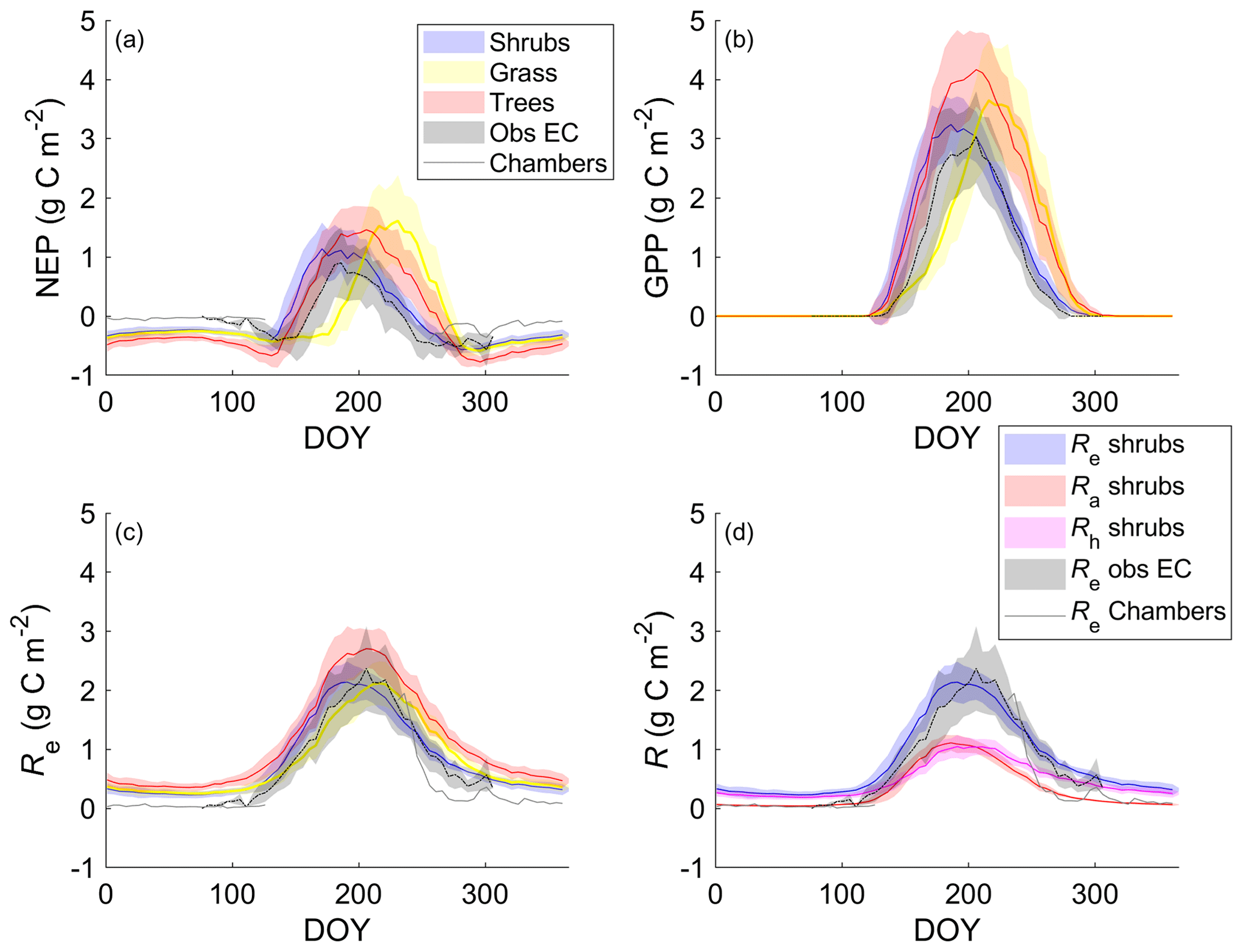
https://bg.copernicus.org/articles/18/3263/2021/bg-18-3263-2021-f06

Figure 6Mean 5 d average (a) net ecosystem productivity (NEP), (b) gross primary productivity (GPP), and (c) ecosystem respiration (R_e) for the shrub, grass, and tree simulations alongside EC tower-based observations. (d) Simulated R_e broken down into its component fluxes, autotrophic (R_a) and heterotrophic respiration (R_h), for the shrub simulation averaged over 2004–2017. Observed NEP (a) and R_e (c, d) include both EC measurements during the growing and shoulder seasons averaged over 2004–2017 and chamber measurements made between August 2018 and May 2019. Shaded areas show the standard deviation of the daily mean for 2004–2017.

Download

NEP simulated with the grass PFT lagged observations in the spring, peaking on average 49 d after the observations (Fig. 6a). Summer maximum GPP for the grass simulation was higher and, on average, reached a daily maximum 9 d later than observations. Simulated grass PFT GPP continued late into the fall, when observed GPP had declined to near zero. Total R_e was similar (Table 5) to R_e simulated with the shrub PFT, but again seasonal trends were offset by on average 10 d.

For the tree PFT simulation, simulated NEP and GPP were reasonably close to the measured values in the spring, although the start of NEP uptake was still about 10 d early (Fig. 6). Uptake was overestimated in mid-summer and into the fall compared to measurements, resulting in the largest growing season NEP (Table 5).

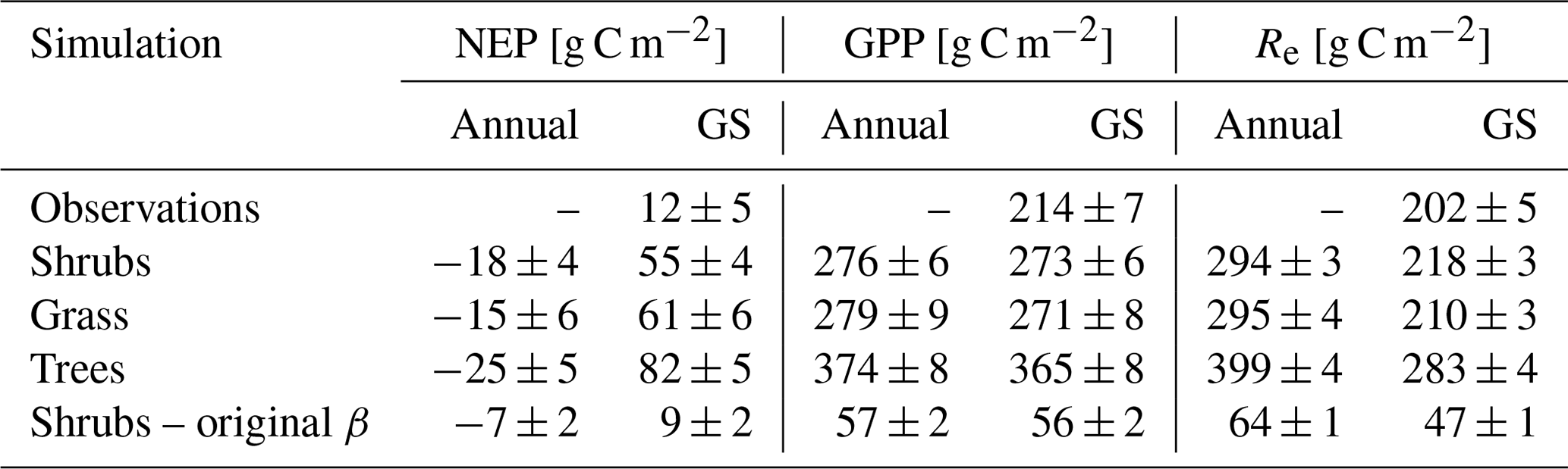
Table 5Mean ± SD annual and growing season (GS; 1 May–30 September) net ecosystem productivity (NEP), gross primary productivity (GPP), and ecosystem respiration (R_e) averaged over 2004–2017 for the shrub simulations using the new (Merlin et al., 2011) and original β (Lee and Pielke, 1992) formulation, for the grass and tree simulations, and for observations. Eddy covariance flux measurements were not available through the winter and are only reported for the growing season. Standard deviations (SDs) for the observed and simulated fluxes are calculated by error propagation of the SD of daily values.

Download Print Version | Download XLSX

Both chamber and EC measurements show a more rapid decrease in CO₂ emissions throughout September than shrub PFT simulations, as soil and air T dropped to or below 0 ^∘C (Fig. 6). However, EC flux observations in October and early November (DOY 275–309) were well represented by the NEP simulated using the shrub PFTs (Fig. 6). During the winter, from early November through March, when there were no EC measurements (DOY 310–365 and DOY 1–76), all three simulations had lower NEP and higher R_e than observed fluxes from the chambers (Fig. 6). However, the chamber-based observations have some significant uncertainties as fluxes were measured over one winter (fall 2018–spring 2019) only, which was outside the simulation period of 2004–2017. In addition, forced diffusion chambers have a much smaller footprint (41 cm²) with less diverse ground cover than the seasonal EC footprint of 10 ha or more.

During summer, the shrub simulation's R_a and R_h were roughly half of R_e (Fig. 6d). Fall and winter CO₂ emissions were primarily through R_h, although R_a remained above zero. Otherwise, R_a closely followed GPP trends. Similar patterns with slightly larger values were observed for the tree simulation, while the grass simulation's R_a was near zero for the winter months (Fig. S7).

All three model simulations suggest that DL1 was a net source of CO₂ over the 2004–2017 period (Fig. 7 and Table 5). Winter and shoulder season CO₂ emissions from October to April exceeded May through September CO₂ uptake by 26 %–32 % on average for the three simulations. Over the 14-year period, there was a net winter CO₂ loss of 211 g C m⁻² for grass, 254 g C m⁻² for shrub, and 344 g C m⁻² for tree simulations, which was equal to an average annual NEP of −15 to −25 g C m⁻² yr⁻¹ (Table 5). Bearing in mind the caveats discussed above regarding combining chamber and EC data streams, these simulated results were similar to an estimated NEP of −17 g C m⁻² yr⁻¹ obtained using these two sets of flux observations at DL1. The estimate of annual NEP was calculated from the sum of EC-based NEP (12 ± 5 g C m⁻²) for the 5-month growing season (Table 5), EC-based NEP ( $- 19 \pm 1$ g C m⁻²) for the 81 d that EC flux data were available during the shoulder seasons, and chamber-based NEP (−10 g C m⁻²) for the 131 d that winter EC fluxes were not available (Fig. 6).

The simulations of NEP differed in response to interannual variability in meteorological forcing (Table S2). On average, the 2010–2017 growing season was 2.1 ^∘C warmer and over 2 times wetter than 2004–2009 (two-tailed t-test p<0.05) (Table S2). NEP simulated using the grass PFT was more sensitive to these different weather conditions and thus more variable than the other two simulations over the study period, including a few years (2006, 2011, 2012, 2013, 2016, and 2017) where DL1 was simulated to be a net CO₂ sink. Annual net CO₂ uptake was also simulated for a few years (2011, 2012, 2013, and 2017) using the tree PFTs, while the shrub simulation only showed annual net CO₂ uptake in 2012.

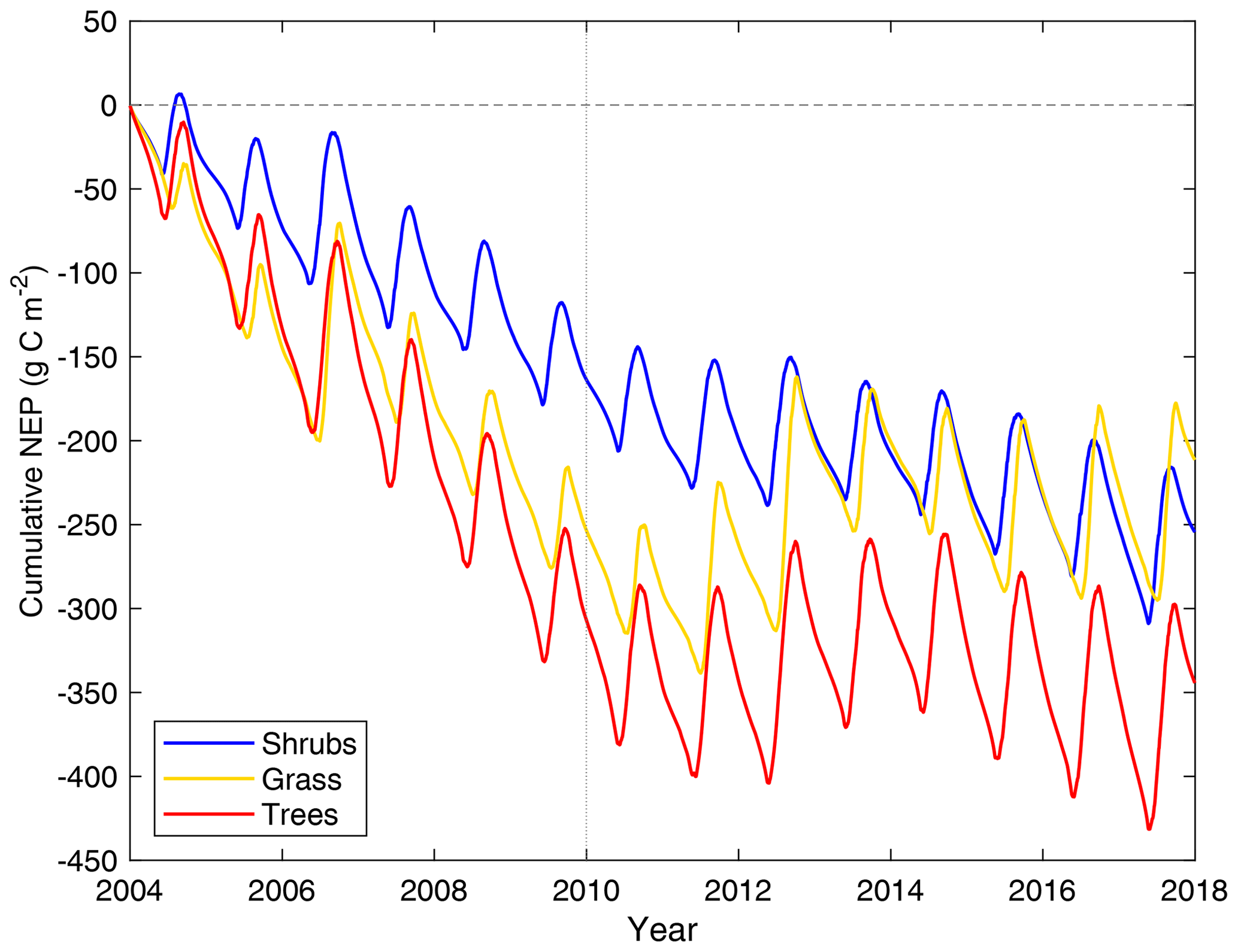
https://bg.copernicus.org/articles/18/3263/2021/bg-18-3263-2021-f07

Figure 7Cumulative daily modelled net ecosystem productivity (NEP) for 2004–2017 for the shrub, grass, and tree simulations. Negative values indicate the land surface was releasing CO₂ into the atmosphere. The vertical dotted line indicates the year marking a shift in weather, with colder and drier weather before 2010 and warmer and wetter weather thereafter.

Download

4 Discussion

Although we focus on high-latitude shrubs, shrubs are an important growth form in multiple regions and biomes; cover about 40 % of the land surface, including polar and alpine tundra, arid regions, and wetlands; and are often dominant within forest understories (Götmark et al., 2016). Shrubs, as a growth form, have a number of advantages compared to small trees. For example, in disturbed and low-productivity areas, shrubs have higher growth rates and, having multiple short or bendable stems, are more resilient to storm damage and weight of snow loading and can more readily recover from stem breakage and thus have higher survival rates under extreme conditions (Götmark et al., 2016).

This study highlights improved simulations of surface–atmosphere interactions at a Low Arctic upland tundra site in Canada with the introduction of shrub and sedge PFTs and an improved parameterization of ground evaporation within CLASSIC. We compare these results to other field and model studies that highlight key tundra ecosystem processes and the impacts of shrubs on evaporation, soil thermal regimes, and C cycling and storage.

4.1 Tundra–atmosphere water vapour exchange

This study addressed a high soil evaporation bias that has also been observed in other models' simulations of grasslands, wetlands, and forests, but especially in regions with sparse vegetation (Sun and Verseghy, 2019; Decker et al., 2017; Kauwe et al., 2017; Mu et al., 2021). The empirical formulation by Merlin et al. (2011) of the soil evaporation efficiency reduces simulated high rates of ground evaporation, particularly in spring, which avoided overdrying the 0–10 cm soil layer and greatly underestimating summer soil temperature, LE, and GPP, particularly in years with less summer rainfall. Although there were no field measurements to distinguish the soil moisture in the top few centimeters from the bottom few centimeters of this soil layer at DL1, it is clear from the high VWC at 20 cm depth that soils below the surface remain moist throughout the summer. As DL1 is located on a shallow slope below an esker, just west of several water tracks (channels of high moisture content in permafrost-dominated soils through which water is routed downslope; see Curasi et al. (2016) for a detailed description of these tundra features), which lead to a sedge wetland, it is expected that the DL1 site receives and sheds water through lateral flows, which CLASSIC does not simulate. Accordingly, Grant et al. (2015) found that lateral surface and subsurface flows were needed to model seasonal soil moisture variations at DL1 using the ecosystem model ecosys.

Even with the new β formulation, total ET and its main contributor, ground E, remained overestimated at the time of snowmelt, as demonstrated by simulated ET exceeding observed ET, likely due to a lack of infiltration into the porous surface soil. CLASSIC simulated ponded water during and up to ∼ 12 d after snowmelt resulting in saturated near-surface soil layers. In reality, water infiltrates into the soil faster with little ponding observed, as confirmed by repeat photography in the field. The ponding that did occur was generally within microtopographic depressions and for a shorter time period of about a week or less following snowmelt.

The empirical formulation by Merlin et al. (2011) of the soil evaporation efficiency can be adapted for different thicknesses of the top layer by using different soil-layer-thickness- and soil-texture-dependent values of the exponent in Eq. (5). Using the formulation of Merlin et al. (2011), CLASSIC's 10 cm thick top layer, however, was not able to represent a thin, dry surface layer reducing ground E. Attempts to reduce the top soil layer to 5 cm thickness or less created instabilities in the model. Excessive ground E was also observed in the Community Land Model (CLM), especially for sparse canopies or bare soil areas (Swenson and Lawrence, 2014). In order to address this issue, Swenson and Lawrence (2014) implemented a new soil resistance parameterization in the CLM version 4.5 that includes a dry surface layer whose thickness is determined from the moisture in the top soil layer and where evaporation is determined by water vapour diffusion through this layer. Using this parameterization in CLM resulted in less bias in ET, as soil E decreased due to higher resistances, even when soils were moist below the surface (Swenson and Lawrence, 2014). Another approach that could be employed in the future to prevent excessive ground E in CLASSIC is a representation of a litter layer increasing resistance to water vapour and heat exchange at the soil surface (e.g., Mu et al., 2021; Decker et al., 2017).

At DL1, the true proportion of total growing season ET partitioned to T is not known. However, a mini-lysimeter study was carried out during the last week of July 2019 to quantify ET partitioning. Four pairs of 25 cm diameter and ∼ 20 cm deep cores with vascular vegetation intact and vascular vegetation clipped at the ground surface were installed in pots set into the ground and reweighed. On average, T was 54 ± 29 % (SD) and 43 ± 25 % of ET after 1 and 2 d, respectively. Given the high variability among lysimeters, there was no evidence that T was significantly different than 50 % of total ET (two-tailed t-test p=0.71 and 0.46, respectively). CLASSIC also simulated ET to be 50 ± 22 % T for the last week of July 2004–2017 using the shrub PFT simulation with the new β formulation. This was a large increase over the shrub simulation with the original β formulation, where T was only 6 ± 5 % of ET, as shrub growth was greatly suppressed due to limiting soil moisture. The contribution of T to total ET for this period further increased with grass (64 ± 22 %) and tree (69 ± 22 %) PFT simulations. Intercomparisons of ESMs highlight that spatial variations in T : ET are largely driven by LAI, but many of these models underestimate the globally averaged ratio of T to ET compared to observations (Lian et al., 2018; Chang et al., 2018). Lian et al. (2018) suggested that model deficiencies in canopy light use, interception losses, and root water uptake processes contributed to the underestimation of T. Chang et al. (2018) found that inclusion of lateral flow and an improved representation of water vapour diffusion within the soil reduced E and increased T : ET, in agreement with the findings of Swenson and Lawrence (2014).

Because R_n was well represented but LE was underestimated in summer, the remaining energy had to be partitioned to other energy sinks. For the shrub PFT simulation with the new β formulation, there was an overestimate of thaw depth and growing season H. Nevertheless, soil temperatures in this permafrost-affected soil were reasonably well represented despite some dampened response at depth resulting in soils that are slightly warmer than observed in winter and colder in summer. Melton et al. (2019) showed that using a large number of soil layers (20) and greater depth of ground layers (61.4 m) than the three soil layers in previous model versions improved the simulation of circumpolar ground temperatures and active-layer depths in permafrost regions.

Due to trees remaining unburied by snow through the winter, the tree simulation did not represent R_n or H well during late winter. This shows the importance of accurately representing burial of vegetation by snow and/or representing vegetation dynamics in the model, such as shrub expansion and northward migration of the treeline, in order to predict current and future energy feedbacks to the climate system (e.g., Chapin et al., 2005). Recent studies have also noted the potential contribution of atmospheric moisture (through increased ET) feedbacks to regional warming of circumpolar regions through shifts in vegetation (Pearson et al., 2013; Bonfils et al., 2012; Lawrence and Swenson, 2011). Total annual T and ET over 2004–2017 were greater in our tree PFT simulation (56 ± 3 mm (± SD) and 162 ± 7 mm, respectively) over shrubs (34 ± 2 and 151 ± 8 mm, respectively). However, shrub T and ET were not greater than grass PFT T and ET (47 ± 3 and 164 ± 9 mm, respectively). Lafleur and Humphreys (2018) found there was little difference in growing season ET between DL1 and two neighbouring tundra sites with greater cover and height of shrubs. ET may not have differed among these and other tundra sites (McFadden et al., 1998, 2003), potentially due to compensation between ground E and T. In this study, ground E decreased slightly in the tree PFT simulation compared to the shrub PFT simulation, as T increased. However, further improvements to the model representation of the processes governing ET and additional evaluation with field data will improve our ability to characterize and quantify this potential climate feedback.

4.2 Shrub tundra CO₂ fluxes

Terrestrial ecosystem model estimates of annual CO₂ fluxes are especially useful in regions where year-round measurements are rare and difficult to obtain as they present a means to quantify the annual C budget of a region. The recent compilation by Natali et al. (2019) of CO₂ fluxes from over 100 high-latitude sites from the Arctic and boreal northern permafrost region during the winter season (October–April) confirmed that tundra ecosystems emit substantial amounts of CO₂ through the winter months. Of the three methods used in this study (EC, chamber, and model simulations), the rate of CO₂ emissions throughout the winter and shoulder seasons at DL1 was least with the chamber method and greatest in the model simulations. As noted earlier, differing scales of observation from <1 to 100 s of square meters for chambers and EC techniques, among other methodological differences, present issues when trying to compare results between the two methods and creating a continuous record of observations, particularly in ecosystems where fluxes are small and susceptible to methodological bias (Campioli et al., 2016). When compared for overlapping time periods (September 2018, not shown), chamber measurements of CO₂ fluxes were lower than the EC-derived R_e. Some of this difference may be due to the method used to partition NEP into R_e and GPP. Later in the season, as GPP declined to near zero with cold and snow-covered conditions and EC NEP was equal to −R_e, chamber R_e remained less than EC R_e. This difference was likely due to limited vegetation growth and survival within the chambers which remained in place and closed through the summer and winter. The three chambers were also located in well-drained sandy soils with minimal surface organic matter and thus did not represent the full tower footprint heterogeneity. For example, Campeau et al. (2014) reported a range in 0–50 cm soil organic C between 10 and 29 kg C m⁻² for the different vegetation communities characteristic of the DL1 flux tower footprint. Assuming R_e is influenced strongly by vegetation productivity, soil substrate, and soil temperature, among other drivers (Virkkala et al., 2018), it is reasonable to expect spatial variation in R_e.

CLASSIC NEP and R_e agreed well with EC observations through the fall and early winter, which was expected given that soil temperatures and detrital C stocks (soil and litter C) were well represented by the model. However, simulated R_e was on average 0.25 g C m⁻² d⁻¹ larger than EC-estimated R_e during late winter and early spring, which was likely a result of warmer modelled winter soil temperatures. This overestimation of winter R_e and its component fluxes, R_a and R_h, was higher for the tree than the shrub and grass PFT simulations. Both R_a and R_h contributed through the winter as a result of maintenance respiration of greater stem and root biomass and higher base soil respiration rates despite slightly cooler soil temperatures (Fig. S3). In tundra environments, vegetation traps drifting snow such that areas with taller and more abundant vegetation tend to have deeper snow and warmer winter soils (Sturm et al., 2005). CLASSIC does not include snow redistribution processes, which may have limited the differences in simulated winter soil temperatures among PFTs and would limit differences in related C cycle processes.

The ratio of winter CO₂ emissions to growing season uptake was tightly constrained between 1.26–1.32 for our simulations at DL1, which was lower than the estimate by Natali et al. (2019) of ∼ 1.61 for the northern Arctic and boreal permafrost region (growing season was defined here as May–September in accordance with Natali et al., 2019). This may be due to regional differences, overestimation of growing season uptake in our simulations, and uncertainties in the growing season uptake estimates from the process-based models they used. Our simulated winter emissions of 74–107 g C m⁻² yr⁻¹ at DL1, however, were within the range reported by Natali et al. (2019).

During and just after snowmelt, GPP was overestimated by CLASSIC for the shrub simulation and, to a lesser extent, the tree simulation. Commane et al. (2017) noted that this is a common problem in Earth system models, where most CMIP5 models simulated net CO₂ uptake earlier in spring than observed, contributing to an overestimation of annual net CO₂ uptake. In CLASSIC, this overestimation was likely due to a combination of simulated snowmelt occurring too early in the model and shrub productivity increasing too quickly after snowmelt completed. One possible reason for GPP overestimation in spring is that CLASSIC does not account for effects of pigments such as anthocyanin, which are produced by evergreen shrubs during fall and spring and peak shortly after snowmelt. Anthocyanin pigments cause reddening of the leaves and prevent photodamage to photosynthetic tissues when radiation levels are high, but T_a and T_s can be low (Oberbauer and Starr, 2002; Wyka and Oleksyn, 2014). Pigment concentrations have been measured to be elevated in shrubs in higher-light environments (e.g., little snow cover, upward facing leaves oriented towards the sky, or younger leaves with higher nitrogen content), resulting in lower photosynthetic capacity than in greener leaves (Oberbauer and Starr, 2002). CLASSIC does not simulate leaf reddening of evergreen shrubs in the spring, which could contribute to a high GPP bias in the model. Overestimation of GPP in the spring could also be related to the representation of phenology such as timing of leaf onset, especially for deciduous shrubs. The inclusion of a chilling requirement, in addition to growing degree days, has been shown to improve the timing of the initiation of C uptake and thus improve CO₂ flux simulations in other models, e.g., for northern Alaskan deciduous vegetation, especially during warm springs (Jeong et al., 2012; Shi et al., 2020). The limited availability of budburst measurements in tundra ecosystems and significant changes expected due to climate warming make improving modelled tundra phenology challenging (Diepstraten et al., 2018). Finally, the addition of the nitrogen cycle in CLASSIC may help reduce a high GPP bias as Low Arctic tundra plant growth is typically limited by nitrogen and phosphorus (e.g., Wieder et al., 2015; Wild et al., 2018).

Regardless of PFT simulation, CLASSIC simulated DL1 as a net source of CO₂ over the 14-year period. Although there was year-to-year variability in the magnitude of loss, including some years with net CO₂ uptake for the three simulations, average annual net CO₂ losses were not too different at 15 (grass PFT), 18 (shrub PFT), and 25 g C m⁻² yr⁻¹ (tree PFT). These net CO₂ loss estimates were similar to the combined EC and chamber estimate of 17 g C m⁻² yr⁻¹ as the overestimation of growing season net CO₂ uptake in the model was compensated for by an overestimation of winter CO₂ loss. Grant et al. (2011) – using the ecosys model, which included downslope lateral water flow (Grant et al., 2015) – found DL1 to be an annual C sink with net uptake of 17–45 g C m⁻² yr⁻¹ from 2004–2007, as modelled CO₂ losses between 1 September and 14 May were lower (24–31 g C m⁻²) than net CO₂ uptake of 41–76 g C m⁻² from 15 May–31 August. However, in agreement with our CLASSIC results, other permafrost-affected Arctic tundra ecosystems have also been observed and modelled as net sources of CO₂. For example, DL1's dwarf shrub tundra had similar net CO₂ losses to a heath tundra ecosystem in Alaska which lost on average 20 g C m⁻² yr⁻¹ or 158 ± 53 g C m⁻² over an 8-year period where soils consistently warmed (EC observations; Euskirchen et al., 2017). In that same region, wet sedge tundra was observed to lose 668 ± 83 g C m⁻² (or 84 g C m⁻² yr⁻¹) over 8 years (EC observations; Euskirchen et al., 2017). Further south in Alaska, thaw depth was observed to deepen over 6 years in moist acidic tundra, which lost a similar amount of CO₂ on average, 87 ± 17 g C m⁻² (EC observations; Celis et al., 2017), while in contrast the sedge-dominated Zackenberg fen of northeast Greenland was reported to be a net CO₂ sink of 50 g C m⁻² yr⁻¹ over a 10-year period, although 1 year had an annual loss of 21 g C m⁻² yr⁻¹ (EC observations combined with process model; López-Blanco et al., 2020).

In our study, the grass PFT simulation of NEP was more sensitive to environmental conditions, primarily through variations in growing season net CO₂ uptake (Fig. 7), when simulated growing season GPP increased more than R_a and R_h. A key factor increasing the sensitivity of the grass PFT's GPP to environmental conditions may be the lack of stems, enabling grasses to accumulate leaf mass more quickly than other PFTs. In the study by Euskirchen et al. (2017) noted above, the wet sedge tundra's annual net CO₂ exchange was also more variable than tussock and heath tundra, but in that study there was both less uptake and more loss during the growing and winter seasons, respectively, as soils warmed over time. Simulated shrub PFT NEP was less variable than observations at DL1 suggest. In a previous study at DL1, considerable variability in NEP from mid-May to the end of August strongly correlated to summertime ecosystem-level photosynthetic capacity, which could reflect differences in the amount and/or productivity of photosynthetic tissues through variations in nutrient availability, overwinter tissue damage, etc. (Humphreys and Lafleur, 2011).

5 Conclusions

CLASSIC's newly implemented shrub and sedge PFTs improved representation of soil temperatures, soil moisture, CO₂, and energy fluxes for a dwarf shrub tundra ecosystem, which was modelled to be a net CO₂ source over the 14-year study period. However, the timing of the onset of net CO₂ uptake in the spring was too early and contributed to the overestimation of growing season GPP and NEP. This issue may be resolved by incorporating leaf pigment dynamics and testing CLASSIC's new nitrogen cycle module (Asaadi and Arora, 2021) at the site. Another remaining issue is the overestimation of ET, particularly during the snowmelt period. The modified evaporation efficiency parameterization in CLASSIC was critical to represent observed soil temperatures and reduce soil drying that otherwise resulted in water stress limitations later in the growing season. However, ground evaporation and total ET remained high, which might be resolved by implementation of a dry surface soil or litter layer in the future.

Simulations of energy and CO₂ fluxes using shrub, grass, and tree PFTs demonstrated the importance of representing tundra ecosystems with the appropriate PFTs in Earth system models. The results of this study highlighted several important processes influenced by PFTs. For example, burial of vegetation by snow had a substantial impact on early-spring radiative and turbulent energy fluxes, PFT phenology and growth strategies influenced the timing and magnitude of net CO₂ uptake rates, and differences in C stocks along with surface energy exchange influenced the magnitude of winter CO₂ emission rates.

Code and data availability

The CLASSIC code v1.0.1 including shrub and sedge plant functional types is archived on Zenodo (https://doi.org/10.5281/zenodo.4301108; Meyer et al., 2020 a), and the eddy covariance and meteorological measurements made at the Daring Lake dwarf-shrub tundra site (DL1) between 2004 and 2017, which were used to drive and validate CLASSIC, are available on Zenodo as well (https://doi.org/10.5281/zenodo.4301133, Meyer et al., 2020 b).

Supplement

The supplement related to this article is available online at: https://doi.org/10.5194/bg-18-3263-2021-supplement.

Author contributions

GM tested and improved the parameterization of the new CLASSIC PFTs, performed the model simulations, and wrote the manuscript. ERH and JRM planned this study, helped set up the modelling framework and initialization files, and contributed to the analysis and manuscript. ERH and PML made the measurements at DL1 and processed the observation data. AJC bias-corrected the GSWP3–W5E5–ERA5 reanalysis data for the DL1 site. All authors contributed to the final manuscript.

Competing interests

The authors declare that they have no conflict of interest.

Acknowledgements

This research was funded through the Natural Sciences and Engineering Research Council of Canada and Polar Knowledge Canada. We thank Steve Matthews, Karin Clark, and the Daring Lake Terrestrial Ecosystem Research Station staff for logistical support; Michael Treberg for field and technical assistance; and graduate and undergraduate students for field assistance. We thank the two anonymous reviewers for their helpful comments and Vivek Arora for providing comments on a pre-submission version of the manuscript.

Review statement

This paper was edited by Paul Stoy and reviewed by two anonymous referees.

References

Abbott, B. W., Jones, J. B., Schuur, E. A. G., Chapin III, F. S., Bowden, W. B., Bret-Harte, M. S., Epstein, H. E., Flannigan, M. D., Harms, T. K., Hollingsworth, T. N., Mack, M. C., McGuire, A. D., Natali, S. M., Rocha, A. V., Tank, S. E., Turetsky, M. R., Vonk, J. E., Wickland, K. P., Aiken, G. R., Alexander, H. D., Amon, R. M. W., Benscoter, B. W., Bergeron, Y., Bishop, K., Blarquez, O., Bond-Lamberty, B., Breen, A. L., Buffam, I., Cai, Y., Carcaillet, C., Carey, S. K., Chen, J. M., Chen, H. Y. H., Christensen, T. R., Cooper, L. W., Cornelissen, J. H. C., de Groot, W. J., DeLuca, T. H., Dorrepaal, E., Fetcher, N., Finlay, J. C., Forbes, B. C., French, N. H. F., Gauthier, S., Girardin, M. P., Goetz, S. J., Goldammer, J. G., Gough, L., Grogan, P., Guo, L., Higuera, P. E., Hinzman, L., Hu, F. S., Hugelius, G., Jafarov, E. E., Jandt, R., Johnstone, J. F., Karlsson, J., Kasischke, E. S., Kattner, G., Kelly, R., Keuper, F., Kling, G. W., Kortelainen, P., Kouki, J., Kuhry, P., Laudon, H., Laurion, I., Macdonald, R. W., Mann, P. J., Martikainen, P. J., McClelland, J. W., Mo- lau, U., Oberbauer, S. F., Olefeldt, D., Paré, D., Parisien, M. A., Payette, S., Peng, C., Pokrovsky, O. S., Rastetter, E. B., Raymond, P. A., Raynolds, M. K., Rein, G., Reynolds, J. F., Robards, M., Rogers, B. M., Schädel, C., Schaefer, K., Schmidt, I. K., Shvidenko, A., Sky, J., Spencer, R. G. M., Starr, G., Striegl, R. G., Teisserenc, R., Tranvik, L. J., Virtanen, T., Welker, J. M., and Zimov, S.: Biomass offsets little or none of permafrost carbon release from soils, streams, and wildfire: an expert assessment, Environ. Res. Lett., 11, 034014, https://doi.org/10.1088/1748-9326/11/3/034014, 2016. a, b

Alton, P. B.: Retrieval of seasonal Rubisco-limited photosynthetic capacity at global FLUXNET sites from hyperspectral satellite remote sensing: Impact on carbon modelling, Agr. Forest Meteorol., 232, 74–88, https://doi.org/10.1016/j.agrformet.2016.08.001, 2017. a

Arndt, K. A., Lipson, D. A., Hashemi, J., Oechel, W. C., and Zona, D.: Snow melt stimulates ecosystem respiration in Arctic ecosystems, Global Change Biol., 26, 5042–5051, https://doi.org/10.1111/gcb.15193, 2020. a

Arora, V. K.: Land surface modelling in general circulation models: a hydrological perspective, PhD Thesis, Department of Civil and Environmental Engineering, University of Melbourne, 1997. a

Arora, V. K.: Simulating energy and carbon fluxes over winter wheat using coupled land surface and terrestrial ecosystem models, Agr. Forest Meteorol., 118, 21–47, https://doi.org/10.1016/S0168-1923(03)00073-X, 2003. a

Arora, V. K., Melton, J. R., and Plummer, D.: An assessment of natural methane fluxes simulated by the CLASS-CTEM model, Biogeosciences, 15, 4683–4709, https://doi.org/10.5194/bg-15-4683-2018, 2018. a

Asaadi, A. and Arora, V. K.: Implementation of nitrogen cycle in the CLASSIC land model, Biogeosciences, 18, 669–706, https://doi.org/10.5194/bg-18-669-2021, 2021. a

Bauerle, W. L., Oren, R., Way, D. A., Qian, S. S., Stoy, P. C., Thornton, P. E., Bowden, J. D., Hoffman, F. M., and Reynolds, R. F.: Photoperiodic regulation of the seasonal pattern of photosynthetic capacity and the implications for carbon cycling, P. Natl. Acad. Sci. USA, 109, 8612–8617, https://doi.org/10.1073/pnas.1119131109, 2012. a

Belshe, E. F., Schuur, E. A. G., Bolker, B. M., and Hooper, D.: Tundra ecosystems observed to be CO₂ sources due to differential amplification of the carbon cycle, Ecol. Lett., 16, 1307–1315, https://doi.org/10.1111/ele.12164, 2013a. a, b, c

Belshe, E. F., Schuur, E. A. G., and Grosse, G.: Quantification of upland thermokarst features with high resolution remote sensing, Environ. Res. Lett., 8, 035016, https://doi.org/10.1088/1748-9326/8/3/035016, 2013b. a

Bonfils, C. J. W., Phillips, T. J., Lawrence, D. M., Cameron-Smith, P., Riley, W. J., and Subin, Z. M.: On the influence of shrub height and expansion on northern high latitude climate, Environ. Res. Lett., 7, 015503, https://doi.org/10.1088/1748-9326/7/1/015503, 2012. a

Burba, G. G., McDermitt, D. K., Grelle, A., Anderson, D. J., and Xu, L.: Addressing the influence of instrument surface heat exchange on the measurements of CO₂ flux from open-path gas analyzers, Global Change Biol., 14, 1854–1876, https://doi.org/10.1111/j.1365-2486.2008.01606.x, 2008. a

Campioli, M., Malhi, Y., Vicca, S., Luyssaert, S., Papale, D., Peñuelas, J., Reichstein, M., Migliavacca, M., Arain, M. A., and Janssens, I. A.: Evaluating the convergence between eddy-covariance and biometric methods for assessing carbon budgets of forests, Nat. Commun., 7, 13717, https://doi.org/10.1038/ncomms13717, 2016. a

Cannon, A. J.: Multivariate quantile mapping bias correction: an N-dimensional probability density function transform for climate model simulations of multiple variables, Clim. Dynam., 50, 31–49, https://doi.org/10.1007/s00382-017-3580-6, 2018. a

Cannon, A. J., Sobie, S. R., and Murdock, T. Q.: Bias Correction of GCM Precipitation by Quantile Mapping: How Well Do Methods Preserve Changes in Quantiles and Extremes?, J. Climate, 28, 6938–6959, https://doi.org/10.1175/jcli-d-14-00754.1, 2015. a

Celis, G., Mauritz, M., Bracho, R., Salmon, V. G., Webb, E. E., Hutchings, J., Natali, S. M., Schädel, C., Crummer, K. G., and Schuur, E. A. G.: Tundra is a consistent source of CO₂ at a site with progressive permafrost thaw during 6 years of chamber and eddy covariance measurements, J. Geophys. Res.-Biogeo., 122, 1471–1485, https://doi.org/10.1002/2016jg003671, 2017. a

Cesaraccio, C., Spano, D., Duce, P., and Snyder, R. L.: An improved model for determining degree-day values from daily temperature data, Int. J. Biometeorol., 45, 161–169, https://doi.org/10.1007/s004840100104, 2001. a

Chang, L., Dwivedi, R., Knowles, J. F., Fang, Y., Niu, G., Pelletier, J. D., Rasmussen, C., Durcik, M., Barron-Gafford, G. A., and Meixner, T.: Why Do Large-Scale Land Surface Models Produce a Low Ratio of Transpiration to Evapotranspiration?, J. Geophys. Res.-Atmos., 123, 9109–9130, https://doi.org/10.1029/2018JD029159, 2018. a, b

Chapin, F. S. and Shaver, G. R.: Arctic, in: Physiological Ecology of North American Plant Communities, Springer, Dordrecht, The Netherlands, 16–40, https://doi.org/10.1007/978-94-009-4830-3_2, 1985. a, b

Chapin, F. S., Sturm, M., Serreze, M. C., McFadden, J. P., Key, J. R., Lloyd, A. H., McGuire, A. D., Rupp, T. S., Lynch, A. H., Schimel, J. P., Beringer, J., Chapman, W. L., Epstein, H. E., Euskirchen, E. S., Hinzman, L. D., Jia, G., Ping, C. L., Tape, K. D., Thompson, C. D. C., Walker, D. A., and Welker, J. M.: Role of Land-Surface Changes in Arctic Summer Warming, Science, 310, 657–660, https://doi.org/10.1126/science.1117368, 2005. a, b

Ciais, P., Tan, J., Wang, X., Roedenbeck, C., Chevallier, F., Piao, S.-L., Moriarty, R., Broquet, G., Quéré, C. L., Canadell, J. G., Peng, S., Poulter, B., Liu, Z., and Tans, P.: Five decades of northern land carbon uptake revealed by the interhemispheric CO₂ gradient, Nature, 568, 221–225, https://doi.org/10.1038/s41586-019-1078-6, 2019. a

Clapp, R. B. and Hornberger, G. M.: Empirical equations for some soil hydraulic properties, Water Resour. Res., 14, 601–604, https://doi.org/10.1029/wr014i004p00601, 1978. a

Commane, R., Lindaas, J., Benmergui, J., Luus, K. A., Chang, R. Y. W., Daube, B. C., Euskirchen, E. S., Henderson, J. M., Karion, A., Miller, J. B., Miller, S. M., Parazoo, N. C., Randerson, J. T., Sweeney, C., Tans, P. P., Thoning, K., Veraverbeke, S., Miller, C. E., and Wofsy, S. C.: Carbon dioxide sources from Alaska driven by increasing early winter respiration from Arctic tundra, P. Natl. Acad. Sci. USA, 114, 5361–5366, https://doi.org/10.1073/pnas.1618567114, 2017. a, b, c, d, e

Cosby, B. J., Hornberger, G. M., Clapp, R. B., and Ginn, T. R.: A Statistical Exploration of the Relationships of Soil Moisture Characteristics to the Physical Properties of Soils, Water Resour. Res., 20, 682–690, https://doi.org/10.1029/wr020i006p00682, 1984. a

Crawford, T. M. and Duchon, C. E.: An Improved Parameterization for Estimating Effective Atmospheric Emissivity for Use in Calculating Daytime Downwelling Longwave Radiation, J. Appl. Meteorol. Clim., 38, 474–480, https://doi.org/10.1175/1520-0450(1999)038<0474:AIPFEE>2.0.CO;2, 1999. a

Curasi, S. R., Loranty, M. M., and Natali, S. M.: Water track distribution and effects on carbon dioxide flux in an eastern Siberian upland tundra landscape, Environ. Res. Lett., 11, 045002, https://doi.org/10.1088/1748-9326/11/4/045002, 2016. a

Decker, M., Or, D., Pitman, A., and Ukkola, A.: New turbulent resistance parameterization for soil evaporation based on a pore-scale model: Impact on surface fluxes in CABLE, J. Adv. Model. Earth Sy., 9, 220–238, https://doi.org/10.1002/2016ms000832, 2017. a, b

Diepstraten, R. A. E., Jessen, T. D., Fauvelle, C. M. D., and Musiani, M. M.: Does climate change and plant phenology research neglect the Arctic tundra?, Ecosphere, 9, e02362, https://doi.org/10.1002/ecs2.2362, 2018. a

Ecosystem Classification Group (ECG): Ecological Regions of the Northwest Territories – Southern Arctic, Department of Environment and Natural Resources, Government of the Northwest Territories, Yellowknife, Northwest Territories, Canada, Tech. Rep., https://doi.org/10.13140/RG.2.1.3219.0165, 2012. a, b

European Centre for Medium-Range Weather Forecasts (ECMWF): ERA5 Reanalysis (0.25^∘ Latitude-Longitude Grid), Research Data Archive at the National Center for Atmospheric Research, Computational and Information Systems Laboratory, https://doi.org/10.5065/BH6N-5N20, 2019. a

Euskirchen, E. S., Bret-Harte, M. S., Shaver, G. R., Edgar, C. W., and Romanovsky, V. E.: Long-Term Release of Carbon Dioxide from Arctic Tundra Ecosystems in Alaska, Ecosystems, 20, 960–974, https://doi.org/10.1007/s10021-016-0085-9, 2017. a, b, c, d

Götmark, F., Götmark, E., and Jensen, A. M.: Why Be a Shrub? A Basic Model and Hypotheses for the Adaptive Values of a Common Growth Form, Front. Plant Sci., 7, 1095, https://doi.org/10.3389/fpls.2016.01095, 2016. a, b

Grant, R. F., Humphreys, E. R., Lafleur, P. M., and Dimitrov, D. D.: Ecological controls on net ecosystem productivity of a mesic arctic tundra under current and future climates, J. Geophys. Res., 116, G01031, https://doi.org/10.1029/2010JG001555, 2011. a

Grant, R. F., Humphreys, E. R., and Lafleur, P. M.: Ecosystem CO₂ and CH₄ exchange in a mixed tundra and a fen within a hydrologically diverse Arctic landscape: 1. Modeling versus measurements: CO₂ and CH₄ Exchange in the Arctic, J. Geophys. Res.-Biogeo., 120, 1366–1387, 2015. a, b

Grogan, P. and Chapin III, F. S.: Initial effects of experimental warming on above- and belowground components of net ecosystem CO₂ exchange in arctic tundra, Oecologia, 125, 512–520, https://doi.org/10.1007/s004420000490, 2000. a

Hayes, D. J., Kicklighter, D. W., McGuire, A. D., Chen, M., Zhuang, Q., Yuan, F., Melillo, J. M., and Wullschleger, S. D.: The impacts of recent permafrost thaw on land-atmosphere greenhouse gas exchange, Environ. Res. Lett., 9, 045005, https://doi.org/10.1088/1748-9326/9/4/045005, 2014. a, b

Hugelius, G., Strauss, J., Zubrzycki, S., Harden, J. W., Schuur, E. A. G., Ping, C.-L., Schirrmeister, L., Grosse, G., Michaelson, G. J., Koven, C. D., O'Donnell, J. A., Elberling, B., Mishra, U., Camill, P., Yu, Z., Palmtag, J., and Kuhry, P.: Estimated stocks of circumpolar permafrost carbon with quantified uncertainty ranges and identified data gaps, Biogeosciences, 11, 6573–6593, https://doi.org/10.5194/bg-11-6573-2014, 2014. a

Humphreys, E. R. and Lafleur, P. M.: Does earlier snowmelt lead to greater CO₂ sequestration in two low Arctic tundra ecosystems?, Geophys. Res. Lett., 38, L09703, https://doi.org/10.1029/2011GL047339, 2011. a, b

Huntzinger, D. N., Schaefer, K., Schwalm, C., Fisher, J. B., Hayes, D., Stofferahn, E., Carey, J., Michalak, A. M., Wei, Y., Jain, A. K., Kolus, H., Mao, J., Poulter, B., Shi, X., Tang, J., and Tian, H.: Evaluation of simulated soil carbon dynamics in Arctic-Boreal ecosystems, Environ. Res. Lett., 15, 025005, https://doi.org/10.1088/1748-9326/ab6784, 2020. a

Intergovernmental Panel on Climate Change (IPCC): Climate Change 2014: Impacts, Adaptation and Vulnerability, Part A: Global and Sectoral Aspects, in: Contribution of Working Group II to the Fifth Assessment Report of the Intergovernmental Panel on Climate Change, Tech. Rep., Cambridge University Press, Cambridge, United Kingdom and New York, NY, USA, 1132 pp., 2014. a

Jeong, S.-J., Medvigy, D., Shevliakova, E., and Malyshev, S.: Uncertainties in terrestrial carbon budgets related to spring phenology, J. Geophys. Res.-Biogeo., 117, G01030, https://doi.org/10.1029/2011jg001868, 2012. a

Jeong, S.-J., Bloom, A. A., Schimel, D., Sweeney, C., Parazoo, N. C., Medvigy, D., Schaepman-Strub, G., Zheng, C., Schwalm, C. R., Huntzinger, D. N., Michalak, A. M., and Miller, C. E.: Accelerating rates of Arctic carbon cycling revealed by long-term atmospheric CO₂ measurements, Science Advances, 4, eaao1167, https://doi.org/10.1126/sciadv.aao1167, 2018. a

Kauwe, M. G. D., Medlyn, B. E., Walker, A. P., Zaehle, S., Asao, S., Guenet, B., Harper, A. B., Hickler, T., Jain, A. K., Luo, Y., Lu, X., Luus, K., Parton, W. J., Shu, S., Wang, Y.-P., Werner, C., Xia, J., Pendall, E., Morgan, J. A., Ryan, E. M., Carrillo, Y., Dijkstra, F. A., Zelikova, T. J., and Norby, R. J.: Challenging terrestrial biosphere models with data from the long-term multifactor Prairie Heating and CO₂ Enrichment experiment, Global Change Biol., 23, 3623–3645, https://doi.org/10.1111/gcb.13643, 2017. a

Kim, H.: Global Soil Wetness Project Phase 3 Atmospheric Boundary Conditions (Experiment 1) [Data set], Data Integration and Analysis System (DIAS), https://doi.org/10.20783/DIAS.501, 2017. a

Kljun, N., Calanca, P., Rotach, M. W., and Schmid, H. P.: A Simple Parameterisation for Flux Footprint Predictions, Bound.-Lay. Meteorol., 112, 503–523, https://doi.org/10.1023/B:BOUN.0000030653.71031.96, 2004. a

Lafleur, P. M. and Humphreys, E. R.: Spring warming and carbon dioxide exchange over low Arctic tundra in central Canada, Global Change Biol., 14, 740–756, https://doi.org/10.1111/j.1365-2486.2007.01529.x, 2008. a

Lafleur, P. M. and Humphreys, E. R.: Tundra shrub effects on growing season energy and carbon dioxide exchange, Environ. Res. Lett., 13, 055001, https://doi.org/10.1088/1748-9326/aab863, 2018. a, b, c, d, e, f, g, h

Lange, S.: WFDE5 over land merged with ERA5 over the ocean (W5E5), V. 1.0, GFZ Data Services, https://doi.org/10.5880/pik.2019.023, 2019. a

Lange, S.: The Inter-Sectoral Impact Model Intercomparison Project Input data set: GSWP3-W5E5, available at: https://www.isimip.org/gettingstarted/input-data-bias-correction/details/80/, last access: 10 June 2020a. a

Lange, S.: ISIMIP3BASD (Version 2.3), Zenodo, https://doi.org/10.5281/zenodo.3648654, 2020b. a

Lantz, T. C., Marsh, P., and Kokelj, S. V.: Recent Shrub Proliferation in the Mackenzie Delta Uplands and Microclimatic Implications, Ecosystems, 16, 47–59, https://doi.org/10.1007/s10021-012-9595-2, 2012. a

Lawrence, D. M. and Swenson, S. C.: Permafrost response to increasing Arctic shrub abundance depends on the relative influence of shrubs on local soil cooling versus large-scale climate warming, Environ. Res. Lett., 6, 045504, https://doi.org/10.1088/1748-9326/6/4/045504, 2011. a

Le Quéré, C., Andrew, R. M., Friedlingstein, P., Sitch, S., Hauck, J., Pongratz, J., Pickers, P. A., Korsbakken, J. I., Peters, G. P., Canadell, J. G., Arneth, A., Arora, V. K., Barbero, L., Bastos, A., Bopp, L., Chevallier, F., Chini, L. P., Ciais, P., Doney, S. C., Gkritzalis, T., Goll, D. S., Harris, I., Haverd, V., Hoffman, F. M., Hoppema, M., Houghton, R. A., Hurtt, G., Ilyina, T., Jain, A. K., Johannessen, T., Jones, C. D., Kato, E., Keeling, R. F., Goldewijk, K. K., Landschützer, P., Lefèvre, N., Lienert, S., Liu, Z., Lombardozzi, D., Metzl, N., Munro, D. R., Nabel, J. E. M. S., Nakaoka, S., Neill, C., Olsen, A., Ono, T., Patra, P., Peregon, A., Peters, W., Peylin, P., Pfeil, B., Pierrot, D., Poulter, B., Rehder, G., Resplandy, L., Robertson, E., Rocher, M., Rödenbeck, C., Schuster, U., Schwinger, J., Séférian, R., Skjelvan, I., Steinhoff, T., Sutton, A., Tans, P. P., Tian, H., Tilbrook, B., Tubiello, F. N., van der Laan-Luijkx, I. T., van der Werf, G. R., Viovy, N., Walker, A. P., Wiltshire, A. J., Wright, R., Zaehle, S., and Zheng, B.: Global Carbon Budget 2018, Earth Syst. Sci. Data, 10, 2141–2194, https://doi.org/10.5194/essd-10-2141-2018, 2018. a

Lee, T. J. and Pielke, R. A.: Estimating the soil surface specific humidity, J. Appl. Meteorol., 31, 480–484, 1992. a, b, c, d, e

Letts, M. G., Roulet, N. T., Comer, N. T., Skarupa, M. R., and Verseghy, D. L.: Parametrization of peatland hydraulic properties for the Canadian land surface scheme, Atmos. Ocean, 38, 141–160, https://doi.org/10.1080/07055900.2000.9649643, 2000. a, b

Lian, X., Piao, S., Huntingford, C., Li, Y., Zeng, Z., Wang, X., Ciais, P., McVicar, T. R., Peng, S., Ottlé, C., Yang, H., Yang, Y., Zhang, Y., and Wang, T.: Partitioning global land evapotranspiration using CMIP5 models constrained by observations, Nat. Clim. Change, 8, 640–646, https://doi.org/10.1038/s41558-018-0207-9, 2018. a, b

Lloyd, J. and Taylor, J. A.: On the Temperature Dependence of Soil Respiration, Funct. Ecol., 8, 315–323, https://doi.org/10.2307/2389824, 1994. a

López-Blanco, E., Jackowicz-Korczynski, M., Mastepanov, M., Skov, K., Westergaard-Nielsen, A., Williams, M., and Christensen, T. R.: Multi-year data-model evaluation reveals the importance of nutrient availability over climate in arctic ecosystem C dynamics, Environ. Res. Lett., 15, 094007, https://doi.org/10.1088/1748-9326/ab865b, 2020. a

Lüdeke, M. K. B., Badeck, F. W., Otto, R. D., Häger, C., Dönges, S., Kindermann, J., Würth, G., Lang, T., Jäkel, U., Klaudius, A., Ramge, P., Habermehl, S., and Kohlmaier, G. H.: The Frankfurt Biosphere Model: a global process-oriented model of seasonal and long-term CO₂ exchange between terrestrial ecosystems and the atmosphere, Climate Res., 4, 143–166, 1994. a

McFadden, J. P., Stuart Chapin, F., and Hollinger, D. Y.: Subgrid-scale variability in the surface energy balance of arctic tundra, J. Geophys. Res.-Atmos., 103, 28947–28961, https://doi.org/10.1029/98jd02400, 1998. a

McFadden, J. P., Eugster, W., and Stuart Chapin, F.: A regional study of the controls on water vapor and CO₂ exchange in Arctic tundra, Ecology, 84, 2762–2776, https://doi.org/10.1890/01-0444, 2003. a

McGuire, A. D., Christensen, T. R., Hayes, D., Heroult, A., Euskirchen, E., Kimball, J. S., Koven, C., Lafleur, P., Miller, P. A., Oechel, W., Peylin, P., Williams, M., and Yi, Y.: An assessment of the carbon balance of Arctic tundra: comparisons among observations, process models, and atmospheric inversions, Biogeosciences, 9, 3185–3204, https://doi.org/10.5194/bg-9-3185-2012, 2012. a, b

McGuire, A. D., Lawrence, D. M., Koven, C., Clein, J. S., Burke, E., Chen, G., Jafarov, E., MacDougall, A. H., Marchenko, S., Nicolsky, D., Peng, S., Rinke, A., Ciais, P., Gouttevin, I., Hayes, D. J., Ji, D., Krinner, G., Moore, J. C., Romanovsky, V., Schädel, C., Schaefer, K., Schuur, E. A. G., and Zhuang, Q.: Dependence of the evolution of carbon dynamics in the northern permafrost region on the trajectory of climate change, P. Natl. Acad. Sci. USA, 115, 3882–3887, https://doi.org/10.1073/pnas.1719903115, 2018. a

Melton, J. R. and Arora, V. K.: Competition between plant functional types in the Canadian Terrestrial Ecosystem Model (CTEM) v. 2.0, Geosci. Model Dev., 9, 323–361, https://doi.org/10.5194/gmd-9-323-2016, 2016. a, b, c, d, e, f, g, h

Melton, J. R., Verseghy, D. L., Sospedra-Alfonso, R., and Gruber, S.: Improving permafrost physics in the coupled Canadian Land Surface Scheme (v.3.6.2) and Canadian Terrestrial Ecosystem Model (v.2.1) (CLASS-CTEM), Geosci. Model Dev., 12, 4443–4467, https://doi.org/10.5194/gmd-12-4443-2019, 2019. a, b, c

Melton, J. R., Arora, V. K., Wisernig-Cojoc, E., Seiler, C., Fortier, M., Chan, E., and Teckentrup, L.: CLASSIC v1.0: the open-source community successor to the Canadian Land Surface Scheme (CLASS) and the Canadian Terrestrial Ecosystem Model (CTEM) – Part 1: Model framework and site-level performance, Geosci. Model Dev., 13, 2825–2850, https://doi.org/10.5194/gmd-13-2825-2020, 2020. a, b

Merlin, O., Bitar, A. A., Rivalland, V., Béziat, P., Ceschia, E., and Dedieu, G.: An Analytical Model of Evaporation Efficiency for Unsaturated Soil Surfaces with an Arbitrary Thickness, J. Appl. Meteorol. Clim., 50, 457–471, https://doi.org/10.1175/2010JAMC2418.1, 2011. a, b, c, d, e, f, g, h, i, j, k

Meyer, G., Humphreys, E. R., Melton, J. R., Cannon, A. J., and Lafleur, P. M.: Simulating high-latitude shrubs with the Canadian Land Surface Scheme Including biogeochemical Cycles (CLASSIC), Zenodo, https://doi.org/10.5281/zenodo.4301108, 2020a. a

Meyer, G., Humphreys, E. R., Melton, J. R., Cannon, A. J., and Lafleur, P. M.: Simulating shrubs and their energy and carbon dioxide fluxes in Canada's Low Arctic with the Canadian Land Surface Scheme Including biogeochemical Cycles (CLASSIC), Zenodo, https://doi.org/10.5281/zenodo.4301133, 2020b. a

Moncrieff, J., Clement, R., Finnigan, J., and Meyers, T.: Averaging Detrending, and Filtering of Eddy Covariance Time Series, in: Handbook of Micrometeorology, edited by: Lee, X., Massman, W., and Law, B., Springer Netherlands, Dordrecht, 7–31, https://doi.org/10.1007/1-4020-2265-4_2, 2004. a

Moncrieff, J. B., Massheder, J. M., de Bruin, H., Elbers, J., Friborg, T., Heusinkveld, B., Kabat, P., Scott, S., Soegaard, H., and Verhoef, A.: A system to measure surface fluxes of momentum, sensible heat, water vapour and carbon dioxide, J. Hydrol., 188–189, 589–611, https://doi.org/10.1016/S0022-1694(96)03194-0, 1997. a

Mu, M., De Kauwe, M. G., Ukkola, A. M., Pitman, A. J., Gimeno, T. E., Medlyn, B. E., Or, D., Yang, J., and Ellsworth, D. S.: Evaluating a land surface model at a water-limited site: implications for land surface contributions to droughts and heatwaves, Hydrol. Earth Syst. Sci., 25, 447–471, https://doi.org/10.5194/hess-25-447-2021, 2021. a, b

Murphy, M., Laiho, R., and Moore, T. R.: Effects of Water Table Drawdown on Root Production and Aboveground Biomass in a Boreal Bog, Ecosystems, 12, 1268–1282, https://doi.org/10.1007/s10021-009-9283-z, 2009. a

Myers-Smith, I. H., Forbes, B. C., Wilmking, M., Hallinger, M., Lantz, T., Blok, D., Tape, K. D., Macias-Fauria, M., Sass-Klaassen, U., Lévesque, E., Boudreau, S., Ropars, P., Hermanutz, L., Trant, A., Collier, L. S., Weijers, S., Rozema, J., Rayback, S. A., Schmidt, N. M., Schaepman-Strub, G., Wipf, S., Rixen, C., Ménard, C. B., Venn, S., Goetz, S., Andreu-Hayles, L., Elmendorf, S., Ravolainen, V., Welker, J., Grogan, P., Epstein, H. E., and Hik, D. S.: Shrub expansion in tundra ecosystems: dynamics, impacts and research priorities, Environ. Res. Lett., 6, 045509, https://doi.org/10.1088/1748-9326/6/4/045509, 2011. a, b, c

Myers-Smith, I. H., Grabowski, M. M., Thomas, H. J. D., Angers-Blondin, S., Daskalova, G. N., Bjorkman, A. D., Cunliffe, A. M., Assmann, J. J., Boyle, J. S., McLeod, E., McLeod, S., Joe, R., Lennie, P., Arey, D., Gordon, R. R., and Eckert, C. D.: Eighteen years of ecological monitoring reveals multiple lines of evidence for tundra vegetation change, Ecol. Monogr., 89, e01351, https://doi.org/10.1002/ecm.1351, 2019. a

Myers-Smith, I. H., Kerby, J. T., Phoenix, G. K., Bjerke, J. W., Epstein, H. E., Assmann, J. J., John, C., Andreu-Hayles, L., Angers-Blondin, S., Beck, P. S. A., Berner, L. T., Bhatt, U. S., Bjorkman, A. D., Blok, D., Bryn, A., Christiansen, C. T., Cornelissen, J. H. C., Cunliffe, A. M., Elmendorf, S. C., Forbes, B. C., Goetz, S. J., Hollister, R. D., de Jong, R., Loranty, M. M., Macias-Fauria, M., Maseyk, K., Normand, S., Olofsson, J., Parker, T. C., Parmentier, F.-J. W., Post, E., Schaepman-Strub, G., Stordal, F., Sullivan, P. F., Thomas, H. J. D., Tømmervik, H., Treharne, R., Tweedie, C. E., Walker, D. A., Wilmking, M., and Wipf, S.: Complexity revealed in the greening of the Arctic, Nat. Clim. Change, 10, 106–117, https://doi.org/10.1038/s41558-019-0688-1, 2020. a, b

Natali, S. M., Watts, J. D., Rogers, B. M., Potter, S., Ludwig, S. M., Selbmann, A.-K., Sullivan, P. F., Abbott, B. W., Arndt, K. A., Birch, L., Björkman, M. P., Bloom, A. A., Celis, G., Christensen, T. R., Christiansen, C. T., Commane, R., Cooper, E. J., Crill, P., Czimczik, C., Davydov, S., Du, J., Egan, J. E., Elberling, B., Euskirchen, E. S., Friborg, T., Genet, H., Göckede, M., Goodrich, J. P., Grogan, P., Helbig, M., Jafarov, E. E., Jastrow, J. D., Kalhori, A. A. M., Kim, Y., Kimball, J. S., Kutzbach, L., Lara, M. J., Larsen, K. S., Lee, B.-Y., Liu, Z., Loranty, M. M., Lund, M., Lupascu, M., Madani, N., Malhotra, A., Matamala, R., McFarland, J., McGuire, A. D., Michelsen, A., Minions, C., Oechel, W. C., Olefeldt, D., Parmentier, F.-J. W., Pirk, N., Poulter, B., Quinton, W., Rezanezhad, F., Risk, D., Sachs, T., Schaefer, K., Schmidt, N. M., Schuur, E. A. G., Semenchuk, P. R., Shaver, G., Sonnentag, O., Starr, G., Treat, C. C., Waldrop, M. P., Wang, Y., Welker, J., Wille, C., Xu, X., Zhang, Z., Zhuang, Q., and Zona, D.: Large loss of CO₂ in winter observed across the northern permafrost region, Nat. Clim. Change, 9, 852–857, https://doi.org/10.1038/s41558-019-0592-8, 2019. a, b, c, d, e, f

Nobrega, S. and Grogan, P.: Deeper Snow Enhances Winter Respiration from Both Plant-associated and Bulk Soil Carbon Pools in Birch Hummock Tundra, Ecosystems, 10, 419–431, https://doi.org/10.1007/s10021-007-9033-z, 2007. a

Oberbauer, S. F. and Starr, G.: The role of anthocyanins for photosynthesis of Alaskan arctic evergreens during snowmelt, in: Advances in Botanical Research, Academic Press, London, New York, 129–145, https://doi.org/10.1016/s0065-2296(02)37047-2, 2002. a, b

Oberbauer, S. F., Elmendorf, S. C., Troxler, T. G., Hollister, R. D., Rocha, A. V., Bret-Harte, M. S., Dawes, M. A., Fosaa, A. M., Henry, G. H. R., Høye, T. T., Jarrad, F. C., Jónsdóttir, I. S., Klanderud, K., Klein, J. A., Molau, U., Rixen, C., Schmidt, N. M., Shaver, G. R., Slider, R. T., Totland, Ø., Wahren, C.-H., and Welker, J. M.: Phenological response of tundra plants to background climate variation tested using the International Tundra Experiment, Philos. T. Roy. Soc. B, 368, 20120481, https://doi.org/10.1098/rstb.2012.0481, 2013. a

Oechel, W. C., Laskowski, C. A., Burba, G., Gioli, B., and Kalhori, A. A. M.: Annual patterns and budget of CO₂ flux in an Arctic tussock tundra ecosystem, J. Geophys. Res.-Biogeo., 119, 323–339, https://doi.org/10.1002/2013JG002431, 2014. a

Park, H., Launiainen, S., Konstantinov, P. Y., Iijima, Y., and Fedorov, A. N.: Modeling the Effect of Moss Cover on Soil Temperature and Carbon Fluxes at a Tundra Site in Northeastern Siberia, J. Geophys. Res.-Biogeo., 123, 3028–3044, https://doi.org/10.1029/2018jg004491, 2018. a

Pearson, R. G., Phillips, S. J., Loranty, M. M., Beck, P. S. A., Damoulas, T., Knight, S. J., and Goetz, S. J.: Shifts in Arctic vegetation and associated feedbacks under climate change, Nat. Clim. Chang., 3, 673–677, 2013. a

Post, E., Alley, R. B., Christensen, T. R., Macias-Fauria, M., Forbes, B. C., Gooseff, M. N., Iler, A., Kerby, J. T., Laidre, K. L., Mann, M. E., Olofsson, J., Stroeve, J. C., Ulmer, F., Virginia, R. A., and Wang, M.: The polar regions in a 2 ^∘C warmer world, Science Advances, 5, eaaw9883, https://doi.org/10.1126/sciadv.aaw9883, 2019. a, b

Qi, Y., Wei, W., Chen, C., and Chen, L.: Plant root-shoot biomass allocation over diverse biomes: A global synthesis, Global Ecol. Conserv., 18, e00606, https://doi.org/10.1016/j.gecco.2019.e00606, 2019. a

Reichstein, M., Falge, E., Baldocchi, D., Papale, D., Aubinet, M., Berbigier, P., Bernhofer, C., Buchmann, N., Gilmanov, T., Granier, A., Grunwald, T., Havrankova, K., Ilvesniemi, H., Janous, D., Knohl, A., Laurila, T., Lohila, A., Loustau, D., Matteucci, G., Meyers, T., Miglietta, F., Ourcival, J.-M., Pumpanen, J., Rambal, S., Rotenberg, E., Sanz, M., Tenhunen, J., Seufert, G., Vaccari, F., Vesala, T., Yakir, D., and Valentini, R.: On the separation of net ecosystem exchange into assimilation and ecosystem respiration: review and improved algorithm, Global Change Biol., 11, 1424–1439, https://doi.org/10.1111/j.1365-2486.2005.001002.x, 2005. a

Schuur, E. A. G., Vogel, J. G., Crummer, K. G., Lee, H., Sickman, J. O., and Osterkamp, T. E.: The effect of permafrost thaw on old carbon release and net carbon exchange from tundra, Nature, 459, 556–559, https://doi.org/10.1038/nature08031, 2009. a

Shaver, G. R. and Kummerow, J.: Phenology Resource Allocation, and Growth of Arctic Vascular Plants, in: Arctic Ecosystems in a Changing Climate, edited by: Chapin, F. S., Jefferies, R. L., Reynolds, J. F., Shaver, G. R., Svoboda, J., and Chu, E. W., Academic Press, San Diego, 193–211, https://doi.org/10.1016/b978-0-12-168250-7.50015-8, 1992. a

Shi, M., Parazoo, N. C., Jeong, S.-J., Birch, L., Lawrence, P., Euskirchen, E. S., and Miller, C. E.: Exposure to cold temperature affects the spring phenology of Alaskan deciduous vegetation types, Environ. Res. Lett., 15, 025006, https://doi.org/10.1088/1748-9326/ab6502, 2020. a

Sirois, L.: The transition between boreal forest and tundra, in: A Systems Analysis of the Global Boreal Forest, Cambridge University Press, Cambridge, UK, 196–215, https://doi.org/10.1017/cbo9780511565489.009, 1992. a

Stull, R. B.: An Introduction to Boundary Layer Meteorology, Springer, Dordrecht, The Netherlands, 670 pp., https://doi.org/10.1007/978-94-009-3027-8, 1988. a

Sturm, M., Schimel, J., Michaelson, G., Welker, J. M., Oberbauer, S. F., Liston, G. E., Fahnestock, J., and Romanovsky, V. E.: Winter Biological Processes Could Help Convert Arctic Tundra to Shrubland, Bioscience, 55, 17–26, https://doi.org/10.1641/0006-3568(2005)055[0017:WBPCHC]2.0.CO;2, 2005. a

Sun, S. and Verseghy, D.: Introducing water-stressed shrubland into the Canadian Land Surface Scheme, J. Hydrol., 579, 124157, https://doi.org/10.1016/j.jhydrol.2019.124157, 2019. a, b, c, d

Swart, N. C., Cole, J. N. S., Kharin, V. V., Lazare, M., Scinocca, J. F., Gillett, N. P., Anstey, J., Arora, V., Christian, J. R., Hanna, S., Jiao, Y., Lee, W. G., Majaess, F., Saenko, O. A., Seiler, C., Seinen, C., Shao, A., Sigmond, M., Solheim, L., von Salzen, K., Yang, D., and Winter, B.: The Canadian Earth System Model version 5 (CanESM5.0.3), Geosci. Model Dev., 12, 4823–4873, https://doi.org/10.5194/gmd-12-4823-2019, 2019. a

Swenson, S. C. and Lawrence, D. M.: Assessing a dry surface layer-based soil resistance parameterization for the Community Land Model using GRACE and FLUXNET-MTE data, J. Geophys. Res.-Atmos., 119, 10299–10312, https://doi.org/10.1002/2014JD022314, 2014. a, b, c, d

Turetsky, M. R., Abbott, B. W., Jones, M. C., Anthony, K. W., Olefeldt, D., Schuur, E. A. G., Grosse, G., Kuhry, P., Hugelius, G., Koven, C., Lawrence, D. M., Gibson, C., Sannel, A. B. K., and McGuire, A. D.: Carbon release through abrupt permafrost thaw, Nat. Geosci., 13, 138–143, https://doi.org/10.1038/s41561-019-0526-0, 2020. a

Verseghy, D. L.: Class – A Canadian land surface scheme for GCMS I: Soil model, Int. J. Climatol., 11, 111–133, https://doi.org/10.1002/joc.3370110202, 1991. a

Verseghy, D. L.: The Canadian land surface scheme (CLASS): Its history and future, Atmos. Ocean, 38, 1–13, https://doi.org/10.1080/07055900.2000.9649637, 2000. a

Verseghy, D. L.: CLASS-The Canadian Land Surface Scheme (v.3.6.2), Tech. Rep., Climate Research Division, Science and Technology Branch, Environment Canada, 2017. a, b, c

Verseghy, D. L., McFarlane, N. A., and Lazare, M.: Class – A Canadian land surface scheme for GCMS II: Vegetation model and coupled runs, Int. J. Climatol., 13, 347–370, https://doi.org/10.1002/joc.3370130402, 1993. a

Virkkala, A.-M., Virtanen, T., Lehtonen, A., Rinne, J., and Luoto, M.: The current state of CO₂ flux chamber studies in the Arctic tundra: A review, Prog. Phys. Geogr., 42, 162–184, https://doi.org/10.1177/0309133317745784, 2018. a

Walker, D. A., Raynolds, M. K., Daniëls, F. J. A., Einarsson, E., Elvebakk, A., Gould, W. A., Katenin, A. E., Kholod, S. S., Markon, C. J., Melnikov, E. S., Moskalenko, N. G., Talbot, S. S., Yurtsev, B. A., and the other members of the CAVM Team: The Circumpolar Arctic vegetation map, J. Veg. Sci., 16, 267–282, https://doi.org/10.1111/j.1654-1103.2005.tb02365.x, 2005. a

Wang, P., Mommer, L., van Ruijven, J., Berendse, F., Maximov, T. C., and Heijmans, M. M. P. D.: Seasonal changes and vertical distribution of root standing biomass of graminoids and shrubs at a Siberian tundra site, Plant Soil, 407, 55–65, https://doi.org/10.1007/s11104-016-2858-5, 2016. a

Webb, E. K., Pearman, G. I., and Leuning, R.: Correction of flux measurements for density effects due to heat and water vapour transfer, Q. J. Roy. Meteor. Soc., 106, 85–100, https://doi.org/10.1002/qj.49710644707, 1980. a

Wieder, W. R., Cleveland, C. C., Smith, W. K., and Todd-Brown, K.: Future productivity and carbon storage limited by terrestrial nutrient availability, Nat. Geosci., 8, 441–444, https://doi.org/10.1038/ngeo2413, 2015. a

Wild, B., Alves, R. J. E., Bárta, J., Čapek, P., Gentsch, N., Guggenberger, G., Hugelius, G., Knoltsch, A., Kuhry, P., Lashchinskiy, N., Mikutta, R., Palmtag, J., Prommer, J., Schnecker, J., Shibistova, O., Takriti, M., Urich, T., and Richter, A.: Amino acid production exceeds plant nitrogen demand in Siberian tundra, Environ. Res. Lett., 13, 034002, https://doi.org/10.1088/1748-9326/aaa4fa, 2018. a

Wu, Y., Verseghy, D. L., and Melton, J. R.: Integrating peatlands into the coupled Canadian Land Surface Scheme (CLASS) v3.6 and the Canadian Terrestrial Ecosystem Model (CTEM) v2.0, Geosci. Model Dev., 9, 2639–2663, https://doi.org/10.5194/gmd-9-2639-2016, 2016. a, b, c, d

Wyka, T. P. and Oleksyn, J.: Photosynthetic ecophysiology of evergreen leaves in the woody angiosperms – a review, Dendrobiology, 72, 3–27, https://doi.org/10.12657/denbio.072.001, 2014. a

Zhang, W., Jansson, C., Miller, P. A., Smith, B., and Samuelsson, P.: Biogeophysical feedbacks enhance the Arctic terrestrial carbon sink in regional Earth system dynamics, Biogeosciences, 11, 5503–5519, https://doi.org/10.5194/bg-11-5503-2014, 2014. a

Articles

Download

Article (3387 KB)
Full-text XML

Short summary

Shrub and sedge plant functional types (PFTs) were incorporated in the land surface component of the Canadian Earth System Model to improve representation of Arctic tundra ecosystems. Evaluated against 14 years of non-winter measurements, the magnitude and seasonality of carbon dioxide and energy fluxes at a Canadian dwarf-shrub tundra site were better captured by the shrub PFTs than by previously used grass and tree PFTs. Model simulations showed the tundra site to be an annual net CO₂ source.

Simulating shrubs and their energy and carbon dioxide fluxes in Canada's Low Arctic with the Canadian Land Surface Scheme Including Biogeochemical Cycles (CLASSIC)

2.1 CLASSIC

2.1.1 Model description

2.1.2 Model modifications

2.2 Model evaluation dataset

2.2.1 Study site

2.2.2 Measurements and data processing

Eddy covariance flux measurements

Forced diffusion chamber measurements

Meteorological measurements used to drive CLASSIC

2.2.3 Further meteorological measurements used in this study

2.2.4 Bias-corrected reanalysis climate data

2.2.5 Simulations

3.1 Vegetation and soil carbon

3.2 Soil temperature and moisture

3.3 Turbulent energy fluxes (sensible and latent heat flux)

3.4 Net ecosystem CO2 exchange and its component fluxes

4.1 Tundra–atmosphere water vapour exchange

4.2 Shrub tundra CO2 fluxes

3.4 Net ecosystem CO₂ exchange and its component fluxes

4.2 Shrub tundra CO₂ fluxes