
Abstract
Recent replication crisis has led to a number of ad hoc suggestions to decrease the chance of making false positive findings. Among them, Johnson (Proceedings of the National Academy of Sciences, 110, 19313–19317, 2013) and Benjamin et al. (Nature Human Behaviour, 2, 6–10 2018) recommend using the significance level of α = 0.005 (0.5%) as opposed to the conventional 0.05 (5%) level. Even though their suggestion is easy to implement, it is unclear whether or not the commonly used statistical tests are robust and/or powerful at such a small significance level. Therefore, the main aim of our study is to investigate the robustness and power curve behaviors of independent (unpaired) two-sample tests for metric and ordinal data at nominal significance levels of α = 0.005 and α = 0.05. Through an extensive simulation study, it is found that the permutation versions of the Welch t-test and the Brunner-Munzel test are particularly robust and powerful while the commonly used two-sample tests which utilize t-distribution tend to be either liberal or conservative, and have peculiar power curve behaviors under skewed distributions with variance heterogeneity.
Motivation and introduction
The ongoing discussion about the current replication crisis in quantitative research has led to many ad hoc suggestions (Ioannidis, 2005; Liberati et al., 2009; McNutt, 2014; Collins & Tabak, 2014; OSC, 2015; Peng, 2015; Baker, 2016). In addition to general recommendations such as utilizing ‘more robust experimental designs’, ‘better statistics’ (Baker, 2016), and ‘appropriately stringent significance tests’ (McNutt, 2014), Johnson (2013) and Benjamin et al., (2018) have made a rather simple proposal of redefining statistical significance as p-value less than 0.005 (“p < 0.005”) instead of the common choice of p < 0.05. The proposed choice is also supported by recent findings of Held (2019) in the context of a novel credibility approach.Footnote 1
While their suggestion may lead to more reliable research findings, it also faces a number of difficulties. For example, lowering the significance level considerably decreases the power to detect true effects (Lazic, 2018).Footnote 2 A decrease in the power of the test leads to an increase in the number of false negatives, likely causing problems in small-sample studies. These studies are prevalent in many fields including biomedical science (such as those for rare diseases) and psychology (Szucs & Ioannidis, 2017). Moreover, the choice of an appropriate significance level (and hence the trade-off between Type I and Type II errors) should vary across disciplines as it should depend on the costs, benefits, and probabilities of all outcomes (Gelman & Robert, 2014; McShane, Gal, Gelman, Robert, & Tackett, 2019).
Therefore, the “p < 0.005” proposal should not be seen as the sole solution and should be accompanied with other suggestions, such as reporting of effect sizes and their confidence intervals. These suggestions have been made by many professional organizations including the American Psychological Association (APA), American Statistical Association (ASA), and American Educational Research Association (AERA) (Kelley & Preacher, 2012; Wasserstein & Lazar, 2016). However, the “p < 0.005” proposal is nevertheless worth investigating as it clearly matters to research using a null hypothesis significance testing (NHST) approach.Footnote 3
Therefore, to convince researchers and any scientific fields that require quantitative analysis, there is also a need to investigate the effect of the proposed nominal significance level (α = 0.005) on the actual Type I error rate of common statistical tests under various situations. This is of particular interest as resampling tests, such as permutation tests, are known for their good Type I error rate control. However, a nominal significance level of α = 0.005 corresponds to having highly extreme quantile(s) as critical value(s), making its estimation difficult in practice. Thus, the main aim of the paper is to investigate the actual Type I error rates and power curves of commonly used statistical tests at the nominal significance level of α = 0.005. At the same time, because the nominal significance level of α = 0.05 is still frequently used, the actual Type I error rates and power curves at α = 0.05 are also examined. By studying robustness and power curve behaviors of tests at different significance levels, we may also infer the reliability of p-values these tests produce. Understanding the reliability of p-values in general is important especially when p-values are viewed as continuous measures of significance rather than indicators for the binary “significant/non-significant” decisions (Rosnow & Rosenthal, 1989; McShane, Gal, Gelman, Robert, & Tackett, 2019).
For ease of presentation and their statistical prevalence, we focus on well-established procedures for independent (unpaired) two-sample problems with metric or ordinal data. The following tests have been selected as some of them are covered in applied statistics textbooks (Field, Miles, & Field, 2012) and are used by researchers.Footnote 4
-
For metric data: three (semi-)parametric tests including the independent two-sample t-test (developed for homoscedastic settings) as well as the heteroscedasticity-consistent Welch t-test and its permutation version (Janssen, 1997; Chung & Romano, 2013; Pauly, Brunner, & Konietschke, 2015), and;
-
For both metric and ordinal data: three nonparametric tests including the Wilcoxon-Mann-Whitney U-test (originally developed for shift models), the Brunner-Munzel test (Brunner & Munzel, 2000), and its permutation version (Janssen, 1999; Neubert & Brunner, 2007; Chung & Romano, 2016; Pauly, Asendorf, & Konietschke, 2016).
As a remark, among the nonparametric tests used for both metric and ordinal data, the Wilcoxon-Mann-Whitney U-test is primarily applicable for homoescedastic shift models (Divine, Norton, Baron, & Juarez-Colunga, 2018). Thus, to allow reporting of relevant effect sizes and their corresponding confidence intervals in general heterogeneous settings, we have included the Brunner-Munzel test in our study. Here, the underlying effect is the so-called concordance probability, which is also known as relative treatment effect (Brunner & Munzel, 2000), and will be explained in Section “Statistical models and tests”.
Although the definitions of homoscedasticity and heteroscedasticity may vary depending on the underlying effect, in Section “Simulation results”, homoscedasticity can be understood as the equality of variances. Similarly, heteroscedasticity can be understood as heterogeneous variances. The distinction between these two is important as the denominator of the test statistic changes depending on whether or not homoscedasticity can be assumed.
Moreover, note that we accompany the well-known tests together with their resampling versions as the latter are typically known (at least in the case of the ‘classical’ α = 0.05 level) to be more precise in terms of their Type I error rate control. This property holds especially for the permutation procedures which are additionally known to be exact under exchangeability of the data (Pesarin & Salmaso, 2010; Good, 2013).
We show through our simulation study that the desirable properties of permutation methods still hold at α = 0.005, and, perhaps more importantly, the power curves achieve their minima at the value for which the null hypothesis is true whether it be α = 0.05 or α = 0.005. In contrast, the traditional Welch-type degrees of freedom adjustment tends to make the power curves fail such properties, which particularly becomes apparent at α = 0.005, when the underlying distributions are skewed with variance heterogeneity. These lesser-known power curve behaviors, which we reveal in our simulation study, provide another piece of evidence as to why permutation procedures are recommended.
The paper is organized as follows. In Section “Statistical models and tests”, we review the relevant statistical models and the above-mentioned statistical testing procedures. Then, we discuss details of an extensive simulation study to investigate their small- to large-sample behaviors of the actual Type I error rates and power curves at the nominal significance levels of α = 0.005 and α = 0.05 in Section “Simulation results”. The paper closes with a short discussion on the reliability of these statistical tests in Section “Discussion”. In addition, detailed simulation results and simulation code can be found a supplementary material posted at https://figshare.com/projects/permutation_tests_are_robust/101501.
Statistical models and tests
We consider an independent (unpaired) two-sample problem given by independent random variables
where ni, i = 1,2, denote the sample size of the i-th group. The statistical testing procedures under study are (asymptotically) valid under different assumptions on the distribution functions Fi, i = 1,2. We discuss their properties in detail below.
(A) In the case of the classical independent two-sample t-test, a homoscedastic normal model Fi = N(μi,σ2) with group-specific means \(\mu _{i}\in \mathbb {R}\) and common variance σ2 > 0 is assumed. In this case, the independent two-sample t-test rejects the two-sided null hypothesis \(H_{0}^{\mu } \colon \{ \mu _{1}=\mu _{2} \}\) if the absolute value of
exceeds tν,α/2. Here, tν,α/2 denotes the (1 − α/2)-th quantile of a t-distribution with ν = N − 2 degrees of freedom where N = n1 + n2, and S2 and \(\overline {X}_{i\cdot }\), respectively, denote the pooled sample variance and the sample mean of the i-th group. Under the above assumptions, the t-test controls the level α finitely exact; that is, it holds even in our case of interest with α = 0.005 and α = 0.05 for any finite sample sizes (n1,n2). If the assumption of normality is violated, the method is asymptotically correct (i.e., the Type I error rate converges to α as \(\min \limits \{n_{1},n_{2}\} \to \infty \) with ni/N → λi ∈ (0,1)) as long as the variances in both groups exist and are equal. For unequal variances, this is generally wrong, resulting in possibly liberal or conservative (i.e., over- or under-powered) test decisions.
(B) As data at hand are seldom homoscedastic, the Behrens-Fisher problem of testing \(H_{0}^{\mu }\) in case of \(F_{i}= N(\mu _{i},{\sigma _{i}^{2}})\) with possibly unequal variances \({\sigma _{i}^{2}}>0\) has been discussed extensively (Welch, 1947; Satterthwaite, 1946; Janssen, 1997). The most common solution is to apply the Welch t-test which rejects the null hypothesis if the absolute value of
exceeds tf,α/2. Here, \({S_{i}^{2}}\) denotes the sample variance of the i-th group and the degrees of freedom f is estimated by Welch’s method (Welch, 1947; Satterthwaite, 1946), where
The procedure is at least asymptotically correct (as \(\min \limits \{n_{1},n_{2}\} \to \infty \) with ni/N → λi ∈ (0,1)) if the group-wise variances \({\sigma _{i}^{2}}\) exist.
However, especially in the case of skewed non-normal data, the Welch t-test is known to be rather conservative (Janssen, 1997; Chung & Romano, 2013; Pauly, Brunner, & Konietschke, 2015). As a remedy, the permutation version of the Welch t-test has shown more accurate results for the classical choice of α = 0.05.
To explain the permutation idea in general, let us collect all the data from the two samples in \(\boldsymbol {X}=(X_{11},\ldots ,X_{2n_{2}})' \equiv (Z_{1},\ldots ,Z_{N})'\) and calculate the value of the test statistic Welch. Then the permutation algorithm is as follows:
1. Randomly permute the components of X. This gives us \(\boldsymbol {X}^{(1)}=(X_{11}^{(1)},\ldots ,X_{2n_{2}}^{(1)})' \equiv (Z_{\pi _{1}},\ldots ,Z_{\pi _{N}})'\), where (π1,…,πN) is a random permutation of (1,…,N).
2. Recalculating the test statistic with X(1) instead of X gives us Welch(1), the permuted version of Eq. 2.2.
3. By repeating Steps 1–2. a large number of times R (e.g., R = 9,999 in Section “Simulation results”), we obtain Welch(1),…,Welch(R).
4. The null hypothesis \(H_{0}^{\mu }\) is rejected if Welch exceeds the (1 − α/2)-th quantile or the (α/2)-th quantile of the values {Welch,Welch(1),…,Welch(R)}, the (approximated) permutation distribution of Welch.
An efficient algorithm for the computation of this Studentized permutation test is displayed in https://figshare.com/projects/permutation_tests_arerobust/101501.. The permutation version is known to be asymptotically correct under the same assumptions as the Welch t-test. Moreover, if the data are exchangeable, the permutation test is even an exact α-level test.
(C) As the above procedures are based on means, they are only applicable to metric data. To also have procedures that can handle all types of discrete data, such as count or ordered categorical data, we additionally study three nonparametric tests. To handle these data and ties adequately, we calculate the mid-rank Rik of observation Xik among the pooled sample, \(i=1,2; \ k=1,\dots ,n_{i}\). Assuming the homoscedastic shift model F1(x) = F2(x − μ2 + μ1), the Wilcoxon-Mann-Whitney U-test rejects the null hypothesis \({H_{0}^{F}} \colon \{\mu _{1}=\mu _{2}\} \equiv \{F_{1}=F_{2}\}\) if the absolute value of
exceeds zα/2, the (1 − α/2)-th quantile of the standard normal distribution. Here, \({S_{R}^{2}} = (N-1)^{-1} {\sum }_{i=1}^{2} {\sum }_{k=1}^{n_{i}} (R_{ik} - (N+1)/2)^{2}\) denotes a pooled variance estimator of the ranks.
(D) To also handle more heterogeneous settings than the pure shift models, Fligner and Policello (1981) proposed to use a different variance estimator in the numerator of WMW. This approach has later been generalized to allow for non-continuous data by Brunner and Munzel (2000), leading to the Brunner-Munzel test statistic:
Here, \(S_{iR}^{2} = {\sum }_{k=1}^{n_{i}} (P_{ik} - \overline {P}_{i\cdot })^{2}/(n_{i}-1)\) denotes the sample variance of the placements Pik = (N − ni)− 1(Rik − Rik(i)) in group i with Rik(i) denoting the mid-rank of the i-th observation in the (non-pooled) i-th group. That way, BM can be seen as a nonparametric analogue to the Welch t-test statistic Welch.
It turns out that the underlying effect size (or estimand) of BM is no longer the mean difference μ1 − μ2, but is actually given by the so-called relative treatment effect p = P(X11 < X21) + 0.5P(X11 = X21) (also known as concordance probability). To handle the situation, Brunner and Munzel (2000) propose to reject the nonparametric hypothesis \({H_{0}^{p}}\colon \{p=1/2\}\) in the general model (2.1) if |BM| exceeds \(t_{f_{R},\alpha /2}\), where the degrees of freedom fR is estimated on the ranks in a similar way as Welch’s method. The Brunner-Munzel test is not finitely exact under \({H_{0}^{p}}\colon \{p=1/2\}\), but it is asymptotically correct. Lastly, note that the null hypotheses \({H_{0}^{p}}\) and \(H_{0}^{\mu }\) are usually not equivalent except for the homoscedastic shift models defined in (C).
In fact, data are exchangeable under the sub hypothesis \({H_{0}^{F}} \subset {H_{0}^{p}}\), leading to the tempting idea of studying a permutation version of the Brunner-Munzel test. In various papers (Janssen, 1999; Neubert & Brunner, 2007; Chung & Romano, 2016; Pauly, Asendorf, & Konietschke, 2016), it has been shown that an asymptotically correct permutation test under \({H_{0}^{p}}\) in the most general model (2.1) can be accomplished by adopting the Studentized permutation procedure based on Welch (as described in (B)) to the nonparametric setting. In particular, we only substitute Welch with BM in the resampling algorithm to obtain the permutation version of the Brunner-Munzel test.
Confidence intervals
It is worth noting that all the above-mentioned tests (even the permutation versions) can be directly inverted to construct (asymptotic) 100(1 − α)% confidence intervals for the underlying effects. That is, the tests in (A) – (C) lead to confidence intervals for μ1 − μ2 while the two Brunner-Munzel tests in (D) allow for the construction of confidence intervals for p. Therefore, results on the robustness of these tests in Section “Simulation results” are related to the reliabilities of the corresponding confidence intervals.
Simulation results
To investigate the robustness and power curve behaviors of the six tests, we calculate the empirical Type I error rates and powers under various situations at the nominal significance levels α = 0.005 and α = 0.05. The empirical Type I error rates and powers are calculated using 10,000 Monte Carlo simulations, and for the permutation tests, R = 9,999 permutations are used for each Monte Carlo simulation. For an overview of Monte Carlo simulation studies in general, including their design, the empirical Type I error rates and empirical powers, see Paxton, Curran, Bollen, Kirby, and Chen (2001) and Morris, White, and Crowther (2019). The simulation settings are described below and are illustrated in Fig. 1:

Illustration of the design of the simulation study. SL = significance level (two levels were examined; 0.05 and 0.005). Te = tests (dotted squares represent semi-parametric tests. T = homoscedastic t-test, Welch = The Welch t-test, Welch* = permutation Welch t-test, WMW = Wilcoxon-Mann-Whitney test, BM = The Brunner-Munzel test, BM* = permutation Brunner-Munzel test). V = variances (Uv = unequal variances or heteroscedastic, Ev = equal variances or homoscedastic. In the Uv cases, the variance of the second sample is multiplied by 2. In the Ev cases, the variance of both samples equals one). D = distributions (the normal distribution [N] is used as an example where both samples have the same distribution. Dotted squares represent distributions used for the (semi-)parametric tests. All distributions are used for the non-parametric tests. SExp = shifted exponential, DExp = double exponential, LN = log normal, ZIP = zero-inflated Poisson). SS = sample sizes (the sample sizes 10, 20, 50, and 100 are combined to generate 16 cases; e.g., when the sample size for the first sample is 10, the sample size for the second sample may be 10, 20, 50, or 100). MS1s = mean shift of the first sample (when the null hypothesis holds, MS1s = 0. M0 = the mean for the second sample is always fixed at 0)
Sample sizes
To cover both equal and unequal sample sizes of various magnitudes, we consider 16 sample size combinations for (n1,n2) with ni = 10,20,50,100, i = 1,2.
We select the sample sizes to cover relatively small to relatively large sample sizes (in the statistical sense) while they are applicable especially in experimental psychology or neuroscience, e.g., for reaction times data. For example, Table 1 of Holmes (1983) shows that, in experimental psychology, the mean and median sample sizes are 41 and 12, respectively, while the 90-th percentile is 65.5. Therefore, our choices of 10, 20, 50, and 100 are very reasonable.
Distributions
For the (semi-)parametric tests described in (A) and (B), we generate continuous data from the model:
for five choices of i.i.d. random errors 𝜖ik with E[𝜖ik] = 0 and Var(𝜖ik) = 1:
-
Standard normal with \(\epsilon _{ik} = Z_{ik} \stackrel {iid}{\sim } \mathrm {N}(0,1)\),
-
Shifted standard exponential which shifts Exp(1) by − 1, i.e., \(\epsilon _{ik}\stackrel {iid}\sim \text {Exp}(1)-1\),
-
Standardized double exponential which divides DE(0,1) by \(\sqrt {2}\), i.e., \(\epsilon _{ik}\stackrel {iid}\sim \text {DE}(0,1)/\sqrt {2}\), and
-
Standardized lognormal with \(\epsilon _{ik} = (e^{Z_{ik}} - \sqrt {e})/\sqrt {e(e-1)}\).
The continuous distributions above are common distributions that appear frequently across many different fields of study.
For the nonparametric tests described in (C) and (D), in addition to the four continuous distributions above, a discrete distribution (zero-inflated Poisson) with its random variables Xik satisfying Var(Xik) = 1 is considered. Specifically:
-
Zero-inflated Poisson (ZIP) with \(X_{ik} \stackrel {iid}{\sim } \text {ZIP}(\pi , \lambda =1.2)\), where
$$ \begin{array}{@{}rcl@{}} \pi = 1 - \frac{\lambda + 1 - \sqrt{(\lambda-1)(\lambda+3)}}{2\lambda} \approx 0.465. \end{array} $$Note that \(X {\sim } \text {ZIP}(\pi , \lambda )\) if X = Y W, where \(Y \sim \text {Bin}(1,1-\pi )\) and \(W \sim \text {Poi}(\lambda )\) are independent random variables.
The ZIP distribution has the parameter λ = 1.2 to simulate the cases where about 50% of the binomial component of the data are zeros.
To give a brief justification of our choices, Fig. 2 of Bono, Blanca, Arnau, and Gómez-Benito (2017) lists exponential, lognormal, and Poisson as some of the most heavily used distributions in health, educational, and social sciences, supporting the applicability of our simulation study. In addition, the normal and double exponential distributions are some of the benchmark symmetric distributions included in simulation studies (Morris, White, & Crowther, 2019).
Variances
In case of the four continuous distributions, we conducted homoscedastic simulations with \({\sigma _{1}^{2}}={\sigma _{2}^{2}} = 1\) as well as heteroscedastic cases. In the heteroscedastic cases, the second samples are scaled by \(\sqrt {2}\) to create settings with \({\sigma ^{2}_{2}}/{\sigma ^{2}_{1}} = 2\). Similar heteroscedastic cases are also considered for the nonparametric tests when the data are generated from the normal distribution.
Power calculations
To calculate the empirical powers of the tests, the mean of the first sample is shifted by − 2.0, − 1.5, − 1.0, − 0.5, 0 (corresponding to the null hypothesis), 0.5, 1.0, 1.5, and 2.0 for each of the cases described above.
Here is a brief description of how to look at the power curves. For the tests with two-tailed alternative hypothesis that we consider in this paper, a power curve ideally satisfies the following: (i) It achieves its minimum at which \(H_{0}^{\mu }\) is true, (ii) the value of the power curve at \(H_{0}^{\mu }\) is α in theory, and (iii) it increases monotonically with a horizontal asymptote of 1 when \(H_{0}^{\mu }\) is false. If multiple tests satisfy these criteria, then a test is considered more powerful if the corresponding power curve is higher than the others when \(H_{0}^{\mu }\) is false.
It is important to note that the empirical Type I error rate is the value of the empirical power curve at which \(H_{0}^{\mu }\) is true. To summarize the empirical Type I error rate results for different cases, box plots and tables are frequently used. In our study, box plots showing the distributions of the empirical Type I errors for different tests as well as a table summarizing the proportions of cases for which the liberal criteria by Bradley (1978) (0.05 ± 0.025 for α = 0.05 and 0.005 ± 0.0025 for α = 0.005) are satisfied, are presented. A small box around α and large proportions of cases satisfying the liberal criteria are important characteristics of a robust test.
To summarize the simulation design, for the (semi-) parametric tests, we have 16 (sample size combinations) × 4 (distributions) × 2 (homoscedastic or heteroscedastic) × 9 (mean of the first sample) = 1152 distinct cases, and for the nonparametric tests, we have 16 (sample size combinations) × 5 (homoscedastic distributions) × 9 (mean of the first sample) + 16 (for the heteroscedastic normal cases) × 9 (mean of the first sample) = 864 distinct cases.
Tests
As mentioned before, six tests (three (semi-)parametric and three nonparametric tests) are considered in this study. They are abbreviated as follows (see Table 1).
Remarks on the effect size
To give some idea about the effect size, we suggest Cohen’s d, (μ1 − μ2)/σ, where \(\sigma = \sqrt {0.5({\sigma _{1}^{2}} + {\sigma _{2}^{2}})}\). Specifically, according to our design, σ = 1 for the homoscedastic cases and \(\sigma = \sqrt {1.5}\) for the heteroscedastic cases. Therefore, the values on the x-axis of the power curves for the homoscedastic cases directly represents the effect size. On the other hand, for the heteroscedastic cases, the effect size is obtained by dividing the values on the x-axis by \(\sigma = \sqrt {1.5} \approx 1.2\). Furthermore, note that, even though there are many different ways of computing the denominator σ, we select the one that is not dependent on the sample size (cf. Equation 5 of Lakens, 2013).
Results
The results are summarized by considering the following four cases:
-
1.
Empirical Type I error rates of the tests for the homoscedastic cases;
-
2.
Empirical Type I error rates of the tests for the heteroscedastic cases;
-
3.
Empirical powers of the tests for the homoscedastic cases, and;
-
4.
Empirical powers of the tests for the heteroscedastic cases.
Among the four cases above, two sub-cases, namely, the metric and ordinal cases, are examined separately if necessary. In case any notable patterns are found, their possible causes are further discussed by inspecting different distributions and/or sample size combinations.
Empirical type I error rates of the tests for the homoscedastic cases
In the homoscedastic cases, the traditional tests (T and WMW ) and their permutation counterparts (Welch⋆ and BM⋆) perform similarly although WMW tends to be somewhat conservative especially at α = 0.005 for the ordinal data (see Fig. 2). On the other hand, the ones that utilize the degrees of freedom estimated by Welch’s method (Welch and BM) tend to be liberal (especially for skewed distributions) at α = 0.005 and α = 0.05, making the results less reliable than the traditional and permutation versionsFootnote 5 of the two-sample tests.
Empirical type I error rates of the tests for the heteroscedastic cases
The heteroscedastic cases are of particular interest as the populations from which the samples are drawn most likely have heterogeneous variances. Because the traditional tests (T and WMW ) are derived assuming homoscedasticity, it is no surprise that they tend to be either (much) more conservative or liberal than the permutation counterparts (Welch⋆ and BM⋆) at α = 0.005 and α = 0.05 especially under a highly unbalanced design (i.e., unequal sample sizes), even if the data are normally distributed (Fagerland and Sandvik, 2009). The ones that utilize the degrees of freedom estimated by Welch’s method (Welch and BM) perform more reasonably than the traditional tests (T and WMW ) (Algina, Oshima, & Lin, 1994; Ruxton, 2006), but they also tend to be more liberal than the permutation versions, especially under a highly unbalanced design or skewed distributions (see Fig. 3). Finally, although the permutation tests (Welch⋆ and BM⋆) perform more consistently than the other tests, their empirical Type I error rates of the tests can also be either somewhat conservative or liberal under a highly unbalanced design or skewed distributions.

Empirical Type I error rates of the tests for the heteroscedastic cases). All the results from the simulation study are combined for the (semi-)parametric tests and only the normal case is heteroscedastic for the nonparametric tests. Left panel (All_1_2): (Semi-)parametric test empirical Type I error rates at α = 0.005 (left) and at α = 0.05 (right). Right panel (Normal_1_2): Nonparametric test empirical Type I error rates at α = 0.005 (left) and at α = 0.05 (right)
Finally, Table 2 summarizes the proportions of cases for which the liberal criteria are satisfied for the six tests under consideration. In all cases, the permutation tests (Welch⋆ and BM⋆) achieve the highest proportions, supporting our observations regarding the robustness of permutation tests. Their advantages are particularly prominent at α = 0.005.
Powers of the tests for the homoscedastic cases
In the homoscedastic metric cases, the traditional t-test (T) and the permutation t-test (Welch⋆) perform similarly under symmetric distributions. Moreover, their powers are usually higher than the Welch-type test (Welch) under symmetric distributions. Furthermore, under a highly unbalanced design, the traditional test (T) tends to be somewhat more powerful than the other tests under symmetric distributions, especially when |μ1 − μ2| > 1 (see Fig. 4).

Powers of the (semi-)parametric tests for the homoscedastic cases with symmetric distributions. Left panel (Normal_50_10_1_1): Powers for the normal case with (n1,n2) = (50,10) at α = 0.005 (left) and at α = 0.05 (right). Right panel (DExp_10_100_1_1): Powers for the double exponential case with (n1,n2) = (10,100) at α = 0.005 (left) and at α = 0.05 (right)
Similar conclusions can be made for the homoscedastic ordinal cases. The traditional test (WMW ) and the permutation test (BM⋆) are more or less comparable under symmetric distributions; however, WMW tends to be more powerful under a highly unbalanced design and BM⋆ tends to be more powerful under a balanced design with small sample sizes. As a remark, even though BM appears to be more powerful in various situations, their power curves need to be interpreted carefully because of the inflated empirical Type I error rates (see Fig. 5).

Powers of the nonparametric tests for the homoscedastic cases with symmetric distributions. Left panel (Normal_10_10_1_1): Powers for the normal case with (n1,n2) = (10,10) at α = 0.005 (left) and at α = 0.05 (right). Right panel (DExp_100_10_1_1): Powers for the double exponential case with (n1,n2) = (100,10) at α = 0.005 (left) and at α = 0.05 (right)
Under skewed distributions, however, the permutation tests (Welch⋆ and BM⋆) behave more consistently than the other tests. Also, the power curves of Welch, BM, Welch⋆, and BM⋆ are more asymmetric around μ1 − μ2 = 0, reflecting the asymmetry of the original distributions than the traditional tests (T and WMW ) whose power curves are approximately symmetric regardless of the underlying distribution. The asymmetry in the power curves causes the powers of Welch, BM, Welch⋆, and BM⋆ to be higher than T and WMW on one side while the situation is reversed on the other side. Finally, as before, even though Welch and BM appear to be more powerful than the other tests in a number of cases, they are as a result of inflated Type I error rates (see Fig. 6).

Powers of the tests for the homoscedastic cases with asymmetric distributions. Left panel (Exp_20_10_1_1): Powers for the shifted exponential case with (n1,n2) = (20,10) for the (semi-)parametric tests at α = 0.005 (left) and at α = 0.05 (right). Right panel (Lnorm_10_50_1_1): Powers for the lognormal case with (n1,n2) = (10,50) at α = 0.005 (left) and at α = 0.05 (right) for the nonparametric tests
Powers of the tests for the heteroscedastic cases
Because the traditional tests (T and WMW ) assume equal variances, they are not considered in this section. Among the tests that do not assume equal variances, the permutation tests (Welch⋆ and BM⋆) tend to be more powerful than the traditional tests (Welch and BM). In addition, Welch⋆ and BM⋆ show that the power curves achieve their minima approximately at which \(H_{0}^{\mu }\) is true, i.e., μ1 − μ2 = 0 (whether it be α = 0.005 or α = 0.05), regardless of the shape of the underlying distribution.
On the other hand, especially at α = 0.005, Welch behaves somewhat unexpectedly especially under skewed distributions for the metric data. For example, when the data are exponentially or log-normally distributed in a highly unbalanced design, the power curves of Welch tend to achieve their minima at around |μ1 − μ2| = 0.5, i.e., not at which \(H_{0}^{\mu }\) is true, making the test much less powerful and robust than Welch⋆ under skewed distributions. (see the right panel of Fig. 7).

Powers of the (semi-)parametric tests for the heteroscedastic cases. Left panel (Normal_10_20_1_2): Powers for the normal case with (n1,n2) = (10,20) at α = 0.005 (left) and at α = 0.05 (right). Right panel (Lnorm_100_10_1_2): Powers for the lognormal case with (n1,n2) = (100,10) at α = 0.005 (left) and at α = 0.05 (right)
Focusing on the ordinal data, because the permutation test (BM⋆) is the only reasonably robust test, it is not very meaningful to compare the power curves of the three tests under consideration. In any case, the results confirm that BM⋆ performs well as expected even under a highly unbalanced design (see Fig. 8).

Powers of the nonparametric tests for the heteroscedastic cases. Left panel (Normal_10_10_1_2): Powers for the normal case with (n1,n2) = (10,10) at α = 0.005 (left) and at α = 0.05 (right). Right panel (Normal_10_50_1_2): Powers for the normal case with (n1,n2) = (10,50) at α = 0.005 (left) and at α = 0.05 (right)
Summary of the results
Our simulation study clearly tells us that the permutation tests (Welch⋆ and BM⋆) are recommended for various types of data (symmetric or skewed, balanced or unbalanced, homoscedastic or heteroscedastic) at α = 0.005 and α = 0.05 due to their robustness and reasonable power curves. The Welch-type tests (Welch and BM) tend to be liberal and the power curves of Welch do not necessarily achieve their minima at μ1 − μ2 = 0 especially under skewed distributions, making the tests less powerful than the permutation versions. Finally, even though the traditional tests (T and WMW ) perform reasonably well under homoscedasticity, they become much less robust under heteroscedasticity precisely because they are not designed for samples with heterogeneous variances.
Discussion
As one possible solution to the current reliability crisis, it has been recommended to only regard p-values less than 0.005 as statistically significant (Johnson, 2013; Benjamin et al., 2018). Although such suggestion is easy to implement, it is not clear whether common independent two-sample statistical tests are robust and/or powerful at such a low significance level. This especially holds for permutation tests, for which a significance level of α = 0.005 requires the estimation of extreme quantiles as critical values.
We have investigated the above-mentioned question using both the proposed α = 0.005 and conventional α = 0.05, focusing on well-known testing procedures for metric and ordinal data through a number of different simulation scenarios. It turns out that the independent two-sample t-, Welch t-, Wilcoxon-Mann-Whitney U-, and the Brunner-Munzel test (T, Welch, WMW, and BM) tend to be either liberal or conservative at α = 0.005 and α = 0.05. On the other hand, the permutation versions of the Welch t-test and the Brunner-Munzel test (Welch⋆ and BM⋆) are found to be robust at both α = 0.005 and α = 0.05.
In addition to robustness, we have also inspected the power curves of these tests. Focusing on the tests designed for heterogeneity in variances, the power curves of the Welch t-test (Welch) may not achieve their minima at μ1 − μ2 = 0, especially when the underlying distribution is skewed in a highly unbalanced design. These patterns become more obvious at α = 0.005 than at α = 0.05. On the other hand, its permutation version behaves as expected, with its power curves achieving their minima at μ1 − μ2 = 0 approximately under different conditions. Therefore, once again, the permutation tests are recommended in practice, especially at α = 0.005. Note that the permutation versions investigated in this paper are implemented in the functions GFD and npar.t.test via the option method = “perm” in the R packages GFD and nparcomp. Additional R code and simulation results are available at https://figshare.com/projects/permutation_tests_are_robust/101501.
On interpreting the p-value and effect size
It is worth noting that we agree with Wasserstein and Lazar (2016) who emphasize that “Scientific conclusions [...] should not be based only on whether a p-value passes a specific threshold”. Instead of thresholding, they recommend researchers to consider many other contextual factors to gather scientific evidence rather than the mechanical binary “yes-no” decisions based on a prespecified significance level. McShane, Gal, Gelman, Robert, and Tackett (2019) share the same view by treating the p-value as a continuous measure and further suggesting that any threshold for statistical significance should be abandoned. For example, at the 5% significance level, p = 0.049 and p = 0.051 would make a huge difference in the dichotomous decision-based framework while it does not in the continuous framework.
Even if we do not set any significance level by following their suggestion, our study hints that the permutation tests tend to produce more reliable p-values, especially at highly extreme percentiles, contributing to the on-going effort to alleviate the replication crisis. Note that lack of replication is not to be blamed on the p-value given that any statistical test rests on several assumptions and this includes the research context itself (Amrhein, Trafimow, & Greenland, 2019). A possible way to interpret p-values is to transform them into surprise values (i.e. s-values in Rafi & Greenland, 2020) and enhance its interpretability via estimation graphics (Ho, Tumkaya, Aryal, Choi, & Claridge-Chang, 2019).
Whether or not it is valid to view the p-value as a measure for stronger/weaker evidence against the null is another important question to address. Although a straightforward answer could not be given here as interpreting the p-value is not a simple task (Berry, 2017), Hirschauer, Gruner, Musshoff, & Becker (2019) suggest to view p-value as “a graded measure of the strength of evidence against the null”. Specifically, Hirschauer, Grüner, Mußhoff, Becker, et al. (2018) carefully note that small p-values occur more often if there is an effect compared to no effect. In other words, p-value is indeed strongly related to effect size as small p-values will occur more often if there is an effect compared to no effect. The description above alone hints that precisely interpreting the p-value is difficult for many researchers without a very solid probability background. Finally, it is crucial for the researchers to recognize that any easily interpretable summary statistic (e.g., raw mean difference, ratio, log odds, standardized mean difference) should accompany the p-value to improve the interpretability of the results.
Notes
In particular, he found out that a significance level of 0.0056 corresponds to his proposed intrinsic credibility threshold of 0.05.
There have been recent discussions in relation to the topic of p-values (Krueger and Heck, 2017) and related issues such as replicability (Zwaan, Etz, Lucas, & Brent Donnellan, 2018), but dwelling into them is well beyond the specific goal of the current study which is to assess the robustness and power curve behaviors of independent two-sample tests at two nominal significant levels.
Null hypothesis significance testing is just one approach to analyze data. This approach, though, is not free from criticisms (Trafimow et al., 2018) and some alternatives have been proposed (Wasserstein & Lazar, 2016; Marmolejo-Ramos & Cousineau, 2017a; 2017b, c). Moreover, Galili and Benjamini (2016) stress that in spite of misinterpretations (...) the p-value is (still) a very valuable tool, but it should be complemented – not replaced – by confidence intervals and effect size estimators. See Begg (2020), Greenland (2019), and Rafi and Greenland (2020) for arguments in favour of the p-value and variations of it (the s-value; i.e. \(-\log _{2}(p)\)).
For example, the ubiquity of the t-test in psychology is evidenced in various studies to compare reaction times (Yoshimura, Yonemitsu, Marmolejo-Ramos, Ariga, & Yamada, 2019). A nonparametric test like the Brunner-Munzel test (Brunner & Munzel, 2000), is representative of progress in statistical science and, although yet less known by researchers, is covered in recent statistics textbooks (e.g., Wilcox, 2017) and research articles (e.g., see Marmolejo-Ramos et al.,, 2013 for an application of this test).
We note that only non-randomized permutation version were calculated which are no longer exact for discrete exchangeable data.
Fig. 2 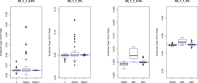
Empirical Type I error rates of the tests for the homoscedastic cases (All_1_1). All the results from the simulation study are combined. Left panel: (Semi-)parametric test empirical Type I error rates at α = 0.005 (left) and at α = 0.05 (right). Right panel: Nonparametric test empirical Type I error rates at α = 0.005 (left) and at α = 0.05 (right)

References
Algina, J., Oshima, T. C., & Lin, W.-Y. (1994). Type I error rates for Welch’s test and James’s second-order test under nonnormality and inequality of variance when there are two groups. Journal of Educational and Behavioral Statistics, 19(3), 275–291.
Amrhein, V., Trafimow, D., & Greenland, S. (2019). Inferential statistics as descriptive statistics: There is no replication crisis if we don’t expect replication. The American Statistician, S1(73), 262–270.
Baker, M. (2016). Is there a reproducibility crisis? A Nature survey lifts the lid on how researchers view the’crisis rocking science and what they think will help. Nature, 533(7604), 452–455.
Begg, C. (2020). In defense of p values. JNCI Cancer Spectrum, 4(2).
Benjamin, D. J., Berger, J. O., Johannesson, M., Nosek, B. A., Wagenmakers, E.-J., Berk, R., ..., Johnson, V. E. (2018). Redefine statistical significance. Nature Human Behaviour, 2, 6–10.
Berry, D. (2017). A p-value to die for. Journal of the American Statistical Association, 112(519), 895–897.
Bono, R., Blanca, M., Arnau, J., & Gómez-Benito, J. (2017). Non-normal distributions commonly used in health, education, and social sciences: A systematic review. Frontiers in Psychology, 8(1602).
Bradley, J. V. (1978). Robustness? British Journal of Mathematical and Statistical Psychology, 31(2), 144–152.
Brunner, E., & Munzel, U. (2000). The nonparametric Behrens-Fisher problem: Asymptotic theory and a small-sample approximation. Biometrical Journal, 42(1), 17–25.
Chung, E., & Romano, J. P. (2013). Exact and asymptotically robust permutation tests. The Annals of Statistics, 41(2), 484–507.
Chung, E., & Romano, J. P. (2016). Asymptotically valid and exact permutation tests based on two-sample U-statistics. Journal of Statistical Planning and Inference, 168, 97–105.
Collins, F. S., & Tabak, L. A. (2014). NIH Plans to enhance reproducibility. Nature, 505(7485), 612.
Divine, G. W., Norton, H. J., Baron, A. E., & Juarez-Colunga, E. (2018). The Wilcoxon-Mann-Whitney procedure fails as a test of medians. The American Statistician, 72(3), 278–286.
Fagerland, M. W., & Sandvik, L. (2009). The Wilcoxon-Mann-Whitney test under scrutiny. Statistics in Medicine, 28, 1487–1497.
Field, A., Miles, J., & Field, Z. (2012) Discovery statistics using R. London: Sage Publications.
Fligner, M. A., & Policello, G. E. (1981). Robust rank procedures for the Behrens-Fisher problem. Journal of the American Statistical Association, 76(373), 162–168.
Galili, T., & Benjamini, Y. (2016). Its not the p-values fault - reflections on the recent ASA statement.
Gelman, A., & Robert, C. P. (2014). Revised evidence fo stastical standards. Proceedings of the National Academy of Sciences, 111(19), E1933.
Good, P. (2013) Permutation tests: A practical guide to resampling methods for testing hypotheses. Berlin: Springer-Verlag New York. See https://www.springer.com/gp/book/9781475732351.
Greenland, S. (2019). Valid p-values behave exactly as they should: Some misleading criticisms of p-values and their resolution with s-values. The American Statistician, 73(S1), 106–114.
Held, L. (2019). The assessment of intrinsic credibility and a new argument for p < 0.005. Royal Society Open, 6(181534).
Hirschauer, N., Grüner, S., Mußhoff, O., Becker, C., & et al. (2018). Pitfalls of significance testing and p-value variability: An econometrics perspective. Statistics Surveys, 12, 136–172.
Hirschauer, N., Grüner, S., Mußhoff, O., & Becker, C. (2019). Twenty steps towards an adequate inferential interpretation of p-values in econometrics. Journal of Economics and Statistics, 239(4), 703–721.
Ho, J., Tumkaya, T., Aryal, S., Choi, H., & Claridge-Chang, A. (2019). Moving beyond p values: Everyday data analysis with estimation plots. Nature Methods, 16(7), 565–566.
Holmes, C. (1983). Sample size in four areas of psychological research. Transactions of the Kansas Academy of Science, 86(2/3), 76–80.
Ioannidis, J. P. (2005). Why most published research findings are false. PLoS Medicine, 2(8), e124.
Janssen, A. (1997). Studentized permutation tests for non-iid hypotheses and the generalized Behrens-Fisher problem. Statistics & Probability Letters, 36(1), 9–21.
Janssen, A. (1999). Testing nonparametric statistical functionals with applications to rank tests. Journal of Statistical Planning and Inference, 81(1), 71–93.
Johnson, V. E. (2013). Revised standards for statistical evidence. Proceedings of the National Academy of Sciences, 110(48), 19313–19317.
Kelley, K., & Preacher, K. J. (2012). On effect size. Psychological Methods, 17(2), 137.
Krueger, J. I., & Heck, P. R. (2017). The heuristic value of p in inductive statistical inference. Frontiers in Psychology, 8(908), 1–16.
Lakens, D. (2013). Calculating and reporting effect sizes to facilitate cumulative science: A practical primer for t-tests and ANOVAs. Frontiers in Psychology, 4, 863.
Lazic, S. E. (2018). Four simple ways to increase power without increasing the sample size. Laboratory Animals, 52(6), 621–629.
Liberati, A., Altman, D. G., Tetzlaff, J., Mulrow, C., Gøtzsche, P. C., Ioannidis, J. P., ..., Moher, D. (2009). The PRISMA statement for reporting systematic reviews and meta-analyses of studies that evaluate health care interventions: Explanation and elaboration. PLoS Medicine, 6(7), e1000100.
Marmolejo-Ramos, F., & Cousineau, D. (2017a). Perspectives on the use of null hypothesis statistical testing. Part I: The mighty frames of scientific and statistical inference. Educational and Psychological Measurement, 77(3), 471–474.
Marmolejo-Ramos, F., & Cousineau, D. (2017b). Perspectives on the use of null hypothesis statistical testing. Part II: Is null hypothesis statistical testing an irregular bulk of masonry? Educational and Psychological Measurement, 77(4), 613–615.
Marmolejo-Ramos, F., & Cousineau, D. (2017c). Perspectives on the use of null hypothesis statistical testing. Part III: The various nuts and bolts of statistical and hypothesis testing. Educational and Psychological Measurement, 77(5), 816–818.
Marmolejo-Ramos, F., Elosua, M. R., Yamada, Y., Hamm, N. F., & Noguchi, K. (2013). Appraisal of space words and allocation of emotion words in bodily space. PLoS ONE, 8(12), 1–13.
McNutt, M. (2014). Reproducibility. Science, 343(6168), 229–229.
McShane, B. B., Gal, D., Gelman, A., Robert, C., & Tackett, J. L. (2019). Abandon statistical significance. The American Statistician, 73(sup1), 235–245.
Morris, T. P., White, I. R., & Crowther, M. J. (2019). Using simulation studies to evaluate statistical methods. Statistics in Medicine, 38(11), 2074–2102.
Neubert, K., & Brunner, E. (2007). A studentized permutation test for the non-parametric Behrens-Fisher problem. Computational Statistics & Data Analysis, 51(10), 5192–5204.
OSC (2015). Open Science Collaboration: Estimating the reproducibility of psychological science. Science, 349(6251), aac4716.
Pauly, M., Asendorf, T., & Konietschke, F. (2016). Permutation-based inference for the AUC: A unified approach for continuous and discontinuous data. Biometrical Journal, 58(6), 1319– 1337.
Pauly, M., Brunner, E., & Konietschke, F. (2015). Asymptotic permutation tests in general factorial designs. Journal of the Royal Statistical Society: Series B (Statistical Methodology), 77(2), 461–473.
Paxton, P., Curran, P. J., Bollen, K. A., Kirby, J., & Chen, F. (2001). Monte carlo experiments: Design and implementation. Structural Equation Modeling, 8(2), 287–312.
Peng, R. (2015). The reproducibility crisis in science: A statistical counterattack. Significance, 12(3), 30–32.
Pesarin, F., & Salmaso, L. (2010) Permutation tests for complex data: Theory, applications and software. New York: Wiley.
Rafi, Z., & Greenland, S. (2020). Semantic and cognitive tools to aid statistical science: Replace confidence and significance by compatibility and surprise. BMC Medical Research Methodology, 244(20).
Rosnow, R. L., & Rosenthal, R. (1989). Statistical procedures and the justification of knowledge in psychological science. American Psychologist, 44(10), 1276–1284.
Ruxton, G. D. (2006). The unequal variance t-test is an underused alternative to Student’s t-test and the Mann-Whitney U test. Behavioral Ecology, 17(4), 688–690.
Satterthwaite, F. E. (1946). An approximate distribution of estimates of variance components. Biometrics Bulletin, 2(6), 110–114.
Szucs, D., & Ioannidis, J. P. (2017). Empirical assessment of published effect sizes and power in the recent cognitive neuroscience and psychology literature. PLoS Biology, 15(3), e2000797.
Trafimow, D., Amrhein, V., Areshenkoff, C., Barrera-Causil, C. J., Beh, E. J., Bilgiç, Y., ..., Marmolejo-Ramos, F. (2018). Manipulating the alpha level cannot cure significance testing. Frontiers in Psychology, 9(699), 1–7.
Wasserstein, R. L., & Lazar, N. A. (2016). The ASA’s statement on p-values: Context, process, and purpose. The American Statistician, 70(2), 129–133.
Welch, B. L. (1947). The generalization of ‘Student’s’ problem when several different population variances are involved. Biometrika, 34(1/2), 28–35.
Wilcox, R. R. (2017) Introduction to robust estimation and hypothesis testing, (4th edn.) Cambridge: Academic Press.
Yoshimura, N., Yonemitsu, F., Marmolejo-Ramos, F., Ariga, A., & Yamada, Y. (2019). Ask difficulty modulates the disrupting effects of oral respiration on visual search performance. Journal of Cognition, 2(1), 1–13.
Zwaan, R. A., Etz, A., Lucas, R. E., & Brent Donnellan, M. (2018). Making replication mainstream. Behavioral and Brain Sciences, 41(e120), 1–61.
Acknowledgements
We would like to thank the Editor and Associate Editor for handling the manuscript in a timely manner. We would also like to thank two anonymous reviewers for their useful suggestions, which have led to substantial improvement in the quality of the article. Frank Konietschke was supported by DFG KO 4680/3-2 and Markus Pauly was supported by DFG PA 2409/3-2.
Author information
Authors and Affiliations
Corresponding author
Additional information
Open Practice Statement
None of the in-silico experiments (simulations) was preregistered.
Publisher’s note
Springer Nature remains neutral with regard to jurisdictional claims in published maps and institutional affiliations.
Rights and permissions
About this article

Cite this article
Noguchi, K., Konietschke, F., Marmolejo-Ramos, F. et al. Permutation tests are robust and powerful at 0.5% and 5% significance levels. Behav Res 53, 2712–2724 (2021). https://doi.org/10.3758/s13428-021-01595-5
Accepted:
Published:
Issue Date:
DOI: https://doi.org/10.3758/s13428-021-01595-5