


1. Introduction
Determination of avalanche runout distances is fundamental for avalanche hazard mapping in land-use planning. This is achieved with complementary methods and using sources of information, such as the identification of vegetation clues, historical and eyewitness information, dendrogeomorphological analysis and the analysis of aerial images as well as digital terrain models (DTMs) and derived maps (Oller and others, Reference Oller2015). The determination of avalanche runout distances becomes more complex in areas where historical information is not available and vegetation clues are lacking. Calculation models, complementary to the abovementioned sources and methods, are particularly useful tools in these situations. Usually, dynamic models, statistical models (including the so-called statistical α−β model) or a combination of both approaches are applied. Dynamic models generally provide information on velocity, flow height, impact pressure and runout distances, and are especially suitable for engineering purposes. The main limitation of these models is that the information, which is used to build them (e.g. snow volume and friction coefficients) is often estimated from a limited set of available data. Small variations in these parameters can lead to large differences in the runout distances calculated (Lied, Reference Lied1998; Ancey, Reference Ancey2006). α−β and statistical models determine the runout distance from the topographic parameters of the avalanche path, but are unable to determine the other fundamental parameters for engineering purposes.
The basic idea of the α/β and statistical models is that, having a sufficient number of well-known avalanche occurrences, relationships among the data can be found as correlations from the laws of probability. For avalanches, the models are constructed using objective topographic parameters of a representative set of avalanche occurrences whose runout distances are known. The obtained correlations can, then, be used as predictors (Ancey, Reference Ancey2006). Hence, statistical characterisation of extreme avalanche runout using simple topographic inputs is able to predict maximum runout distance (Delparte and others, Reference Delparte, Jamieson and Waters2008). The two most widely used models are (1) the α–β model (Lied and Bakkehøi, Reference Lied and Bakkehøi1980), a regression model that allows a deterministic prediction of the extreme runout to be expected in a given path, and (2) the runout ratio model (McClung and others, Reference McClung, Mears and Schaerer1989), a runout ratio or density function probability model that fits a Gumbel distribution to the runout avalanche data. Later, Keylock (Reference Keylock2005) proposed that the generalised Pareto distribution is a more appropriate one and since then it has been applied by other authors (e.g. Favier and others, Reference Favier, Eckert, Faug, Bertrand and Naaim2016). Eckert and others (Reference Eckert, Parent and Richard2007) proposed a method for computing the predictive distribution of snow avalanche runout distances based on Bayesian modelling, and Lavigne and others (Reference Lavigne, Eckert, Bel, Deschâtres and Parent2017) implemented geostatistics through a Bayesian hierarchical model to tackle the spatial dependence of avalanche runout altitudes. But, apart from the runout distance, these approaches are unable to determine the other fundamental parameters for engineering purposes. To overcome the limitations of these calculation methods, coupled statistic-dynamical approaches have been proposed (Eckert and others, Reference Eckert, Naaim and Parent2010). They are based on a dynamic model, probability distributions are chosen for the input variables and fictitious avalanches are generated using Monte Carlo simulations to study the variability of the outputs (Barbolini and Keylock, Reference Barbolini and Keylock1999; Bozhinskiy and others, Reference Bozhinskiy, Nazarov and Chernouss2001; Meunier and others, Reference Meunier, Ancey and Naaim2001; Maggioni, Reference Maggioni2004). Barbolini and Savi (Reference Barbolini and Savi2001) and Meunier and Ancey (Reference Meunier and Ancey2004) calibrated simple parametric models using the available local data to improve the input distributions that appropriately represent the variability of the avalanche phenomenon at the studied site. Ancey and others (Reference Ancey, Gervasoni and Meunier2004) developed a coupled, conceptual model that proposes a probabilistic method to deduce the relationship between the probability distribution of input and output variables on the used dynamics model. Eckert and others (Reference Eckert, Parent, Naaim and Richard2008) described a general Bayesian framework for computing return periods for avalanche hazard zoning; this allows local data to be used to perform on-site calibration of an avalanche propagation model and computation of design return periods, and Eckert and others (Reference Eckert, Naaim and Parent2010) expanded this approach by including a depth-averaged fluid propagation model with a Voellmy friction law in the same Bayesian stochastic framework.
In this context of model development, often, for solving a specific problem, experts will typically combine several of these methods in their analysis, weighting the estimates in which they have greater confidence. Thus, the application of α−β models is only one of the methods used for solving some avalanche problems (Jones and Jamieson, Reference Jones and Jamieson2004).
The current study builds on the α–β regression approach, based on a detailed extreme avalanche database to determine the runout distance of extreme avalanches solely as a function of topography. It is a simple statistical regression that explains observed runout distances using various topographic covariates. Therefore, this approach can be considered as a deterministic prediction of the extreme runout to be expected in a given path, and uncertainty considerations only concern statistical uncertainty related to sample size limitation. Despite its simplicity, the model is relatively successful for the prediction of extreme runout distances (Gauer and others, Reference Gauer, Kronholm, Lied, Kristensen and Bakkehoi2010). The model (where α represents the runout and β the main inclination of the avalanche track; see Section 3.1) was developed by Lied and Bakkehøi (Reference Lied and Bakkehøi1980) using data from 111 avalanche paths in Norway that had very well-defined runout distances. They found that β was the only significant predictor and, since then, the α–β model has been adapted to other mountain ranges in Europe, North America and Japan (Table 1).
Table 1. Comparison of the α–β runout models (general equations)
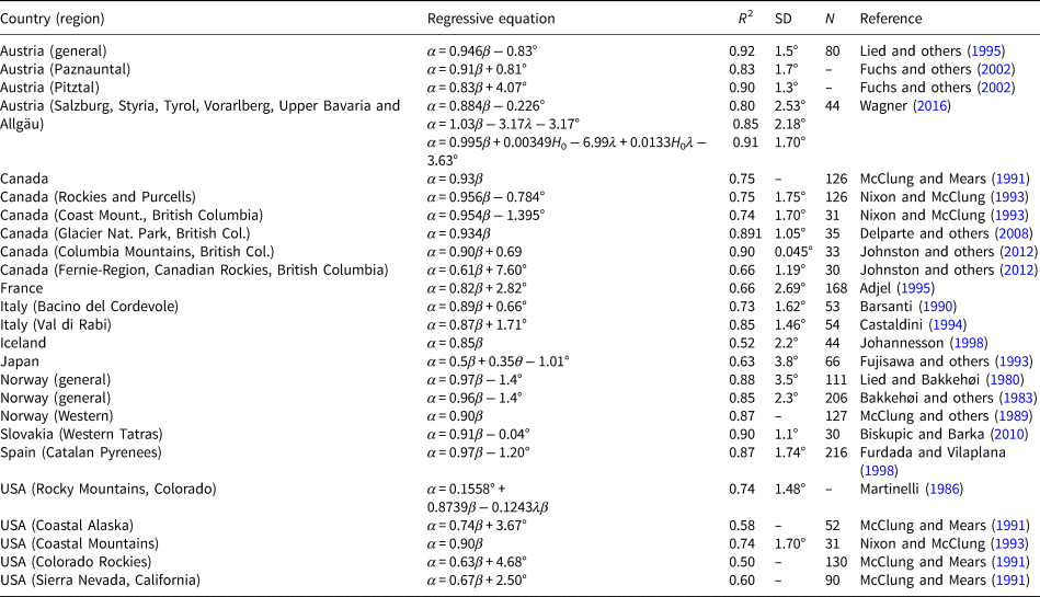
Completed and updated form Wagner (Reference Wagner2016). R 2, Pearson correlation coefficient; SD, standard deviation; N, number of paths used to obtain the model.
Using the equations of the obtained models, one can estimate the mean value of α for a given path. Assuming the residuals to be normally distributed, the mean can be assumed to approximate the median (50th percentile, non-exceedance probability p = 0.5; Jamieson, Reference Jamieson2018). By increasing p ($\hat{\alpha } = f( \beta ) -z_pSe$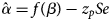 , were zp is the corresponding value of the normal distribution for a given non-exceedance probability p, and Se is the standard error of estimation for the regression), the probability of avalanches to exceed the predicted α is reduced.
Furdada (Reference Furdada1996) and Furdada and Vilaplana (Reference Furdada and Vilaplana1998) applied the α–β regression model for the first time in the Pyrenees. They used 1 : 50 000 topographic maps with 20 m contours (DTMs were still in development then). Avalanche data came from the first cartography campaigns being carried out in the western Catalan Pyrenees to provide information for the avalanche cadaster of Catalonia, the forerunner of the Avalanche Database of Catalonia (BDAC, Oller and others, Reference Oller, Marturià, González, Escriu and Martínez2005) that is presently maintained and updated by the Cartographic and Geological Institute of Catalonia (ICGC). Furdada and Vilaplana (Reference Furdada and Vilaplana1998) emphasised that the map scale of 1 : 50 000 was at the limit of the resolution required for this type of analysis (although it was the most accurate map scale at that time) and that there was a lack of knowledge about the occurrence of the avalanches in the dataset used for obtaining the model, which they estimated to be more than once in 30 years. They considered that their equations only provide an approximation of the runout on very poorly known avalanche paths, and do not contribute to improve the accurate mapping of the largest avalanches due to (1) the scale of the available topographical maps, (2) the relative small dimensions of the Pyrenean valleys and to (3) the dispersion of the residuals (α SD) likely due to the poor knowledge of the occurrence of the avalanches treated. The authors agreed with previous studies, such as that of McClung and Lied (Reference McClung and Lied1987), which indicated that the independent variable β was the one that best explained the dependent variable α. They also pointed out that the morphology of the topographic profile significantly influences the runout distance and obtained four regression models according to the topographic characteristics of the terrain profile. Furdada and Vilaplana (Reference Furdada and Vilaplana1998) recommended that for future studies, (1) the avalanche cadastre should be improved to provide more reliable data, (2) the accuracy of topographic bases should be improved and (3) DEMs should be used.
Since the study of Furdada (Reference Furdada1996), there have been important advances in digital cartography (e.g. topographic bases, high-resolution DEMs and digital orthoimagery). Furthermore, the knowledge of avalanche dynamics in the Catalan Pyrenees has also improved with the elaboration of the Avalanche Paths Map (Oller and others, Reference Oller2006), the implementation of the BDAC (ICGC; Oller and others, Reference Oller, Marturià, González, Escriu and Martínez2005) and a wider knowledge on the dynamics of major-avalanche cycles (Muntán and others, Reference Muntán2009; García and others, Reference García, Peña, Martí, Oller and Martínez2010; Oller and others, Reference Oller2015). On this basis, the current study updates the equations obtained by Furdada and Vilaplana (Reference Furdada and Vilaplana1998), because more accurate base information is now available.
The current study aimed to (1) update the α–β model for the Catalan Pyrenees, using the cartographic tools currently available and the latest knowledge on avalanche dynamics in this area, particularly the extreme-avalanche occurrences during the last period of ~100 years, (2) analyse the factors that influence the runout distance, taking into account the morphometric and dynamic characteristics of the avalanches of the dataset and (3) to investigate whether particular characteristics of the paths can have an influence on the fact that the extreme avalanches do not reach the β point, as is the case in 21% of the extreme avalanche occurrences in the dataset (see Section 3.2), and if on the other hand, the particular characteristics of the paths can influence the largest runout distances.
2. Study area
The study area corresponds to the Catalan Pyrenees, which is at the southeast of the Pyrenees mountain range (Fig. 1). It spans 130 km in the E–W axis and 50 km in the N–S axis. Elevations range from 600–1000 m in the valley bottoms to heights hardly exceeding 3000 m for the highest mountain peaks. The timberline varies between 2100 and 2500 m a.s.l. (Carreras and others, Reference Carreras1996). Three different climates have been identified (García and others, Reference García2007; Fig. 1). The northwestern part has a humid oceanic climate with regular winter precipitation. In winter, the total amount of snowfall is ~500–600 cm and the average temperature is −2.5°C at 2200 m a.s.l. Towards the south, the climate gains continental traits and winter precipitation decreases. In winter, the average new snow precipitation at 2200 m a.s.l. is 250 cm and the average temperature is −1.3°C. The prevailing winds are from the north and northwest, and they are more intense than in the oceanic region, often with gusts that are over 100 km h−1. In the eastern Pyrenees, the Mediterranean influence predominates. Winter precipitation increases but is irregularly distributed and is linked to Mediterranean cyclogenesis. In winter, the total amount of new snow at 2200 m a.s.l. is ~350–450 cm and the average temperature is −0.8°C. The prevailing winds come from the north and the strongest gusts often exceed 200 km h−1 at 2200 m a.s.l.
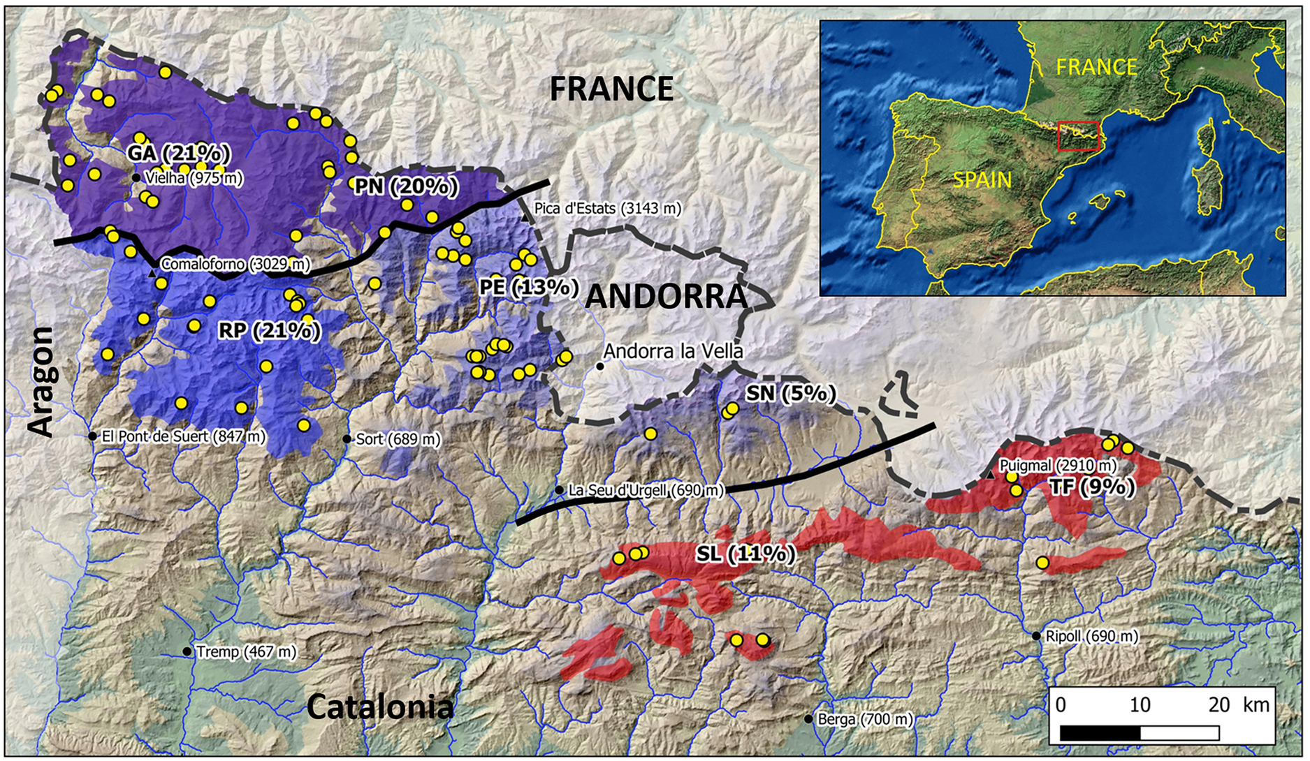
Fig. 1. Study area. The MANR are: GA (Garona), PN (Pallaresa Nord), RP (Ribagorçana-Pallaresa), PE (Pallaresa Est), SN (Segre Nord), SL (Segre-Llobregat) and TF (Ter-Freser). The coloured areas correspond to the areas susceptible to avalanche activity. MANRs with oceanic influence are shown in violet, MANRs in the transition zone are shown in blue and MANRs with Mediterranean influence are shown in red. The intensity of the colour indicates the frequency of MAE (% in brackets). Yellow dots correspond to the location of the paths with avalanche occurrences used in the current study.
Seven regions have been defined (Major Avalanche Nivological Regions, MANR) according to the frequency and spatial distribution of major avalanche episodes (MAE) or cycles (Oller and others, Reference Oller2015; Figure 1). The oceanic climate regions include Garona (GA) and Pallaresa Nord (PN). This climate produces the highest frequency of occurrence of MAEs, with northern and northwestern advections being the most frequent. The transition zone comprises the Ribagorçana-Pallaresa region (RP), Pallaresa Est (PE) and Segre Nord (SN). This area shows a decrease in the frequency of MAEs from W to E, SN having fewer MAEs. This large area is considerably influenced by advections coming from the north and northwest, combined with southern-southwestern advections. Finally, the area with the Mediterranean influence comprises Segre-Llobregat (SL) and Ter-Freser (TF). The frequency of MAEs is higher here than in SN, but the origin of the advections that generate MAEs is more varied and characteristically come from the east and southeast.
3. Materials and methods
3.1 The α–β model
The α–β model is based on a large number (>30) of runout positions of the so-called ‘extreme’ avalanche occurrences (avalanches with return periods of ~100 years). As these data originate from destructive avalanches, it is reasonable to assume that most of these occurrences correspond to dry-mixed avalanches, relatively large to their path, partially fluidised and accompanied by a powder cloud (Gauer, Reference Gauer2014) and therefore with similar behaviours (Lied and Bakkehøi, Reference Lied and Bakkehøi1980; McClung and others, Reference McClung, Mears and Schaerer1989; Gauer and others, Reference Gauer, Kronholm, Lied, Kristensen and Bakkehoi2010).
Lied and Bakkehøi (Reference Lied and Bakkehøi1980) recorded the maximum known extent for each avalanche path. They considered the frequency of occurrence of those avalanches near their maximum extent may be of the order of 1 in 100 years or lower. In general, authors considered the extreme runout positions with the same criteria (McClung and Lied, Reference McClung and Lied1987; Mears, Reference Mears1988; McClung and others, Reference McClung, Mears and Schaerer1989; Gauer and others, Reference Gauer, Kronholm, Lied, Kristensen and Bakkehoi2010; Wagner, Reference Wagner2016), or even occurring less than once in 100 years (Sinickas and Jamieson, Reference Sinickas and Jamieson2014), but bearing in mind that the true return period probably ranges from 30 to 300 years (Jones and Jamieson, Reference Jones and Jamieson2004; McClung and others, Reference McClung, Mears and Schaerer1989).
Lied and Bakkehøi (Reference Lied and Bakkehøi1980) obtained data of ten topographic parameters, identified through topographic maps, aerial images and fieldwork. In 1983 Bakkehøi and others extended the previous analysis by increasing the number of avalanche occurrences to 206 and adding new predictive variables. They found that the best equation to predict α was function of β and Hα (vertical drop of the avalanche path), and also included the parameters y″ (shape factor or curvature of the path) and θ (inclination of the starting zone; see next paragraph). Nevertheless, the only significant one was β. Nixon and McClung (Reference Nixon and McClung1993) obtained, with other combinations of parameters, similar results.
In Figure 2, the main parameters used for the derivation of the α–β model are plotted. Various combinations of H, β, θ and y″ have been used in regression models for estimating α around the world (Table 1). α (alpha angle, runout angle) is the inclination of the line connecting the upper end of the avalanche path with the maximum observed runout position (α point); α corresponds to the energy-line parameter defined by Heim (Reference Heim1932) to estimate the average coefficient of friction of a mass that moves from its initial position to its stopping position, being a measure of the energy dissipation along the path for each avalanche, and it was introduced as a simple measure of runout (Heim, Reference Heim1932; Scheidegger, Reference Scheidegger1973; Körner, Reference Körner1980). It may be used as a criterion or index for empirical avalanche reach (Lied and Bakkehøi, Reference Lied and Bakkehøi1980; McClung and Gauer, Reference McClung and Gauer2018). β (beta angle) is the inclination of the line connecting the upper point of the avalanche starting zone to the point of the topographic profile where the slope reaches 10° (β point, used by the model as a reference point). Gauer and others (Reference Gauer, Kronholm, Lied, Kristensen and Bakkehoi2010) included the condition that the corresponding β angle should be ≥15° in order to avoid unrealistically low β angles. The reason for using the β angle, or line, is to generate a simple, best description of the main inclination of the avalanche starting zone and track (Lied and Bakkehøi, Reference Lied and Bakkehøi1980; Bakkehøi and others, Reference Bakkehøi, Domaas and Lied1983; Gauer and others, Reference Gauer, Kronholm, Lied, Kristensen and Bakkehoi2010). Even though in early studies it was thought that 10° represents the transition zone between the track and the runout zone for large, dry-mixed avalanches, which start to slowdown and begin depositing at 10° (de Quervain, Reference De Quervain1972; Buser and Frutiger, Reference Buser and Frutiger1980), it is certainly not the case (Gauer and others, Reference Gauer, Kronholm, Lied, Kristensen and Bakkehoi2010; Sovilla and others, Reference Sovilla, McElwaine, Schaer and Vallet2010; Gauer, Reference Gauer2014, Reference Gauer2018). Almost all dry-mixed avalanches start to decelerate farther upslope (Gauer and others, Reference Gauer, Kronholm, Lied, Kristensen and Bakkehoi2010). θ (theta angle) corresponds to the slope of the upper 100 m of the starting zone (θ 100, Bakkehøi and others, Reference Bakkehøi, Domaas and Lied1983). Some studies consider the lower end of the starting zone to be the point where the slope reaches 28° (Lied and Toppe, Reference Lied and Toppe1989; Furdada and Vilaplana, Reference Furdada and Vilaplana1998). Recently, Wagner (Reference Wagner2016) applied θ 100, but reducing the length of the measurement if the 25° point was in between the upper 100 m. y″ is the second derivative of the polynomial function that better fits the terrain profile. It is a shape factor that describes the whole profile (Bakkehøi and others, Reference Bakkehøi, Domaas and Lied1983). The second-degree polynomial function is of the type: y = ax 2 + bx + c and, as previously described by other authors (e.g. McClung and Lied, Reference McClung and Lied1987); this polynomial provided an excellent fit to the avalanche terrain profiles, obtaining determination coefficients (R 2) >0.99. H is the vertical drop, measured as the difference between the upper end of the avalanche path at the y intercept and the minimum point on the second-degree polynomial function where y′ = 0. In general, it is assumed that H is very close to the vertical drop of the avalanche (Hα), and both values are assimilable given the proximity to the real slope of the avalanche path (McClung and Lied, Reference McClung and Lied1987). Hβ is the corresponding vertical drop measured between the upper end of the avalanche path at the y intercept and the β point. L is the horizontal length of the avalanche path from the starting point to α point. Lβ is the corresponding horizontal length from the starting point to β point.

Fig. 2. Main parameters of the α–β model (after Lied and Bakkehøi, Reference Lied and Bakkehøi1980).
In general, avalanche occurrences considered by most authors had a minimum vertical drop of 350 m, a terrain profile with little or no run-up or irregularities in the runout area, a differentiated and unique starting zone, and no anthropogenic modifications.
McClung and Lied (Reference McClung and Lied1987) and Nixon and McClung (Reference Nixon and McClung1993) found that short slopes (<350 m vertical drop) tend to run proportionately farther than larger slopes, and therefore the models developed for particular mountain ranges using the α–β runout method may not be applicable to short slopes, and that a particular need was the analysis of short avalanche paths with a vertical drop minor than 350 m. Jones and Jamieson (Reference Jones and Jamieson2004) developed a regression model specifically for short slopes in Canada. However, Wagner (Reference Wagner2016) investigated 49 avalanche occurrences in Austria some of which with drop heights <300 m and found that the model still works also for those drop heights.
The α–β model is not intended to include run-up. In contrast to the study of Lied and Bakkehøi (Reference Lied and Bakkehøi1980) and Bakkehøi and others (Reference Bakkehøi, Domaas and Lied1983), as part of the calibration of the model of the Austrian alpine region (Lied and others, Reference Lied, Weiler, Bakkehøi and Hopf1995), avalanches reaching small run-ups were also considered for the first time. Delparte and others (Reference Delparte, Jamieson and Waters2008) included avalanches with a maximum observed runout that involved a run-up the opposing slope of <25 vertical meters, from the valley bottom up to the recorded stopping point. They considered that in the avalanche paths that do run up the opposing slope <25 vertical meters, this difference is lessened as the winter progresses and the deposition of snow fills the depression and reduces the run-up amount. In their research, all the paths that include some run-up had measured run-up that accounted for <2.5% of their total vertical drop. In the current study, we have applied the same criteria.
Considering the use of DEMs, Delparte and others (Reference Delparte, Jamieson and Waters2008) demonstrated that variations in DEM resolution (5–25 m horizontal resolution) did not significantly affect α–β regression equations.
3.2 The avalanches’ database
Extreme avalanche occurrences used in the current study were extracted from the Major Avalanches Database (MADB), which stores major avalanche (MA) data (avalanches that exceeded the size of usual avalanches; Schaerer, Reference Schaerer1986) or destructive avalanche data (Laternser and Schneebeli, Reference Laternser and Schneebeli2002). As defined in Gauer (Reference Gauer2018), ‘major avalanches’ are avalanches that can be considered as R4, large relative to the path, or R5, major or maximum relative to the path (Greene and others, Reference Greene2016, 3.6.5.2. Size-relative to the path). Information collected in this database comes from the BDAC managed by the ICGC, whose sources of information and characteristics are described in detail in Oller and others (Reference Oller2015), as well as from additional research performed by the authors. The MADB includes the release date, snow and weather conditions, morphometries, flow characteristics and the damage caused by these major avalanches. This information was obtained from 30 years of avalanche observations (winter surveillance), photointerpretation (orthoimages available from 1946 to present), dendrogeomorphology (covering approximately from 1800 to present; Muntán and others, Reference Muntán, Andreu, Oller, Gutiérrez and Martinez2004, Reference Muntán2009, Reference Muntán, Oller, Gutiérrez and Stoffel2010), eyewitnesses (20th century mainly) and historical data (since 15th century). Currently, the MADB stores information on 897 major avalanches (MA), mapped in 551 avalanche paths. Only one avalanche occurrence per path was selected and it was considered to be the largest in, at least, 100 years (see next paragraph). The quantity and good quality of the information available enabled us to apply some constraints in the selection of the data (discussed below) used to obtain the best possible model.
MA occurrences since the end of the 19th century were classified by comparing the distribution of the runout distances in each avalanche path (Oller and others, Reference Oller2015) and selecting the largest one. In a few of the avalanche paths it is known from historical documents that avalanches occurred before the 19th century. These occurrences were considered not to correspond to the same set and were discarded. The reason was that all these avalanches occurred during the Little Ice Age (LIA; from 1300 to the end of 1800s; Mann, Reference Mann2002; Oliva and others, Reference Oliva2018). This climatic period, different to the present one and characterised by cycles with large temperature falls and considerable increases in precipitation, had increased numbers of severe catastrophic meteorological-related phenomena (e.g. floods, strong snowfalls, sea storms, persistent rain and droughts). In Catalonia, a concentration of catastrophic floods was identified during the periods 1580–1620, 1760–1800 and 1840–70 (Barriendos and Martín Vide, Reference Barriendos and Martín Vide1998; Barriendos and Llasat, Reference Barriendos and Llasat2003; Llasat and others, Reference Llasat, Barriendos, Barrera and Rigo2003; Blöschl and others, Reference Blöschl2020). All the avalanches occurring during these periods, therefore, probably occurring under climatic conditions that are different to the present conditions, as it has been described in 1888 snow avalanche cycle in the Spanish Cantabrian Mountains (García-Hernández and others, Reference García-Hernández, Ruiz-Fernández, Sánchez-Posada, Pereira and Oliva2018) or in 1803 and 1855 snow avalanche cycles in the Pyrenees (García and others, Reference García, Rodés, Gavaldà, Martí and Barriendos2005; Oller and others, Reference Oller, Fischer and Muntán2020), were separated from the dataset.
The goal of the α–β method is to work with ‘extreme’ occurrences. However, the α angles measured in this work are determined from the distal (downslope end) of the individual avalanche deposits or effects and not necessarily for maximum runout positions for the paths, that is, in a similar way that McClung and Gauer (Reference McClung and Gauer2018) do and point out in their work. This means that the dataset includes both, dense flow and powder runouts, probably from dry-mixed avalanches, as explained in Section 3.1. Given the uncertainty of the available data, the return period is likely to vary from 30/50 to 300 years, introducing unavoidable random variation in the data (McClung and Mears, Reference McClung and Mears1991). Besides, Mears (Reference Mears1992) considers that when many 50 to 200-year-old trees are destroyed by an avalanche, this damage provides convincing evidence that the avalanche has, about, an estimated return period of 100 years. In our study, considering the characteristics of the data in the MADB, we decided to work with well-estimated avalanches whose occurrence has been the largest in 100 years, or ‘extreme’ occurrences henceforth.
For the determination of the extreme occurrences, photointerpretation was essential. The ICGC website contains orthoimages of 18 flights covering the whole of the Catalan Pyrenees from 1946 to the present (1946, 1956, 1990, 1993, 1996/97, 2003, 2005, 2007, 2008, 2009, 2011, 2012, 2013, 2014, 2015, 2016, 2017 and 2018). This enables the state of the forest to be compared and analysed between 74 years ago and now. A well-developed forest in 1946 indicate a minimum previous period of 30 years necessary for its development without disturbances (in dendrogeomorphologycal research of several avalanche paths, the age of the oldest-affected trees was more than 200 years; Muntán and others, Reference Muntán, Andreu, Oller, Gutiérrez and Martinez2004, Reference Muntán2009, Reference Muntán, Oller, Gutiérrez and Stoffel2010). The identification of a major subsequent destructive avalanche through the identification of a new path in the forest, together with the analysis of the occurrences recorded in the same avalanche path, can be used to qualify this occurrence as extreme in 100 years. In our database, for avalanche paths with information from winter surveillance, eyewitness accounts, historical data or dendrogeomorphological analysis, the time window is longer. In any case, we can affirm that the extreme avalanches considered in this study were the largest occurrences at least in 100 years in their corresponding avalanche path.
The selected avalanches had to meet the necessary requirements for the α–β method, i.e. a differentiated and unique starting zone and no anthropogenic modifications (Sinickas and Jamieson, Reference Sinickas and Jamieson2014). The goal was to work with very well-defined individual and unmodified avalanche paths. This reduced the number of avalanches in the dataset used to 97 avalanche occurrences (12% of the dataset homogeneously distributed in the study area; Fig. 1).
The mapping of the avalanches was performed using the orthoimages described above, on the ICGC 1 : 5000 topographic map with 5 m contour distances, and a 5 m × 5 m DEM. The β point was placed on the topographic map at the point where the slope between the contours falls below 10°. In avalanche paths where the slope oscillates ~10°, benches shorter than 3% of Lβ (Fig. 2) were ignored during the selection of the β point because, according to Sinickas and Jamieson (Reference Sinickas and Jamieson2014) judgement and field experience, they are considered negligible compared to the length of the path. For benches larger than the 3% limit, other path characteristics were used to inform the decision based on expert criteria, as also applied by Furdada and Vilaplana (Reference Furdada and Vilaplana1998).
During the preparation of the data, we realised that not all the selected extreme avalanches reached the β point, with 20 avalanches (21%) in our dataset not reaching it. Other studies have also reported similar cases, as the pioneer one of Lied and Bakkehøi (Reference Lied and Bakkehøi1980), who found that 25% of the well-known avalanches that they used did not reach the β point. As they fitted the observed runout of the avalanches by linear regression, it is reasonable to assume that the error around the fit is approximately normal distributed (it has to be therefore expected that at least ~16% of the observed avalanches do not reach β). In order to distinguish the most extreme (smallest) α angle of each single avalanche, which might be regarded as a random variable and the expected value according to the regression model, in Section 4.2 the parameters that can explain these differences are explored.
For the selected avalanches, in addition to the morphometric parameters that were formerly used to evaluate α : β, H, L, y″ and θ (Lied and Bakkehøi, Reference Lied and Bakkehøi1980; Bakkehøi and others, Reference Bakkehøi, Domaas and Lied1983) (Fig. 2), we measured other parameters that are also considered to affect runout distances (Table 2).
Table 2. Descriptive statistics of the main topographic and morphometric parameters considered, and the correlation between the response variable α and the predictor variables used to develop the α–β model

N, number of paths where the variable was measured; SD, standard deviation; R 2, Pearson coefficient of determination; p-value, statistical significance. The variables that show the best correlation with α are highlighted in bold.
The variables H and L were substituted by Hβ and Lβ because when applying the regression analysis in an unknown avalanche path, only these variables can be measured (H and L are unknown). The topographical profiles (PTs) were classified according to the topography of the transition track – runout zones in order to group some usual shapes that can be classified similarly by different experts as (1) gradual: the slope of the track-runout zones decreases gradually; (2) abrupt: there is an abrupt transition from a relatively steep slope to a slope at or near 0° in the runout zone (hockey-stick, Jones and Jamieson, Reference Jones and Jamieson2004); (3) run-up: there is an abrupt transition from a relatively steep slope to a negative slope; (4) gradual/abrupt run-up: there is a gradual or abrupt transition ending in a negative slope and (5) complex (irregular): the slope in the transition track-runout is irregular (e.g. rocky bars and mounds). The area of the starting zone (Azs) of each avalanche path was measured on the horizontal projection. The area was defined by the highest estimated elevation of the starting zone, an average width, and for the lower side, the elevation where the slope decreases below 28°, or where the morphology of the terrain suggested it (e.g. confinement and cliffs). The mean aspect of the starting zone (Ozs) of each avalanche path was measured in degrees. Confinement (Con) was determined by measuring the % of the horizontal length (L) of the avalanche, confined. It was considered as confined, a relation width/depth of the channel <10. The climate region (Cli) in which the avalanche path is located (also considered by Lied and Bakkehøi, Reference Lied and Bakkehøi1980; Furdada and Vilaplana, Reference Furdada and Vilaplana1998; Jones and Jamieson, Reference Jones and Jamieson2004) was assigned to: (1) oceanic, (2) transition or (3) Mediterranean (Fig. 1). Another parameter that could affect avalanche runout distances is the area of the forest devastated by the avalanche, since this was an important area affected by many of the registered avalanche occurrences. The deforestation was measured by comparing aerial images before and after the avalanche occurrence. Although it was only possible to survey 24 cases, two variables were measured according to Anderson and McClung (Reference Anderson and McClung2012): the length of the deforested track (Def) was determined by measuring the percentage of the horizontal length of the avalanche, deforested. The horizontal distance to forest penetration (L_For) was measured from the highest point of the starting zone until the beginning of the forest.
Table 2 presents the descriptive statistics of each parameter, as well as the Pearson coefficient of determination (R 2) and the statistical significance (p-value) of the correlation of each variable with α.
4. Analysis and results
4.1 Application of the α–β runout model
In order to know the variables that may influence the runout of the avalanche (α) and their weight, a prediction model was performed by using multiple linear regression. Previously, all partial bivariate correlations between the dependent variable (α) and the independent variables of the terrain that have an influence on the runout distance (Table 2) were carried out. Every variable was tested for normal distribution using the Kolmogorov–Smirnov test at 5% confidence level. Not normally distributed variables were normalised through log-transformation. Thus, to know the association between α and the rest of the independent variables of continuous quantitative scale, the Pearson correlation (for those that follow a normal or parametric distribution) and a rho of Spearman (for those non-parametric) was performed. From the results obtained from the bivariate correlations, the variables associated with α with levels of statistical significance >0.05 were included in the multiple linear regression model.
Given the limited size of the dataset, a general model was constructed with 83 avalanche occurrences. From the initial dataset (97 avalanche occurrences), 14 avalanches (15% of the dataset) were separated randomly (one of every seven avalanches was selected according to its position listed by its code) to check the reliability of the model and validate it later.
The multiple regression model was derived from the variables β, Azs (log) and Lβ, all of them associated with α, with levels of statistical significance >0.05, and very significant for the function with p-values <0.001; for all the other measured parameters, the correlation was very poor (Tables 2 and 3). The non-standardised B (beta) regression coefficients are positive for the β and Lβ variables (Table 3). Thus, when increasing the value of the β and Lβ variables, the α value increases. The negative value of the B coefficient for the variable Azs (log) indicates an inverse association with the α variable. The standardised function coefficients help to determine the weight or influence of each of the variables included in the model. Thus, the β variable, with a value of 0.923 (standardised coefficient), is the one that shows the most influence on the runout of the avalanches through the α variable
Table 3. Coefficients of the multiple linear regression model with three variables

B, beta non-standardised correlation coefficient; SD, standard deviation; t, t statistic; p-value, statistical significance; CI, confidence interval; VIF, variance inflation factor.
The goodness of the fit of the regression model to the observed data has been checked using the coefficient of determination (R 2). The latter indicates that the percentage of variance explained by the regression line of the model is 81%. When applying the Fisher's test, by means of the analysis of variance (ANOVA), the result with a significance value of <5% confirms the goodness of the obtained model. The confidence interval (CI) at 95% is precise enough for each one of the function coefficients, confirming the robustness of the model. The values of tolerance (percentage of variance not explained by other predictors) is >0.65, with VIF values (variance inflation factor) lower than 2, thus so weak that collinearity of the explanatory variables can be considered inexistent and doesn't affect the results (Thompson and others, Reference Thompson, Kim, Aloe and Becker2017).
Finally, an analysis of the residuals was performed, which confirmed that the basic assumptions of normality and non-existence of heteroscedasticity were met. For the diagnosis performed on the goodness of the fit and the analysis of the residuals, it can be confirmed that the model is good and robust.
Equation (1), obtained by multiple linear regression is:

The model was then applied to the 14 avalanche occurrences selected to check their reliability. The values obtained were located within the 95% CI (Fig. 3, blue dots), indicating a satisfactory fit of the model.
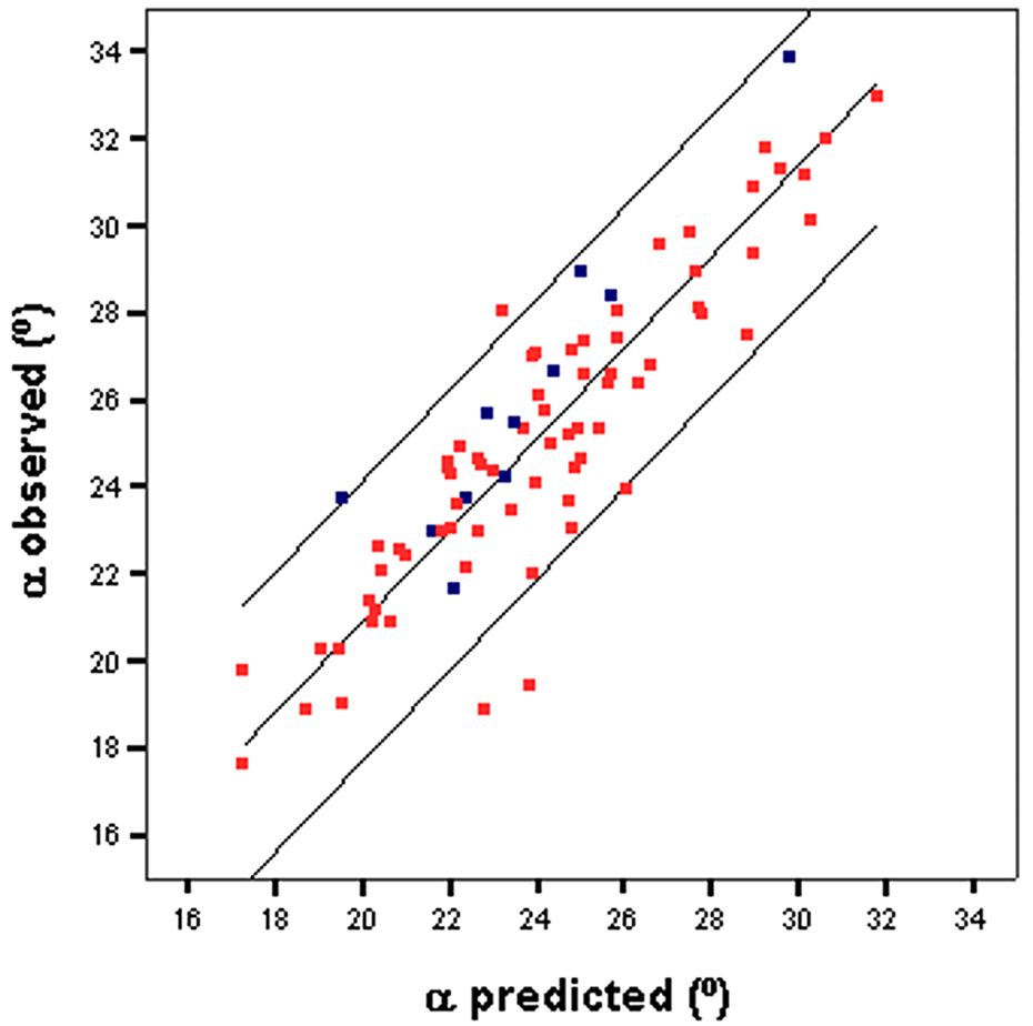
Fig. 3. Plot of the observed α values with respect to those obtained with regression Eqn (1). The outside lines indicate the 95% confidence bands. Red dots: training sample (to construct the model); blue dots: test sample (to validate the model).
In Table 4, descriptive statistics of α and error (α observed − α predicted) values obtained after applying to the 97 extreme avalanches Eqn (1), and those obtained by Furdada and Vilaplana (Reference Furdada and Vilaplana1998) and Oller and others (Reference Oller, Baeza and Furdada2018) are shown. Using the general equation obtained by Furdada and Vilaplana (Reference Furdada and Vilaplana1998; α = 0.97β − 1.20°, R 2 = 0.87, SD = 1.74°, N = 216), we obtained the same mean α angle (24.7°) as the one obtained with our own equation.
Table 4. Descriptive statistics of α predicted and error (α observed − α predicted) values obtained after applying to the 97 extreme avalanche occurrences Eqn (1), and those obtained by Oller and others (Reference Oller, Baeza and Furdada2018) and Furdada and Vilaplana (Reference Furdada and Vilaplana1998), respectively; Eqn (1) is more accurate (lower error values)

Oller and others (Reference Oller, Baeza and Furdada2018) obtained a model (α = 0.85β + 2.10°, R 2 = 0.76, SD = 1.87°, N = 63) by censoring a dataset similar to the one used in the current study, although not including the avalanches that did not reach the β point, as Furdada and Vilaplana (Reference Furdada and Vilaplana1998) did. In spite of this, results are quite similar (α and error values, Table 4). Hence, Eqn (1) would be recommended to estimate runout distances for avalanche return periods of the order of 100 years, in this region, like the one obtained by Furdada and Vilaplana (Reference Furdada and Vilaplana1998).
As a broader exercise of regression equations comparison, the results of our Eqn (1) were compared with the results obtained when applying other equations from other mountain chains to our avalanche occurrence dataset. In Figure 4, the descriptive statistics of error and α angle obtained with equations (1 to 11) from Table 1 are plotted. Equations are ordered from lower (left) to higher (right) mean α error, being 1, the equation obtained in this research (Table 3). It can be observed that the mean value of the error increases as the mean value of α decreases, although some error values are close to those in Eqn (1) (Canada, 2; France, 3; Norway, 4; Japan, 5; Austria, 6). The dispersion, however, is much greater, and especially in Japan (5). With the exception of Canada (2) and France (3), the mean α values obtained are lower than that obtained with other equations, especially from Slovakia (7) to the right side of the graph. Despite the exception of Canada (2) and Norway (4), in general in continental regions and at higher latitudes, the mean α angles are smaller (longer runout, right sector of the graph), and in maritime regions and at lower latitude α angles are higher (shorter runout, left side of the graph).
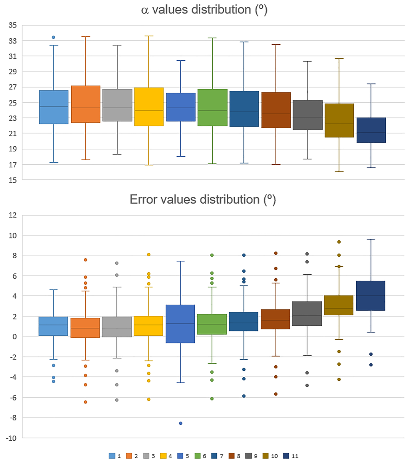
Fig. 4. Boxplots of α predicted and error values obtained after applying to the 97 extreme avalanche occurrences the general equations listed in Table 1, ordered in increasing order of mean error (from left to right). 1, Eqn (1); 2, Canada (McClung and Mears, Reference McClung and Mears1991); 3, France (Adjel, Reference Adjel1995); 4, Norway (Lied and Bakkehøi, Reference Lied and Bakkehøi1980); 5, Japan (Fujisawa and others, Reference Fujisawa, Tsunaki and Kamiishi1993); 6, Austria (Lied and others, Reference Lied, Weiler, Bakkehøi and Hopf1995); 7, Slovakia (Biskupic and Barka, Reference Biskupic and Barka2010); 8, USA Coastal Mountains (Nixon and McClung, Reference Nixon and McClung1993); 9, USA Coastal Alaska (McClung and Mears, Reference McClung and Mears1991); 10, Iceland (Johannesson, Reference Johannesson1998); 11, USA Colorado Rockies (McClung and Mears, Reference McClung and Mears1991).
4.2 Analysis of the extreme values obtained
To study the variables that influence a greater or lower runout of the avalanches (i.e. that exceed or do not reach the α predicted), a comparative analysis of the data was performed. As a first step, the data were grouped into two sets. From the dataset, 64 (66%) avalanche occurrences had a positive error (the observed runout was shorter than that predicted by the model) and 33 (34%) avalanche occurrences had a negative error (the observed runout was longer than that predicted by the model). This suggests that the model tends to favour longer runout distances. The end values of the distribution (positive or negative values beyond a SD, 25 and 8 avalanches, respectively) were separated in order to highlight main differences between the extreme values of the avalanche dataset. The 20 avalanche occurrences not reaching the β point were included in the 25 positive occurrences group (Table 5). No differences were found between independent datasets based on T, Mann–Whitney or ANOVA tests, according to the types of variables analysed.
Table 5. Descriptive statistics of the main topographic and morphometric parameters of the avalanches with positive error >1 SD (observed avalanches don't reach predicted runout distances) and negative error <−1 SD (observed avalanches exceed predicted runout distances)
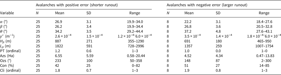
Analysing comparatively the parameters corresponding to each population, despite the reduced number of cases of the two datasets, there are some differences to be mentioned. On the one hand, for a similar mean β angle (between 26° and 27°), α angles are logically lower for avalanches with a negative error (larger runout). On average, avalanches with a positive error are larger (larger Hβ, Lβ and Azs) than the one's with a negative error. The mean aspect of the starting zone of the avalanches with positive error is NW, whereas for avalanches with a negative error is SE (Table 5). No tendencies were found in relation to climate divisions.
5. Discussion
5.1. Considerations about the obtained model
Our update of the α–β model for the Catalan Pyrenees has produced a general equation with three significant variables. The parameters of the model (variance, tolerance and CI) confirm its robustness, with a coefficient of determination R 2 = 0.81. The 97 avalanches of the dataset took place mainly during the 20th century, under climatic conditions that are similar to current conditions. Therefore, the equation provides estimates of the runout distances for avalanches occurring about once in 100 years. If the SD is subtracted, the non-exceedance probability factor increases, providing a boundary to the uncertainty.
Gauer and others (Reference Gauer, Kronholm, Lied, Kristensen and Bakkehoi2010) found that there was neither volume nor fall height dependency with runout. However, Eqn (1) shows a slight relation with Lβ (horizontal length of the avalanche until β point), and Azs, an indirect measure of the size of the avalanche at the starting zone, result that conceptually contradicts the results obtained by these authors. They explained that erosion and entrainment of snow seem to be crucial for avalanches to reach long runout distances, which feed and grow through snow entrainment at the head of the avalanche, but long runouts are not dependent on the total mass. In our case, we have not considered entrainment and neither avalanche mass at the starting zone or runout zone, because they are not parameters that can be directly derived from the topography of the path. We used indirect variables of the size of the avalanche (Lβ and Azs) which counteract: larger Azs provide longer runouts and larger Lβ provide shorter runouts. This result may be explained because the longer is the track, the longer act the frictional forces (approximately when slope decrease below 24°, Gubler and others, Reference Gubler, Hiller, Klausegger and Sutter1986; McClung and Mears, Reference McClung and Mears1995), and also the higher are the friction forces due to channelisation, roughness (forest and terrain) and densification of the flow (Bakkehøi and others, Reference Bakkehøi, Domaas and Lied1983), especially for dense flow avalanches (Wagner, Reference Wagner2016). This can be related to shorter slopes tendency to provide larger runouts compared to longer slopes, as explained in Section 3.1. In relation to the area of the starting zone, the largest it is, the longer is the runout because of the higher mass incorporated, involving the size effect indicated by Pudasaini and Hutter (Reference Pudasaini and Hutter2007). Thus, the larger is the avalanche, the higher may be its capacity of snow erosion and entrainment.
5.2. Comparison with the former model
The equation obtained (1) provide similar runout distances than those obtained more than 20 years ago by Furdada and Vilaplana (Reference Furdada and Vilaplana1998). Furdada and Vilaplana (Reference Furdada and Vilaplana1998) reported that the results obtained with their equations were probably undervalued given the uncertainty about the return period of the avalanches in the dataset, estimated higher than 30 years. As the goal was to register extreme avalanches, only avalanches that surpassed the β point were registered, with the damage caused by past avalanches in the forest and eyewitness information being the main criteria used to identify these runout distances. Therefore, according to the dataset, the Furdada and Vilaplana (Reference Furdada and Vilaplana1998) equation should provide more conservative results, that is, lower α angles than for a non-censored dataset. However, the results were likely to correspond to avalanches that include some more frequent ones, given that the model produced similar runout distances despite the use of a censored dataset, and some few less frequent and rarer ones. Compared to the dataset used in the current study, which considers avalanche occurrences of the order of 100 years return period, including all avalanches, reaching and not reaching the β point (non-censored dataset), the dataset used by Furdada and Vilaplana (Reference Furdada and Vilaplana1998) should correspond to a lower return period, as they also suggested. Their high coefficient of determination (R 2) value (0.87) was probably due to a more homogeneous dataset, by not including avalanches not reaching β. Therefore, despite obtaining similar results, the datasets used in both studies had significant differences, that can be due to: (1) a different criterion in the selection of the avalanche occurrences that feed the model (i.e. censoring of avalanche occurrences not reaching the β point); (2) the smaller geographic area involved in the former analysis (only western Catalan Pyrenees, in the oceanic and western transition climatic areas that have a higher MAE – major avalanche episode or cycle – frequency, Fig. 1; see next section) and (3) a less precise mapping tools.
Furdada and Vilaplana (Reference Furdada and Vilaplana1998) obtained four regression models according to the topographic characteristics of the terrain profile. In our dataset, neither y″, the shape factor that describes the terrain profile, nor PT, a classification of the terrain shape at the transition track-runout zones, had statistical significance with the variable α. Probably, the dataset was not large enough to include a statistical significant number of cases for each shape class.
5.3. Terrain and climate influence on extreme runouts
When analysing the avalanches with the most extreme positive and negative error, certainly there is not a clear distribution in function of climate divisions, but there are differences related to topography of the avalanche paths as McClung and others (Reference McClung, Mears and Schaerer1989) indicate.
The variables that have the most influence on extreme runout, above and below α obtained by the model, are the variables related to the size (Lβ, Hβ and Azs) and the aspect of the starting zone, Ozs (Table 5). Smaller and SE facing starting zones provide longer runouts than expected, for more than 1 SD. In relation to the aspect of the starting zone (Ozs), negative values (larger runout) are associated with SE starting zones and positive values (shorter runout) are associated with NW starting zones. In SE starting zones runout distances are larger than predicted. This can be explained by the highest frequency of cold NW advections (Oller and others, Reference Oller2015) which accumulate drifted snow towards SE starting zones, produce storm slabs and generate cold dry snow avalanches within southern slopes. The atmospheric patterns that generate avalanches in northern slopes are less frequent and involve warmer conditions and this may explain why there are more avalanches with a runout shorter than predicted. Forest extent in these avalanche paths is larger due to a less avalanche activity and it offers a higher roughness to the flow to extreme avalanches. The available information on forest destroyed by the avalanches of the dataset indicates that in northern slopes the mean deforested area per avalanche is 3.59 ha and in southern slopes is 2.23 ha, which supports this hypothesis. In SE facing avalanche, paths with a negative error (larger runout), starting zones are smaller. This would be explained by the increase of the snow mass released because of the wind loading contribution in these starting zones.
This result becomes very relevant in terms of uncertainty. When applying the model, the subtraction of 1 SD corresponds to a non-exceedance probability of p = 0.84, which means that 84% of the paths should have runouts that do not exceed the predicted α, which is a high security range. In consequence, in avalanche paths with such characteristics (starting zones smaller and facing SE) it would be recommended to land-use planners to consider increasing the non-exceedance probability.
5.4. Comparison with other models
Regarding the exercise of comparison of the model obtained in this study and other models, some constraints and considerations arise. The first, obvious one is that the database of avalanche occurrences affects the obtained equation and the consequent results. As an example, in the Catalan Pyrenees, censored (Oller and others, Reference Oller, Baeza and Furdada2018) and non-censored (this study) databases can generate mean similar results, but censored database ultimately produce a range of more conservative runouts and a range of larger errors (Table 4), resulting in a more imprecise estimation of the runouts.
The comparison of the results obtained with Eqn (1), with other equations obtained in other mountain ranges around the world (Fig. 4), shows how in the Pyrenees runouts are shorter, but relatively close to other European Alpine countries (e.g. the equation obtained from France could be applied to the Catalan Pyrenees, even though the SD error is larger). Results seem to show some climate influence: in general, in continental regions and at higher latitudes, the mean α angles are smaller (longer runout), and in maritime regions and at lower latitude α angles are higher (shorter runout). McClung and others (Reference McClung, Mears and Schaerer1989) considered that climate regime does not have a strong influence on extreme runouts on a time-scale of more than ~100 years. According to their experience, large dry avalanches have the longest runout distances in the majority of cases. For timescales of 100 years, large dry avalanches will occur in either climatic regions, thus the runout statistic models are fitted with data and correspond to this type of avalanche. McClung and others (Reference McClung, Mears and Schaerer1989) concluded that the tendency for long runout distances could be explained by the profiles of the avalanche paths, but not by snow-climate classifications. We suggest another possible variable that can explain the differences that shows Figure 4, and is the frequency of these ‘extreme dry’ avalanches. Frequency of extreme avalanches could be different in each mountain range, as proposed in Oller and others (Reference Oller2015). Therefore, for the same time period, the probability to register a higher or lower proportion of extreme occurrences should be different in each mountain range as a function of the frequency of occurrence of this type of avalanche. This could explain roughly why in a continental/higher latitude climate mean α values are lower than those in a maritime/lower latitude climate. Furthermore, as presented in Section 5.3, topographic variables can capture in some way some climatic particularities (dominant winds and subsequent snowdrifts, as Ozs in our study), thus introducing significant differences from one mountain range to another. This also supports the hypothesis that climate can have some influence on the frequency of extreme, large dry avalanches. Farther, the main current morphology of the mountain ranges is a consequence of the glaciations occurred during the Pleistocene. The latitude of the mountain ranges and their proximity to the coast are factors that influenced the glacial intensity and extension and the related erosion and deposition processes, which gave shape to the valleys and strongly influence the morpho-topography of the current slopes. Therefore, climate and latitude likely played an indirect role in the current avalanche paths topography. In summary, on one hand, avalanche paths will present morphological differences from one mountain range to another due to each particular genesis and evolution controlled by latitude and climate and, on the other hand, some climatic characteristics could be captured by topographic characteristics in each mountain range. In any case, a deeper and broader analysis should be performed in order to explain differences observed in Figure 4.
6. Conclusions
A dataset of 97 extreme avalanches occurred mainly during past 100 years was used to update the α–β runout model for the Catalan Pyrenees, using current digital topographic bases, DEMs and digital orthoimagery. A general equation was obtained with three variables (inclination of the avalanche path, β, horizontal length, Lβ and area of the starting zone, Azs), with a high coefficient of determination (R 2 = 0.81) and high statistical robustness. The analysis of the effects of other terrain variables on runout distances revealed no statistical significances. The equation obtained in this study provides runout distances for a return period of ~100 years.
Regarding the significant variables that describe the size of the avalanche, larger Azs provide longer runouts most likely because the larger is the starting zone, the larger is the mass and energy of the avalanche, the capacity of snow erosion and entrainment along the path and the resulting avalanche. Larger Lβ provide shorter runouts probably related to the longer is the track, the longer is the deceleration due to the friction forces acting along the path and due to decreasing slope angle, channelisation, roughness (forest and terrain) and the densification of the flow. These two characteristics may counteract.
The analysis of the extreme values of the avalanche dataset showed that larger avalanche paths (larger vertical drop, horizontal distance and area of the starting zone) provide shorter runout distances than predicted by the model, and starting zones oriented towards NW too. The relation of the aspect of the starting zone with the runout distance could be related to the frequency of snow-drift episodes, which more frequently overload south and southeast slopes, and therefore can produce more frequent and larger avalanches. In northern slopes, the lower frequency of avalanches allows the growth of the forest and therefore increases the roughness of the path.
Therefore, in land-use planning, when applying the obtained model, in order to reduce the uncertainty, it is recommended to consider increasing the non-exceedance probability by reducing α, especially in those avalanche paths with south and southeast facing starting zones.
The comparison of the results obtained with Eqn (1), with the results obtained using equations from other mountain ranges around the world seems to show some climate and terrain influence. Differences could be explained by the frequency of occurrence of MAE (major avalanche episodes or cycles), and the current morphology and topographic characteristics in each mountain range, and can have an indirect influence on the regression equations obtained.
The α–β and statistical models are based on real-avalanche occurrences and directly measurable parameters, and the result of their application allows to determine the runout of extreme avalanches in terms of non-exceedance probability. Although α–β and statistical models do not provide continuous variables along the terrain profile of an avalanche path like velocity or impact pressure, as the dynamical models do, they provide valuable information in the practice of hazard mapping. They are complementary to the dynamical models, which results in terms of runout can be checked. They are fast to apply and allow obtaining a quite good approach to the runout of an avalanche path. In this sense, the update of the statistical equation valid for the Catalan Pyrenees represents a significant advance in the hazard characterisation of this mountain region.
Supplementary material
The supplementary material for this article can be found at https://doi.org/10.1017/jog.2021.50.
Acknowledgements
The authors are grateful to the PROMONTEC Project CGL2017-84720-R° (AEI/FEDER, UE), which supported this research. We are especially grateful to Peter Gauer, who gave very good advice that substantially improved this paper and also to the two anonymous reviewers and the editor, N. Eckert, who provided very useful comments and suggestions.


 Open access