the Creative Commons Attribution 4.0 License.
the Creative Commons Attribution 4.0 License.
 | 25 May 2021
Sensitivity of 21st-century projected ocean new production changes to idealized biogeochemical model structure
Daniel B. Whitt
Matthew C. Long
Frank Bryan
Kate Feloy
Kelvin J. Richards
While there is agreement that global warming over the 21st century is likely to influence the biological pump, Earth system models (ESMs) display significant divergence in their projections of future new production. This paper quantifies and interprets the sensitivity of projected changes in new production in an idealized global ocean biogeochemistry model. The model includes two tracers that explicitly represent nutrient transport, light- and nutrient-limited nutrient uptake by the ecosystem (new production), and export via sinking organic particles. Globally, new production declines with warming due to reduced surface nutrient availability, as expected. However, the magnitude, seasonality, and underlying dynamics of the nutrient uptake are sensitive to the light and nutrient dependencies of uptake, which we summarize in terms of a single biological timescale that is a linear combination of the partial derivatives of production with respect to light and nutrients. Although the relationships are nonlinear, this biological timescale is correlated with several measures of biogeochemical function: shorter timescales are associated with greater global annual new production and higher nutrient utilization. Shorter timescales are also associated with greater declines in global new production in a warmer climate and greater sensitivity to changes in nutrients than light. Future work is needed to characterize more complex ocean biogeochemical models in terms of similar timescale generalities to examine their climate change implications.


Global warming over the 21st century is projected to alter the supply of nutrients and light to the surface ocean and drive reductions in the “biological pump”, which is the biologically mediated transfer of carbon from surface to depth and an important control on the ocean's natural carbon inventory. These nutrient and light supply changes are related to physical shifts, including increased ocean surface temperatures, stronger stratification, and reduced sea-ice cover. While there is general agreement that climate is likely to influence the biological pump, Earth system model (ESM) projections, such as those included in the Coupled Model Intercomparison Project (CMIP, Séférian et al., 2020), display significant divergence in projections of future net primary productivity and export production (Bopp et al., 2013; Fu et al., 2016). Uncertainty in projections of changes in the biological pump arises from two general areas. First, structural differences in the models' representations of physical processes produce variation in the simulated ocean physical response to climate changes (e.g., Knutti and Sedláček, 2013). Second, Earth system models include a variety of differing ocean biogeochemical models that display a range of sensitivities to changes in physical climate (discussed in Oschlies, 2015).
Our objective is to consider what properties of ocean biogeochemistry models determine the magnitude of their simulated changes in new production in response to changes in climate. New production, here, is the production in the euphotic zone that consumes nutrients supplied from depth, which we assume to be equivalent to export production due to the need for mass balance in steady state (Eppley and Peterson, 1979). We approach our objective by examining the sensitivity of 21st-century projected changes in new production to parameter choices in an idealized biogeochemical model. From our idealized model, we build a conceptual understanding of the variability in the magnitude of projected changes in new production which can be applied to different biogeochemical models. While existing work, discussed next, has examined aspects of this question, we focus specifically on the climate change aspects of this sensitivity with a broad sweep of parameter space.
The effects of both biogeochemical model structure and physical circulation–biogeochemical model interactions have often been examined in isolation, primarily for a present climate where a comparison to observations may be made. Several works have examined the impacts of physical processes isolated from any global circulation (e.g., Smith et al., 2016; Pasquero et al., 2005), but we focus our discussion on global studies. The effects of differing physical models on a single biogeochemical model's export production were the focus of the Ocean Carbon-Cycle Model Intercomparison Project 2 (OCMIP-2) experiment, documented by Najjar et al. (2007). The effects of moderate physical differences in the models, especially lateral diapycnal mixing and mixed-layer dynamics, created large differences in export production. In the same vein, Séférian et al. (2013) found that differences in subgrid-scale parameterizations, summer mixed-layer depths, and deep ventilation caused mismatches to observed biochemical tracers. Similarly, Glessmer et al. (2008) find that differences in mixing that cause small changes in temperature and salinity create large differences in primary and export production. Sinha et al. (2010) also find that differences in mixing that cause small changes in production and biomass create large differences in plankton community structure.
Several studies have built off the understanding of the effects of varied physical models on one biogeochemical model to examine the relative effects of shifts in the biogeochemical and physical models. Romanou et al. (2014) compare the sensitivity of the biological pump efficiency to both differing current-climate ocean circulation and remineralization rate, finding that across large regions of the oceans the sensitivities are similar. Löptien and Dietze (2019) provide a demonstration of the impacts of the combined uncertainties in biogeochemical and physical models on climate projections, showing that a biogeochemical model tuned to current tracer distributions yields large differences in 21st-century projected changes in the biological pump for a circulation model run with two different, but equally plausible, vertical mixing rates. Finally, Kriest et al. (2020) address the question of biogeochemical model calibration, showing that an optimal, rather than ad hoc, tuning to current observations may be applicable across physical models with similar circulation features and can reduce uncertainty in the oxygen inventory.
The sensitivities of model results to both biogeochemical parameter choice and model complexity are often examined in idealized settings, including one-dimensional frameworks (e.g., Llort et al., 2019; Friedrichs et al., 2006; Levy, 2015; Anugerahanti et al., 2020). An exemplar study of several biogeochemical models of different complexities within a global physical model was Kriest et al. (2012), where the authors found that models of all complexities had similar sensitivity to changes in parameters, where sensitivity is measured using the change in the global fit to phosphate observations. A similar study on a hierarchy of models is Yao et al. (2019), which found that models with better representations of iron had improved representation of net primary production (NPP) and O2 but that these differences across systematically calibrated models were smaller than the differences between the calibrated and hand-tuned models, again pointing to larger parameter sensitivity than model structure sensitivity. Related studies have typically focused on an individual biogeochemical model's sensitivity to parameters, often in the context of optimization to observations (e.g., Kwon and Primeau, 2006, 2008; Kriest and Oschlies, 2015; Kriest, 2017; Prieur et al., 2019). One example of a sensitivity analysis in the context of climate change is the study by Kvale and Meissner (2017), who find that both spatial patterns and global rates of NPP are sensitive to light attenuation parameters and that this sensitivity, moderate in a preindustrial equilibrium, increases for the transient response to 21st-century climate change.
In order to determine what properties of production in ocean biogeochemistry models set the magnitude of their simulated changes in new production in response to changes in climate, we perform a sensitivity study of a minimal biogeochemistry model in conjunction with a pair of physical ocean model states representing conditions in 2000 and 2100. We use our suite of experiments to understand, first, how physical climate change modifies new productivity globally, seasonally, and regionally, and, second, how that climate change response depends on nutrient and light co-limitation of nutrient uptake rates. Given prior work showing some parameter sensitivities are similar across models of varying complexity (e.g., Kriest et al., 2012; Levy, 2015), results from our idealized approach may be widely applicable. In the course of our sensitivity study, we show that the magnitude of the new production response to climate change scales in proportion to a linear combination of the parameters quantifying the model's effective biological timescale. Our study thus presents a new diagnostic, useful for studying physical–biological coupling in the context of a dynamic climate. This approach advances a conceptual framework via which inter-model differences in export-production changes might be meaningfully deciphered. Our secondary motivation is to identify a model configuration suitable for studying process questions related to climate change at very high resolution. Since computational costs scale in proportion to the number of simulated tracers, this amounts to finding a model capable of sufficient realism with the minimal number of tracers (Galbraith et al., 2015).
We describe our physical system, the development of the idealized model, and our analysis methods in Sect. 2. In Sect. 3, we describe the global rates, spatial patterns, and seasonal cycles of new production along with its controls and how these vary across parameter choices. This includes analyses of several regions that exemplify different physical climate perturbations. Section 4 summarizes these findings and discusses the usefulness of this idealized model and the biological timescale.
We performed a set of idealized climate change experiments with the Community Earth System Model (CESM) version 2.1 in an ocean–sea-ice configuration forced by atmospheric fields derived from reanalysis. We focus on the ocean component, which is POP, the Parallel Ocean Program. In these experiments, the ocean and sea-ice models were integrated at a nominal horizontal resolution; the ocean vertical grid included 60 layers, with 10 m resolution at the surface and 250 m at the ocean bottom of 5500 m. Surface forcing was applied as a prescribed atmospheric state, with a repeated annual cycle, based on the Coordinated Ocean-Ice Reference Experiment (CORE) protocol (Large and Yeager, 2004). We added a pair of tracers representing idealized nutrients and phytoplankton, where production depends on nutrient and light availability alone, not existing biomass, and plankton explicitly sink while being advected and mixed. The following subsections describe the details of the physical model runs (Sect. 2.1), the development of the idealized biogeochemical tracers (Sect. 2.2), and the method used for analyzing the causes of changes in production (Sect. 2.3).
2.1 Time slice experiments
To develop a process-oriented means of examining the response of new production to idealized changes in climate, we adopt a time slice approach. Rather than running a full transient integration, we perturb the model's initial conditions and the surface forcing to simulate a period representative of the future climate state. We thus run separate integrations designed to be representative of early- and late-century climate conditions. For the former, we begin from a state initialized from observations and integrate the model with forcing representative of a statistically normal annual cycle, i.e., a normal year (Large and Yeager, 2004); we perform a 20-year physics-only spin-up, which is sufficient to reduce interannual drift in the physical state, and then use 10 further years, which include our biogeochemical model, as our early-century time slice. For our late-century time slice, we adjust the initial ocean state and atmospheric forcing variables using anomalies computed from the fully coupled CESM1 Large Ensemble (CESM-LE; Kay et al., 2015). The CESM-LE includes 40 members integrated from 1920–2100; we use anomalies computed from the ensemble mean, quantifying the difference in ocean state and atmospheric forcing variables between 2000 and 2100. We then integrate with the normal-year forcing plus monthly ensemble-mean atmospheric anomalies from the CESM-LE, again using 10 years as our time slice. The LE has been examined in comparison to both CMIP5 (Alexander et al., 2018) and observations (Deser et al., 2017), with results showing similarity to future sea surface temperature (SST) and observed climate variability, respectively. Using the century-scale mean changes from the CESM-LE allows us to represent the forced changes over the 21st century from the RCP8.5 scenario without the noise associated with natural interannual variability represented in any individual ensemble member.
Our resulting model runs have ocean temperature and salinity representative of early and late 21st century very similar to the LE. Drift in these values within the decadal runs is small compared to both the imposed climate perturbation changes between them and the typical interannual variability in a coupled model. The atmospheric surface state has the same sub-seasonal variability in each year and both epochs and no interannual variability. Physical fields of interest for the biological impacts of climate change include changes in available light, vertical stratification, and ocean currents. We discuss only these fields that can impact our idealized biogeochemical model, leaving out other fields that do not have direct impacts, such as temperature or pH. The changes in these fields are shown in Fig. 1, which may be summarized as follows: the Arctic receives more light (Fig. 1a), western boundary currents and the Antarctic Circumpolar Current speed up (Fig. 1b), equatorial upwelling spreads meridionally (Fig. 1c), winter mixing decreases in the Southern Ocean and shifts position in the North Atlantic (Fig. 1d), and near-surface stratification increases in most regions except the Arctic, with largest changes near the Equator (Fig. 1e). With this framework of the physical changes, we can consider their impacts on biological rates.
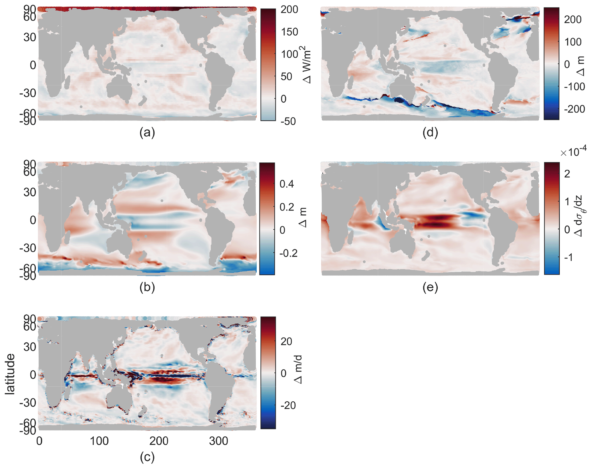
Figure 1Climate perturbation. (a) Change in maximum incoming short-wave radiation. (b) Change in annual-mean sea surface height (SSH). (c) Change in annual-mean vertical velocity at 100 m. (d) Change in annual maximum mixed-layer depth (MLD). (e) Change in annual-mean stratification at 100 m, , using 155 and 55 m potential density. All maps use a cylindrical equal-area projection.
2.2 Idealized tracers
2.2.1 Model formulation
Our aim in developing a set of idealized tracers to represent new production and export is to have a minimal model which allows us to explicitly connect responses of these biological rates to the physical climate perturbation described above. This section describes the assumptions used to design the tracers and their mathematical form, followed by a sensitivity analysis in the 2000s climate and the choice of a limited set of parameters to analyze further. To explicitly represent the supply of inorganic nutrients from depth and new production requires one nutrient tracer (e.g., McGillicuddy Jr et al., 2003); a second tracer can represent the phytoplankton that is created and follow it to depth. We assume an equivalence between new and export production due to the need for mass balance in steady state; thus, the annual supply of nutrients from depth, used in new production, is expected to match the downward flux of plankton and detritus (Eppley and Peterson, 1979).
In designing the nutrient tracer, we make three simplifying assumptions. First, we assume that the deep nutrient pool has a fixed concentration, not dependent on explicit remineralization, which decouples the nutrient tracer from the export tracer. This assumption will create different vertical nutrient gradients than models with remineralization included. Second, we assume that new production depends on the availability of this nutrient and light alone and not on the water temperature or on the existing plankton population that may be sustained by recycling of nutrients; this omits processes thought to be important in bloom-type events (Behrenfeld and Boss, 2014) but again keeps the nutrient and export tracers decoupled. One may reframe this choice as subsuming an effectively constant total phytoplankton concentration into μ0, which leads to an overestimate of growth when and where total concentration would be low and an underestimate of growth when and where total concentration would be high in comparison to a production function including the phytoplankton concentration. Finally, we assume that the light available for new production in the mixed layer is the mean of the light levels within the mixed layer (as done in McGillicuddy Jr et al., 2003); below the mixed layer, productivity depends on the light at only the depth in question. This choice increases subsurface growth within the mixed layer and decreases near-surface growth, while allowing growth below the mixed-layer depth.
With these assumptions, the reactions of the nutrient, N, are governed by the following equation:
where μ0 is the maximum growth rate (mmol N/m3 d), Q is the nutrient limitation (nondimensional), L is the light limitation (nondimensional), kN is the half-saturation constant for the nutrient (mmol N/m3), α is the sensitivity for the light limitation (m2/W), and S is the restoring source at depth. Light, I (W/m2), decays exponentially from the surface value of the incoming short-wave radiation but is averaged over the mixed-layer depth (defined by maximum buoyancy frequency criterion, Large et al., 1997). Thus, light has a constant value in the mixed layer and an exponentially decaying value below, which does allow growth below the mixed-layer depth. For m, N is continually reset to a value of 20 mmol/m3; this is our fixed nutrient pool. While the observed deep nitrate values vary on the basin scale, from about 13 mmol/m3 in the Arctic to about 38 mmol/m3 in the South Pacific (Garcia et al., 2013), this fixed N value at depth decreases drift in the solutions as only the upper ocean's nutrients must spin up. The initial conditions for N, which are used at the start of both 10-year time slices, are a linear interpolation between 20 mmol/m3 at 1000 m and 1 mmol/m3 in the surface grid cell. There is no flux through the air–sea or sea–land interfaces. The physical transport and mixing are done by the same mechanics as existing passive tracers in CESM-POP, with a third-order upwind scheme for advection and diffusive mixing that is spatially variable due to parameterizations of mixed-layer, submesoscale, and mesoscale isopycnal processes (see Sect. 2.2 of Danabasoglu et al., 2020, for details).
In designing the second tracer, we aim to explicitly represent the export from the surface to the deep ocean. This export is a combination of plankton and detritus but should be the same total mass, on average, as the supply of nutrient upward. We do not differentiate between different types of sinking organic matter and refer to them as a whole as particles. We assume that there is a constant sinking rate relative to the surrounding water and a small loss rate, which represents both remineralization into the recycled nutrient pool and removal through higher trophic levels. Particles, P, have their reactions governed according to the following equation:
where σ is the decay rate of particles (1/d), and ws (m/d) is the vertical sinking rate of particles. There is no flux through the air–sea or sea–land interfaces. Again, advection and mixing are applied by the existing CESM-POP mechanics for passive tracers.
2.2.2 2000s sensitivity
Our idealized tracers have five parameters: μ0, kN, α, σ, and ws. In order to identify reasonable values, we perform a sensitivity analysis of the first three under the early-century climate. The decay rate and sinking rate of P are held fixed at ws=0 m/d and d in this analysis, as they do not affect N or the production rate and only modestly affect the horizontal spatial patterns of P: faster decay reduces global-mean P, while faster sinking moves P deeper in the water column, with neither changing the basin-scale or latitudinal structure of annual-mean surface P. The values of the parameters used are a factor of 4 increase and decrease from μ0=0.5 mmol N/m3 d, kN=1 mmol N/m3, and α=0.05 m2/W, giving three values for each. We ran 10-year simulations under 2000 conditions for each of the 27 cases created by combining the options and examined the zonal and annual-mean fields the final year; while this system is not in complete equilibrium after only 10 years, most drift occurs in years 1–2. We do not see substantial differences in our climate change results when using year 5 or year 10 of the time slices in our computations.
To examine sensitivity to parameters and choose reasonable cases for the climate change experiments, N is compared to near-surface World Ocean Atlas nitrate distributions (WOA NO3, Garcia et al., 2013). P is compared to output from the CESM biogeochemistry model, BEC (Moore et al., 2013), which is run with the same model physics. Specifically, we compare near-surface P to total plankton, the sum of its three phytoplankton classes in carbon units, converted to nitrogen units using a stoichiometric ratio of 16 mmol N/117 mmol C. Although our particles represent both living matter and detritus, near the surface this P is most like newly produced plankton, which we expect to have the same spatial patterns as total phytoplankton. We choose this comparison to take advantage of the work done to fit BEC to observations for the same physics (see Fig. 4 of Moore et al., 2013) and due to the sparseness of phytoplankton concentration observations (e.g., Chl a data used in Boyce et al., 2010).
Overall, integrations with varied parameters for N mainly change its global-mean surface concentration and not the meridional structure (see Fig. 2a). This meridional structure matches that of surface global nitrate values qualitatively: high values in the subpolar regions, moderate near the Equator, and low in the subtropics. However, the Northern Hemisphere peak is shifted north, and the Southern Ocean values are low compared to observations, with the latter due mainly to our choice of a constant deep N concentration below that typical in the Southern Ocean. We will not be analyzing the Southern Ocean in detail, as we have not included iron limitation in our model, and this would be critical for the dynamics of production there. The annual and zonal mean nitrate from the BEC model are shown for reference (dashed line in Fig. 2a); this more detailed model also misses the location of the Northern Hemisphere peak, suggesting this may be due to the model circulation, but is much closer to observations in the Southern Ocean. Correlations between annual and zonal mean N and WOA NO3 are between 0.81 and 0.88 for the full active depth of 1 km and between 0.65 and 0.93 for just the surface. Changes in parameters affect the mean surface concentration of N in a predictable way: increasing kN increases the mean surface concentration, while increasing μ0 and α decrease it. Changing μ0 causes the largest change in magnitude and kN the least.
This relationship between parameters and near-surface N is the result of a balance between physical supply of N from depth and its consumption by production at a rate set by the parameters. If production is slower than supply, N will accumulate, increasing the production rate and decreasing the vertical N gradient and therefore the supply rate until a near equilibrium is reached. Thus, we can predict this relationship between parameter choice and near-surface N using the production function, μ0Q(N)L(I). The total production's dependence on N and I can be understood through the initial slopes of the production–nutrient and production–light curves, which are and μ0α: these describe how quickly production increases for an initial injection of each limitation; steeper initial slopes and faster initial production mean less accumulation of N before equilibration. Thus nutrient concentration will be higher for higher and ; these functions describe a two-dimensional space where increases along either axis decrease productivity and increase near-surface nutrient concentration.
We define a biological timescale as a single term to summarize these two axes. First, we recognize that has units of days, so we normalize α, which has units W/m2, by dividing by
to reach the same units as , m3/mmol N, so that also has units of days. We then add the results. The choice of this normalization factor is specific to this model, where we are forming an equivalence between a nitrate-type nutrient and light. Our α0 is an expression of how we stretch the light coordinate so that the initial slope of production with respect to I is in the same units as the initial slope of production with respect to N, suggesting α0 as a ratio of . Given the relative values of I and N, α0≤1 mmol N/W m is likely to be the most fruitful.
Now we see that we have a biological timescale for new production based on the parameters chosen; we call this biological timescale τbio:
The format of this timescale reinforces the qualitative relationship between surface N and changes in μ0, α, and kN. We can use τbio as a metric of how quickly production might consume a new supply of nutrients; if we compared it to a physical timescale for nutrient supply rate, τp, places where τbio is shorter are likely to be nutrient-depleted and places where τp is shorter are likely to be nutrient-replete. Across our 27 parameter cases, τbio ranges from about 2 d to 2 years. In Fig. 2b, τbio is compared to global-mean surface N for the 27 cases and correlates well, r=0.96. This correlation is best for this and similar values of α0, e.g., 0.1 or 2 mmol N/W m, but is lower for, e.g., 0.01 or 100 mmol N/W m. This is consistent with our understanding of α0 as a ratio of .
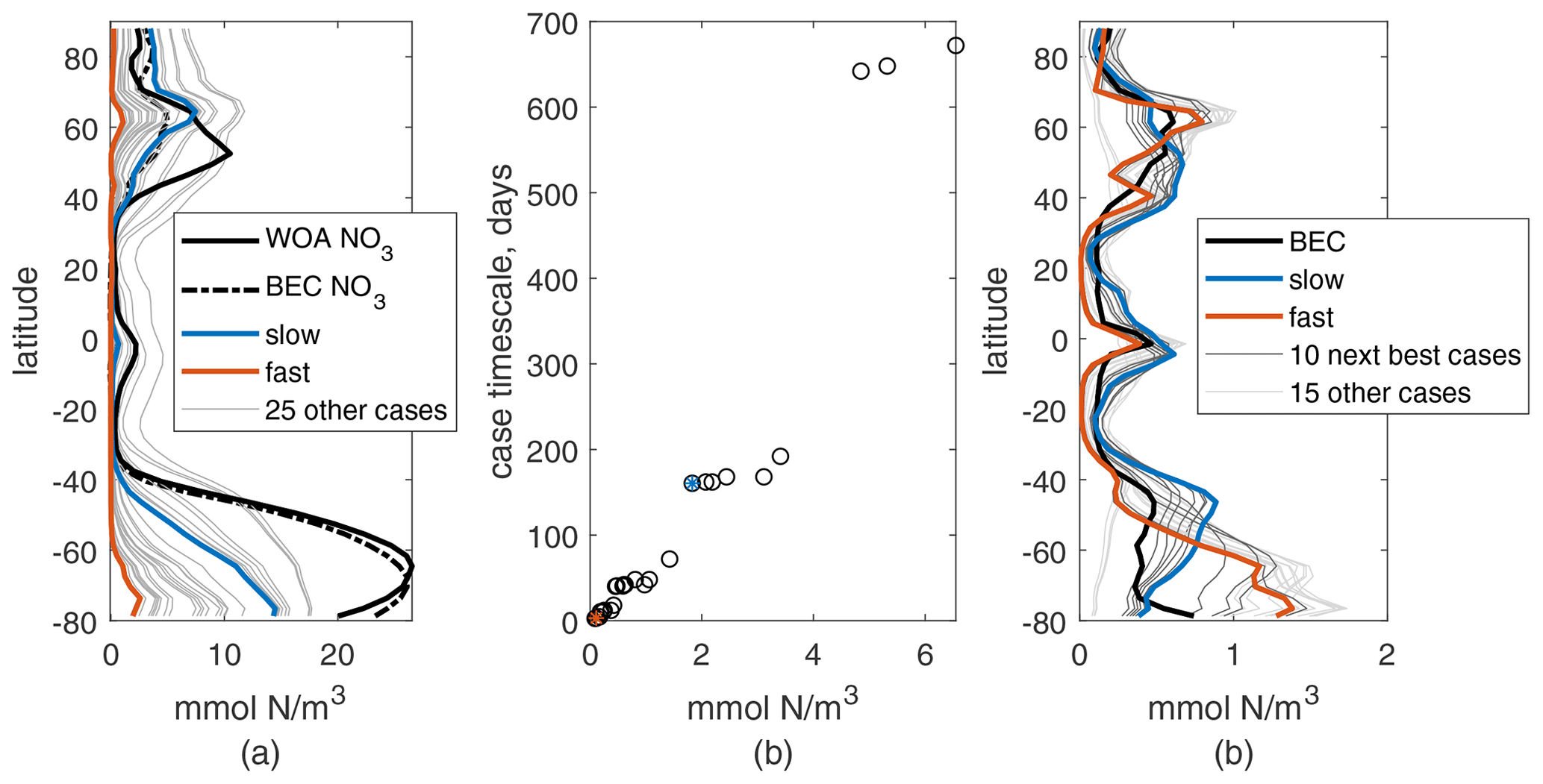
Figure 2Annual and zonal mean of surface N (a) and P (c) for 27 parameter choice cases from the 10th year of simulation. Values for the two chosen cases are shown in blue and orange. Annual and zonal mean references are shown by the thick black lines: nitrate from the World Ocean Atlas observations and from the BEC model in the same physics (dashed); total plankton mass from the BEC model. (b) Case timescale values vs. global annual-mean N (black circles); the two chosen cases are marked with blue and orange stars.
Meridional structures of P for these same integrations show more variation than N, which is clear in the more frequent intersections of the surface value curves and the variation in the latitudes of the maxima (Fig. 2c). The structure of the surface BEC phytoplankton has peaks near 60∘ N, the Equator, 45∘ S, and along the Antarctic coast. The three cases with lack these peaks entirely, with a much smoother structure that we consider a poor match for observed behavior and will not be considered further. To determine the best of the remaining options, we measured the correlation coefficient between the annual meridional structure of P and BEC phytoplankton, which ranged between 0.18 and 0.68 at the surface. The top half of these cases, 12 of the remaining 24 (see Table 1), were examined by eye for a good qualitative match at the surface and will be used for further analysis. These cases have the correct general latitudinal structure of P and also have reasonable new (export) production rates between 5.5 and 7.6 PgC/yr (Fig. 3a), which is within the 5–11 PgC/yr rate in most literature (e.g., Cabré et al., 2015).
We will not be examining the explicit sinking of our particles. For those interested, consider sinking rates, ws, consistent with estimates for detritus: single cells sink at about 0.1 m/d, and aggregates can reach over 100 m/d (Jackson and Burd, 1998). For decay rates, we suggest fixing these after choosing ws and adjusting them to have most production sink below the depth threshold of choice. For instance, with ws of 5 m/d, σ=1/yr has 95 % of the annual production sink below 100 m.
We choose two cases for detailed analysis which have P structures capturing different aspects of the BEC surface phytoplankton concentrations and quite different parameter and mean surface N values. The first case has surface P maxima near 45∘ N and S and the Equator, nicely matching those at the Equator and 45∘ S in BEC but missing the 60∘ N and Antarctic-coast peaks. This case has a small maximum growth rate (μ=0.125 mmol N/m3 d), a moderate light sensitivity (α=0.05 m2/W), and a low nutrient threshold for growth (kN=0.25 mmol N/m3). We consider this analogous to a small phytoplankton type or a phytoplankton community that has adapted to oligotrophic conditions, with plenty of light but low available nutrients. This case has a τbio of 162 d, corresponding to moderate mean surface N, slightly lower than WOA nitrate at the surface (see Appendix A for more details). We call this the “slow” case.
The second case has surface P maxima near 60∘ N, the Equator, and the Antarctic coast, similar to those at 60∘ N and the Equator in BEC and capturing the increase toward the Antarctic coast but missing the 45∘ S maximum. In contrast to the first, this case has a fast maximum growth rate (μ0=2 mmol N/m3 d), a low light sensitivity (α=0.2 m2/W), and a moderate nutrient threshold for growth (kN=1 mmol N/m3). We consider this analogous to a large phytoplankton type or a phytoplankton community that has adapted to higher-latitude conditions, with large seasonal cycles of light and nutrient availability. This case has a τbio of 3 d, corresponding to a very low mean surface N, which is noticeably below observed nitrate concentrations. We choose this case for large contrast with the first and call it the “fast” case. In the results section, we will focus on the changes in production under global warming for these two parameter cases of our idealized biogeochemical model and use the larger set of 12 cases for context.
Table 1Set of parameter values for 12 cases that compare best to WOA nitrate and CESM total phytoplankton. Each column represents three cases with . The range of τbio covers those for all three kN.

2.3 Light and nutrient controls on production
Under global warming, changes in light and nutrient availability will vary both spatially and temporally. This section describes our method to untangle the effects of these two components on changes in new production. The form of production, R=μ0QL, allows for a decomposition and attribution of changes in productivity to changes in nutrients and/or light. As μ0, the maximum growth rate, does not vary in space or time, we can examine simply the nutrient availability, Q, and the light availability, L, both of which are nondimensional and have values between 0 and 1, as does their product. Using model output of the monthly-mean N and R, we compute the monthly-mean for each grid cell and the monthly-mean . The reason for computing L in this way is that the mixed-layer depth, and thus L, can change rapidly. The production rate, R, and nutrient, N, are averaged online in our model, and thus computing L from them allows us to have a time-averaged L that would not be possible to compute from the time-averaged mixed-layer depth and incoming radiation. The change in QL can be decomposed as
where Δ indicates the change between the warmer, perturbed climate (2100) monthly values and those in the 2000s climate, as written out using subscripts of 2100 and 2000, and all terms can be averaged in space or time as needed. These difference terms are also nondimensional and have values between −1 and 1. Due to the way we compute L from R and Q, there is no residual term – the above equation holds to numerical precision. We will use this decomposition to analyze both the spatial patterns of annual-mean production and seasonal cycles of production. When one of the three right-hand terms is most similar in size to ΔQL and highly correlated in space or time, we will consider that term the main driver of changes in production.
For spatial correlations, or pattern correlations, we assume a decorrelation length scale of 10 grid cells, which is 6–9∘ latitude or longitude, depending on location. From examining the autocorrelation of several terms in Eq. (7), we find that this is a slight overestimate of the decorrelation length scale in some cases. The degrees of freedom in a pattern correlation over the global ocean are then 825, and pattern correlation coefficients larger than r=0.09 are significant.

Figure 3(a) Global annual new production integrated over the top 100 m for 12 cases for 2000 (black circles) and 2100 (red diamonds) vs. τbio (nonlinear axis for readability). (b) Percent change from panel (a), black stars; fast and slow cases circled in orange and blue, respectively. (c) Global mean N in the top 100 m vs. τbio. (d) Absolute change from panel (c).
3.1 Global statistics and dominant spatial patterns
For our 12 cases, global annual new production in the top 100 m is 5.3–7.5 PgC in the early-century scenario and decreases to 4.8–6.2 PgC in the late-century scenario; production is higher for shorter τbio in both epochs (Fig. 3a, b). These patterns hold for our two exemplar cases, with the slow case having lower new production and a smaller decrease than the fast case. Our 12-case range of decreases in production, 9.5 %–19.5 %, is similar to the 7 %–18 % range of export decreases in CMIP5 (Fu et al., 2016) but larger decreases than most net primary production changes in CMIP5, −2 % to −16 % (Fu et al., 2016), or CMIP6, +6 % to −12 % (Kwiatkowski et al., 2020). A large portion of this variability in global new production is related to the Southern Ocean, which is the basin with largest production and which our model does not represent well. Without the Southern Ocean the reductions in global annual production are 8.5 %–11 % – a range which is smaller than the range of export decreases in CMIP5 and within the range of net primary production changes in both CMIP5 and CMIP6.
Decreases in new production are partially determined by decreases in near-surface nutrient concentration. In all 12 cases, global-mean N concentration in the top 100 m decreases by 15 %–22 % in the late-century conditions (Fig. 3c, d). Both initial concentrations and absolute reductions are smaller for shorter τbio, but the small range of reduction percentages (15 %–22 %) highlight that the changes are somewhat insensitive to the varied light- and nutrient-limitation choices. These absolute reductions are 0.04–0.66 – a range which is slightly smaller than the reductions of 0.66±0.49 for CMIP5 RCP8.5 and 1.06±0.45 for CMIP6 SSP5-8.5 (Kwiatkowski et al., 2020). Despite the small absolute reductions in near-surface N concentration, the decrease in global new production is larger for fast cases with the shorter case timescale (Fig. 3b); these shorter τbio cases have lower near-surface nutrient concentrations in the early-century conditions and higher slopes in their production–nutrient curve, making them more sensitive to changes.
The spatial patterns of annual production under early-21st-century conditions demonstrate one effect of τbio (Fig. 4a–b). The slow case has lower maximal values, as expected given its lower maximal growth rate, and smoother variations in space. The fast case has higher maximal values of new production, again set by its maximal growth rate, and sharper variations in space, due to its greater need for nutrients in order to grow: production is more limited to locations with a fast physical nutrient supply. Despite these differences, both cases match the general meridional patterns of observed phytoplankton (see, e.g., Dasgupta et al., 2009 for observations), with higher values in the subpolar and equatorial regions and lower values in tropical–subtropical regions.
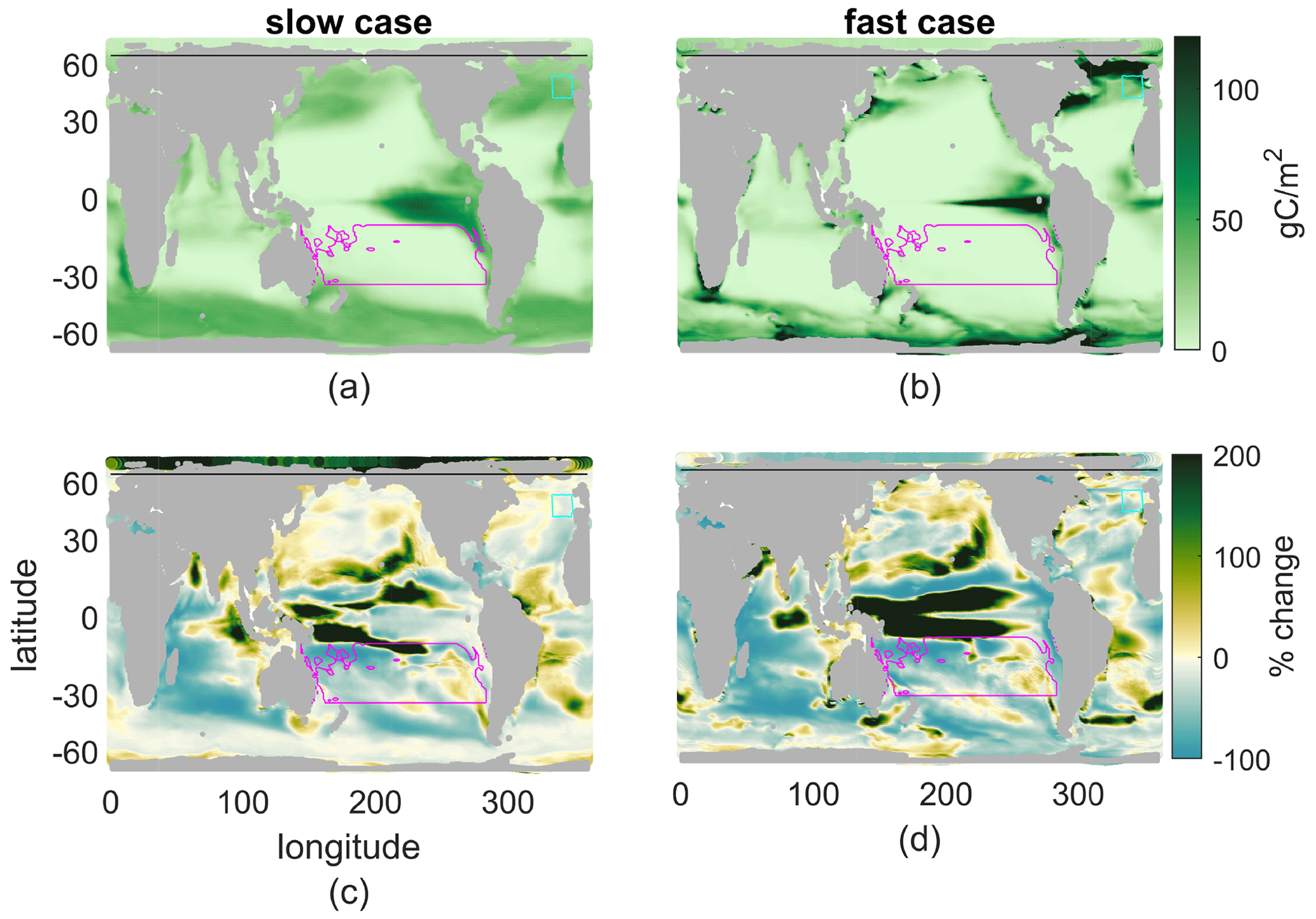
Figure 4(a, b) 2000s annual production integrated over the top 100 m. (c, d) Percent change with climate perturbation. (a, c) Slow case. (b, d) Fast case. The magenta contour indicates the subtropical South Pacific, cyan the Porcupine Abyssal Plain, and the black line the southern edge of the Arctic.
The spatial patterns of change in production under the warmer climate are qualitatively similar for both cases, with broad moderate reductions over most of the oceans, including the Indian Ocean, the South Pacific, and the North Atlantic (Fig. 4c–d; the pattern correlation is r=0.26; see Table 2 for all pattern correlations). Both cases also contain common areas with increased production in the 2100s, including most notably the edges of the equatorial Pacific, where upwelling has spread latitudinally, and the southern edge of the subtropical North Pacific Gyre. Despite broad similarity in the productivity response between the fast and slow cases, there are many small regions where the sign of the climate change response differs, perhaps most notably the Arctic, the central equatorial Pacific, and the Bay of Bengal. These are regions with qualitative as well as quantitative sensitivity of the climate perturbation reaction to the light and nutrient functions of uptake.
While we do not discuss spatial patterns in detail for the larger set of parameter cases, we do compute production by basin (Appendix, Fig. B1). For every basin but the Arctic, production decreases for a warmer climate in all 12 cases, indicating that the qualitative results in most basins are not sensitive to the specifics of light and nutrient limitations. In the Arctic, which has the least total production, the four cases with lowest τbio have decreases in new production, while the remaining eight have increases. We will discuss this sensitive region further in Sect. 3.5.
As global reductions in production were matched by reduced nutrient concentrations, so too can spatial patterns in production be linked to nutrient concentrations and the vertical nutrient flux. Although the nutrient flux and new production do not necessarily align in space and time, we empirically find pattern correlations between the annual-mean production and the nutrient flux at 100 m as well as the mean nutrient in the top 100 m (Fig. 5). The vertical flux is somewhat more noisy; hence the correlations of the absolute changes between present and future are only r=0.51 and r=0.14 for the fast and slow cases, respectively (see Table 2 for all pattern correlations). The mean nutrient concentration in the top 100 m reflects the integrated effects of the flux, the stronger vertical mixing in the mixed layer, and productivity; hence the correlations are somewhat stronger. We note that the variations in nutrient concentrations within the mixed layer are typically small – less than half the mean concentration and much less than kN; these variations lead to slightly lower production rates than those that would occur if the nutrient concentrations were constant from the surface to the mixed-layer depth. In the present day, the pattern correlations between annual nutrient concentration in the top 100 m and production integrated to 100 m are r=0.56 and r=0.26 for the fast and slow biogeochemistry; for the future they are r=0.58 and r=0.33, and for the percent changes they are r=0.88 and r=0.48, respectively. Across our 12 cases, the lower τbio cases, which are more nutrient limited, have stronger correlations between nutrient concentration in the top 100 m and productivity. These correlations are always stronger in the warmer climate, when all cases are more nutrient limited.
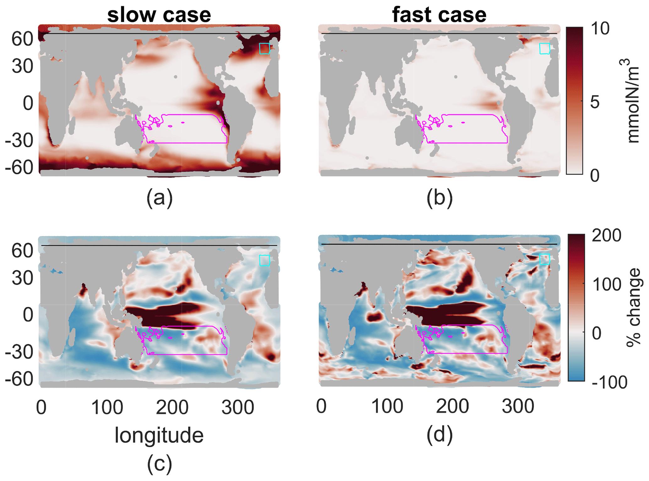
Figure 5(a, b) Nutrient concentration, mmol N/m3, averaged over a year and the top 100 m. (c, d) Percent change of this field from 2000s to 2100s climate. (a, c) Slow case. (b, d) Fast case.
While we have connected the production and its changes to nutrient concentrations, light effects are also important. Productivity is a product of functions representing the sensitivity of productivity to light L(I) and to nutrient Q(N) availability. As described in the methods, this allows a decomposition of the changes in production into those caused by changes in nutrient availability, LΔQ; those caused by changes in light availability, QΔL; and the covariance of the two, ΔQΔL. Examining the spatial patterns of QL, its change (Δ(QL)), and the components of that change (Fig. 6) provides more details on the controls of reduced production beyond the vertical nutrient supply and surface concentration. From the spatial fields of these terms, all annual means averaged over the top 100 m, QL, and Δ(QL) show the same spatial patterns as production and its changes, respectively, as expected by definition. However, Δ(QL) looks somewhat different from the percent changes in production shown before (Fig. 4). From the components of the change, it is clear that LΔQ is the main control on production: r=0.74 and r=0.64 for the fast and slow cases, which is consistent with our discussion of nutrient supply and concentration (Fig. 6b, c, g, h). The change in light availability is a smaller contributor: r=0.19 and r=0.43 for the fast and slow cases (Fig. 6d, i). Finally, the covariance is anticorrelated to the total change: and for the fast and slow cases (Fig. 6e, j); these correlation coefficients are insignificant. This component is largest near the Equator, where it offsets increases in nutrients due to broader upwelling in the warmer climate. These pattern correlations are qualitatively similar without the Southern Ocean, which we do not represent well with this model.
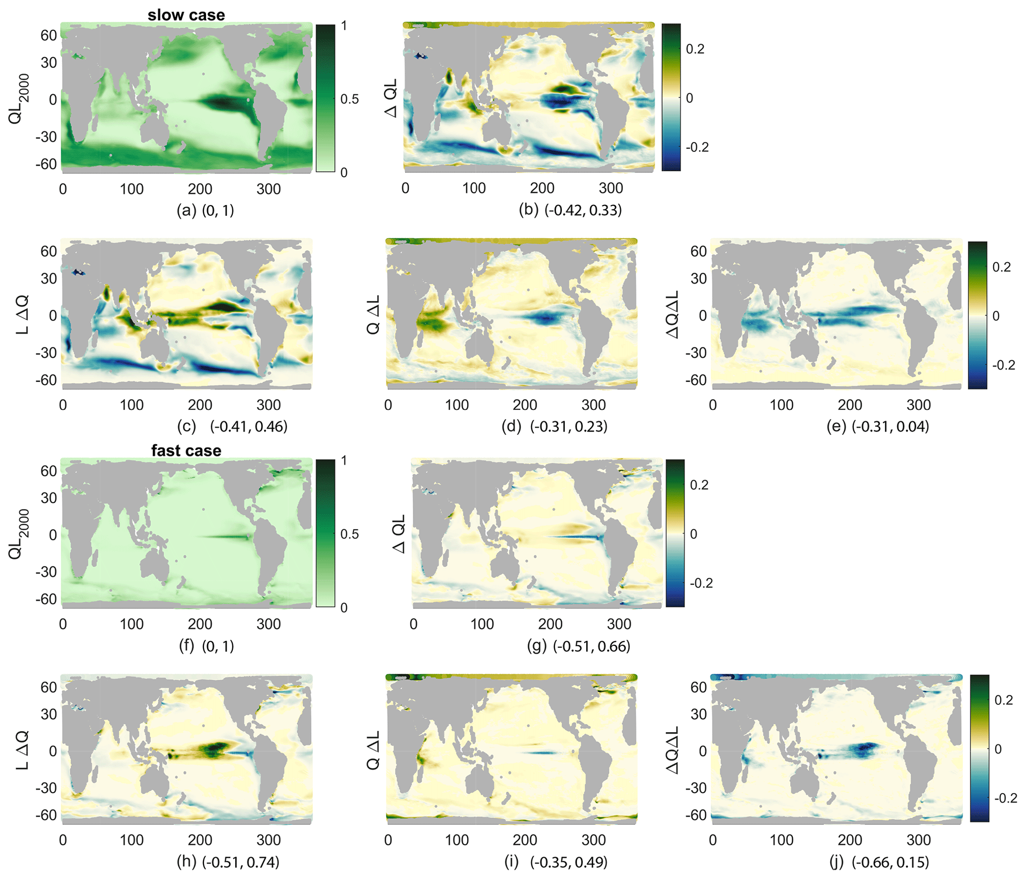
Figure 6QL for 2000s climate (a, f), its change (b, g), and its components, all averaged over 1 year and the top 100 m and then normalized by the maximum of QL (nondimensional) in the 2000s. (c, h) LΔQ, (d, i) QΔL, and (e, j) ΔQΔL. (a–e) Slow case, normalized by 0.055. (f–j) Fast case, normalized by 0.14. Minima and maxima for each plot are given following the panel letter.
From these analyses, we see that qualitatively the spatial patterns of the response to the climate perturbation are similar across the biogeochemical cases under consideration, likely pointing to strong controls by the underlying physics via the nutrient supply. Quantitative differences exist; the spatial differences point to locations where results are sensitive to model parameters, while the global differences are consistent with the chosen parameters in that the faster cases, which have higher production and lower near-surface nutrients, have new production more correlated with the reductions of near-surface nutrients and their vertical supply.
Table 2Pattern correlations for annual-mean fields. Bold values indicate significance. All production, production component, and nutrient concentration (N) fields are the mean over the top 100 m, and all fluxes are at 100 m depth.
3.2 Global seasonal cycle
Over much of the ocean, the seasonal cycle is the dominant mode of productivity variability due to seasonal variations in light and nutrients. We are interested in how the seasonal cycle will respond to our climate perturbation and whether this is sensitive to the case parameters.
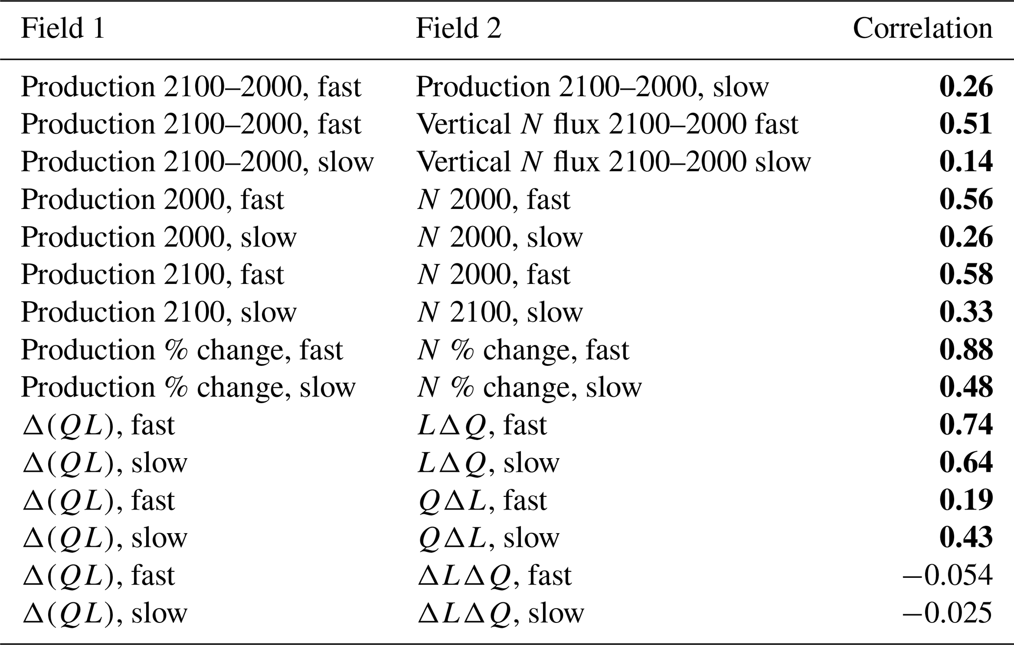
We define the global seasonal cycle as monthly global spatial averages with a 6-month offset between the Northern Hemisphere and Southern Hemisphere so that the boreal and austral seasonal cycles are in phase. Differences in the seasonal cycle of new production between the fast and slow cases are large and are a reflection of the different τbio of the cases (Fig. 7b). Seasonal changes in nutrient and light availability have physical timescales of weeks to months, which are between the τbio of 3 d for the fast case and 162 d for the slow case. Both cases have high upward nutrient flux in the winter and early spring (Fig. 7a) in conjunction with deep and dense winter mixed layers. However, the strong nutrient flux occurs over a shorter period of time in the slow case as the physical supply overwhelms the slow ecosystem's ability to consume and thereby reduces the flux. Productivity in the fast case quickly consumes the nutrients as they are supplied in the late winter and spring, whereas productivity in the slow case spreads out the nutrient consumption, achieving its maximum in midsummer when the light is most plentiful (Fig. 7b).
Despite the qualitative differences between the present-day seasonal cycles, climate change has a qualitatively similar impact on both the fast and slow cases (Fig. 7a–c). The peak wintertime nutrient flux at 100 m (Fig. 7a) is reduced by 22 % and 21 % in the fast and slow cases, respectively. This reduction is consistent with, but may not be entirely caused by, reduced winter mixed-layer depths restricting the entrainment of nutrient-rich water from the thermocline (Fig. 7f). Production is reduced during all months but particularly in the latter half of the respective growing seasons. Thus, the growing seasons during the 2100s are modestly shorter with earlier peaks in both cases. It is true across all 12 cases that the largest reductions in new production are after the peak new production. Thus, we can conclude that while the seasonal cycle can be very different across cases, for this model the global reduced production in a warmer climate follows a consistent pattern of a shortened growing season.
The causes of reduced production can be identified through the seasonal cycles of the components of ΔQL, all of which are small fractions of the maximum early-century QL values. In both slow and fast cases, winter and spring increases in light availability due to shallower MLD are offset by reductions in the nutrient availability and light–nutrient covariance, leading to reduced production (Fig. 7d, e). The minima of ΔQL are in the second half of the growing season in both cases, driving the shortened season. The slow case has negative values of all components at this time, with nutrient availability being the most negative (Fig. 7d). By contrast, the fast case's minimum of ΔQL occurs while QΔL is positive and reduced production is driven by both reduced nutrient availability and the light–nutrient covariance (Fig. 7e). This large ΔQΔL in the fast case during the growing season is obscured in the annual mean (Fig. 6), where this factor is small over most of the ocean and insignificantly correlated to the total change. In both our cases, reduced nutrient availability is a major contributor to the shortened growing season, indicating a consistent mechanism for reduced total production in response to the climate perturbation.
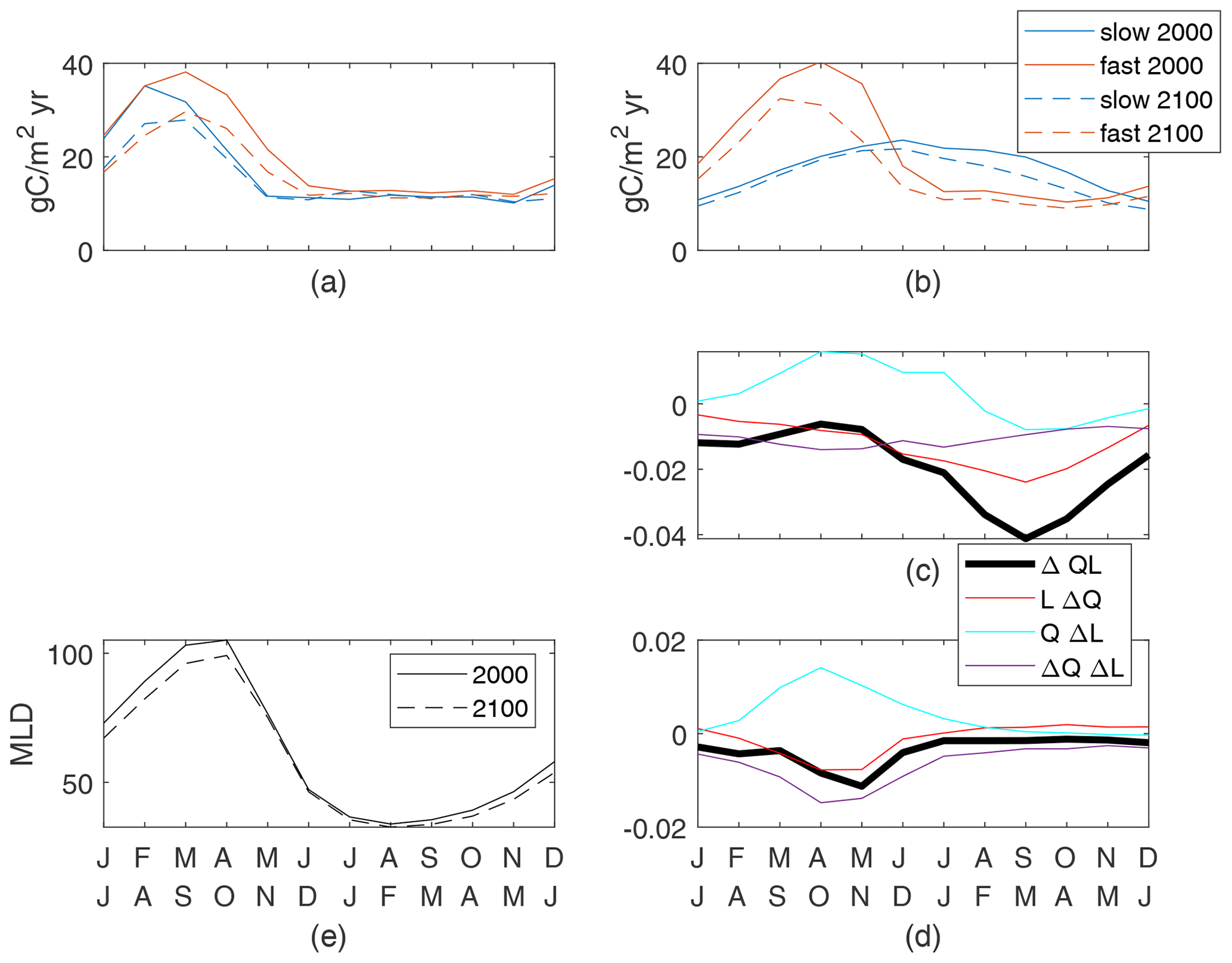
Figure 7Globally integrated supply of nutrients (a) and production of particulates (b) for the top 100 m. Both cases are shown for the 2000s and 2100s; the seasonal cycle is the mean of simulation years 8–10. Production controls (nondimensional) for the slow case (c) normalized by a global maxQL(2000) value of 0.055 and the fast case (d) normalized by a global maxQL(2000) value of 0.14. (e) Mean mixed-layer depths.
3.3 Regional case studies
We next examine three regions in detail: the downwelling South Pacific, the Arctic, and the Porcupine Abyssal Plain in the North Atlantic. These three regions exemplify the spatially varied processes driving the climate response and the sensitivity of that climate response across our model cases (Figs. 4, 6). We emphasize that none of the model cases closely match observations in any particular region (see Appendix A for a comparison of N and observed nitrate) and that these examples are chosen for their qualitative differences. To contextualize these regions, we note their physical biomes; biome analysis has been used previously to identify ocean regions with similar biogeochemically relevant physical characteristics across basins (Sarmiento et al., 2004; Cabré et al., 2015). A further discussion of biome analysis across the broader 12 parameter cases is available in Appendix B.
The downwelling South Pacific (red outline in Fig. 4), part of the permanently stratified subtropical biome, is a region with small seasonal cycles, small climate-induced changes in physics, and broad losses in production across model cases. These losses of production are driven by the same processes in the fast and slow cases, suggesting an insensitivity to parameter choices. By contrast, the Arctic (north of 66.5∘ N, the black line in Fig. 4), in the ice and marginal ice biomes, has large climate-induced physical changes, mainly in ice coverage. As noted earlier, the climate response in the Arctic is sensitive to parameter choice; this region is the most sensitive of those we discuss, with changes in annual new production having opposite signs in our two cases. The Porcupine Abyssal Plain (blue outline in Fig. 4), in the seasonally stratified subtropical biome, has deep winter mixing in the present climate and large decreases in mixed-layer depths with the climate perturbation. This region is an example where the main driver (light or nutrients) of the climate-change-induced reductions to productivity changes across parameter space. These three regions provide illustrative examples demonstrating how physical climate changes create a range of possible responses in new production, as mediated by the parameters that modify the sensitivity of productivity to light and nutrient availability, and thus how the sensitivity of projected changes in new production varies across the world oceans.
3.4 South Pacific
The downwelling South Pacific is defined by annual-mean downward vertical velocity at 100 m depth in the South Pacific between 10 and 35∘ S. Maximum winter mixed-layer depths reach only 120 m, putting this region mainly in the permanently stratified subtropical biome. Here, all biogeochemical parameter cases are qualitatively similar in both their current-climate seasonal behavior and their response to the climate perturbation, which we show is driven by reduced vertical nutrient supply.
The seasonal cycles in this region in both early- and late-century climates have high values of both upward nutrient flux and new production in the austral winter and spring (Fig. 8a, b). Peak upward nutrient flux is in August in both cases in the early- and late-century conditions. In the fast case, peak new production is in the same month, indicating a fast response to the supply of nutrients. In the slow case, there is a 1-month delay, indicating a slower response. These peak times do not change between early- and late-century conditions; only the overall magnitude of rates decreases: in the slow case, annual production decreases by 25 % from 0.11 to 0.086 PgC/yr, while in the fast case, annual production decreases by 39 % from 0.045 to 0.027 PgC/yr. This is consistent with the global production being more reduced in the fast case than in the slow case. This pattern holds across the 12 cases, with all having peak production in August through October, no change in the peak timing with climate, and larger decreases in production for shorter τbio.
The decrease in new production is due to the reduced availability of nutrients. The total change in production, Δ(QL), is nearly identical to the changes due to nutrient availability, LΔQ, with rms differences of and for the fast and slow cases (Fig. 8c); this near match holds across all 12 parameter cases. This is consistent with Cabré et al. (2015), who saw decreases in production in low-latitude nutrient-limited biomes across models. Our addition to that analysis is the direct quantitative connection to reduced nutrient availability that is not straightforward to compute for more complex biogeochemical models.
The reduced nutrient availability is due to reduced upward fluxes of nutrients, which we can exactly identify (Fig. 9a, b). These fluxes are comprised of downward advective fluxes, upward fluxes from parameterized vertical mixing (Large et al., 1997), and upward fluxes from vertical effects of parameterized along-isopycnal mixing (Redi, 1982; Gent et al., 1995). Both components of parameterized mixing show reduced annual fluxes in the warmer climate at 100 m. Neither mixed-layer depths nor effective vertical diffusivities change substantially – less than 10 % for all MLD and less than 10 % across of the grid points in this region for diffusivity. Thus, reduced is the driver of the decreased upward nutrient flux.
The changes in spatial-mean nutrient profiles (Fig. 9c) show a consistent pattern across the fast and slow cases: increased nutrient at 350–650 m depth but decreases from 350 m to the surface, including decreases near 100 m. These mid-depth nutrient changes are due to physical changes in circulation and/or mixing in the main thermocline. For diffusive transport, the decreases in N concentration above 350 m mean that the vertical gradient of N near 100 m, where we measure the fluxes, decreases. Thus, the decreased production in the downwelling South Pacific is being driven by decreased nutrients below the deepest winter mixed layers (about 120 m), through decreased causing decreased diffusive fluxes, decreased near-surface nutrients, and thereby decreased nutrient availability, Q. From these two examples it seems likely that the causes of reduced nutrient availability in the warmer climate, which drives reduced production, are consistent across parameter cases.

Figure 8Subtropical South Pacific nutrient supply (a) and production of particles (b). Production controls (c) normalized by maxQL(2000) values in the region: 0.032 for the slow case and 0.013 for the fast case.
Figure 9(a–b) Annual-mean upward N flux components, gC/m2 yr, at 100 m depth, averaged over the subtropical South Pacific, for the 2000s and 2100s climate and their difference. Parameterized vertical mixing (“vert mix”), vertical component of parameterized isopycnal mixing (“iso mix”), and advection (“adv”) from model diagnostics. (a) Slow case. (b) Fast case. (c) Profiles of change (2100–2000) in annual-mean subtropical South Pacific nutrients.
3.5 Arctic
The Arctic region is defined as being within the Arctic circle (north of 66.5 ∘N) or equivalently having at least 1 d per year with no incoming solar radiation. This region has the largest sensitivity of changes in new production to model light and nutrient limitation, with the range across 12 parameter cases being a decrease of 17 % up to an increase of 52 %. Here, our two example biogeochemistry cases have notably different responses to climate change, with the slow case having a 46 % increase in annual production and the fast case having a 16 % decrease.
Seasonal cycles in the 2000s are similar for the fast and slow cases. In this region, that is an upward flux of nutrients year-round and high new production rates in the summer, with a peak in May for the fast case and September for the slow case (Fig. 10a, b). Under late-century conditions, the peak production of the fast case is in the same month, with a slight increase in production earlier in the year and reductions later in the year which lead to a total decrease; in contrast, the peak production of the slow case is much higher and is earlier – now in July. These regional-mean production shifts are consistent with the different responses seen in the annual production maps (Fig. 4), where the slow case has large increases while the fast case has moderate changes of both signs.
In the Arctic, increases in incoming light, with the seasonal maximum of the regional mean more than doubling (91 to 202 W/m2), are due to reduced sea ice (Fig. 1a) and have a large impact on changes in production. The mean increase in light availability in summer, quantified by QΔL, its effect on changes in production, is nearly as large as the maximum QL in the 2000s for both cases (Fig. 10c, d). In the slow case, this increase in light allows for a large increase in production in the first half of the growing season, until nutrients are slightly depleted by that production, reducing production through lower nutrient availability in the second half (negative LΔQ and ΔQΔL). This pattern is qualitatively consistent across slow cases with long τbio. In contrast, the increase in light availability in the fast case is offset by an associated reduction in nutrient availability, such that . Increased light in the spring leads to immediate increases in production (April), which uses enough nutrients to cause a dip in nutrient availability (May) before peak light availability (July), leading to decreased production in the summer and fall. This pattern is consistent across the four cases with shortest τbio, which have decreased annual production in the warmer climate (Fig. B1). Thus, in the Arctic, the increases in light availability consistently increase production in spring, leading at some point to a biologically driven decrease in near-surface nutrients. The resultant changes in production may take either sign and depend on the speed at which nutrients are removed, consistent with our τbio.
The Arctic is a region where changes in new production under global warming is highly sensitive to the formulation of model production, both for our model and more complex ones. Vancoppenolle et al. (2013) found that CMIP5 projections of Arctic NPP were dependent on whether the Arctic reached a nutrient-limited state post-sea-ice loss, with those models that reach a nutrient-limited state having reduced production and others having increased production in the warmer climate. Our analysis provides a mechanistic hypothesis for these differences: shorter τbio models have lower near-surface nutrients in early-century conditions, and therefore increases in production with increased light will more quickly lead to a nutrient-limited state.
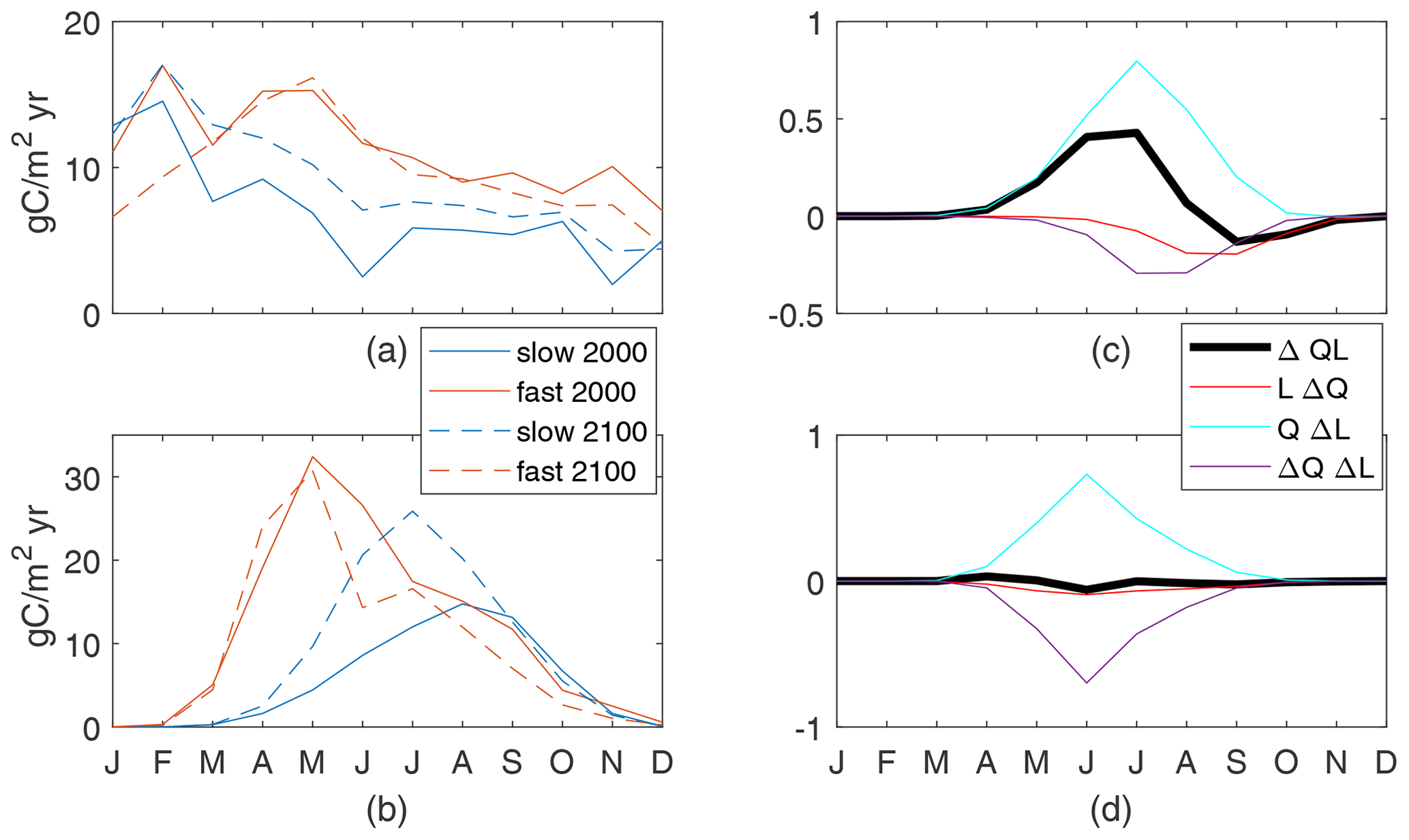
Figure 10Arctic nutrient supply (a) and production (b). Production controls on the slow (c) and fast (d) cases, normalized by the maximum values of arctic maxQL(2000): 0.021 for the slow case and 0.028 for the fast case.
3.6 North Atlantic
The Porcupine Abyssal Plain in the northeast North Atlantic is defined here to be 40–52∘ N and 27–11∘ W (cyan box in Fig. 4); this includes the location of the Porcupine Abyssal Plain Sustained Observatory. This region is characterized by deep winter mixed layers and net downwelling. Under a warmer climate, the winter mixed-layer depths are reduced; the spatial mean of the maximum decreases from 280 to 229 m, and the absolute maximum MLD is reduced from 669 to 590 m (Fig. 11d). All 12 cases have decreased new production in the future, 9.55 % to 26.75 %, which is a smaller range than our other two regions but still larger than the global ocean; our two example cases have a decrease of 12 % for the slow case and 21 % for the fast case. In this region, as for the Arctic, the mechanisms driving the changes vary.
In this region, our two model cases show qualitatively different seasonal cycles with production mainly in the early spring for the fast case and spread over the summer for the slow case (Fig. 11b) similar to their respective global cycles. Both cases have little qualitative change between the early and late 21st century. Most of the nutrient supply is in the winter for both cases (Fig. 11a), mainly due to wintertime entrainment associated with the mixed layer.
In the warmer climate, changes in production, ΔQL, depend on the relative impacts of increased light availability, QΔL, in March and April and decreased nutrient availability, LΔQ, in all months; the signs of these drivers are consistent across cases, but the signs of the change in production are not. In the slow case, the changes in production with climate are an increase in spring and a decrease in summer and fall for a total decrease, closely following changes in light availability, Δ(QL)≈QΔL (Fig. 11c). The increased light in March and April corresponds to shallower mean and maximum mixed-layer depths, respectively. Light availability decreases in the summer, due to increased mixed-layer depths in May and June. In the summer and fall, a higher portion of the reduction in production is due to reduced nutrient availability from both the lower winter peak in nutrient supply and the increased use during the spring production.
In the fast case, the same physical changes of the climate perturbation result in production decreases due to reduced nutrient availability in all months, Δ(QL)≈LΔQ (Fig. 11c). The winter increase in light availability has no noticeable impact, with substantially lower winter–spring production co-occurring with the lower nutrient flux (Fig. 11a) and shallower monthly-mean mixed-layer depth (Fig. 11d). This region's changes in new production are sensitive to parameter choices. Although total new production is reduced in both cases, reduced winter mixed-layer depths can act to either increase or decrease spring production, depending on whether that production is more sensitive to light, as in the slower cases with longer τbio, or nutrient availability, as in the faster cases with shorter τbio. These differences highlight the usefulness of this idealized model, which allows us to diagnose these drivers.

Figure 11Porcupine Abyssal Plain nutrient supply (a) and production of particles (b). Production controls (c), normalized by maxQL(2000) values for the 2000s: 0.022 for the slow case and 0.015 for the fast case. The discrepancy for the slow case is mainly due to LΔQ. Range and mean of monthly-maximum MLD (d).
In order to study the sensitivity of the climate response of new production, we designed an idealized, two-tracer biogeochemical model that explicitly represents nutrient supply to the photic zone, new production, and the export of organic particles. The chosen simplifications for the production function allow for detailed analysis of the causes of changes in production but eliminate or exaggerate certain aspects. First, dynamic phytoplankton concentration is omitted from the model; productivity is generally thought to scale with this concentration, so our seasonal results may be inaccurate in regions with strong blooms. Second, the lack of nutrient remineralization contributions to the nutrient field and the constant value of the deep nutrient pool remove a mechanism of production feedback which can affect its climate sensitivity. Third, the formulation of light limitation, using an average light concentration within the surface mixed layer, does not allow self-shading and enhances production in the lower portions of the mixed layer. Finally, the simulations are not constrained to be realistic; the results provide information about the key parameter sensitivities.
From model integrations under early- and late-21st-century climate scenarios with 12 different parameter sets, we found that global production, near-surface nutrient concentrations, and projected changes in production were all connected to τbio, derived from the initial slopes of the production–nutrient and production–light curves, which are the partial derivatives of production with respect to nutrients and light at the origin. A short τbio indicates faster production and higher nutrient utilization, leading to lower near-surface nutrient concentrations and faster nutrient supply; these then indicate larger reductions in global production in a warmer climate. These reductions were linked to reduced near-surface nutrient availability and a shortening of the growing season in all cases. The percentage decreases in global new production were different by about a factor of 2 between the highest and lowest τbio, a range similar to CMIP5. However, we find that the sign of the response (a reduction in productivity with warming) is the same for all of the light- and nutrient-limitation parameters that we considered.
We examined two exemplar cases, focusing on the similarities and differences in the seasonal, spatial, and regional responses to climate change. Spatial patterns of changes in annual new production are similar between these two cases (pattern correlation r=0.26), with both being correlated to the changes in annual-mean nutrient availability (LΔQ), near-surface nutrient concentrations, and upward nutrient flux. Correlations were stronger for the fast case, which is more nutrient limited. The ability to quantify the component of the reduction due to nutrient availability is unique to simple models like ours.
For more details on the drivers of the climate response and its sensitivity, we examined three regions. The South Pacific region demonstrated the most consistent response to the climate perturbation. Here, changes in light and MLD are negligible. Decreased nutrients in the upper thermocline drive lower vertical supply, lower nutrient availability, and lower production in all months for both exemplar cases. While there are still larger decreases for shorter τbio, the mechanism is not sensitive to biogeochemical parameters.
From our detailed analysis of two higher-latitude regions, we found that compensation between changes in light and nutrient availability has very different impacts for our runs with different production parameters. In the Porcupine Abyssal Plain, a reduced depth of the winter mixed layer acts to either increase or decrease spring production, depending on whether that production is more sensitive to light, as in the longer τbio cases, or nutrient availability, as in the shorter τbio cases. In the Arctic, larger increases in light availability due to sea-ice losses drive the largest sensitivity of new production's response to the climate perturbation, with different cases having opposite-signed annual-mean responses. Here, for fast cases (short τbio) light-driven increased spring production reduces nutrient availability and thereby production later in the growing season to such an extent that annual totals are reduced. In contrast, slow cases can produce more throughout the growing season with little impact on nutrient availability. This analysis suggests a mechanism for the variation of projected Arctic production in CMIP5, where reduced production was associated with nutrient limitation (Vancoppenolle et al., 2013): if τbio were diagnosed for those models, it may be that short τbio cases have higher nutrient uptake, driving the nutrient limitation and reduced production.
Biological rates like τbio are useful for explaining CMIP results more broadly. In those more-complex models, the effective τbio may vary in space because of changes in the phytoplankton community composition. It would be possible to quantify τbio for these models empirically in a vertical column ocean through the individual injection of each nutrient at several concentrations to find the slope of the production–nutrient curve. Alternately, the new production rates from many locations in a global ocean configuration could be used to fit a production curve over all nutrients, with τbio formed from the derivatives. While computing an effective τbio is outside the scope of this work, we believe developing a reusable procedure for these intermediate-complexity models to be a useful next step toward interpreting climate change production projections. Variations between model results might then be related to their different τbio, along with a comparison to the different physical rates.
We suggest that this reduced-complexity model and time slice method may be suitable for high-resolution climate change process studies where computational cost is a limiting factor. Having only two tracers, this model is as inexpensive as possible while explicitly representing the supply of inorganic nutrients, new production, and sinking export. Given the range of production parameters that provide reasonable global results, one can choose the ones most suitable for the question of interest, such as approximately matching an ecosystem in a particular region or biome. While not considered in this work, the formulation of P allows for changes in export efficiencies under a warming climate to be studied through changing ws and σ.
In our work, we were aiming to understand the sensitivity of the climate response and thus a wide range of possible model behaviors. To that end, our validation or comparison to observations and another, fitted, model was quite simple. For further context on how our two exemplar cases do (not) match observed behaviors, we show here the seasonal cycle of the 100 m averaged N concentration compared to WOA nitrate concentrations. Figure A1 provides the mean of monthly 100 m averaged WOA nitrate concentrations globally and for each of the three regions further examined in the text, along with the monthly 100 m averaged mean N concentrations. In all cases, our fast model concentrations are quite low. For the slow case, values are often in the 90 % range of WOA concentrations (not shown) but below the mean. The exception is the Porcupine Abyssal Plain region, where the slow case has N similar to nitrate but with a shift in the seasonal cycle. If future process work were to concentrate on an individual region, an analysis like this would allow for fitting of parameters.
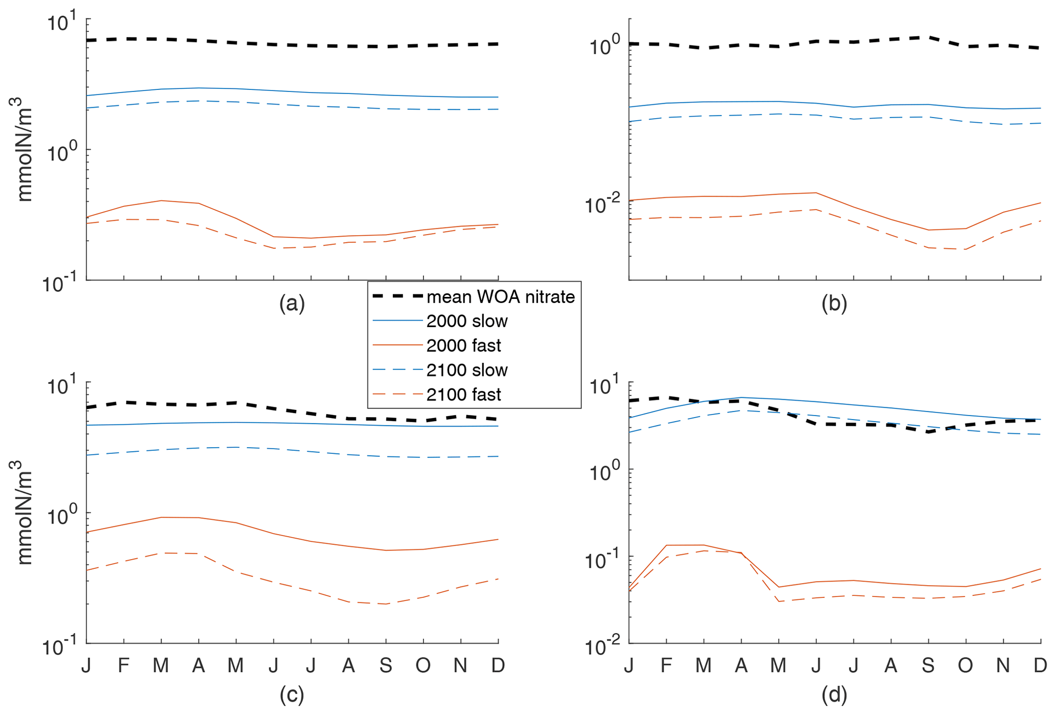
Figure A1Mean of monthly 100 m averaged WOA nitrate concentrations and the monthly 100 m averaged mean N concentrations for both fast and slow cases in 2000s and 2100s conditions. (a) Global ocean, with 6-month offset for the Southern Hemisphere, (b) subtropical South Pacific, (c) Arctic, and (d) Porcupine Abyssal Plain. Note that the y axis is a log scale.
This Appendix provides additional context of how our simple biogeochemical model's new production changes for different parameter values under the same physical climate perturbation. We provide a simple analysis of production changes across ocean basins and biomes for the 12 parameter cases lightly considered in the main text. The fast case in the main text is here labeled by case timescale 3, and the slow case is labeled by case timescale 162 (it is the rightmost 162 in figures). Global production rates and their changes in the warming climate were in Fig. 2.
First, we shown ocean basin averages of new production and its changes (Fig. B1). These basins should be self-explanatory, but note that the Southern Ocean begins at 35∘ S and the Arctic at 66.5∘ N. For all 12 cases, the Southern Ocean is most productive, likely related to our lack of iron limitation, and all basins except the Arctic show reduced new production in the warmer climate for all parameter cases. The largest percent losses are in the Southern Hemisphere basins, and parameter cases with shorter τbio show larger reductions than those with longer τbio.
Second, we show ocean biome averages of new production and its changes. Biome delineations are based on latitude, sea-ice fraction, annual-mean vertical velocity at 100 m, and maximum annual mixed-layer depth. In the ±5∘ latitude band we have upwelling and downwelling regions, noted Eq U and Eq D. Outside the equatorial band, downwelling regions are subtropical, ST, either seasonally stratified (maximum mixed-layer depths >150 m), ST SS, or permanently stratified (the opposite case), ST PS. Upwelling regions in 5–30∘ N, 5–35∘ S are the low-latitude upwelling biome (LLU); above that, they are subpolar (SP) unless their ice fraction goes above 0.1 some month. Ice biomes are split for the Northern Hemisphere and Southern Hemisphere, noted NI and SI respectively.
Most production occurs in the ST SS, ST PS, and SP regions, with SP having generally larger total than either ST region alone but smaller than their combination. All biomes' total production decreases in the warmer climate, by 3 %–60 %. Production rates per area are larger in the Eq U, ST SS, SP, and SI regions than the Eq D, ST PS, LLU, and NI regions. Most biomes' production rate is lower in a warmer climate except Eq D, which increases for some parameter choices. From the changes in both production rate and annual production of each biome, it appears that the equatorial and ice regions' changes are most sensitive to biogeochemical parameter choices, while the permanently stratified subtropics appear least sensitive. These sensitivities do not always follow the pattern from basin or regional analyses of faster timescale cases having larger reductions in production; an explanation is outside the scope of this analysis.
Biomes also shift in extent: Eq U expands, decreasing the Eq D area; ice, subpolar, and LLU contract (ice by over 20 %, others <10 %), causing expansion of ST SS and ST PS (<10 %). Thus, global reductions in new production are partially due to the expansion of downwelling regions and largely due to lower mean production rates across the largest biomes (ST and SP). The signs of the changes in biome area are largely consistent with the model-mean changes in both Cabre et al. (2014) and Sarmiento et al. (2004) for all but the ST SS biome, which contracted in Sarmiento et al. (2004) and expanded in Cabré et al. (2015) – it expanded slightly in our model.
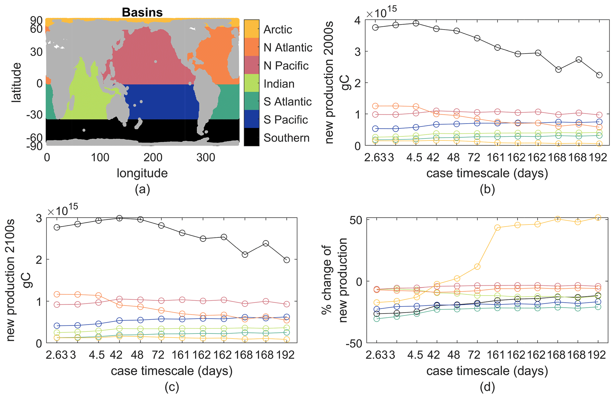
Figure B1(a) Map of the seven basins; colors are consistent through all panels. (b) Annual new production in the top 100 m in each basin for the early-21st-century climate. (c) As in (b) but for the late-21st-century climate. (d) Percent change between panels (a) and (b). The case timescale is . The fast case is the second from the left, case timescale 3. The slow case is the fourth from the right, case timescale 162.
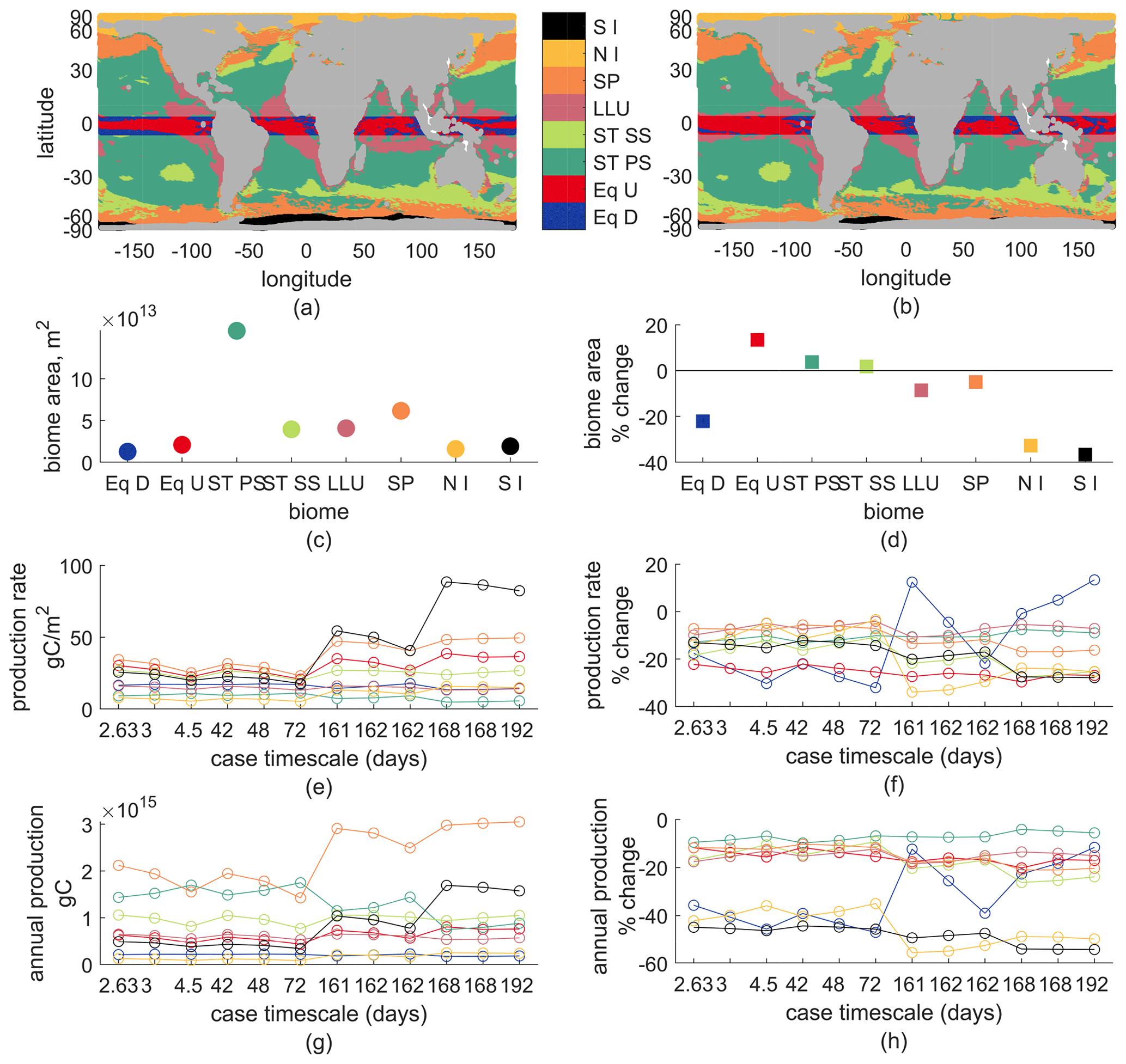
Figure B2(a) Biomes for 2000, (b) biomes for 2100, (c) biome areas for 2000, (d) percent change in biome area – early–late-21st-century, (e) production rate – annual gC/m2 for each biome (color) and each biogeochemical model parameter (x axis, case timescale). (f) Percent change in production rate. (g) Total annual production for each biome and biogeochemical model parameter, which is c⋅e. (h) Percent change in total annual production.
Data to reproduce the figures are available from Brett (2020a) (https://doi.org/10.5281/zenodo.4361701, last access: 11 May 2021). Code to reproduce the figures and to run these idealized tracers in CESM available from Brett (2020b) (https://doi.org/10.5281/zenodo.4361705, last access: 11 May 2021).
GJB designed and implemented the biogeochemical model. DBW and FB designed the physical model's time slice method, which was implemented by DBW. GJB, MCL, and FB designed the experiments. GJB performed the analyses with input from all coauthors. GJB wrote the initial draft. All coauthors contributed to edits of the writing, with substantial rewrites by DBW and MCL.
The authors declare that they have no conflict of interest.
Discussions with Keith Lindsay on the model implementation and Andy Thompson on study design are gratefully acknowledged. The CESM project is supported primarily by the National Science Foundation (NSF). This material is based upon work supported by the National Center for Atmospheric Research, which is a major facility sponsored by the NSF under cooperative agreement no. 1852977. Computing and data storage resources, including the Cheyenne supercomputer (https://doi.org/10.5065/D6RX99HX), were provided by the Computational and Information Systems Laboratory (CISL) at NCAR. We thank all the scientists, software engineers, and administrators who contributed to the development of CESM. Daniel B. Whitt also acknowledges support from NOAA (NA18OAR4310408) and NASA (80NSSC19K1116).
This work is funded by the National Science Foundation (NSF) under grants OCE-1658550 and OCE-1658541.
This paper was edited by Caroline P. Slomp and reviewed by two anonymous referees.
Alexander, M. A., Scott, J. D., Friedland, K. D., Mills, K. E., Nye, J. A., Pershing, A. J., and Thomas, A. C.: Projected sea surface temperatures over the 21st century: Changes in the mean, variability and extremes for large marine ecosystem regions of Northern Oceans, Elem. Sci. Anth., 6, https://doi.org/10.1525/elementa.191, 2018. a
Anugerahanti, P., Roy, S., and Haines, K.: Perturbed biology and physics signatures in a 1-D ocean biogeochemical model ensemble, Front. Mar. Sci., 7, https://doi.org/10.3389/fmars.2020.00549, 2020. a
Behrenfeld, M. J. and Boss, E. S.: Resurrecting the ecological underpinnings of ocean plankton blooms, Annu. Rev. Mar. Sci., 6, 167–194, 2014. a
Bopp, L., Resplandy, L., Orr, J. C., Doney, S. C., Dunne, J. P., Gehlen, M., Halloran, P., Heinze, C., Ilyina, T., Séférian, R., Tjiputra, J., and Vichi, M.: Multiple stressors of ocean ecosystems in the 21st century: projections with CMIP5 models, Biogeosciences, 10, 6225–6245, https://doi.org/10.5194/bg-10-6225-2013, 2013. a
Boyce, D. G., Lewis, M. R., and Worm, B.: Global phytoplankton decline over the past century, Nature, 466, 591–596, 2010. a
Brett, G.: Data, Sensitivity of 21st-century projected ocean new production changes to idealized biogeochemical model structure, https://doi.org/10.5281/zenodo.4361701, 2020a. a
Brett, G.: gjayb/CESMtracer v1.0 (Version v1.0), https://doi.org/10.5281/zenodo.4361705, 2020b. a
Cabré, A., Marinov, I., and Leung, S.: Consistent global responses of marine ecosystems to future climate change across the IPCC AR5 earth system models, Clim. Dynam., 45, 1253–1280, 2015. a, b, c, d
Danabasoglu, G., Lamarque, J.-F., Bacmeister, J., Bailey, D., DuVivier, A., Edwards, J., Emmons, L., Fasullo, J., Garcia, R., Gettelman, A., C. Hannay Holland, M. M., Large, W. G. Lauritzen, P. H. Lawrence, D. M. Lenaerts, J. T. M. Lindsay, K. Lipscomb, W. H. Mills, M. J. Neale, R. Oleson, K. W. Otto-Bliesner, B. Phillips, A. S. Sacks, W. Tilmes, S. van Kampenhout, L. Vertenstein, M. Bertini, A. Dennis, J. Deser, C. Fischer, C. Fox-Kemper, B. Kay, J. E. Kinnison, D. Kushner, P. J. Larson, V. E. Long, M. C. Mickelson, S. Moore, J. K. Nienhouse, E. Polvani, L. Rasch, P. J., and Strand, W. G.: The community earth system model version 2 (CESM2), J. Adv. Model. Earth Sy., 12, https://doi.org/10.1029/2019MS001916, 2020. a
Dasgupta, S., Singh, R. P., and Kafatos, M.: Comparison of global chlorophyll concentrations using MODIS data, Adv. Space Res., 43, 1090–1100, 2009. a
Deser, C., Hurrell, J. W., and Phillips, A. S.: The role of the North Atlantic Oscillation in European climate projections, Clim. Dynam., 49, 3141–3157, 2017. a
Eppley, R. W. and Peterson, B. J.: Particulate organic matter flux and planktonic new production in the deep ocean, Nature, 282, 677–680, 1979. a, b
Friedrichs, M. A., Hood, R. R., and Wiggert, J. D.: Ecosystem model complexity versus physical forcing: Quantification of their relative impact with assimilated Arabian Sea data, Deep-Sea Res. Pt. II, 53, 576–600, 2006. a
Fu, W., Randerson, J. T., and Moore, J. K.: Climate change impacts on net primary production (NPP) and export production (EP) regulated by increasing stratification and phytoplankton community structure in the CMIP5 models, Biogeosciences, 13, 5151–5170, https://doi.org/10.5194/bg-13-5151-2016, 2016. a, b, c
Galbraith, E. D., Dunne, J. P., Gnanadesikan, A., Slater, R. D., Sarmiento, J. L., Dufour, C. O., De Souza, G. F., Bianchi, D., Claret, M., Rodgers, K. B., and Marvasti, S. S.: Complex functionality with minimal computation: Promise and pitfalls of reduced-tracer ocean biogeochemistry models, J. Adv. Model. Earth Sy., 7, 2012–2028, https://doi.org/10.1002/2015MS000463, 2015. a
Garcia, H. E., Locarnini, R. A., Boyer, T. P., Antonov, J. I., Baranova, O. K., Zweng, M. M., Reagan, J. R., Johnson, D. R., Mishonov, A. V., and Levitus, S.: World ocean atlas 2013, edited by: Levitus, S. and Mishonov, A., Volume 4, Dissolved inorganic nutrients (phosphate, nitrate, silicate) [dataset], NOAA Atlas NESDIS 76, 25 pp., https://doi.org/10.7289/V5J67DWD, https://doi.org/10.7289/V5F769GT, 2013. a, b
Gent, P. R., Willebrand, J., McDougall, T. J., and McWilliams, J. C.: Parameterizing eddy-induced tracer transports in ocean circulation models, J. Phys. Oceanogr., 25, 463–474, 1995. a
Glessmer, M. S., Oschlies, A., and Yool, A.: Simulated impact of double-diffusive mixing on physical and biogeochemical upper ocean properties, J. Geophys. Res.-Oceans, 113, https://doi.org/10.1029/2007JC004455, 2008. a
Jackson, G. A. and Burd, A. B.: Aggregation in the marine environment, Environ. Sci. Technol., 32, 2805–2814, 1998. a
Kay, J. E., Deser, C., Phillips, A., Mai, A., Hannay, C., Strand, G., Arblaster, J. M., Bates, S., Danabasoglu, G., Edwards, J., Holland, M., Kushner, P., Lamarque, J.-F., Lawrence, D., Lindsay, K., Middleton, A., Munoz, E., Neale, R., Oleson, K., Polvani, L., and Vertenstein, M.: The Community Earth System Model (CESM) large ensemble project: A community resource for studying climate change in the presence of internal climate variability, B. Am. Meteorol. Soc., 96, 1333–1349, 2015. a
Knutti, R. and Sedláček, J.: Robustness and uncertainties in the new CMIP5 climate model projections, Nat. Clim. Change, 3, 369–373, 2013. a
Kriest, I.: Calibration of a simple and a complex model of global marine biogeochemistry, Biogeosciences, 14, 4965–4984, https://doi.org/10.5194/bg-14-4965-2017, 2017. a
Kriest, I. and Oschlies, A.: MOPS-1.0: towards a model for the regulation of the global oceanic nitrogen budget by marine biogeochemical processes, Geosci. Model Dev., 8, 2929–2957, https://doi.org/10.5194/gmd-8-2929-2015, 2015. a
Kriest, I., Oschlies, A., and Khatiwala, S.: Sensitivity analysis of simple global marine biogeochemical models, Global Biogeochem. Cy., 26, https://doi.org/10.1029/2011GB004072, 2012. a, b
Kriest, I., Kähler, P., Koeve, W., Kvale, K., Sauerland, V., and Oschlies, A.: One size fits all? Calibrating an ocean biogeochemistry model for different circulations, Biogeosciences, 17, 3057–3082, https://doi.org/10.5194/bg-17-3057-2020, 2020. a
Kvale, K. F. and Meissner, K. J.: Primary production sensitivity to phytoplankton light attenuation parameter increases with transient forcing, Biogeosciences, 14, 4767–4780, https://doi.org/10.5194/bg-14-4767-2017, 2017. a
Kwiatkowski, L., Torres, O., Bopp, L., Aumont, O., Chamberlain, M., Christian, J. R., Dunne, J. P., Gehlen, M., Ilyina, T., John, J. G., Lenton, A., Li, H., Lovenduski, N. S., Orr, J. C., Palmieri, J., Santana-Falcón, Y., Schwinger, J., Séférian, R., Stock, C. A., Tagliabue, A., Takano, Y., Tjiputra, J., Toyama, K., Tsujino, H., Watanabe, M., Yamamoto, A., Yool, A., and Ziehn, T.: Twenty-first century ocean warming, acidification, deoxygenation, and upper-ocean nutrient and primary production decline from CMIP6 model projections, Biogeosciences, 17, 3439–3470, https://doi.org/10.5194/bg-17-3439-2020, 2020. a, b
Kwon, E. Y. and Primeau, F.: Optimization and sensitivity study of a biogeochemistry ocean model using an implicit solver and in situ phosphate data, Global Biogeochem. Cy., 20, https://doi.org/10.1029/2005GB002631, 2006. a
Kwon, E. Y. and Primeau, F.: Optimization and sensitivity of a global biogeochemistry ocean model using combined in situ DIC, alkalinity, and phosphate data, J. Geophys. Res.-Oceans, 113, https://doi.org/10.1029/2007JC004520, 2008. a
Large, W. G. and Yeager, S. G.: Diurnal to decadal global forcing for ocean and sea-ice models: The data sets and flux climatologies, 2004. a, b
Large, W. G., Danabasoglu, G., Doney, S. C., and McWilliams, J. C.: Sensitivity to surface forcing and boundary layer mixing in a global ocean model: Annual-mean climatology, J. Phys. Oceanogr., 27, 2418–2447, 1997. a, b
Levy, M.: Exploration of the critical depth hypothesis with a simple NPZ model, ICES J. Mar. Sci., 72, 1916–1925, 2015. a, b
Llort, J., Lévy, M., Sallée, J.-B., and Tagliabue, A.: Nonmonotonic response of primary production and export to changes in mixed-layer depth in the Southern Ocean, Geophys. Res. Lett., 46, 3368–3377, 2019. a
Löptien, U. and Dietze, H.: Reciprocal bias compensation and ensuing uncertainties in model-based climate projections: pelagic biogeochemistry versus ocean mixing, Biogeosciences, 16, 1865–1881, https://doi.org/10.5194/bg-16-1865-2019, 2019. a
McGillicuddy Jr, D., Anderson, L., Doney, S., and Maltrud, M.: Eddy-driven sources and sinks of nutrients in the upper ocean: Results from a 0.1 resolution model of the North Atlantic, Global Biogeochem. Cy., https://doi.org/10.1029/2002GB001987, 17, 2003. a, b
Moore, J. K., Lindsay, K., Doney, S. C., Long, M. C., and Misumi, K.: Marine ecosystem dynamics and biogeochemical cycling in the Community Earth System Model [CESM1 (BGC)]: Comparison of the 1990s with the 2090s under the RCP4.5 and RCP8.5 scenarios, J. Climate, 26, 9291–9312, 2013. a, b
Najjar, R. G., Jin, X., Louanchi, F., Aumont, O., Caldeira, K., Doney, S. C., Dutay, J.-C., Follows, M., Gruber, N., Joos, F., Lindsay, K., Maier-Reimer, E., Matear, R. J., Matsumoto, K. Monfray, P. Mouchet, A. Orr, J. C. Plattner, G.-K. Sarmiento, J. L. Schlitzer, R. Slater, R. D. Weirig, M.-F. Yamanaka, Y. and Yool, A.: Impact of circulation on export production, dissolved organic matter, and dissolved oxygen in the ocean: Results from Phase II of the Ocean Carbon-cycle Model Intercomparison Project (OCMIP-2), Global Biogeochem. Cy., 21, https://doi.org/10.1029/2006GB002857, 2007. a
Oschlies, A.: Robustness and Uncertainties of Current Marine Carbon Cycle Models, Nova Acta Leopoldina, 121, 171–173, 2015. a
Pasquero, C., Bracco, A., and Provenzale, A.: Impact of the spatiotemporal variability of the nutrient flux on primary productivity in the ocean, J. Geophys. Res.-Oceans, 110, https://doi.org/10.1029/2004JC002738, 2005. a
Prieur, C., Viry, L., Blayo, E., and Brankart, J.-M.: A global sensitivity analysis approach for marine biogeochemical modeling, Ocean Modell., 139, 101402, https://doi.org/10.1016/j.ocemod.2019.101402, 2019. a
Redi, M. H.: Oceanic isopycnal mixing by coordinate rotation, J. Phys. Oceanogr., 12, 1154–1158, 1982. a
Romanou, A., Romanski, J., and Gregg, W. W.: Natural ocean carbon cycle sensitivity to parameterizations of the recycling in a climate model, Biogeosciences, 11, 1137–1154, https://doi.org/10.5194/bg-11-1137-2014, 2014. a
Sarmiento, J. L., Slater, R., Barber, R., Bopp, L., Doney, S. C., Hirst, A., Kleypas, J., Matear, R., Mikolajewicz, U., Monfray, P., Soldatov, V., Spall, S. A., and Stouffer, R.: Response of ocean ecosystems to climate warming, Global Biogeochem. Cy., 18, https://doi.org/10.1029/2003GB002134, 2004. a
Séférian, R., Bopp, L., Gehlen, M., Orr, J. C., Ethé, C., Cadule, P., Aumont, O., Mélia, D. S., Voldoire, A., and Madec, G.: Skill assessment of three earth system models with common marine biogeochemistry, Clim. Dynam., 40, 2549–2573, 2013. a
Séférian, R., Berthet, S., Yool, A., Palmieri, J., Bopp, L., Tagliabue, A., Kwiatkowski, L., Aumont, O., Christian, J., Dunne, J., Gehlen, M., Ilyina, T., John, J. G., Li, H., Long, M. C., Luo, J. Y., Nakano, H., Romanou, A., Schwinger, J., Stock, C., Santana-Falcón, Y., Takano, Y., Tjiputra, J., Tsujino, H., Watanabe, M., Wu, T., Wu, F., and Yamamoto, A.: Tracking improvement in simulated marine biogeochemistry between CMIP5 and CMIP6, Current Climate Change Reports, 1–25, https://doi.org/10.1007/s40641-020-00160-0, 2020. a
Sinha, B., Buitenhuis, E. T., Le Quéré, C., and Anderson, T. R.: Comparison of the emergent behavior of a complex ecosystem model in two ocean general circulation models, Prog. Oceanogr., 84, 204–224, 2010. a
Smith, K. M., Hamlington, P. E., and Fox-Kemper, B.: Effects of submesoscale turbulence on ocean tracers, J. Geophys. Res.-Oceans, 121, 908–933, 2016. a
Vancoppenolle, M., Bopp, L., Madec, G., Dunne, J., Ilyina, T., Halloran, P. R., and Steiner, N.: Future Arctic Ocean primary productivity from CMIP5 simulations: Uncertain outcome, but consistent mechanisms, Global Biogeochem. Cy., 27, 605–619, 2013. a, b
Yao, W., Kvale, K. F., Achterberg, E., Koeve, W., and Oschlies, A.: Hierarchy of calibrated global models reveals improved distributions and fluxes of biogeochemical tracers in models with explicit representation of iron, Environ. Res. Lett., 14, 114009, https://doi.org/10.1088/1748-9326/ab4c52, 2019. a