


1. Introduction
The observable signature of merging binary neutron stars (BNS) was revealed for the first time by the event GW170817, which started with a gravitational-wave (GW) chirp signal detected by the Advanced LIGO/Virgo detectors and was then followed by electromagnetic (EM) observations over a broad range of wavelengths from
 $\gamma$
-rays to radio (Abbott et al. Reference Abbott2017a, Reference Abbott2017b). One of the most promising outcomes is luminous EM emission in the optical and near-infrared bands after the final coalescence of the stars (e.g. Andreoni et al. Reference Andreoni2017; Arcavi et al. Reference Arcavi2017; Coulter et al. Reference Coulter2017; Cowperthwaite et al. Reference Cowperthwaite2017; Drout et al. Reference Drout2017; Kilpatrick et al. Reference Kilpatrick2017; Kasliwal et al. Reference Kasliwal2017; Smartt et al. Reference Smartt2017). This fast-evolving transient, referred to as a kilonova, was predicted to be powered by the radioactive decay of heavy elements via rapid neutron capture processes (Li & Paczyński Reference Li and Paczyński1998; Metzger et al. Reference Metzger2010; Barnes & Kasen Reference Barnes and Kasen2013; Tanaka & Hotokezaka Reference Tanaka and Hotokezaka2013; Fernández & Metzger Reference Fernández and Metzger2016). We now know that rapid EM follow-up (on the timescale of hours) provides a wealth of information on the nature of the progenitor (Abbott et al. Reference Abbott2017c; Kruckow et al. Reference Kruckow, Tauris, Langer, Kramer and Izzard2018), its environment (Levan et al. Reference Levan2017; Adhikari et al. Reference Adhikari, Fishbach, Holz, Wechsler and Fang2020), and explosion mechanism (Troja et al. Reference Troja2017; Mooley et al. Reference Mooley2018). In particular, the spectral evolution of such events is key to understanding the merger process and the origin of rare heavy elements (Kasen et al. Reference Kasen, Metzger, Barnes, Quataert and Ramirez-Ruiz2017; Kasliwal et al. Reference Kasliwal2019; Wu et al. Reference Wu, Barnes, Martínez-Pinedo and Metzger2019). Furthermore, the identification of an EM counterpart is needed to pinpoint the host galaxy, thus determining the redshift (Coulter et al. Reference Coulter2017; Hjorth et al. Reference Hjorth2017).
$\gamma$
-rays to radio (Abbott et al. Reference Abbott2017a, Reference Abbott2017b). One of the most promising outcomes is luminous EM emission in the optical and near-infrared bands after the final coalescence of the stars (e.g. Andreoni et al. Reference Andreoni2017; Arcavi et al. Reference Arcavi2017; Coulter et al. Reference Coulter2017; Cowperthwaite et al. Reference Cowperthwaite2017; Drout et al. Reference Drout2017; Kilpatrick et al. Reference Kilpatrick2017; Kasliwal et al. Reference Kasliwal2017; Smartt et al. Reference Smartt2017). This fast-evolving transient, referred to as a kilonova, was predicted to be powered by the radioactive decay of heavy elements via rapid neutron capture processes (Li & Paczyński Reference Li and Paczyński1998; Metzger et al. Reference Metzger2010; Barnes & Kasen Reference Barnes and Kasen2013; Tanaka & Hotokezaka Reference Tanaka and Hotokezaka2013; Fernández & Metzger Reference Fernández and Metzger2016). We now know that rapid EM follow-up (on the timescale of hours) provides a wealth of information on the nature of the progenitor (Abbott et al. Reference Abbott2017c; Kruckow et al. Reference Kruckow, Tauris, Langer, Kramer and Izzard2018), its environment (Levan et al. Reference Levan2017; Adhikari et al. Reference Adhikari, Fishbach, Holz, Wechsler and Fang2020), and explosion mechanism (Troja et al. Reference Troja2017; Mooley et al. Reference Mooley2018). In particular, the spectral evolution of such events is key to understanding the merger process and the origin of rare heavy elements (Kasen et al. Reference Kasen, Metzger, Barnes, Quataert and Ramirez-Ruiz2017; Kasliwal et al. Reference Kasliwal2019; Wu et al. Reference Wu, Barnes, Martínez-Pinedo and Metzger2019). Furthermore, the identification of an EM counterpart is needed to pinpoint the host galaxy, thus determining the redshift (Coulter et al. Reference Coulter2017; Hjorth et al. Reference Hjorth2017).
Photometric and spectroscopic data of kilonovae provide a novel probe into the physics and nature of the BNS themselves (e.g. NS radius or mass ratio) and into the process and end-product of mergers. Although GW170817 remains the only kilonova that was both spectroscopically confirmed and associated with a GW signal, it allows us to better understand how different ejecta components (with different lanthanide fractions) contribute its EM emission from early to late times after the merger. However, little is known about the earliest stages of the kilonova, because the EM coverage of GW170817 started more than 10 h after the event. Hence, we have no constraints yet on possible emission from the outermost layers of the ejecta that may have faded after a few hours. For example, Metzger et al. (Reference Metzger, Bauswein, Goriely and Kasen2015) proposed a candidate precursor of kilonova emission, caused by
 $\beta$
-decay of free neutrons in the outermost ejecta, which can increase the luminosity of the EM source by over an order of magnitude during the first hour after the merger. Metzger (Reference Metzger2019) mentions r-process heating or radioactive decay of free neutrons. And further mechanisms such as jet/wind reheating could play a similar role in producing enhanced luminosity at early times (e.g. Metzger, Thompson, & Quataert Reference Metzger, Thompson and Quataert2018). Only high-cadence observations in the first few hours after the merger can test these predictions in detail and reveal the source of the blue emission (Arcavi Reference Arcavi2018).
$\beta$
-decay of free neutrons in the outermost ejecta, which can increase the luminosity of the EM source by over an order of magnitude during the first hour after the merger. Metzger (Reference Metzger2019) mentions r-process heating or radioactive decay of free neutrons. And further mechanisms such as jet/wind reheating could play a similar role in producing enhanced luminosity at early times (e.g. Metzger, Thompson, & Quataert Reference Metzger, Thompson and Quataert2018). Only high-cadence observations in the first few hours after the merger can test these predictions in detail and reveal the source of the blue emission (Arcavi Reference Arcavi2018).
The SkyMapper optical wide-field telescope in Australia (see Section 2.1) is one of the facilities that can discover early GW170817-like kilonovae and is probably the pivotal optical facility for events that occur in the Southern Sky between the end of the Chilean night and late in the Australian night. The size of the GW localisation area (a few hundred deg
 $^2$
, see Abbott et al. Reference Abbott2020a) is usually much larger than the field of view (FoV) of our camera (
$^2$
, see Abbott et al. Reference Abbott2020a) is usually much larger than the field of view (FoV) of our camera (
 $5.7\, \mathrm{deg}^2$
). While the GW triggers in the third LIGO/Virgo observing run (O3) had a median localisation area of
$5.7\, \mathrm{deg}^2$
). While the GW triggers in the third LIGO/Virgo observing run (O3) had a median localisation area of
 $4\,480\, \mathrm{deg}^2$
(Kasliwal et al. Reference Kasliwal2020), the area shrinks quickly for events with stronger signals. A synoptic tiling strategy covering the high-probability sky area for the counterpart will usually best exploit our wide FoV, and our tiles follow the basic tiling scheme of the general-purpose SkyMapper Southern Survey (Onken et al. Reference Onken2019, see Section 2.1). In contrast, an alternative galaxy-targeted approach makes more sense for telescopes with smaller FoV and for nearby events such as GW170817, where it has proven to be effective. However, for events at distance larger than 50 Mpc, which are expected to be by far the most common, our FoV contains usually several possible host galaxies and empty tiles will be rare. Crucially, we can detect transient candidates in real time as we have reference images for subtraction over the full hemisphere (at least in some passbands, see Section 2.3.2), which are deep enough to detect GW170817-like kilonovae at distances up to 200 Mpc as well as the rising part of kilonova light curves in more nearby cases.
$4\,480\, \mathrm{deg}^2$
(Kasliwal et al. Reference Kasliwal2020), the area shrinks quickly for events with stronger signals. A synoptic tiling strategy covering the high-probability sky area for the counterpart will usually best exploit our wide FoV, and our tiles follow the basic tiling scheme of the general-purpose SkyMapper Southern Survey (Onken et al. Reference Onken2019, see Section 2.1). In contrast, an alternative galaxy-targeted approach makes more sense for telescopes with smaller FoV and for nearby events such as GW170817, where it has proven to be effective. However, for events at distance larger than 50 Mpc, which are expected to be by far the most common, our FoV contains usually several possible host galaxies and empty tiles will be rare. Crucially, we can detect transient candidates in real time as we have reference images for subtraction over the full hemisphere (at least in some passbands, see Section 2.3.2), which are deep enough to detect GW170817-like kilonovae at distances up to 200 Mpc as well as the rising part of kilonova light curves in more nearby cases.
In the O3 run, 56 gravitational-wave events from compact binary systems were detected, which is 5 times more than reported during the first two observing runs. Only two of them had significant (
 $>85\%$
) initial probability of being BNS events: S190425z (LIGO Scientific Collaboration & VIRGO Collaboration, Reference Scientific Collaboration2019) and S190901ap (LIGO Scientific Collaboration & Virgo Collaboration, Reference Scientific Collaboration2019). However, after reanalysis with background statistics the latter is no longer considered a significant candidate (Abbott et al. Reference Abbott2020c). S190425z, a.k.a. GW190425 and known in Australia as the ANZAC Day event, was also confirmed as the second case of gravitational waves from a binary neutron star inspiral (Abbott et al. Reference Abbott2020b). The system is noteworthy for a total mass of
$>85\%$
) initial probability of being BNS events: S190425z (LIGO Scientific Collaboration & VIRGO Collaboration, Reference Scientific Collaboration2019) and S190901ap (LIGO Scientific Collaboration & Virgo Collaboration, Reference Scientific Collaboration2019). However, after reanalysis with background statistics the latter is no longer considered a significant candidate (Abbott et al. Reference Abbott2020c). S190425z, a.k.a. GW190425 and known in Australia as the ANZAC Day event, was also confirmed as the second case of gravitational waves from a binary neutron star inspiral (Abbott et al. Reference Abbott2020b). The system is noteworthy for a total mass of
 $3.4\,{\rm M}_{\odot}$
, which exceeds that of known Galactic BNS and may suggest that not all all binary neutron stars are formed in the same way (Romero-Shaw et al. Reference Romero-Shaw, Farrow, Stevenson, Thrane and Zhu2020, Safarzadeh, Ramirez-Ruiz, & Berger Reference Safarzadeh, Ramirez-Ruiz and Berger2020). No EM counterpart was found by SkyMapper or any other facility, because (i) the sky localisation of this event was poorly constrained with a 90% confidence area of
$3.4\,{\rm M}_{\odot}$
, which exceeds that of known Galactic BNS and may suggest that not all all binary neutron stars are formed in the same way (Romero-Shaw et al. Reference Romero-Shaw, Farrow, Stevenson, Thrane and Zhu2020, Safarzadeh, Ramirez-Ruiz, & Berger Reference Safarzadeh, Ramirez-Ruiz and Berger2020). No EM counterpart was found by SkyMapper or any other facility, because (i) the sky localisation of this event was poorly constrained with a 90% confidence area of
 $8\,284\, \mathrm{deg}^{2}$
, (ii) it is expected to be much fainter than GW170817 in the optical due to its distance, and (iii) it may be intrinsically faint due to a low ejecta mass or unfavourable viewing angle. In preparation for the next LIGO/Virgo observing run (O4), we describe here our facility and its performance with the current processing pipeline.
$8\,284\, \mathrm{deg}^{2}$
, (ii) it is expected to be much fainter than GW170817 in the optical due to its distance, and (iii) it may be intrinsically faint due to a low ejecta mass or unfavourable viewing angle. In preparation for the next LIGO/Virgo observing run (O4), we describe here our facility and its performance with the current processing pipeline.
For an autonomous selection of transient candidates, it is key to maximise the recovery rate and minimise the false-positive rate; in order to reduce the volume of human intervention required to identify the likely source of interest, on which detailed follow-up observations may be triggered. This process faces two challenges: (1) Image artefacts appear in the subtraction process and pose as transient candidates; this is often addressed with machine learning approaches that separate astrophysical sources from spurious detections in a difference image (e.g. Bailey et al. Reference Bailey, Aragon, Romano, Thomas, Weaver and Wong2007; Bloom et al. Reference Bloom2012; Brink et al. Reference Brink, Richards, Poznanski, Bloom, Rice, Negahban and Wainwright2013; Wright et al. Reference Wright2015; Goldstein et al. Reference Goldstein2015; Duev et al. Reference Duev2019). (2) Astrophysical foreground and background transients produce a fog of events that are not related to the GW event, and these are usually too numerous for simultaneous follow-up. In this work, we use an ensemble-based transient classifier to reject spurious sources and refer to catalogues of known sources to label other types of variables.
In this paper, we present an overview of the SkyMapper follow-up programme of GW triggers. In Section 2, we describe our optical facility and the AlertSDP pipeline in detail, from observing strategy to real-time data processing and transient identification. In Section 3, we introduce an ensemble-based machine learning approach for real-bogus classification. We also present metrics for evaluating the performance of the classifier. In Section 4, we present a real case and discuss the resulting transient statistics. In Section 5, we close with an outlook to future work and the LIGO/Virgo O4 run. Throughout the paper we use the AB magnitude system.
2. EM counterpart searches with the SkyMapper facility
2.1. SkyMapper telescope
SkyMapper is a 1.35 m modified Cassegrain telescope located at Siding Spring Observatory (SSO) in New South Wales, Australia (Wolf et al. Reference Wolf2018). The telescope has a wide field of view of
 $2.34 \times 2.37\, \mathrm{deg}^2$
, a uvgriz filter set (Bessell et al. Reference Bessell, Bloxham, Schmidt, Keller, Tisserand and Francis2011) and a mosaic of 32
$2.34 \times 2.37\, \mathrm{deg}^2$
, a uvgriz filter set (Bessell et al. Reference Bessell, Bloxham, Schmidt, Keller, Tisserand and Francis2011) and a mosaic of 32
 $2\mathrm{k}\times4\mathrm{k}$
CCD detectors with a pixel scale of
$2\mathrm{k}\times4\mathrm{k}$
CCD detectors with a pixel scale of
 $0.5 \mathrm{arcsec pixel}^{-1}$
. It is owned and operated by the Australian National University (ANU) and, most importantly for EM follow-up, it is a robotic facility.
$0.5 \mathrm{arcsec pixel}^{-1}$
. It is owned and operated by the Australian National University (ANU) and, most importantly for EM follow-up, it is a robotic facility.
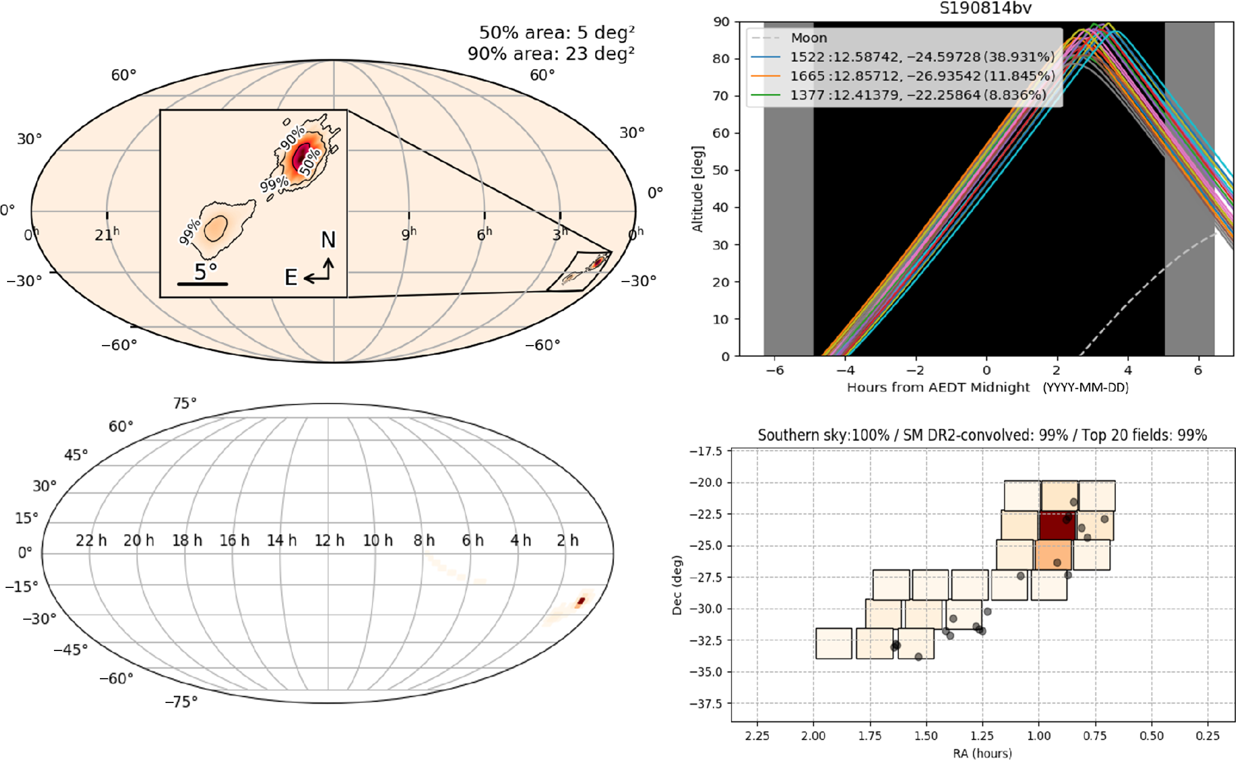
Figure 1. Top left: LIGO/Virgo probability sky map for S190814bv produced with the ligo.skymap module (Singer et al. Reference Singer2016). The inset shows the most probable area for the optical counterpart. Darker colours correspond to higher probability sky regions, and contours enclosing regions with 50%, 90%, and 99% of the probability are indicated. Bottom left: probability map convolved with the coverage of reference images in SkyMapper DR2. Bottom right: zoomed-in map of the 20 highest-probability fields selected for the search; here, one field alone has
 $\sim 39\%$
probability of containing the GW source. Symbols are bright galaxies from the 2MASS redshift survey. Top right: Observability plot for the top 20 fields with telescope altitude, night-time range and Moon separation.
$\sim 39\%$
probability of containing the GW source. Symbols are bright galaxies from the 2MASS redshift survey. Top right: Observability plot for the top 20 fields with telescope altitude, night-time range and Moon separation.
The main purpose of the telescope is the SkyMapper Southern Survey (SMSS), a hemispheric sky atlas which has been underway since 2014 (DR1: Wolf et al. Reference Wolf2018; DR2: Onken et al. Reference Onken2019). For point sources with
 $\mathrm{SNR}>5$
, the expected photometric depth of single-epoch 100-s images is u = 19.5, v = 19.5, g = 21, r = 20.5, i = 20, and z = 19 mag. Alongside, SkyMapper has been used to search for extragalactic transients, including low-redshift Type Ia supernovae (Scalzo et al. Reference Scalzo2017; Möller et al. Reference Griffin2019) as well as optical counterparts to GW events (GW170817: Abbott et al. Reference Abbott2017b; Andreoni et al. Reference Andreoni2017) and fast radio bursts (e.g. Petroff et al. Reference Petroff2015; Farah et al. Reference Farah2018; Reference Farah2019; Price et al. Reference Price2019; Chang et al. Reference Chang, Wolf, Onken, Luvaul, Gupta and Flynn2019a). Different needs made the SMSS and the transient searches develop separate data reduction software: the Science Data Pipeline (SDP: Luvaul et al. Reference Luvaul, Onken, Wolf, Smillie, Sebo, Lorente, Shortridge and Wayth2017; Wolf et al. Reference Wolf2018) for the SMSS and the Subtraction Pipeline (SUBPIPE; Scalzo et al. Reference Scalzo2017) for the Transient Survey. SUBPIPE was used for EM data analysis before before LIGO/Virgo ER14 (Engineering Run 14), but for the O3 run we updated it to an automated real-time pipeline (AlertSDP: Alert Science Data Pipeline) that borrows many features from the SDP (see Sections 2.2 and 2.3 for details).
$\mathrm{SNR}>5$
, the expected photometric depth of single-epoch 100-s images is u = 19.5, v = 19.5, g = 21, r = 20.5, i = 20, and z = 19 mag. Alongside, SkyMapper has been used to search for extragalactic transients, including low-redshift Type Ia supernovae (Scalzo et al. Reference Scalzo2017; Möller et al. Reference Griffin2019) as well as optical counterparts to GW events (GW170817: Abbott et al. Reference Abbott2017b; Andreoni et al. Reference Andreoni2017) and fast radio bursts (e.g. Petroff et al. Reference Petroff2015; Farah et al. Reference Farah2018; Reference Farah2019; Price et al. Reference Price2019; Chang et al. Reference Chang, Wolf, Onken, Luvaul, Gupta and Flynn2019a). Different needs made the SMSS and the transient searches develop separate data reduction software: the Science Data Pipeline (SDP: Luvaul et al. Reference Luvaul, Onken, Wolf, Smillie, Sebo, Lorente, Shortridge and Wayth2017; Wolf et al. Reference Wolf2018) for the SMSS and the Subtraction Pipeline (SUBPIPE; Scalzo et al. Reference Scalzo2017) for the Transient Survey. SUBPIPE was used for EM data analysis before before LIGO/Virgo ER14 (Engineering Run 14), but for the O3 run we updated it to an automated real-time pipeline (AlertSDP: Alert Science Data Pipeline) that borrows many features from the SDP (see Sections 2.2 and 2.3 for details).
2.2. Alert response
We continuously listen to the live stream of LIGO/Virgo public alerts for compact binary merger candidates.Footnote a The stream is distributed through the Gamma-ray Coordinates Network (GCN) using the pygcn Python module.Footnote b We developed a robotic alert handler that extracts relevant information, ingests the GW event into our database, downloads the HEALPix 3D localisation map (skymap), prioritises areas for follow-up, and generates a list of observations for SkyMapper.
The first preliminary GCN notice is automatically issued for a superevent within 1–10 min after the GW trigger. From this notice, our robotic handler initiates rapid-response search observations by convolving the probability in the BAYESTAR skymap (Singer & Price Reference Singer and Price2016) with the tile pattern of the SkyMapper Southern Survey (Onken et al. Reference Onken2019), ranking the fields by probability integrated per field and then selecting the top 20 fields with existing i-band reference images (
 $\sim100\, \mathrm{deg}^2$
total area). Figure 1 shows the sky maps for a real alert and an observability map of the selected target fields.
$\sim100\, \mathrm{deg}^2$
total area). Figure 1 shows the sky maps for a real alert and an observability map of the selected target fields.
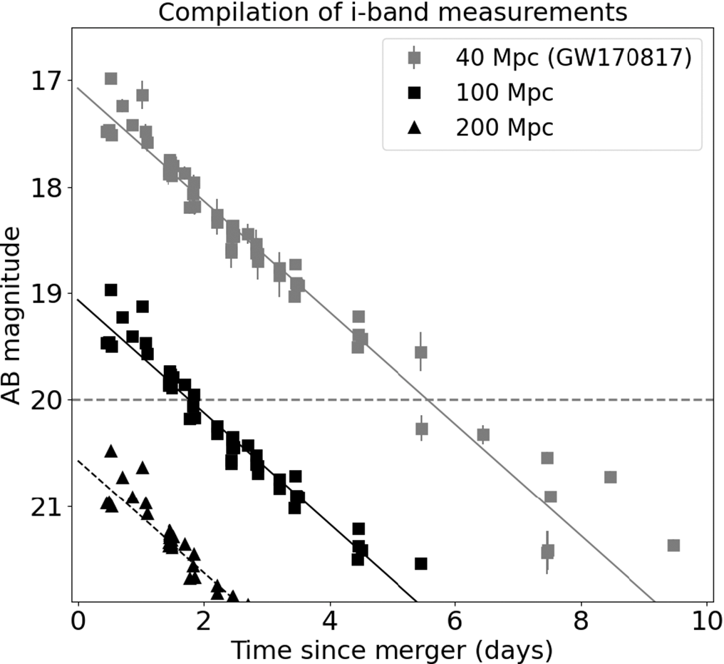
Figure 2. The i-band light curve for the GW170817 kilonova, at different distances: at the true distance of 40 Mpc (top), shifted to 100 Mpc (middle) and 200 Mpc (bottom); solid lines are power law decay fits. The dashed line at
 $i_{\textrm{AB}}=20$
marks our typical 5-
$i_{\textrm{AB}}=20$
marks our typical 5-
 $\sigma$
magnitude limit in 100 s exposures (data were taken from various literature sources; AST3-2: Hu et al. Reference Hu2017 ; B&C: Utsumi et al. Reference Utsumi2017; DECam: Cowperthwaite et al. Reference Cowperthwaite2017; Gemini: Kasliwal et al. Reference Kasliwal2017; LaSilla: Smartt et al. Reference Smartt2017; LCO: Arcavi et al. Reference Arcavi2017; Magellan: Shappee et al. Reference Shappee2017; Pan-STARRS: Smartt et al. Reference Smartt2017; REM: Pian et al. Reference Pian2017; SkyMapper: Andreoni et al. Reference Andreoni2017; Swope: Drout et al. Reference Drout2017;T80S: D az et al. 2017; VLT: Tanvir et al. Reference Tanvir2017; VST: Pian et al. Reference Pian2017).
$\sigma$
magnitude limit in 100 s exposures (data were taken from various literature sources; AST3-2: Hu et al. Reference Hu2017 ; B&C: Utsumi et al. Reference Utsumi2017; DECam: Cowperthwaite et al. Reference Cowperthwaite2017; Gemini: Kasliwal et al. Reference Kasliwal2017; LaSilla: Smartt et al. Reference Smartt2017; LCO: Arcavi et al. Reference Arcavi2017; Magellan: Shappee et al. Reference Shappee2017; Pan-STARRS: Smartt et al. Reference Smartt2017; REM: Pian et al. Reference Pian2017; SkyMapper: Andreoni et al. Reference Andreoni2017; Swope: Drout et al. Reference Drout2017;T80S: D az et al. 2017; VLT: Tanvir et al. Reference Tanvir2017; VST: Pian et al. Reference Pian2017).
In this search stage, we obtain two
 $100\,\mathrm{s}$
exposures in i-band for each field, separated by
$100\,\mathrm{s}$
exposures in i-band for each field, separated by
 $\sim 8\,\mathrm{min}$
. Requiring a twin detection in the two images eliminates moving objects from the candidate list. The typical rate of motion for main-belt asteroids, 0.625 arcsec
$\sim 8\,\mathrm{min}$
. Requiring a twin detection in the two images eliminates moving objects from the candidate list. The typical rate of motion for main-belt asteroids, 0.625 arcsec
 $\mathrm{min}^{-1}$
near opposition (Jedicke Reference Jedicke1996), provides a sufficient
$\mathrm{min}^{-1}$
near opposition (Jedicke Reference Jedicke1996), provides a sufficient
 $\sim 5$
arcsec spacing between observations. With a depth of
$\sim 5$
arcsec spacing between observations. With a depth of
 $i\approx 20\,\mathrm{mag}$
, we can identify kilonovae that are
$i\approx 20\,\mathrm{mag}$
, we can identify kilonovae that are
 $\sim 3\,\mathrm{mag} (16\times$
) fainter than the kilonova of GW170817 was 10 h after the GW trigger. Hence, we could detect kilonovae for GW170817-like events out to
$\sim 3\,\mathrm{mag} (16\times$
) fainter than the kilonova of GW170817 was 10 h after the GW trigger. Hence, we could detect kilonovae for GW170817-like events out to
 $4\times$
the distance of GW170817, or 160 Mpc. Figure 2 shows the lightcurve of the GW170817 kilonova shifted to different distances up to 200 Mpc. The declining nature of the i-band light curve suggests that kilonovae may be more luminous during the first 10 h. We thus assume that we might be able to detect early kilonova emission, just hours after a BNS merger, out to distances of 200 Mpc or beyond.
$4\times$
the distance of GW170817, or 160 Mpc. Figure 2 shows the lightcurve of the GW170817 kilonova shifted to different distances up to 200 Mpc. The declining nature of the i-band light curve suggests that kilonovae may be more luminous during the first 10 h. We thus assume that we might be able to detect early kilonova emission, just hours after a BNS merger, out to distances of 200 Mpc or beyond.
We search in i-band for three reasons: (i) kilonovae are expected to be red due to the large opacity of neutron-rich ejecta, although at early times (within an hour of the merger) blue emission from hotter, polar ejecta may be expected (e.g. Troja et al. Reference Troja2018), (ii) the i-band covers the largest sky area with deep reference images in the SMSS that can be used for real-time image subtraction, and therefore provides the greatest search volume for kilonovae, and (iii) the dominant source of transient events, flares on M stars too faint to be seen in quiescence, is nearly irrelevant in i-band (Chang, Wolf, & Onken Reference Chang, Wolf and Onken2020). The aim of the search phase is to find a counterpart as fast as possible, report it to facilities around the world and get SkyMapper itself into monitoring mode. We expect that the search phase provides a full set of possible counterparts within 4 h (limited by image processing) after the GW trigger, if the trigger occurs during darkness and the sky is clear. Later, possibly within 4 h for BNS or NSBH events, an updated LALInference skymap (Veitch et al. Reference Veitch2015) will be distributed, including an updated sky localisation and source classification. This sometimes leads to a significant change in the sky localisation, and the SkyMapper observing plan may be modified and re-executed as a result.
At any time, once a position of a likely kilonova transient is identified, we can manually switch from the search phase to a continuous high-cadence monitoring of the new source. Observations of an early kilonova with a cadence of 2 min would reveal structure in the lightcurve arising from shocks induced by the kilonova ejecta (e.g. Metzger Reference Metzger2019). We will also get high-cadence, multi-band light curves for several consecutive nights after any kilonova discovery. The monitoring strategy will change depending on the colour, luminosity, and fading timescale of the kilonova candidates. If the optical counterpart gets identified by other groups before SkyMapper can observe, we will do only light-curve monitoring, as was the case for GW170817 (Andreoni et al. Reference Andreoni2017).
2.3. AlertSDP: Alert science data pipeline
The AlertSDP is a new pipeline created from two existing software packages, which are the SkyMapper Science Data Pipeline, SDP, and SUBPIPE, which was used for discovering low-redshift supernovae (see Section 2.1). The SDP has provided the general process control framework as well as improved calibration and masking treatment, while the subtraction and transient classification have evolved from SUBPIPE components. First, each raw image is preprocessed and calibrated. After that, i-band reference images for image subtraction are selected, and transient candidates detected on difference images are uploaded into a database. The database also includes external catalogues to assist transient classification.
2.3.1. Ingest and calibration of new images
Raw SkyMapper images from Siding Spring Observatory are transferred in real time via Ethernet to a 64-core server at Mount Stromlo Observatory. Data transfer takes 5–7 s per frame and can be done while the next exposure is already being taken. To activate the AlertSDP, the Linux inotify mechanism detects the arrival of an image from the telescope immediately and initiates the data processing.
The raw data are processed into scientific data products using typical SDP procedures, including bias correction, flat-fielding, defringing, bad-pixel masking, and generation of an astrometric solution (see Wolf et al. Reference Wolf2018 and Onken et al. Reference Onken2019 for details). A significant structural change from the SDP to the AlertSDP is a different parallelisation paradigm designed to minimise the time between image acquisition and production of transient candidates: while the SDP processes images in parallel with all the component CCDs treated serially, the AlertSDP processes the 32 CCDs of each image in parallel and up to 4 images concurrently.
2.3.2. Selection of reference images
Reference images are required for image subtraction and real-time transient searching. We take advantage of the nearly all-Southern-sky coverage (
 $>\!98 \%$
) of the deeper Main Survey exposures from the SMSS in i-band (
$>\!98 \%$
) of the deeper Main Survey exposures from the SMSS in i-band (
 $\lambda_\mathrm{centre}/\Delta \lambda = 779/140 \mathrm{nm}$
). Figure 3 shows the area of sky covered by SkyMapper DR2 (Onken et al. Reference Onken2019) and by DR3, which was released to the Australian community in February 2020 in the late stages of the O3 run. DR3 expands the deep coverage by including survey observations from 2014 March to 2019 October.Footnote c
$\lambda_\mathrm{centre}/\Delta \lambda = 779/140 \mathrm{nm}$
). Figure 3 shows the area of sky covered by SkyMapper DR2 (Onken et al. Reference Onken2019) and by DR3, which was released to the Australian community in February 2020 in the late stages of the O3 run. DR3 expands the deep coverage by including survey observations from 2014 March to 2019 October.Footnote c
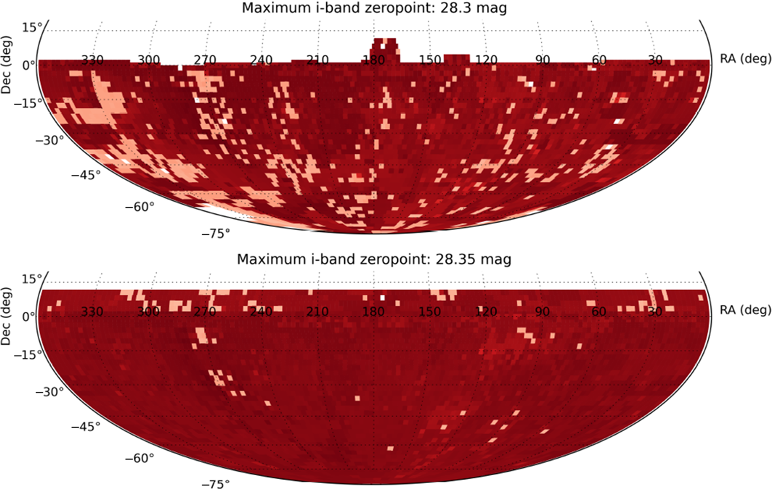
Figure 3. SkyMapper i band coverage in DR2 (top) and DR3 (bottom). Darker colours resemble deeper reference images used for subtraction.
From any new image, we subtract each available reference image. The best possible reference image combines a small PSF and a large overlap with the new image. The reference images come with a range of point-spread functions (PSF), and because the SMSS obtains repeat images with dithering to cover the sky homogeneously, the best-available reference PSF changes discontinuously with sky location. Small overlaps lead to badly determined convolution kernels and thus bad subtractions. Hence, we require at least 15% overlap area for mosaic frames and at least 5% overlap for each individual CCD. Following a common strategy of other transient surveys, we require that the reference image should be taken at least two weeks prior to a given new epoch.
2.3.3. Subtraction of images
We perform image subtraction on each field of overlapping new/reference image pairs. First, we resample each of the reference mosaic frames onto the new image with SWarp (Bertin et al. Reference Bertin, Mellier, Radovich, Missonnier, Didelon, Morin, Bohlender, Durand and Handley2002). Next, we convolve those pairs of images to a common PSF using HOTPANTS (Becker Reference Becker2015), which implemented the popular image subtraction algorithm by Alard & Lupton (Reference Alard and Lupton1998). Solving for the convolution kernel is a crucial step to equalising the PSFs of the reference and new images. The position-dependent PSF variation in both images is modelled as a linear combination of basis functions, and by default we choose a 2D polynomial of order two. Next, the flux level of the subtracted image is normalised to that of the reference image. Since the photometric calibration is directly tied to the SMSS photometry, this approach has the advantage of allowing explicit calculation of zero-point corrected magnitudes. The preliminary calibrated magnitude and error used for lightcurve construction is
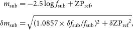 \begin{align} m_{\rm sub} &= -2.5 \log f_{\rm sub} + {\rm ZP_{\rm ref}}, \notag \\[4pt]
\delta m_{\rm sub} &= \sqrt{(1.0857 \times \delta f_{\rm sub}/f_{\rm sub} )^{2} + {\rm \delta ZP_{\rm ref}}^{2}}, \notag\end{align}
\begin{align} m_{\rm sub} &= -2.5 \log f_{\rm sub} + {\rm ZP_{\rm ref}}, \notag \\[4pt]
\delta m_{\rm sub} &= \sqrt{(1.0857 \times \delta f_{\rm sub}/f_{\rm sub} )^{2} + {\rm \delta ZP_{\rm ref}}^{2}}, \notag\end{align}
where
 ${f_{\rm sub}}$
is the difference flux on the subtracted image and
${f_{\rm sub}}$
is the difference flux on the subtracted image and
 ${\rm ZP_{\rm ref}}$
is the zeropoint of the reference image. Here, we use the 15 arcsec (30-pixel-diameter) aperture as a total-magnitude reference. The zeropoint error
${\rm ZP_{\rm ref}}$
is the zeropoint of the reference image. Here, we use the 15 arcsec (30-pixel-diameter) aperture as a total-magnitude reference. The zeropoint error
 $\delta {\rm ZP_{\rm ref}}$
contributes little, since only images with robust zeropoints are included in SMSS data releases.
$\delta {\rm ZP_{\rm ref}}$
contributes little, since only images with robust zeropoints are included in SMSS data releases.
Finally, we run SExtractor (Bertin & Arnouts Reference Bertin and Arnouts1996) on the subtracted images to produce a list of transient candidates and their associated metadata, using a low detection threshold of
 $1.5\sigma$
above the background. Gaussian filters in SExtractor are applied to an image prior to the detection of sources. Only sources with a signal-to-noise ratio below 2 are referred to as sub-threshold detections.
$1.5\sigma$
above the background. Gaussian filters in SExtractor are applied to an image prior to the detection of sources. Only sources with a signal-to-noise ratio below 2 are referred to as sub-threshold detections.
2.4. Transient classification
Until the end of O3, we classified transient candidates with a random forest (RF) classifier trained on earlier supernova survey data (Scalzo et al. Reference Scalzo2017). We computed a set of features derived from difference images of individual candidates, similar to those proposed in Bloom et al. (Reference Bloom2012). The main difference was that three additional checks were made on each candidate: (i) we removed any detections where the measurement of shape parameters (e.g. FWHM, elongation) was significantly larger than the median quantities for sources found in the new science images, and (ii) we matched each of them to the nearest object (
 $<30 \mathrm{arcsec}$
) seen on the reference frame, which will be associated with host galaxies or bright stars that might be poorly subtracted. Then, the RF model assigned a real-bogus score (RBscore) from 0 (artefacts = bogus) to 100 (transients = real) to all the detected candidates.
$<30 \mathrm{arcsec}$
) seen on the reference frame, which will be associated with host galaxies or bright stars that might be poorly subtracted. Then, the RF model assigned a real-bogus score (RBscore) from 0 (artefacts = bogus) to 100 (transients = real) to all the detected candidates.
In this work, we added a new classifier (XGBoost) and new training sets to exploit our improved image processing. A combination of classifiers is often more accurate than a single classifier, and thus we introduce a new metric (Tscore) that combines RBscore and XGBoost score to compensate for the weakness of each classifier (see Section 3 for the full description and performance).
For each transient candidate, we identify whether it may be a known variable or Milky Way source by cross-matching it against catalogues of stars, variable objects and quasars, using a 3 arcsec search radius. We also reject known solar system objects with the SkyBoT cone-search service (Berthier et al. Reference Berthier, Vachier, Thuillot, Fernique, Ochsenbein, Genova, Lainey, Arlot, Gabriel, Arviset, Ponz and Enrique2006). Our preselected categories are as follows:
-
• We define a ‘Star’ sample using parallaxes and proper motions (PPM) from Gaia eDR3 (Gaia Collaboration et al. Reference Gaia2016, Reference Gaia, Brown, Vallenari, Prusti, de Bruijne, Babusiaux and Biermann2020), requiring that the significance of a PPM signalFootnote d is
 $S_{\rm PPM}>3$
.
$S_{\rm PPM}>3$
. -
• For Gaia eDR3 objects with lower PPM SN or no PPM information, we use a ‘GaiaSource’ label.
-
• We use the label ‘Var’ for all sources cross-matched to the AAVSO International Variable Star Index (Watson, Henden, & Price Reference Watson, Henden and Price2006; version 2020 October 19). It contains mainly known variable stars and a few QSOs.
-
• We assign a label of ‘Quasar’ to sources matched to the Milliquas catalogue (Flesch Reference Flesch2015, version 7.0a).
-
• For detections that are too close to very bright stars and carry a risk of being an optical reflection (defined by the algorithm in item 3 of Section 2.6.1 from Onken et al. Reference Onken2019), we use a ‘BrightStar’ label.

In addition, image mask data allows us to reject sources as being likely spurious, when they could be affected by bad pixels, neighbouring saturated pixels, or cosmic ray hits. Only candidates with Tscore greater than 30 (see Section 3) are considered plausible candidates and presented for visual inspection. If the number of plausible sources in a single CCD image exceeds 50, we reject all detections in that CCD because the quality of subtracted image is likely to be poor.
2.5. Further follow-up mechanisms
We manage data sets of transient candidates, building on a web user interface developed by Scalzo et al. (Reference Scalzo2017) based on the Django framework. Following the initial automated typing of the candidates, the next step requires a human to visually inspect and classify the remaining candidates in a web interface. All plausible candidates are assigned a unique name. Since we visit any field at least twice during the search, we prioritise candidates in the visual examination that are detected at least twice. We keep a list of ‘active’ candidates, which human vetting has identified as relevant for spectroscopic or photometric follow-up. If another facility reports a kilonova discovery, we can add such an object manually.
The web interface displays light curves, thumbnails of new, reference and subtracted images, and information from external services. Because of the rapid nature of the kilonova evolution and the robotic nature of SkyMapper operation, we added features to the web interface that trigger interaction with the telescope scheduler for follow-up modes that we anticipate to use during the next GW observing run (O4):
-
• Candidate Dweller: this feature can be used to monitor one or several objects in one of three possible modes: (1) The ‘one-off’ mode triggers just three exposures in the filter sequence i-u-i using an exposure sequence of 100-300-100 s (default but changeable). This mode is designed to probe the colour of a source quickly after an initial detection is made to help assess its likelihood of being a kilonova from a BNS merger. Two further modes with different sampling patterns can be used for continuous monitoring. (2) The ‘sampling’ mode probes the lightcurve and its colour evolution with alternating 100 s i band and 300 s u band exposures. And (3) the ‘intense sampling’ mode takes a series of ten consecutive 100 s i-band images followed by one 300 s u-band image, which provides the highest possible cadence, while recording colour evolution at lower cadence. Both sampling modes will continue observing the chosen target(s) until it sets or the dome closes.
-
• Alert Schedule Cleaner: this feature simply removes all observations in the queue, aborting any previously committed sequence and allowing a fresh start.
-
• AlertSDP Status: this web page reports the execution status of individual pipeline tasks (Section 2.3) and includes execution times for all jobs in the workflow.
We also trigger prompt Target-of-Opportunity spectroscopy at the ANU 2.3m Telescope to verify the physical nature of relevant candidates and inform further SkyMapper activities.
3. Ensemble-based transient classifier
In this section, we describe a new ensemble-based approach for transient classification. The previous RF classifier had a completeness of
 $\sim83\%$
at 95% purity, declining to
$\sim83\%$
at 95% purity, declining to
 $\sim70\%$
at 99% purity (see Scalzo et al. Reference Scalzo2017). The classifier was in need of retraining, because (i) the seeing range of images changed from the previous SkyMapper Transient Survey that mostly used bad seeing time and (ii) the characteristics of the image noise changed after implementing the SDP-style image calibration in the AlertSDP pipeline. However, the image sample used to train the RF classifier was not reprocessed with the AlertSDP and hence not available for retraining. Instead a new image set and transient sample was required. We used the opportunity given by the need to start from scratch to switch to a gradient boosted tree model (Section 3.1), as implemented in XGBoost (Chen & Guestrin Reference Chen and Guestrin2016), and develop a new training set from SMSS imagery (Section 3.2). While comparing results with the performance of the previous RF classifier, we found that the two classifiers have complementary strengths and weaknesses. By combining the outputs of both classifiers, we were able to improve both purity (Section 3.3) and completeness (Section 3.4).
$\sim70\%$
at 99% purity (see Scalzo et al. Reference Scalzo2017). The classifier was in need of retraining, because (i) the seeing range of images changed from the previous SkyMapper Transient Survey that mostly used bad seeing time and (ii) the characteristics of the image noise changed after implementing the SDP-style image calibration in the AlertSDP pipeline. However, the image sample used to train the RF classifier was not reprocessed with the AlertSDP and hence not available for retraining. Instead a new image set and transient sample was required. We used the opportunity given by the need to start from scratch to switch to a gradient boosted tree model (Section 3.1), as implemented in XGBoost (Chen & Guestrin Reference Chen and Guestrin2016), and develop a new training set from SMSS imagery (Section 3.2). While comparing results with the performance of the previous RF classifier, we found that the two classifiers have complementary strengths and weaknesses. By combining the outputs of both classifiers, we were able to improve both purity (Section 3.3) and completeness (Section 3.4).
3.1. New XGBoost classifier
We adopt XGBoostFootnote e using an ensemble of decision trees. It uses a gradient boosting algorithm (Friedman Reference Friedman2000) to minimise a loss function when adding new decision trees. Unlike random forest methods, which train each tree independently, gradient boosted trees are built sequentially such that each subsequent tree aims to reduce the errors from its predecessors. The accuracy of classification is improved as more trees are added to the model, although a large complexity of the trees can lead to overfitting. However, XGBoost provides additional regularisation hyperparameters that can help reduce model complexity and guard against overfitting. Therefore, we use a column subsampling option to ensure that it uses a random subsample of the training data prior to growing trees.
The robustness of the classifier model is mainly limited by the available training data of candidates with known class label (e.g. Brink et al. Reference Brink, Richards, Poznanski, Bloom, Rice, Negahban and Wainwright2013; Scalzo et al. Reference Scalzo2017). The labelled data from the earlier supernova survey was unfortunately not useful in this regard, because it was predominantly obtained in bad seeing conditions. A new training set was generated by randomly selecting 1 000 SMSS DR3 images in i-band, excluding low galactic latitudes of
 $\mid b\mid <15^{\circ}$
. These data represent a large range of observational conditions and image quality from the survey. In this data set, we searched for transient candidates and used the original RF classifier to filter the list of millions of candidates. We then eyeballed candidates with RBscore > 40, and labelled them as real or bogus, where the latter category includes bad subtractions, cosmic ray hits and warm pixels. We also added to the real set known asteroids, variable stars, quasars and a small number of candidates projected onto galaxies from the 6dFGS and 2MASS XSC catalogues, as these may appear like typical host galaxies of kilonovae. Finally, we added to the bogus set a random subset of candidates with RBscore < 30, provided they were not associated with known objects of those types mentioned above that may be genuinely variable; this sample mostly includes subtraction artefacts such as residual features around bright stars, bad pixels and cosmic rays. The real-labelled class has much fewer instances than the bogus-labelled class, with a number ratio close to 1:10.
$\mid b\mid <15^{\circ}$
. These data represent a large range of observational conditions and image quality from the survey. In this data set, we searched for transient candidates and used the original RF classifier to filter the list of millions of candidates. We then eyeballed candidates with RBscore > 40, and labelled them as real or bogus, where the latter category includes bad subtractions, cosmic ray hits and warm pixels. We also added to the real set known asteroids, variable stars, quasars and a small number of candidates projected onto galaxies from the 6dFGS and 2MASS XSC catalogues, as these may appear like typical host galaxies of kilonovae. Finally, we added to the bogus set a random subset of candidates with RBscore < 30, provided they were not associated with known objects of those types mentioned above that may be genuinely variable; this sample mostly includes subtraction artefacts such as residual features around bright stars, bad pixels and cosmic rays. The real-labelled class has much fewer instances than the bogus-labelled class, with a number ratio close to 1:10.
Table 1. Explored and chosen (bold) XGBoost Hyperparameters. Note that the results did not vary strongly with parameter changes
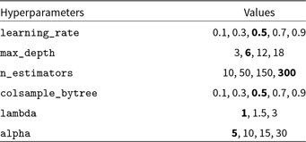
For training the XGBoost classifier with the similar input features used in Scalzo et al. (Reference Scalzo2017), we split the sample into training and testing sets of 43 593 and 71 307 candidates, respectively. One issue is that our binary classification does not have a balanced number of instances in the training set. This requires the use of a stratified sampling strategy to learn the features of each class equally. Next, the classifier has a list of hyperparameters that require fine-tuning in order to derive the best-possible model. We select test values of hyperparameters from a set of points in a coarse grid (see Table 1). We focused on hyperparameters that tend to have a high impact on the classification, such as control overfitting, learning rate, and complexity of the trees. Briefly the parameters are:
-
• learning_rate: step size shrinkage used in update to prevent over-fitting,
-
• max_depth: maximum depth of a tree,
-
• n_estimators: the number of trees in our ensemble,
-
• colsample_bytree: the subsample ratio of columns when constructing each tree,
-
• lambda: L2 regularisation term on weights,
-
• alpha: L1 regularisation term on weights.
The final parameters were chosen as the model with the lowest classification error, i.e. with both high completeness and high purity (see bold figures in Table 1).
3.2. Validation sample
To enable an accurate and unbiased assessment of classifier purity (Section 3.3), we need to define a ‘validation sample’—a random sample of objects with the weight factors based on the observed magnitude and RB scores. In the general case of an unweighted random sample, high RB scores are less common than low ones. Also, it is required to keep reasonable statistics for the rare, bright objects. We note that the distribution of classes in the validation set is unbalanced and neither reflects those in the training set perfectly nor those expected during the real transient search. The role of the validation set is to lead the parameters of the classifier towards best performance on real data. Hence, the distribution of classes in the validation set should ideally reflect that of the classes in the test set, so that the performance metrics will be similar on both sets. In other words, the validation set should reflect the expected data imbalance. The imbalance in our validation set thus leads to suboptimal performance. In Section 4 we test its performance in a real transient search during the O3 run.
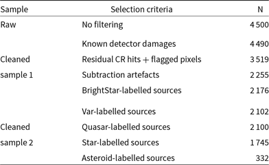
From a set of 149 DR3 i-band images, we obtained 11 790 sources with RBscore larger than 30 without any further filtering, and we selected 4 500 candidates for further visual inspection in a manner that sampled the range of source parameters. We label the sources irrespective of whether they have an automatic label or not. Table 2 summarises the steps we used to select pure transient candidates by removing known image artefacts (cleaned sample 1) and preselected categories (cleaned sample 2). Sample 1 can evaluate basic system performance, while sample 2 represents transient candidates that remain unexplained after automatic association with a known variable source and need to be presented for human vetting when hunting for real kilonovae.
Table 2. Sample selection criteria for purity test
Our main interest is in classifying either isolated (with no apparent host galaxy) or supernova-like transients with high completeness. To measure the classifier completeness (see Section 3.4), we initially used a total of 5 194 asteroid detections that were identified by SkyBot and 443 detections for 26 supernovae (16 SN Ia, 7 SN II, 1 SN IIn, 1 SN Ibc, and 1 SN Ic) that had been followed-up or discovered by the SkyMapper Transient Survey (Scalzo et al. Reference Scalzo2017; Möller et al. 2019).
We additionally use the Open Supernova Catalogue (Guillochon et al. Reference Guillochon, Parrent, Kelley and Margutti2017) to collect spectroscopically confirmed SNe with distances less than 250 Mpc. In order to match known SNe against DR3, we take a broad date range of
 $\pm30 \mathrm{d}$
from the SN discovery date as our reference epoch. With this selection cut, there are 429 i-band images of 318 SNe, where the position and epoch were matched with sources in the SMSS DR3 catalogue within 5 arcsec. Some of those DR3 sources are the host galaxies of SNe, or otherwise chance superpositions of unrelated sources. After running the image set through the AlertSDP pipeline, we recover 153 detections for 117 SNe which lie in the magnitude range between 15.5 and 20.5 in i band. Since the SMSS is focused on covering the entirety of the Southern Sky rather than frequently repeating a given area, most of the SNe only appear in a single exposure. By type, this sample contains 69 Type I SN (64 Ia, 2 Ib, 2 Ic, 1 Ib/Ic), 45 Type II SN (36 II, 4 IIP, 2 IIb, 3 IIn), and 3 unclassified ones, in a variety of host galaxies. Thus, our completeness test with the Open Supernova Catalog sample will be less affected by host galaxy selection effects than that of the SMT SNe sample. Figure 4 shows thumbnail images of representative SN examples in different redshift ranges. We assume that this validation sample contains a more representative sample of contaminants, but also represents the outcome of the pipeline more accurately than the training data used in the model development stage.
$\pm30 \mathrm{d}$
from the SN discovery date as our reference epoch. With this selection cut, there are 429 i-band images of 318 SNe, where the position and epoch were matched with sources in the SMSS DR3 catalogue within 5 arcsec. Some of those DR3 sources are the host galaxies of SNe, or otherwise chance superpositions of unrelated sources. After running the image set through the AlertSDP pipeline, we recover 153 detections for 117 SNe which lie in the magnitude range between 15.5 and 20.5 in i band. Since the SMSS is focused on covering the entirety of the Southern Sky rather than frequently repeating a given area, most of the SNe only appear in a single exposure. By type, this sample contains 69 Type I SN (64 Ia, 2 Ib, 2 Ic, 1 Ib/Ic), 45 Type II SN (36 II, 4 IIP, 2 IIb, 3 IIn), and 3 unclassified ones, in a variety of host galaxies. Thus, our completeness test with the Open Supernova Catalog sample will be less affected by host galaxy selection effects than that of the SMT SNe sample. Figure 4 shows thumbnail images of representative SN examples in different redshift ranges. We assume that this validation sample contains a more representative sample of contaminants, but also represents the outcome of the pipeline more accurately than the training data used in the model development stage.
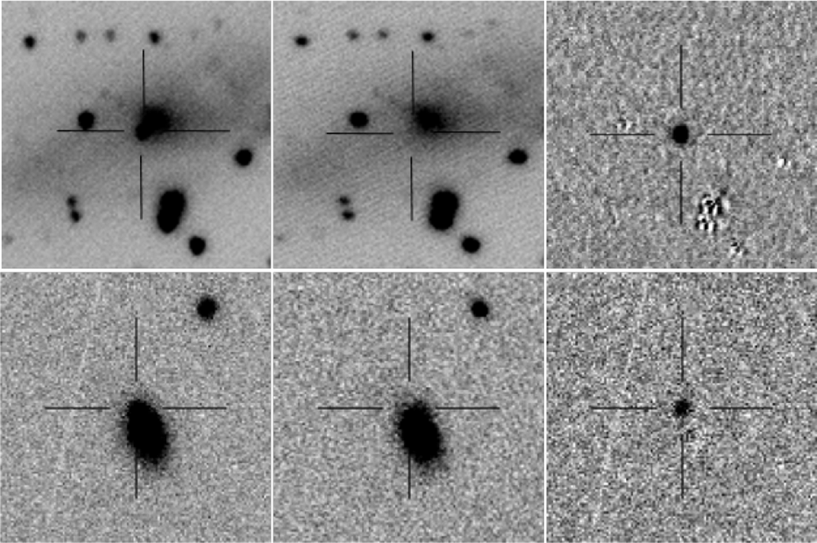
Figure 4. Thumbnail images of two supernovae in the SMSS DR3 i-band data set, showing the new, reference, and subtraction image from left to right (size:
 $1\, \textrm{arcmin} \times 1\, \textrm{arcmin}$
). Top: Type II SN 2019ejj at
$1\, \textrm{arcmin} \times 1\, \textrm{arcmin}$
). Top: Type II SN 2019ejj at
 $d=13\, \textrm{Mpc}$
, i = 17.1. Bottom: Type Ia-91T SN 2019ur at
$d=13\, \textrm{Mpc}$
, i = 17.1. Bottom: Type Ia-91T SN 2019ur at
 $d=250\, \textrm{Mpc}$
, i = 18.8.
$d=250\, \textrm{Mpc}$
, i = 18.8.
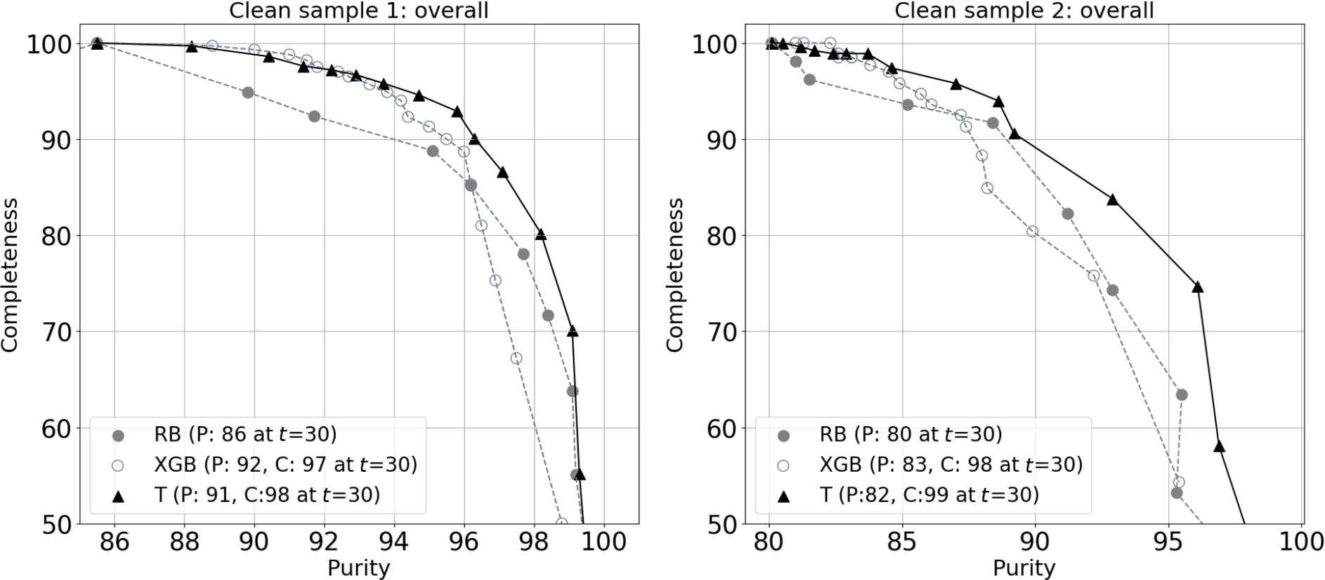
Figure 5. Purity vs completeness curves for the two cleaned samples described in Section 3.2. We compare the performance of three ensemble scores: RBscore (grey filled circle), XGBscore (grey open circle), and our new metric, Tscore (black filled triangle). The text in the panels refers to purity (P) and completeness (C) scores at a threshold of
 $t=30$
, which we adopt for our transient search.
$t=30$
, which we adopt for our transient search.
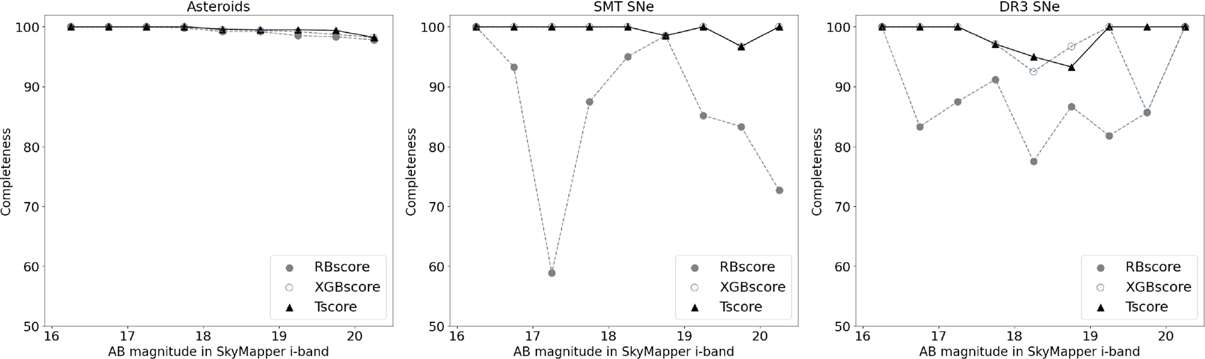
Figure 6. Completeness test with asteroid (left), SMT SN (middle), and DR3 SN (right) samples as a function of magnitude. We compare the three different ensemble scores: RBscore (grey filled circle), XGBscore (grey open circle), and Tscore (black filled triangle). The same axis ranges are used in each panel.
3.3. Purity test
As our two classifiers have different strengths, a combination of them can lead to better performance. XGBoost is much better at recognising bad subtractions with negative pixel values, whereas RF works better at recognising that CR hits and warm pixels are not real objects. While this may be the result of different training, we define a new metric here, Tscore, that combines the two machine learning models (known as an ensemble of classifiers; see Chapter 34 in Dietterich Reference Dietterich2000 for instance), using the simple rule:
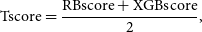 \[ {\rm{Tscore}} = \frac{\rm RBscore + \rm XGBscore}{2},\]
which gives both classifiers a similar weight.
For any threshold t, we define classifier purity:
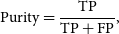 \[ \mathrm{Purity}= \frac{\rm TP}{\rm TP + \rm FP},\]
where TP is the number of true transients with any scores greater than t, and FP is the number of false positives that were incorrectly considered as real. Varying the threshold of a binary classifier usually trades off better completeness against better purity. In Figure 5, we show curves of completeness vs purity in our cleaned samples as a function of threshold and compare our two classifiers as well as the combined Tscore. In cleaned sample 1, XGBscore is an improvement over RBscore at every completeness
 $>90\%$
; for further applications, we choose a threshold of
$>90\%$
; for further applications, we choose a threshold of
 $t=30$
, which delivers 92% purity and 97% completeness. However, at higher purity the originally used RBscore appears more complete. Our new metric then combines the advantages of both and is in all parts of the curve at least as good as either the RB or XGB classifier. In cleaned sample 2 (right panel of Figure 5) all transient candidates explained by known objects have been removed and only those in need of human inspection are left over; here, a threshold of
$t=30$
, which delivers 92% purity and 97% completeness. However, at higher purity the originally used RBscore appears more complete. Our new metric then combines the advantages of both and is in all parts of the curve at least as good as either the RB or XGB classifier. In cleaned sample 2 (right panel of Figure 5) all transient candidates explained by known objects have been removed and only those in need of human inspection are left over; here, a threshold of
 $t=30$
is still a good choice and provides a purity above 80% with 99% completeness. Based on this, we choose the ensemble-based Tscore classifier with a threshold of
$t=30$
is still a good choice and provides a purity above 80% with 99% completeness. Based on this, we choose the ensemble-based Tscore classifier with a threshold of
 $t=30$
as our final classifier. Other wide-field surveys have obtained similar results on real-bogus classification by using convolutional neural networks (e.g. Duev et al. Reference Duev2019; Killestein et al. Reference Killestein2021).
$t=30$
as our final classifier. Other wide-field surveys have obtained similar results on real-bogus classification by using convolutional neural networks (e.g. Duev et al. Reference Duev2019; Killestein et al. Reference Killestein2021).
3.4. Completeness test
Next, we check the completeness of Tscore classifier for real-bogus classification. For any threshold t on the score, we obtain the completeness or recovery rate as a function of magnitude, using
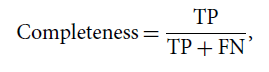 \[\mathrm{Completeness} = \frac{\rm TP}{\rm TP + FN},\]
where TP is the number of true positives in the test set that were correctly classified as real and FN is the number of false negatives (= positives misclassified as bogus). Figure 6 shows how the classifier performs as a function of magnitude for the two cases of asteroids and supernovae. In both cases, there is a clear trend for brighter transients to have a higher recovery rate at a given threshold. The high recovery rate of asteroids can be explained by the fact that they are over-represented in our training set compared to SN-like transients. Asteroids also appear mostly as isolated sources and are only rarely blended with galaxies, while supernovae and kilonovae are mostly blended with their host galaxy. With a threshold of
 $t=30$
, we attain 99.5% completeness for both asteroid (TP=55 170,170, FN=24) and supernova (TP=441, FN=2) classifications. While the SN sample has 443 detection images, these are from only 26 host galaxies and hence its statistical significance is smaller than it may seem. Moreover, there is reason to expect variations in completeness as a function of SN magnitude (at the time of detection), SN offset from the host galaxy nucleus, morphological type of the host galaxy, and redshift.
$t=30$
, we attain 99.5% completeness for both asteroid (TP=55 170,170, FN=24) and supernova (TP=441, FN=2) classifications. While the SN sample has 443 detection images, these are from only 26 host galaxies and hence its statistical significance is smaller than it may seem. Moreover, there is reason to expect variations in completeness as a function of SN magnitude (at the time of detection), SN offset from the host galaxy nucleus, morphological type of the host galaxy, and redshift.
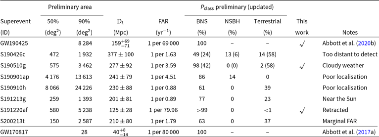
Table 3. Summary of preliminary BNS detection alerts in O3. For GW190425, we list updated information from Abbott et al. (Reference Abbott2020b)
To overcome this weakness, we test the completeness also for the DR3 SNe sample, which has fewer images but more (117 vs 26) host galaxies. Using
 $t=30$
again, we find high completeness (
$t=30$
again, we find high completeness (
 $\sim97\%$
; TP=148, FN=5) to the lowest magnitudes, comparable to other recently reported results (Killestein et al. Reference Killestein2021, with
$\sim97\%$
; TP=148, FN=5) to the lowest magnitudes, comparable to other recently reported results (Killestein et al. Reference Killestein2021, with
 $\sim $
97%). We checked the fives failures of the classifier and noticed that in three cases the FNs are superimposed on the host nucleus within
$\sim $
97%). We checked the fives failures of the classifier and noticed that in three cases the FNs are superimposed on the host nucleus within
 $<1$
arcsec offset, so that the classification may be affected by residual features from poor subtraction. The two SNe outside the nuclei of their hosts are OGLE 16etd, a classical SN II found close to maximum light in a crowded region, and SN 2018aau, an apparently hostless SN Ia detected
$<1$
arcsec offset, so that the classification may be affected by residual features from poor subtraction. The two SNe outside the nuclei of their hosts are OGLE 16etd, a classical SN II found close to maximum light in a crowded region, and SN 2018aau, an apparently hostless SN Ia detected
 $\sim 2$
weeks after maximum. The latter has two observations, one classified as TP and another one as FN. The classification scores of a given transient candidate can indeed vary with seeing conditions and star density in the field, which affect image subtraction.
$\sim 2$
weeks after maximum. The latter has two observations, one classified as TP and another one as FN. The classification scores of a given transient candidate can indeed vary with seeing conditions and star density in the field, which affect image subtraction.
4. Application in the LIGO/Virgo O3 run
Our follow-up programme was dedicated to the rapid search for kilonova counterparts to BNS mergers beyond GW170817 that would be observed by LIGO/Virgo observatories in O3. To trigger the SkyMapper observations, the estimated mass of one component of the compact binary system is required to be consistent with a neutron star (via the HasNS probability in the GCN notice). Table 3 summarises BNS candidates that have been reported in the LIGO/Virgo O3 public alerts, including events retracted later. For comparison, we list the properties of GW170817 detected in the O2 campaign in the last row of Table 3.
SkyMapper responded to three of these triggers, S190425z, S190510g and S191220af. The other triggers were ignored because of poor localisation or proximity to the Sun. The most promising event in all of O3 was S190425z, also called GW190425, where SkyMapper managed to obtain a data set of typical sky coverage. While we responded to the event in real time (see Section 4.1), we also reprocessed the data with the latest version of the AlertSDP to evaluate the real-world performance of the pipeline (see Section 4.2).
4.1. The search for an EM counterpart to S190425z/GW190425
On 2019 April 25 08:18:05.017 (UT), the LIGO Livingston observatory alone identified a GW chirp signal with a false alarm rate of one per 69 000 yr and a signal-to-noise ratio (SNR) of 12.9 (Abbott et al. Reference Abbott2020b). The LIGO Hanford facility was offline when the event was detected and the Virgo facility did not contribute to its detection due to a low SNR=2.5. This signal has strong evidence for the mass of one or both components to be consistent with a neutron star (
 $\mathrm{HasNS}= 100\%$
;
$\mathrm{HasNS}= 100\%$
;
 $\mathrm{BNS}=100\%$
). It also shows a clear time–frequency map with the characteristic upwardly sweeping chirp pattern expected for an inspiralling BNS system, which is what had been seen in GW170817 (see Figure 1 of Abbott et al. Reference Abbott2017a). The latest inferred position of this event was poorly localised in the sky, with a 90% credible sky area covering
$\mathrm{BNS}=100\%$
). It also shows a clear time–frequency map with the characteristic upwardly sweeping chirp pattern expected for an inspiralling BNS system, which is what had been seen in GW170817 (see Figure 1 of Abbott et al. Reference Abbott2017a). The latest inferred position of this event was poorly localised in the sky, with a 90% credible sky area covering
 $8\,284\, \mathrm{deg}^{2}$
, but the distance inferred from the GW signal was
$8\,284\, \mathrm{deg}^{2}$
, but the distance inferred from the GW signal was
 $159^{+69}_{-71} \mathrm{Mpc}$
(see Abbott et al. Reference Abbott2020b for details). Unlike the case of GW170817, where the position constraints were
$159^{+69}_{-71} \mathrm{Mpc}$
(see Abbott et al. Reference Abbott2020b for details). Unlike the case of GW170817, where the position constraints were
 $\sim 250\times$
tighter, this situation makes it difficult to find faint EM counterparts quickly. While the extremely wide-field Zwicky Transient Facility (ZTF) did search
$\sim 250\times$
tighter, this situation makes it difficult to find faint EM counterparts quickly. While the extremely wide-field Zwicky Transient Facility (ZTF) did search
 $\sim 8\,000\, \mathrm{deg}^2$
and reported two potential candidates, they needed two nights of observing to cover the area (Coughlin et al. Reference Coughlin2019). Some searches even reached sufficient depth to detect GW170817-like kilonovae, although their areal coverage was incomplete (Hosseinzadeh et al. Reference Hosseinzadeh2019).
$\sim 8\,000\, \mathrm{deg}^2$
and reported two potential candidates, they needed two nights of observing to cover the area (Coughlin et al. Reference Coughlin2019). Some searches even reached sufficient depth to detect GW170817-like kilonovae, although their areal coverage was incomplete (Hosseinzadeh et al. Reference Hosseinzadeh2019).
The first optical detection by SkyMapper was made from the prioritised list of target fields that were observed about 6 h after the merger. We let the search mode (Section 2.2) run on a relatively small fraction of the southern localisation region (
 $\sim125$
square degrees), acknowledging a small probability of finding the associated EM counterpart, as the area covered only
$\sim125$
square degrees), acknowledging a small probability of finding the associated EM counterpart, as the area covered only
 $\sim1\%$
of the initial BAYESTAR map and
$\sim1\%$
of the initial BAYESTAR map and
 $\sim3\%$
of its integrated probability. We found two transient candidates that had two detections separated by about 10 min, but neither of them had visible host galaxies. After the discovery of two candidates by the Zwicky Transient Facility (ZTF) survey, we moved onto a new phase to help determine whether either transient might be related to the GW signal. In Section 4.2, we perform a simple experiment to test our new software implementation with the SkyMapper observations of the BNS merger GW190425.
$\sim3\%$
of its integrated probability. We found two transient candidates that had two detections separated by about 10 min, but neither of them had visible host galaxies. After the discovery of two candidates by the Zwicky Transient Facility (ZTF) survey, we moved onto a new phase to help determine whether either transient might be related to the GW signal. In Section 4.2, we perform a simple experiment to test our new software implementation with the SkyMapper observations of the BNS merger GW190425.
As part of our Target-of-Opportunity programme at the ANU 2.3m Telescope, we obtained a series of early spectra of the potential counterpart ZTF19aarykkb (Coughlin et al. Reference Coughlin2019). We used the WiFeS instrument (Dopita et al. Reference Dopita, Hart, McGregor, Oates, Bloxham and Jones2007), whose integral-field nature allows us to obtain spectra of both the transient and the host galaxy simultaneously. These could identify a kilonova from its spectral features being atypical for better known transient types (e.g. cataclysmic variable stars or supernovae) and would also provide constraints on the environment of the transient as a birth or merger place for the progenitor binary (e.g. Levan et al. Reference Levan2017). We obtained our first 850 s exposure starting at 2019 April 25 17:40:40 UT, followed by
 $5\times1\,200\,\mathrm{s}$
spectra, using the
$5\times1\,200\,\mathrm{s}$
spectra, using the
 $R\sim3\,000$
gratings, B3000+R3000, covering the wavelength range of 320–990 nm. The WiFeS spectra showed the bright ZTF candidate (r= 18.63 mag) having spectral features similar to those of a young Type II supernova (Chang et al. Reference Chang2019b).
$R\sim3\,000$
gratings, B3000+R3000, covering the wavelength range of 320–990 nm. The WiFeS spectra showed the bright ZTF candidate (r= 18.63 mag) having spectral features similar to those of a young Type II supernova (Chang et al. Reference Chang2019b).
A number of additional EM candidates were discovered by other facilities (e.g. Hosseinzadeh et al. Reference Hosseinzadeh2019). At the location (RA=17:02:19.2, Dec=-12:29:08.2) of the Swift UVOT candidate by Breeveld et al. (Reference Breeveld2019) we did not see any transient down to an
 $i=20$
at the two epochs: 2019 April 25 14:17:00 and 2019 April 25 14:25:53 UT (Chang et al. Reference Chang, Wolf, Onken, Luvaul and Scott2019c). Later work suggested the Swift detection was likley to be an ultraviolet flare on an M dwarf star (Lipunov et al. Reference Lipunov2019; Bloom et al. Reference Bloom, Zucker, Schlafly, Finkbeiner, Martinez-Palomera, Goldstein and Andreoni2019). As discussed by previous studies, M dwarf flares are the most common transient phenomenon that may confuse searches for kilonova candidates from GW events (e.g. van Roestel et al. Reference van Roestel2019; Chang et al. Reference Chang, Wolf and Onken2020).
$i=20$
at the two epochs: 2019 April 25 14:17:00 and 2019 April 25 14:25:53 UT (Chang et al. Reference Chang, Wolf, Onken, Luvaul and Scott2019c). Later work suggested the Swift detection was likley to be an ultraviolet flare on an M dwarf star (Lipunov et al. Reference Lipunov2019; Bloom et al. Reference Bloom, Zucker, Schlafly, Finkbeiner, Martinez-Palomera, Goldstein and Andreoni2019). As discussed by previous studies, M dwarf flares are the most common transient phenomenon that may confuse searches for kilonova candidates from GW events (e.g. van Roestel et al. Reference van Roestel2019; Chang et al. Reference Chang, Wolf and Onken2020).
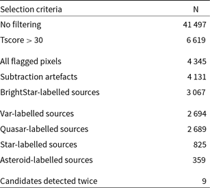
Table 4. Transient Selection for GW190425
4.2. SkyMapper search results for GW190425
To get a realistic view of the current performance of the SkyMapper transient facility, we reran the initial search mode data from the first night of the GW190425 event in O3 through the AlertSDP as described above. Each target field in the
 $\sim125$
square degrees of the localisation region was visited twice, separated by about 10 min. We applied the same filtering scheme for the selection of transient candidates as introduced in Section 3. Table 4 shows how each filtering step reduced the number of candidates from 41 497 to 359, which is a >100-fold reduction in the number of candidates requiring human inspection. Before the vetting process, this number was reduced even further to 9 candidates (1 in
$\sim125$
square degrees of the localisation region was visited twice, separated by about 10 min. We applied the same filtering scheme for the selection of transient candidates as introduced in Section 3. Table 4 shows how each filtering step reduced the number of candidates from 41 497 to 359, which is a >100-fold reduction in the number of candidates requiring human inspection. Before the vetting process, this number was reduced even further to 9 candidates (1 in
 $\sim5\,000$
) by considering only those with two detections. Each of the remaining candidates could be one of the following categories: (i) an isolated transient in a position which was not reported before, (ii) a galaxy with a SN at the time of observation, (iii) an as-yet unidentified variable object that has historical detections, or (iv) a bogus detection. We note that there was one known SN that was not detected in our search, because it was fainter than our detection limit (i = 20.4). Five of the sources were clear bogus detections caused by poor image subtraction. The remaining four candidates are persistent point sources in SMSS DR3 and seen to vary by 0.2–0.7 mag over the 5-year span of data in DR3. Thus, we conclude that none of them were related to GW190425.
$\sim5\,000$
) by considering only those with two detections. Each of the remaining candidates could be one of the following categories: (i) an isolated transient in a position which was not reported before, (ii) a galaxy with a SN at the time of observation, (iii) an as-yet unidentified variable object that has historical detections, or (iv) a bogus detection. We note that there was one known SN that was not detected in our search, because it was fainter than our detection limit (i = 20.4). Five of the sources were clear bogus detections caused by poor image subtraction. The remaining four candidates are persistent point sources in SMSS DR3 and seen to vary by 0.2–0.7 mag over the 5-year span of data in DR3. Thus, we conclude that none of them were related to GW190425.
5. Summary and outlook to O4
In this paper, we describe the capability of the SkyMapper facility for rapid-response EM observations of GW events. Developed as a new branch of the SkyMapper pipeline, the AlertSDP provides a prompt response to GW alerts with low-latency data processing and a web interface for follow-up. With a hybrid combination of ensemble-based classifiers, we achieve a high completeness (
 $\sim98\%$
) and purity (
$\sim98\%$
) and purity (
 $\sim91\%$
) in real-bogus classification; this is measured with a sample of 4 500 random transient candidates in the purity test, and over 5 000 asteroids as well as 143 supernovae in the completeness test. We performed the same analysis on the real SkyMapper data for LIGO/Virgo event S190425z/GW190425, confirming its efficiency to reduce contaminants.
$\sim91\%$
) in real-bogus classification; this is measured with a sample of 4 500 random transient candidates in the purity test, and over 5 000 asteroids as well as 143 supernovae in the completeness test. We performed the same analysis on the real SkyMapper data for LIGO/Virgo event S190425z/GW190425, confirming its efficiency to reduce contaminants.
When the observing run O4 starts with the GW detector network of the LIGO/Virgo/Kagra (LVK) collaboration, the predicted rate of BNS merger detections is
 $10^{+52}_{-10}$
per year, their predicted median luminosity distance is
$10^{+52}_{-10}$
per year, their predicted median luminosity distance is
 $170^{+6.3}_{-4.8} \mathrm{Mpc}$
, and their predicted median 90% sky localisation area is
$170^{+6.3}_{-4.8} \mathrm{Mpc}$
, and their predicted median 90% sky localisation area is
 $33^{+4.9}_{-5.3}\, \mathrm{deg}^{2}$
(all values given as 5%–95% confidence intervals; Abbott et al. Reference Abbott2020a). A 100-s i-band exposure with SkyMapper can discover an GW170817-like kilonova at four times the distance of GW170817. Future SMSS data releases will have deeper co-added reference images with up to 600 s exposures per sky pixel in each band, which may allow complete detection of transient candidates to
$33^{+4.9}_{-5.3}\, \mathrm{deg}^{2}$
(all values given as 5%–95% confidence intervals; Abbott et al. Reference Abbott2020a). A 100-s i-band exposure with SkyMapper can discover an GW170817-like kilonova at four times the distance of GW170817. Future SMSS data releases will have deeper co-added reference images with up to 600 s exposures per sky pixel in each band, which may allow complete detection of transient candidates to
 $i\approx 21$
mag and provide good coverage beyond the LVK median horizon of 170 Mpc. The AlertSDP should identify all transients in a
$i\approx 21$
mag and provide good coverage beyond the LVK median horizon of 170 Mpc. The AlertSDP should identify all transients in a
 $\sim 100\mathrm{deg}^{2}$
search area within 4 h from the start of observations. In the future, we expect to reduce this latency by speeding up the data processing.
$\sim 100\mathrm{deg}^{2}$
search area within 4 h from the start of observations. In the future, we expect to reduce this latency by speeding up the data processing.
Acknowledgements
We are grateful to an anonymous referee for comments that significantly improved the manuscript. We thank Jon Nielsen (ANU) for parallelising part of the AlertSDP. This research was partly funded by the Australian Research Council Centre of Excellence for Gravitational Wave Discovery (OzGrav), CE170100004. SWC acknowledges support from the National Research Foundation of Korea (NRF) grant, No. 2020R1A2C3011091, funded by the Korea government (MSIT). CAO acknowledges support from the Australian Research Council through Discovery Project DP190100252. The national facility capability for SkyMapper has been funded through ARC LIEF grant LE130100104 from the Australian Research Council, awarded to the University of Sydney, the Australian National University, Swinburne University of Technology, the University of Queensland, the University of Western Australia, the University of Melbourne, Curtin University of Technology, Monash University, and the Australian Astronomical Observatory. SkyMapper is owned and operated by The Australian National University’s Research School of Astronomy and Astrophysics. The survey data were processed and provided by the SkyMapper Team at ANU. The SkyMapper node of the All-Sky Virtual Observatory (ASVO) is hosted at the National Computational Infrastructure (NCI). Development and support of the SkyMapper node of the ASVO has been funded in part by Astronomy Australia Limited (AAL) and the Australian Government through the Commonwealth’s Education Investment Fund (EIF) and National Collaborative Research Infrastructure Strategy (NCRIS), particularly the National eResearch Collaboration Tools and Resources (NeCTAR) and the Australian National Data Service Projects (ANDS).


