2.1 Study area

The study site is located within a ∼ 1 km × 1 km area (Fig. 1a) in the Rur catchment near Selhausen (Germany; 50^∘51^′56^′′ N 6^∘27^′03^′′ E). It is composed of several agricultural fields cultivated in rotation by more than 20 different land owners, and thus the agricultural management is heterogeneous. The mean annual temperature and precipitation are 10.2 ^∘C and 715 mm, respectively (Rudolph et al., 2015). The area is part of the Terrestrial Environmental Observatories (TERENO) network (Bogena et al., 2018; Schmidt et al., 2012; Simmer et al., 2015). Within this network, continuous measurements of meteorological parameters are performed in the centre of field F11 (Fig. 1a).

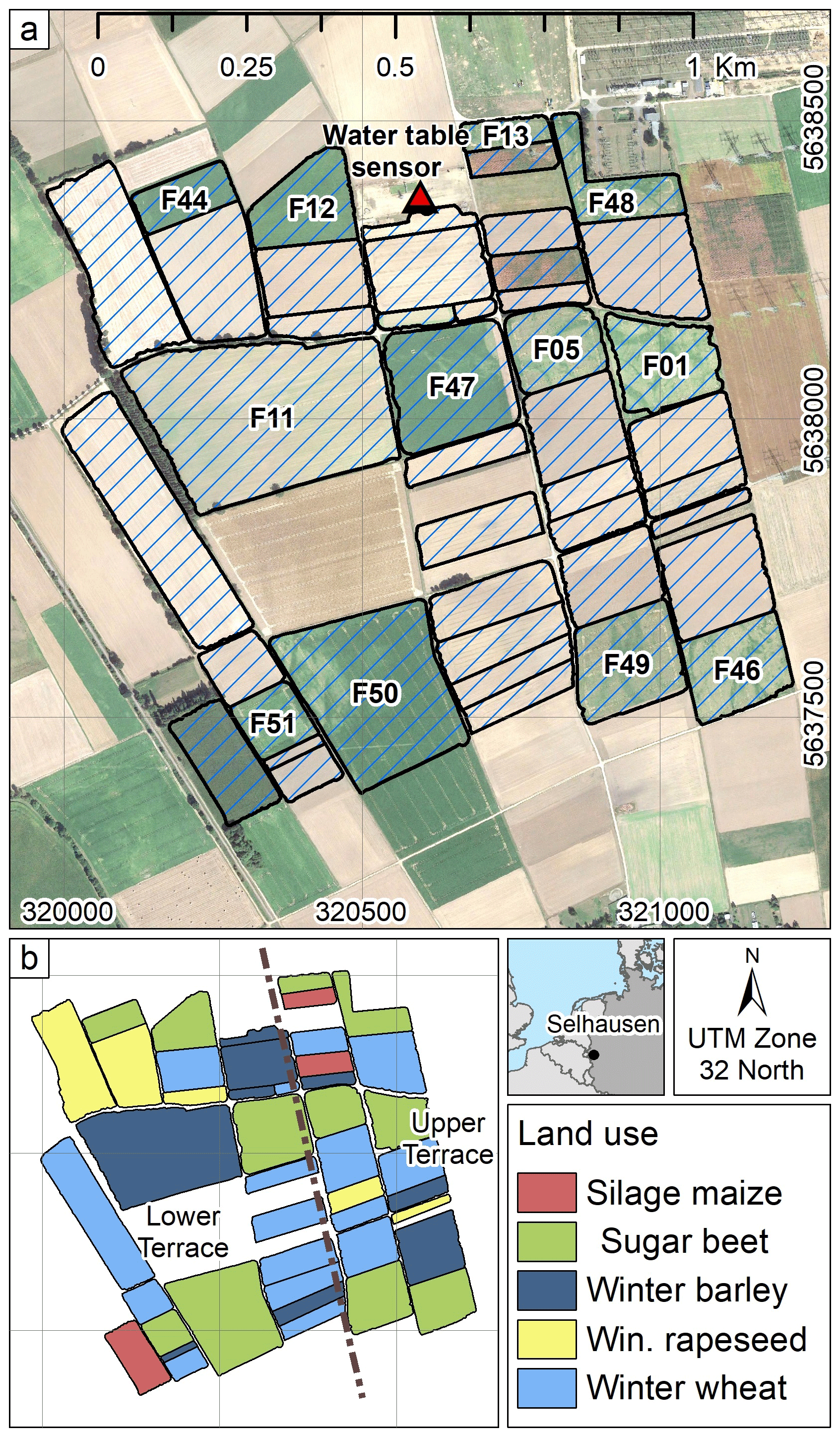
Figure 1(a) Satellite image of the study area with the fields used for comparison and codes of fields where sugar beet was grown in 2016 and (b) crops that were grown in each studied field in 2016 (ESRI, 2016).

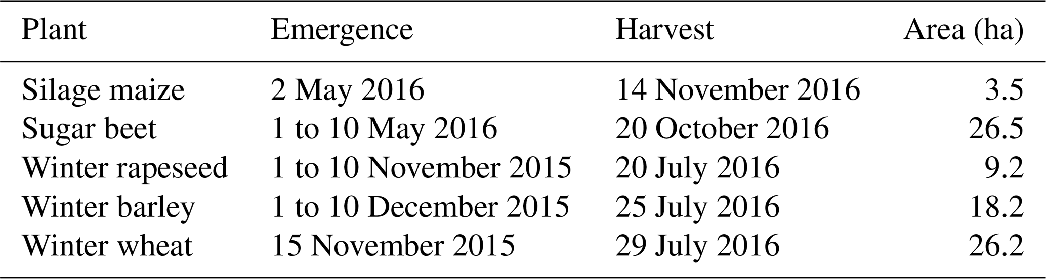
In 2016, the 44 investigated fields were cropped with silage maize, sugar beet, winter barley, winter rapeseed, and winter wheat. The distribution of these crops in the study area is shown in Fig. 1b. The total area cultivated with each crop, as well as their approximate emergence and harvest date, is listed in Table 1. A more detailed investigation was performed in fields where sugar beet was grown (fields F01, F05, F13a, F46, F48, F49, F12, F47, F50, and F51 in Fig. 1a). For field F01, the sugar beet yield for 2016 was 61.4 t ha⁻¹ of fresh beet, which is equal to 14.2 t ha⁻¹ of dry beet assuming an average water content of 76.8 % (FAO, 1999).

Table 1Range of emergence and harvest dates and total area for the five crops cultivated in the study area in 2016.

Download Print Version | Download XLSX

Previous studies at this site showed that soil heterogeneity has a strong influence on crop performance during long periods of water scarcity (Rudolph et al., 2015; von Hebel et al., 2018). This is most apparent on the upper terrace, which has an altitude of ∼ 110–113 m a.s.l. and is separated from the lower terrace (∼ 101–103 m a.s.l.) by a gentle slope with western exposition (Fig. 1). For both terraces, aeolian Pleistocene sediments and translocated Holocene loess (Röhrig, 1996) are generally dominant in the topsoil. Within the top 2 m of soil, sand and gravels from the Pleistocene and Holocene are consistently found below the aeolian sediments of the upper terrace and locally below the topsoils of the lower terrace (Brogi et al., 2019; Klostermann, 1992; Pätzold et al., 2008; Röhrig, 1996). The depth to these sand and gravels is known to be a strong control on crop water availability (Brogi et al., 2020; Rudolph et al., 2015; von Hebel et al., 2018).

Information on the spatial and temporal development of the five crops in 2016 was derived from multispectral satellite images. In particular, six LAI maps estimated from Level 3A images recorded by the RapidEye satellite constellation were available. These images covered the growing season of the five investigated crops and were acquired on 14 March, 20 April, 28 May, 9 June, 12 August, and 8 September 2016. In order to generate the LAI maps, the normalized difference vegetation index (NDVI) of the satellite images was first calculated using the red (RED; 630–685 nm) and the near-infrared (NIR; 760–850 nm) bands. In a second step, NDVI values were used to calculate the fractional vegetation cover (FVC_NDVI) for each image using the NDVI of bare soil (NDVI_S) and the fully vegetated state (NDVI_V) (Beck et al., 2006; Xiao and Moody, 2005; Zeng et al., 2003). Finally, the LAI_NDVI was calculated from the FVC_NDVI. In this final stage, the light extinction coefficient k(θ) of each crop type, which is a measure of attenuation of radiation in the canopy (Campbell, 1986; Norman and Campbell, 1989; Ross, 2012; Propastin and Erasmi, 2010), was calibrated using 45 in situ destructive LAI measurements that were acquired between 22 March and 7 September 2016. In the case of winter rapeseed and silage maize, no in situ LAI measurements were available, and k(θ) was obtained from literature values (Ali et al., 2015). A detailed description of the procedure used for this study area can be found in Brogi et al. (2020), whereas the general approach is described in more detail in Ali et al. (2015).

2.2 Available soil maps

Three different soil maps of the same area were used to inform agro-ecosystem simulations. Simulations were first performed using information from a geophysics-based soil map (Brogi et al., 2019) employing a methodology that was already successfully applied in this area by Brogi et al. (2020). In a following step, simulations were performed using information derived from two commonly available soil maps: (i) a regional soil map (Röhrig, 1996) with a scale of 1 : 5000 and (ii) a national soil and yield potential map (NRW, 1960) used in agricultural taxation.

The geophysics-based soil map (Fig. 2a) is a high-resolution product that was obtained by combining multi-configuration EMI measurements and direct soil sampling with subsequent laboratory analysis (Brogi et al., 2019). EMI measurements were performed using a CMD Mini Explorer – Special Edition (GF Instruments, Brno, Czech Republic) and resulted in six apparent electrical conductivity (ECa) maps, each with a different depth of investigation. These maps were analysed using a supervised classification methodology. This resulted in a map that showed the spatial distribution of 18 different soil types within the study area. Quantitative soil information was obtained using 100 augering locations (∼ one location per hectare) where horizon type and thickness were recorded. At these locations, soil samples were also collected to determine the grain size distribution of each soil horizon. Finally, information obtained through direct soil sampling was combined with the spatial distribution of the ECa-based soil units, which resulted in a soil map with 1 m resolution and quantitative soil information up to 2 m depth. The geophysics-based soil map consists of four sub-areas (A, B, C, and D) and a total of 18 soil units with an area between 0.6 and 16.0 ha. As shown in Fig. 2a for the soil units A1a and C1a, each soil unit of the geophysics-based soil map is provided with a soil profile that shows the depth of each horizon as well as the textural information (percentage of clay, silt, and sand plus gravels). A detailed description of the acquisition, management, and analysis of the geophysical data as well as the steps used to create this geophysics-based soil map can be found in Brogi et al. (2019). This geophysics-based product was recently used in several studies focused on the Selhausen study area (Brogi et al., 2020; Jakobi et al., 2020; Reichenau et al., 2020).

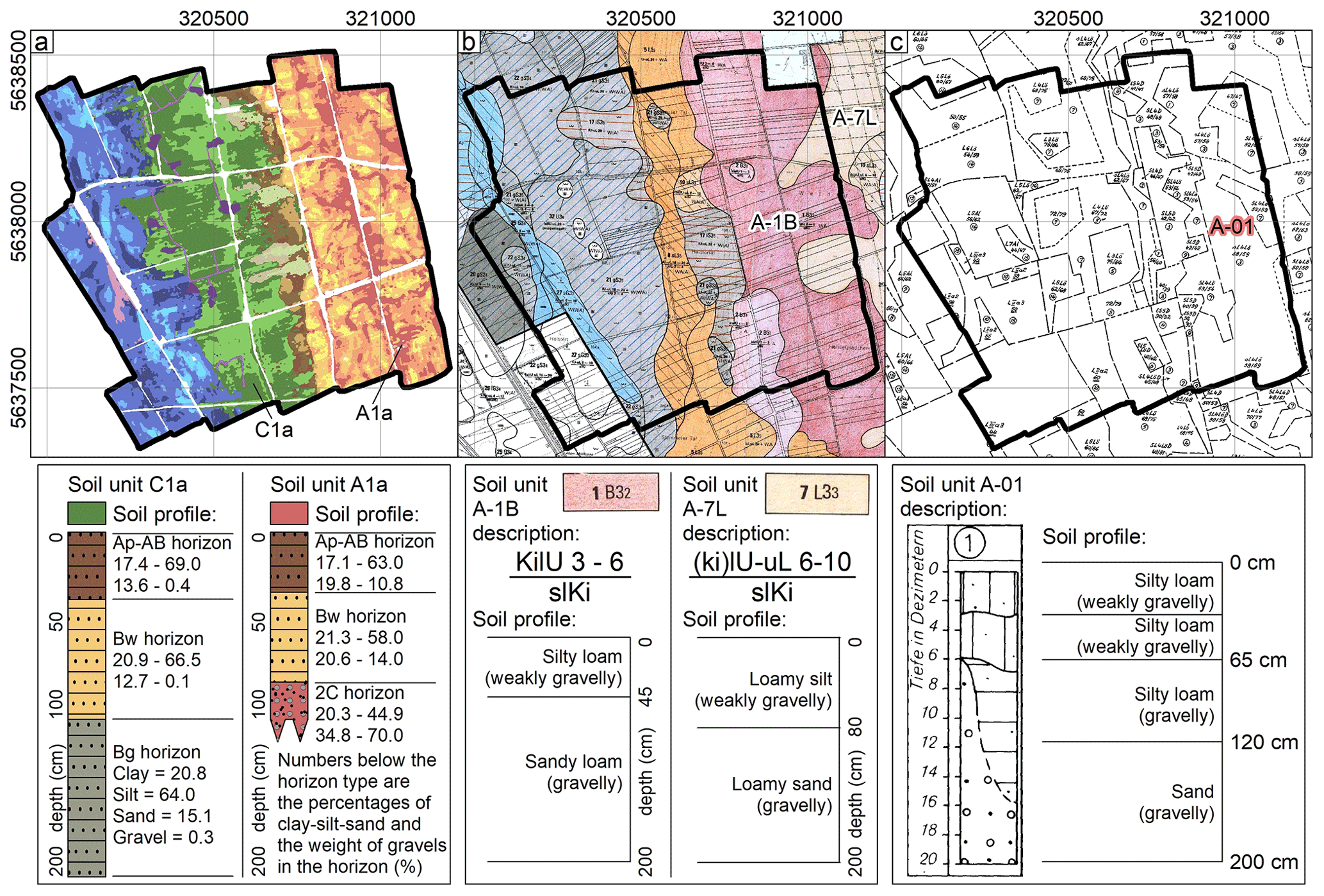
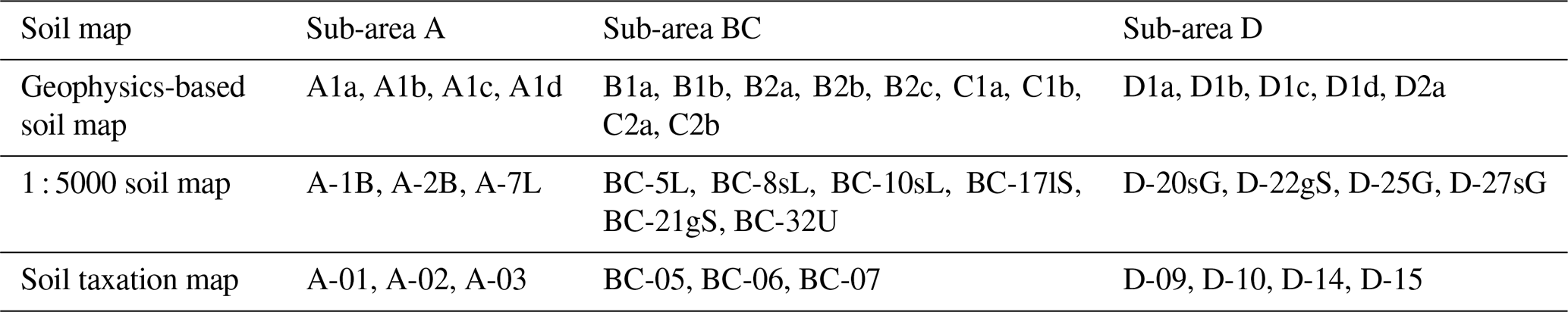
Figure 2(a) Geophysics-based soil map of the study area with examples of the quantitative description of the soil characteristics (soil units A1a and C1a are shown); (b) 1 : 5000 soil map of the study area with examples of the qualitative description of the soil characteristics (soil units A-1B and A-7L are shown) (Röhrig, 1996); and (c) soil taxation map of the study area and examples of the qualitative description of the soil characteristics (unit A-01 is shown) (NRW, 1960). The spatial distribution of all soil units within the study area and their codes are shown in Fig. 3.

The 1 : 5000 regional soil map is shown in Fig. 2b. This thematic map was first produced in 1984/85 and then revised in 1996 (Röhrig, 1996). It is commonly used in regional-scale projects (e.g. sustainable soil protection plans) and is part of the NRW official soil inventory (Geologischer Dienst NRW, 2018). The topographic base is the 1 : 5000 German base map (Deutsche Grundkarte), and soil information is obtained through direct soil sampling (augering). The distance between auger locations is typically <100 m (∼ one location per hectare). For each soil unit, information on soil type, soil texture (qualitative description), and thickness of the topsoil horizons is provided. Generally, the depth of the interface between two soil horizons is represented by a range (e.g. in soil unit A-1B of Fig. 2b, this interface is found between 0.3 and 0.6 m depth). This information was generalized by averaging the reported maximum and minimum values. According to this map, 13 soil units are found in the study area, with an area between 1.0 and 25.3 ha.

The soil taxation map is shown in Fig. 2c. It is used for the calculation of tax rates for farmers and land owners based on estimates of the yield potential (NRW, 1960). The scale of this map can vary across different regions in Germany and is 1 : 5000 for the study area. The map is based on the German cadastre, and soil information was obtained through direct soil sampling with a separation of 40 to 50 m between augering locations (∼ four locations per hectare). Each soil unit is described by a soil profile with 2.0 m depth, which is divided into up to four horizons. Each horizon carries qualitative information on soil texture. In some cases, the interface between two horizons is represented by a range, which again was generalized by averaging the reported maximum and minimum values (e.g. soil unit A-01 in Fig. 2c). In total, 10 different soil units were identified in the study area, and their area ranges between 0.7 and 17.5 ha.

The area covered by the five investigated crops in 2016 (Fig. 1b) and the geometry of the three soil maps (Fig. 3) were intersected. As a result, a set of unique soil–crop combinations was obtained for each soil map: (i) 72 unique soil–crop combinations for the geophysics-based soil map, (ii) 42 for the 1 : 5000 soil map, and (iii) 35 for the soil taxation map.

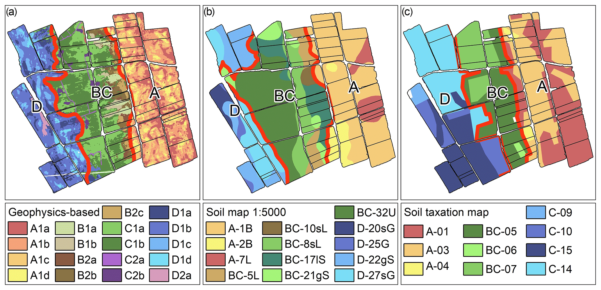
Figure 3Spatial distribution of soil units and of sub-areas A, BC, and D in (a) the geophysics-based soil map, (b) the 1 : 5000 soil map, and (c) the soil taxation map.

2.3 Similarities between sub-areas of the three soil maps

According to the geophysics-based soil map, the study area is divided into four sub-areas (A, B, C, and D) as described in Brogi et al. (2019). Sub-area A is located on the upper terrace, sub-area B is located on the slope between the two terraces, and sub-areas C and D are located on the lower terrace. Crop growth simulations for sub-areas B and C by Brogi et al. (2020) showed similar results. Thus, they were described together as a single sub-area BC in this study (Fig. 3). Generally, the geometry of the soil units described in the commonly available soil maps falls within one of the four sub-areas of the geophysics-based product. Thus, the soil units of the commonly available maps were matched with one of the sub-areas A, BC, and D. As a result, a clearer comparison between the simulations and the results obtained with different maps was possible. The distribution of the soil units described in the three soil maps is shown in Fig. 3, and the final unified code of each soil unit is provided in Table 2.

Table 2Unified codes of the soil units for the three soil maps.

Download Print Version | Download XLSX

2.4 The AgroC model

The AgroC model (Herbst et al., 2008) was used to simulate crop growth within each of the soil–crop combinations. In particular, we were interested in investigating how differences in soil water content dynamics and water availability as a consequence of differences in soil layering and soil hydraulic parameters affected crop growth. The agro-ecosystem model AgroC couples three main modules: SOILCO2, SUCROS, and RothC. SOILCO2 simulates vertical fluxes of water, heat, and CO₂ for a 1D soil column (Šimůnek et al., 1996; Šimůnek and Suarez, 1993); SUCROS simulates crop growth (Spitters et al., 1989); and RothC simulates organic carbon turnover (Coleman and Jenkinson, 2008).

In the SOILCO2 module, water flow in a given soil profile is described by the 1D Richards equation:

where θ (cm³ cm⁻³) is the volumetric water content, t is time, z is the vertical coordinate (cm), K(h) (cm h⁻¹) is the hydraulic conductivity as a function of pressure head h (cm), and Q (cm³ cm⁻³ h⁻¹) is the source–sink term accounting for root water uptake by crops. The hydraulic conductivity K and the volumetric water content θ as a function of pressure head are described by the Mualem–van Genuchten model:

and

where K_s is the saturated hydraulic conductivity (cm h⁻¹), m is a parameter that is set equal to $\mathrm{1}-\mathrm{1}/n$, θ_s and θ_r (cm³ cm⁻³) are the saturated and residual water content, respectively, α is a parameter corresponding approximately to the inverse of the air entry pressure (cm⁻¹), n (dimensionless) is a parameter related to the pore size distribution (Van Genuchten, 1980), and S_e is the dimensionless relative saturation defined as

The water demand is calculated in the SUCROS module. For a crop growing under optimal conditions, the potential evapotranspiration is divided between potential transpiration T_p (cm h⁻¹) and potential soil evaporation E_p (cm h⁻¹). Then, the potential root water uptake S_p (cm³ cm⁻³ h⁻¹) is calculated using

where β is the depth-dependent root distribution function. Afterwards, the depth-specific actual root water uptake Q is obtained from the potential root water uptake S_p using

where the water uptake is scaled by a water uptake stress factor φ that is dependent on the pressure head. The φ(h) factor is calculated using the Feddes et al. (1978) approach:

where h_0–3 (cm) are threshold pressure heads obtained from literature. These thresholds were set to h₀=0 cm, $h_{\mathrm{1}}=-\mathrm{20}$ cm, $h_{\mathrm{2}}=-\mathrm{5000}$ cm, and h₃ = −16 000 cm (Vanclooster et al., 1995). The actual root water uptake is integrated over the rooting depth to obtain the actual transpiration. Afterwards, the ratio between actual and potential transpiration is used to simulate carbon assimilation and biomass production, which are also affected by additional variables such as temperature and solar radiation. A detailed description of this model and of the effects of simulated water stress on simulated crop growth can be found in Klosterhalfen et al. (2017) and in Brogi et al. (2020) for this study area.

2.5 Estimation of soil hydraulic parameters

Soil hydraulic parameters for each horizon of the soil units of all three soil maps were estimated from texture and bulk density using pedotransfer functions (PTFs) and a correction for gravel content as successfully done by Brogi et al. (2020) for the same area. Information on bulk density was not available. Therefore, the bulk density of the fine fraction <2 mm, BD_<2, of each horizon was assumed to be 1.30 g cm⁻³ for the Ap horizon, 1.40 g cm⁻³ for the AB horizon, 1.50 g cm⁻³ for deeper horizons with fine sediments, and 1.60 g cm⁻³ for deeper horizons with coarse sediments. These estimates were based on literature values and on results from previous sampling campaigns conducted within the study area (Brogi et al., 2020; Ehlers et al., 1983; Unger and Jones, 1998). Unfortunately, the soil profiles from the 1 : 5000 soil map and from the soil taxation map are not provided with the depth of the interface between the Ap and AB. Therefore, in each soil profile, the first horizon was subdivided at a depth of 0.3 m as this was generally observed to be the depth of the Ap horizon in this study area.

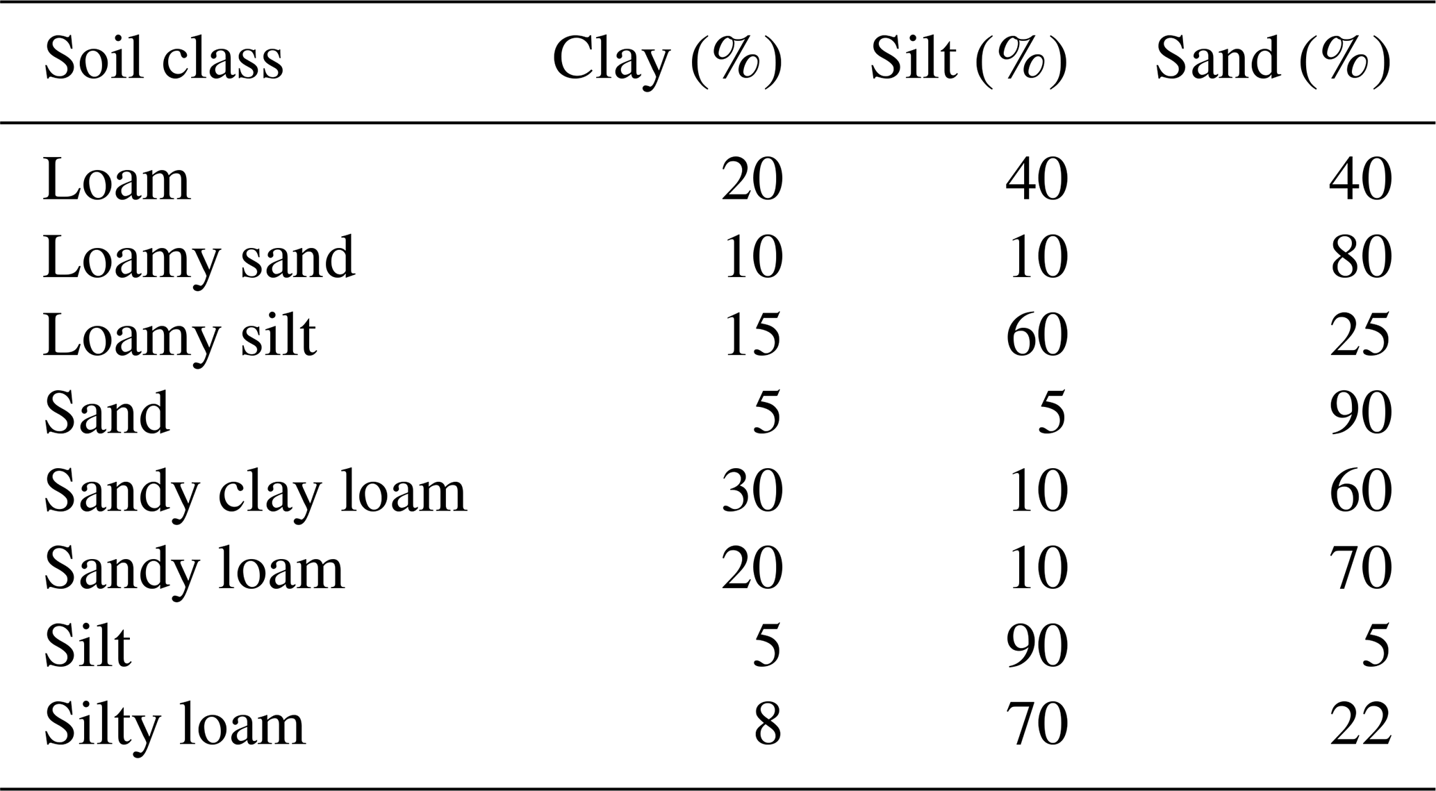
The geophysics-based soil map provides quantitative information on soil texture for each soil unit. In this case, the percentages of clay, silt, and sand were directly used in the estimation of the soil hydraulic parameters. In contrast, the two commonly available soil maps provide a qualitative description of soil texture (i.e. a soil textural class). Generally, lookup tables are used in the case of such qualitative descriptions (Van Looy et al., 2017) in order to obtain class-average soil hydraulic parameters (Baker, 1978; Bouma, 1989). To obtain a consistent comparison between the three maps, these qualitative soil textural class descriptions were translated into quantitative percentages of sand, silt, and clay using the USDA soil textural classification (USDA, 2019). For this, the centroid of each soil textural class within the USDA triangle was calculated to determine the associated soil texture percentages (Table 3). In some cases, the presence of gravel was qualitatively described in the two commonly available soil maps. In these cases, a 25 % volume of gravel was assumed when the gravel content was defined as “gravelly” and 10 % was assumed when the gravel content was defined as “weakly gravelly” as these percentages matched those observed in the study area.

Table 3Percentage (%) of sand, silt, and clay of the centroid of relevant soil textural classes within the USDA soil texture triangle.

Download Print Version | Download XLSX

The dry bulk density was estimated for each soil horizon using the equation of Brakensiek and Rawls (1994):

where BD_t is the dry bulk density of the soil, BD_>2 is the dry bulk density of gravel material, and G_v is the volume of gravel calculated from the percentage of weight according to Flint and Childs (1984). Finally, the soil hydraulic parameters θ_s, θ_r, α, n, and K_s were estimated from the dry bulk density and from clay, silt, and sand percentages by using the PTFs of Rawls and Brakensiek (1985). In all the soil maps, the estimated K_s values of the coarse horizons in sub-areas A and D were corrected for gravel content using the correction from Brakensiek and Rawls (1994):

where K_b is the saturated hydraulic conductivity of the bulk soil, and K_s is obtained from the PTF of Rawls and Brakensiek (1985).

As shown in Brogi et al. (2020), the coarse horizon 2C (sand and gravel) that underlies the fine aeolian sediments in sub-area A and in parts of sub-area D is of primary importance for a sound simulation of crop performance within the investigated area. However, the properties of these deeper soil horizons were not adequately captured in the commonly available soil maps, and this resulted in simulated water contents that were unrealistically low. To avoid the introduction of such strong and unrealistic variations in the results of the agro-ecosystem simulations performed with the three soil maps, the soil hydraulic parameters obtained for the 2C horizon in sub-areas A and D of the geophysics-based soil map were integrated into the two other commonly available soil maps.

2.6 Setup and evaluation of AgroC simulations

The 1D soil column used in the AgroC simulations was discretized by using a maximum of 252 nodes with a spacing of 1 mm near the soil surface and a gradual increase with depth until a maximum of 10 mm. The simulation period extended from 1 July 2015 to 31 December 2016. The simulation domain of the soil units in sub-area BC extended to 2.0 m below the soil surface for all three soil maps. In these units, a variable pressure head with an annual sinusoidal variation based on water table depth observations in field F10 (Fig. 1) was used as the lower boundary condition. The groundwater table depth was set to a minimum of −2.0 m on 15 January and a maximum of −2.6 m on 15 July. The initial pressure head within the soil profile was defined through a spin-up simulation. To achieve this, the period from 1 January 2015 to 31 December 2016 was repeatedly run until no change in pressure head within the soil column was observed between consecutive model runs.

The soil units of sub-areas A and D have a coarse sand and gravel horizon at depth. In these soil units, the simulation domain extended 30 mm into the coarse horizon. As a result, the simulation domain varied in depth between 0.52 and 1.57 m for the geophysics-based soil map and from 0.33 to 1.43 m in the two commonly available soil maps. Free drainage was used as the lower boundary condition for these soil units. The initial pressure head of the lower coarse horizons was set to −10 mm, and hydrostatic equilibrium was assumed throughout the profile (Brogi et al., 2020).

The required crop-specific parameters were mostly obtained from various literature sources (Allen et al., 1998; Bolinder et al., 1997; Boons-Prins et al., 1993; Borg and Grimes, 1986; Penning de Vries et al., 1989; Spitters et al., 1989; Van Heemst, 1988; Vanclooster et al., 1995). Only the sub-area specific parameterization of the death rate of leaves for sugar beet, the start of the senescence stage for silage maize, and the partitioning of aboveground biomass for winter wheat were adapted as described in detail in Brogi et al. (2020). The crop-specific maximum rooting depth was set to 1.50 m for sugar beet and silage maize, 1.40 m for winter rapeseed, 1.20 m for winter barley, and 1.00 m for winter wheat. The method of Rum et al. (1974) was used to calculate the root distribution above these depths. In the case of the soil units of sub-areas A and D, rooting depth was reduced using the depth of the lower coarse horizon as it was assumed that roots cannot penetrate into such coarse soils (Daddow and Warrington, 1983).

Three criteria were used to quantify the agreement between the observed LAI_NDVI and LAI simulated with AgroC by using inputs from the three soil maps. The first was the root mean square error (RMSE):

where n represents the number of observations, Obs_i is the observed value, and Sim_i is the simulated value. A lower RMSE indicates a better fit. The second criterion was the model efficiency (ME), which is calculated as

where $\stackrel{\mathrm{‾}}{\mathrm{Obs}}$ is the observed mean. The ME can vary between −∞ and 1, and a value higher than 0 indicates that the model describes the data better than the mean. A ME value of 1 indicates perfect agreement between observations and predictions (Nash and Sutcliffe, 1970). The third and final criterion was the coefficient of determination R²:

where $\stackrel{\mathrm{‾}}{\mathrm{Sim}}$ is the simulated mean. The value of R² ranges between 0 and 1, and a value of 1 indicates perfect agreement.

3.1 Comparison of the spatial distribution of soil properties in the three maps

By visually comparing the three soil maps, it is apparent that the geomorphological border between the upper and lower terrace is similarly identified (division between sub-area A and BC in Fig. 3). In the geophysics-based soil map, this subdivision is based on the measured apparent electrical conductivity (ECa) data (Brogi et al., 2019), whereas the delineation in the commonly available soil maps was mainly based on coarse soil augering and topography since this limit approximately coincides with the top of the slope that divides these two sub-areas. The location of the subdivision between sub-areas BC and D showed stronger differences between the three maps. Again, this border is obtained from ECa data in the geophysics-based soil map. In this case, there is no topographic feature associated with this subdivision, and, in the other two maps, only the information from augering was available to determine its position. This likely explains why the subdivision between the two sub-areas locally coincides with field boundaries in the 1 : 5000 soil map and in the soil taxation map.

Figure 4Percentages of sand (orange colour scale) and silt (brown colour scale) at 0.30 m depth and at 1.50 m depth in the three soil maps.

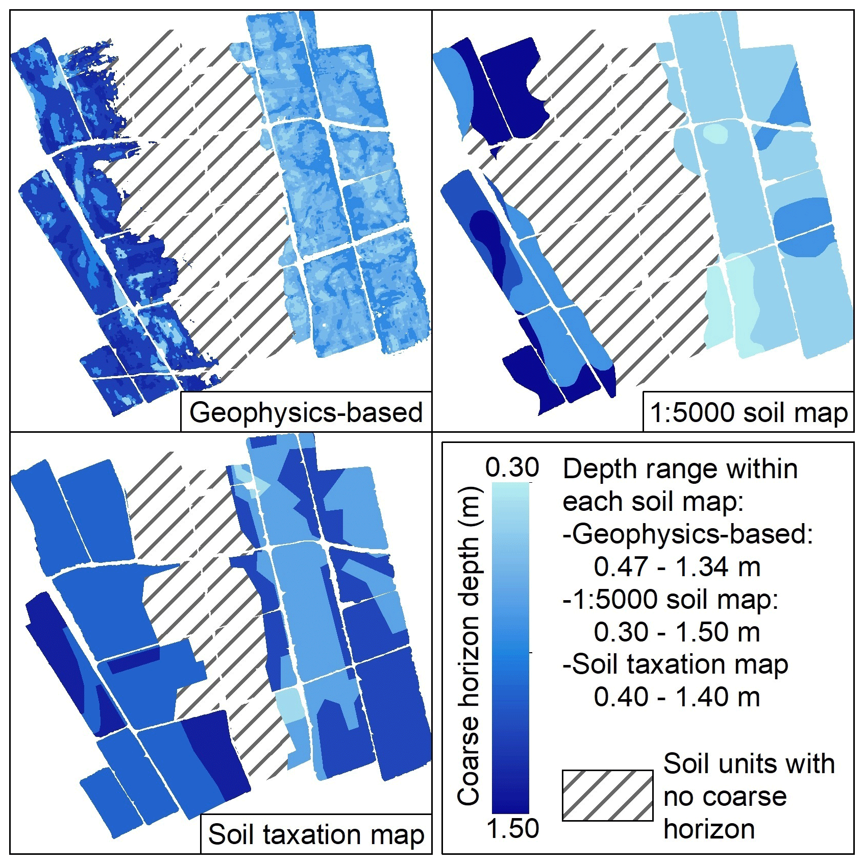
Figure 5Depth of the coarse horizon 2C in the three soil maps.

The geophysics-based soil map generally identifies a larger number of soil units with more complex polygon shapes compared to the commonly available soil maps. This is a consequence of the high resolution of the measured ECa data. In this study area, a single agricultural field contained four to nine soil units according to the geophysics-based soil map. The two commonly available soil maps often integrate larger areas into one soil unit, and a single field is composed of a maximum of four soil units. However, many fields contain only one soil unit.

In the 1 : 5000 soil map and in the soil taxation map, the shallow soils found within the study area are generally silty loam and loamy silt above coarse sediments. As shown in Fig. 4, the grain size distribution obtained from the qualitative descriptions using Table 3 showed minor differences compared to the one provided by the soil units of the geophysics-based soil. For example, the estimated grain size distribution for loamy silt soil units of the commonly available maps was 25 % sand, 60 % silt, and 15 % clay, whereas the respective range of values found in the geophysics-based soil map was 13 %–24 % sand, ∼ 56 %–70 % silt, and ∼ 13 %–23 % clay. The estimated values for silty loam (22 % sand, 70 % silt, and 8 % clay) differed more from those of the geophysics-based soil map but still were in reasonable agreement. The underlying coarse materials found in sub-areas A and D were identified as loamy sand, sand, sandy clay loam, or sandy loam in the commonly available soil maps. In the case of these four soil textural classes, the sand fraction reported in Table 3 (60 %–90 %) was much higher than the values reported in the geophysics-based soil map (∼ 28 %–58 %). At the same time, the percentage of silt in the commonly available maps (5 %–10 %) was much lower compared to those of the geophysics-based map (∼ 30 %–54 %). Figure 4 illustrates these textural differences in sand and silt percentages between the three soil maps at a depth of 1.50 m.

The description of the topsoil (at 0.3 m depth) in the three soil maps is rather similar. In contrast, the geophysics-based soil map provides a different description of the underlying coarse horizons compared to the commonly available soil maps. It is important to note that the textural compositions found in the geophysics-based soil map were determined from laboratory analysis, whereas those provided by the other two maps were generated from field estimations (hand texturing). Due to these differences, soil hydraulic parameters of the coarse sediments vary strongly between the three maps, with the commonly available maps showing much higher values of K_s and θ_s. As already mentioned in the Materials and methods section, this resulted in unrealistic simulations with very low soil water content for the commonly available maps (results not shown). For this reason, the soil hydraulic parameters of the coarse horizons of sub-areas A and D of the geophysics-based soil map were integrated into the simulations based on the two commonly available soil maps.

Differences in the depth to the coarse sand and gravel that underlie the fine sediments in sub-areas A and D were observed between the three soil maps (Fig. 5). In all three maps, this depth was obtained from augering information and varied between 0.47 and 1.34 m in the geophysics-based soil map, between 0.30 and 1.50 m in the 1 : 5000 soil map, and between 0.40 and 1.40 m in the soil taxation map. Both the two commonly available soil maps showed a larger depth range than that of the geophysics-based soil map, with the 1 : 5000 soil map showing the largest depth range.

3.2 Performance of LAI simulations

Figure 6 shows a comparison between the mean observed LAI_NDVI for each soil–crop combination and the LAI simulated with AgroC by using inputs from the three soil maps. The LAI simulations based on the geophysics-based soil map (R²=0.925, ME = 0.919, and RMSE = 0.604) were more able to describe LAI_NDVI compared to the simulations based on the 1 : 5000 soil map (R²=0.887, ME = 0.869, and RMSE = 0.718) and the soil taxation map (R²=0.886, ME = 0.866, and RMSE = 0.719). However, the results for all three soil maps could be considered satisfactory as the improvement provided by the more detailed geophysics-based soil map is relatively small. This similarity in model quality can be explained by the simultaneous use of all simulated crops (silage maize, sugar beet, winter barley, winter rapeseed, and winter wheat) and all six RapidEye satellite images. Furthermore, this comparison was performed by using the mean value for each soil–crop combination, and this reduced the influence of small-scale variability of LAI_NDVI. These aspects will be investigated in more detail in the next section.

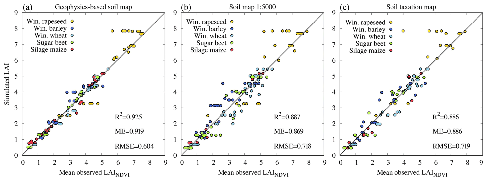
Figure 6Simulated LAI and mean observed LAI_NDVI for each soil–crop combination for simulations based on (a) the geophysics-based soil map, (b) the 1 : 5000 soil map, and (c) the soil taxation map for all six available RapidEye images.

Download

3.3 Pixel-by-pixel comparison of LAI simulations

Figure 7 shows a pixel-by-pixel comparison of observed LAI_NDVI and LAI simulated using inputs from the three soil maps. It is apparent how the highest pixel density (red) is close to the 1 : 1 line for the geophysics-based soil map, and more spread is observed for the two commonly available soil maps. Moreover, the error measures for the geophysics-based soil map (R²=0.884, ME = 0.878, and RMSE = 0.689) show slightly better results than those of the 1 : 5000 soil map (R²=0.858, ME = 0.847, and RMSE = 0.774) and considerably better results than those of the soil taxation map (R²=0.741, ME = 0.675, and RMSE = 1.126). The values of LAI_NDVI occasionally showed a rather strong variability within single soil–crop combinations. As a consequence, lower values of R² and ME and higher values of RMSE are found in the pixel-by-pixel analysis compared to the previously discussed comparison that made use of the mean LAI_NDVI for each soil–crop combination.

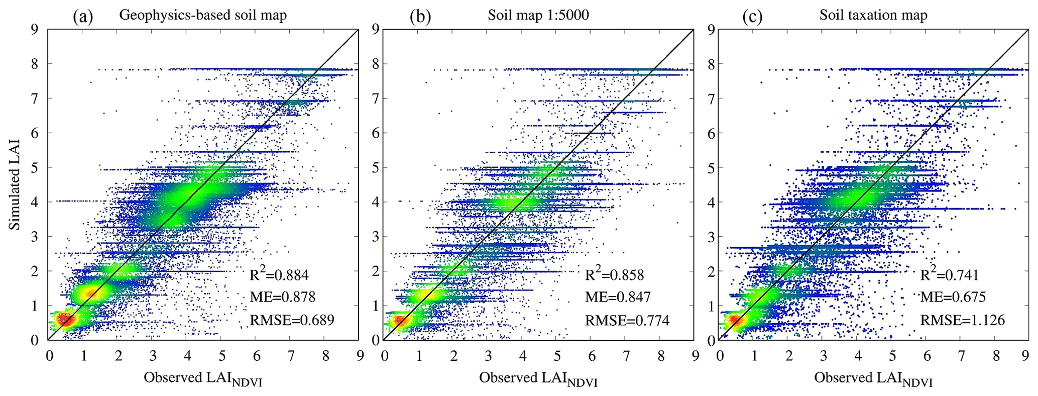
Figure 7Pixel-by-pixel comparison between simulated LAI and observed LAI_NDVI for simulations based on (a) the geophysics-based soil map, (b) the 1 : 5000 soil map, and (c) the soil taxation map. The colour indicates the density of events, with red representing the highest density and blue the lowest density.

Download

Table 4R², ME, and RMSE of the pixel-by-pixel comparison of the three soil maps performed between simulated LAI and observed LAI_NDVI of each soil–crop unit. The highest R² and ME and the lowest RMSE at each date are marked in bold.

Download Print Version | Download XLSX

Table 4 shows the pixel-by-pixel performance of the three soil maps for each RapidEye satellite image. The geophysics-based soil map generally showed higher ME and higher R² and lower RMSE. However, it is apparent that the three soil maps performed similarly in March, May, and June, when winter crops were grown (i.e. winter barley, winter rapeseed, and winter wheat), with the 1 : 5000 soil map showing marginally higher ME and R² for individual dates. Given the sufficient amount of rain during the growth of these crops, simulations showed little crop water stress. This resulted in simulations with rather similar LAI despite using information from three different soil maps. In the case of the image from April, the geophysics-based soil map and the 1 : 5000 soil map outperformed the soil taxation map. However, a general decrease in performance can be observed for all three maps. This general decrease is likely caused by the high variability in LAI_NDVI between different agricultural fields, which is caused by the uncertainty in seeding and emergence dates of winter crops. Moreover, the flowering of winter rapeseed (yellow dots in Fig. 6) affected the estimated LAI_NDVI (Brogi et al., 2020). This may have additionally reduced the performance for all three soil maps in April. A strong drop in performance for all three soil maps was observed in August and September. At this stage, the comparison is based solely on silage maize and sugar beet as the other crop types were already harvested. Thus, the reduced correlation is likely related to the appearance of stress in these two crops that increased the spatial variability in LAI_NDVI. In this situation of high water stress, the geophysics-based soil map clearly outperformed the 1 : 5000 soil map and the soil taxation map, especially towards the end of the growing season.

3.4 Simulation of sugar beet

In a next step, simulations of sugar beet are analysed in more detail because of the importance of this crop (sugar beet represents 31.7 % of the investigated area) and because the previously described analysis showed that the difference in performance between the three soil maps was the greatest when this crop was still growing (August and September). Figure 8a–c show the simulated LAI (lines) and the observed LAI_NDVI (dots) for sugar beet grown on the soil units of sub-area A for the three soil maps. Figure 8d–f show the associated water stress simulated with AgroC. All these simulations made use of the same crop parameterization. Thus, the differences in simulated LAI are due to different degrees of water stress associated with the soil characteristics. As shown in Fig. 8a, the simulated LAI based on the geophysics-based soil map matched well with the observations. In fact, soil units A1a-d showed very similar LAI values for 28 May and 9 June. Later in the growing season (12 August and 8 September), simulated LAI of soil units A1a-d differed due to a different magnitude of water stress. The magnitude of water stress and the consequent reduction of LAI are well correlated with the depth of the coarse sediments, which was 0.86 m in soil unit A1a, 0.67 m in A1b, 0.58 m in A1c, and 0.49 m in A1d.

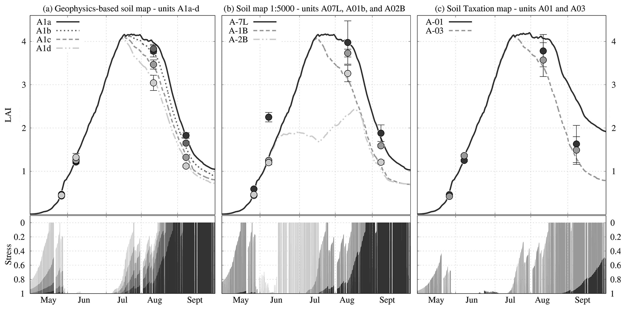
Figure 8Observed LAI_NDVI (dots) of sugar beet compared to the simulated LAI (lines) in sub-area A (upper plots) as well as corresponding stress occurrence (lower plots) simulated using input from (a) the geophysics-based soil map, (b) the 1 : 5000 soil map, and (c) the soil taxation map.

Download

In the case of the three soil units of the 1 : 5000 soil map, the simulated LAI matched well the observations in May and June, with the only exception of soil unit A-07L, where observed LAI_NDVI is underestimated. Later in the growing season (August and September), soil unit A-7L again matched the observations. This was not the case for soil units A-1B and A-2B, where LAI_NDVI was underestimated. The mismatch between LAI simulations and observations for these two soil units is due to the assumed shallow depth to the coarse sediments (0.30 m in soil unit A-2B, 0.45 m in unit A-1B, and 0.80 m in A-7L). As previously discussed, this depth has a strong influence on the intensity and timing of water stress. Generally, the topsoil and the associated physical properties described in the 1 : 5000 soil map were rather similar to those of the geophysics-based soil map. As a consequence, the reduced match between simulated LAI and observed LAI_NDVI was caused by an underestimation of the depth to the coarse sediments in soil units A-1B and A-2B, which resulted in a higher water stress and lower LAI.

In the case of the soil taxation map, the observed LAI_NDVI for the two soil units A-01 and A-03 were rather similar and showed a strong variability within each unit (see dots and error bars in Fig. 8c). This suggests that the geometry of the two soil units did not capture the spatial differences in crop performance present in the LAI_NDVI. The soil physical properties of the uppermost horizon in the soil taxation map were rather different compared to those of the geophysics-based soil map. In contrast, the soil physical properties of the coarse sediments were equal to those of the geophysics-based soil map by design. However, the depth to these coarse sediments in the two soil units was generally deeper (1.20 m in A-01 and 0.70 m in A-03) than in the geophysics-based soil map. Due to these different soil physical properties and the overestimation of soil depth overestimation, lower water stress in soil unit A-01 caused a higher simulated LAI compared to the observations. This depth was better captured in soil unit A-03 that showed better LAI simulations.

Figure 9 shows the spatial distribution of LAI_NDVI for 12 August and 8 September. On both days, the large-scale pattern in LAI_NDVI associated with the differences between sub-areas A, BC, and D was clearly visible. In August (Fig. 9a), LAI_NDVI reached the maximum observed value in sub-area BC, whereas lower values were observed in sub-area A due to water stress. In September (Fig. 9b), the development of sugar beet was affected by water stress in both sub-area A and D, as indicated by the lower LAI_NDVI compared to sub-area BC.

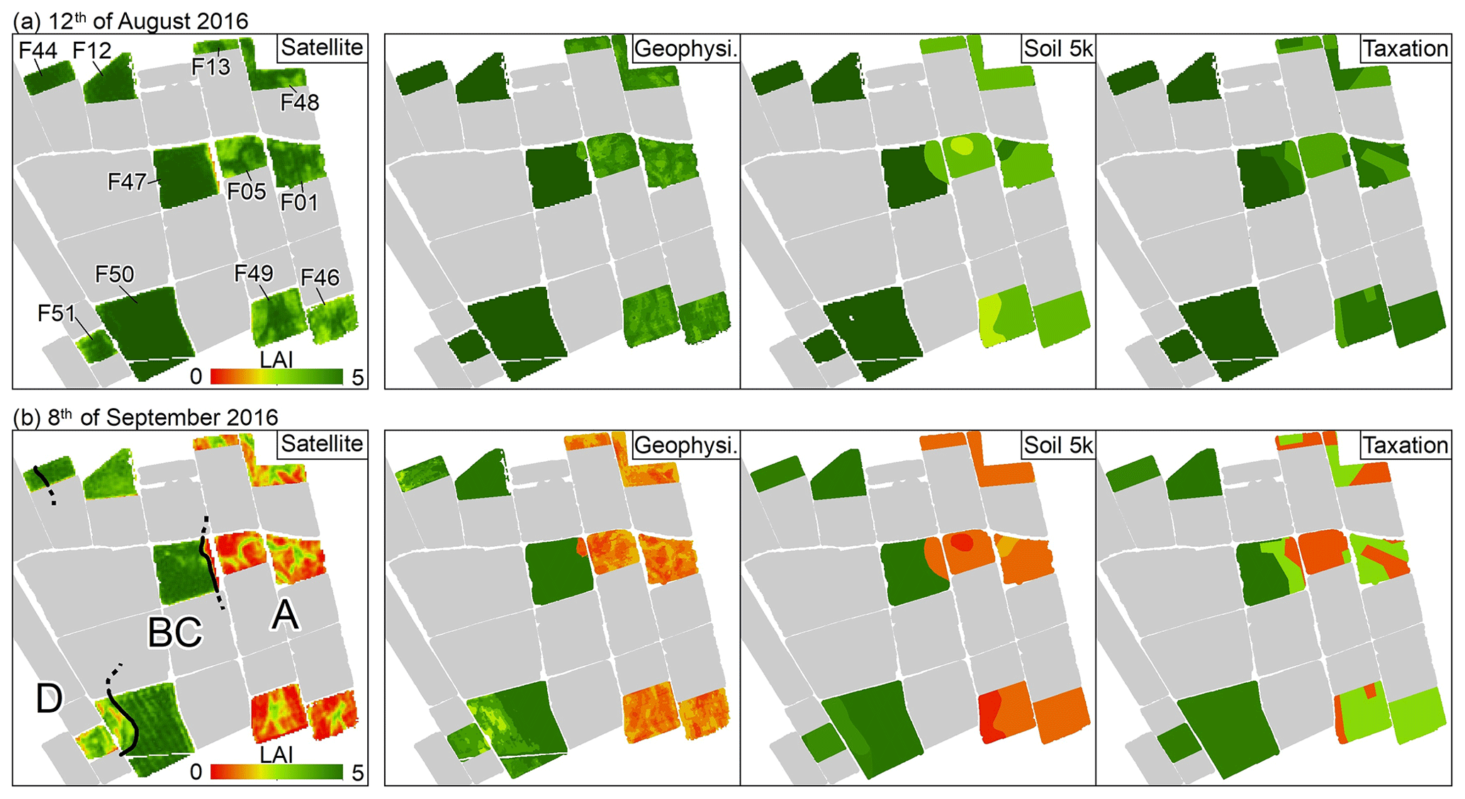
Figure 9Observed LAI_NDVI and simulated LAI obtained using input from the geophysics-based soil map (Geophysi.), the 1 : 5000 soil map (Soil 5k), and the soil taxation map (Taxation); row (a) shows the codes of the investigated fields and the comparison on 12 August 2016, and row (b) shows the geometry of sub-areas A, BC, and D and the comparison on 8 September 2016.

The simulated LAI obtained using the three soil maps captured the large-scale pattern in LAI_NDVI associated with the sub-areas A, BC, and D to some extent. The differences in crop performance between sub-area A and BC were sufficiently well represented in all three simulations. However, the border between low LAI in sub-area A and high LAI in sub-area BC is better represented in the geophysics-based approach (see field F47 in Fig. 9). The differences between the high LAI of sub-area BC and the intermediate LAI of sub-area D were not well represented in the two commonly available soil maps. In fact, the simulated LAI is very similar in the two sub-areas when using the 1 : 5000 soil map and the soil taxation map. This is related to the generally low water stress simulated in sub-area D that did not result in a meaningful reduction of LAI. In contrast, a substantial reduction of LAI was obtained within the simulations based on the geophysics-based soil map. The small-scale patterns in LAI_NDVI observed within each sub-area were also partly captured by the geophysics-based soil map for both dates. In contrast, simulations based on the other two soil maps did not provide results that represented these patterns. At the same time, it is clear that the small-scale variability in LAI_NDVI is not fully captured in our simulation approach because variations within individual soil–crop combinations were not considered.

Table 5RMSE between simulated LAI and LAI_NDVI in fields with sugar beet. The best result for each date is marked in bold.

Download Print Version | Download XLSX

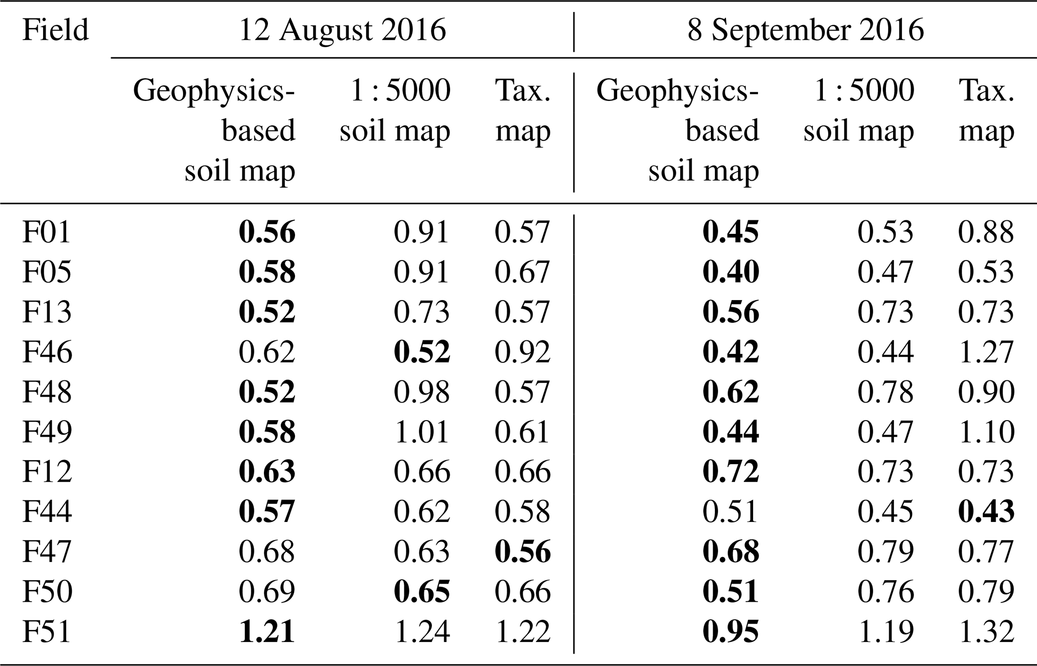
Table 5 provides the pixel-wise RMSE between simulated LAI and LAI_NDVI for all 11 fields where sugar beet was grown. Generally, these fields can be divided into three groups based on the RMSE of each soil map. The first group consists of the fields F01, F05, F13, F46, F48, and F49. In these fields located in sub-area A, the geophysics-based soil map provided improved simulation results for both dates compared to the simulations based on the two other soil maps as indicated by the lower RMSE. Field F46 was the only exception as the lowest values in August (RMSE = 0.52) were obtained with inputs from the 1 : 5000 soil map. In some cases, the difference in RMSE between the simulations based on the three soil maps was rather small, such as in field F48 and field F49. Nevertheless, the RMSE obtained in this group of fields using inputs from the geophysics-based soil map was lower for both days and was larger in September than in August. The second group consists of fields F12, F44, and F47 in sub-area BC. In these fields, no water stress was simulated for any of the soil maps. Therefore, all three soil maps provided accurate LAI simulations, as indicated by the low RMSE. The third group consist of fields F50 and F51 that are located in sub-area D. In August, the RMSE of the simulations performed using the three soil maps was rather similar. In contrast, the simulations based on the geophysics-based soil map clearly outperformed those based on the commonly available soil maps in September. This again corresponds with the simulated water stress in sub-area D, which was high in September but rather low in August.

Overall, the results clearly highlight that the improvements provided by the use of the geophysics-based soil map for the simulation of sugar beet are clearly dependent on the magnitude and timing of water stress. Simulations based on the three soil maps showed rather similar results in periods with sufficient water availability and in areas where water stress did not affect crop development. In contrast, in the presence of significant water stress, the use of the geophysics-based soil map reduced the RMSE between LAI simulations and observations compared with the use of the 1 : 5000 soil map or the soil taxation map. This reduction in RMSE varied substantially from field to field, with a minimum of 2 % and a maximum of 67 %. Likely, this variability is due to local differences in the quality of the soil characterization provided by the three soil maps. The area-averaged RMSE reduction in periods of significant water stress was 25 % compared to the 1 : 5000 soil map and 31 % compared to the soil taxation map.

In field F01 of sub-area A, the reduction of the RMSE between LAI simulations and observations provided by the use of the geophysics-based soil map varied between 15 % and 49 % on 8 September. In this field, the yield recorded by the farmer was 14.2 t ha⁻¹ of dry beet biomass. The use of inputs from the geophysics-based soil map resulted in a simulated yield of 14.3 t ha⁻¹, which was only 1 % higher than the actual yield. The yield simulated with inputs from the commonly available map showed an overestimated yield, with 15.4 ha⁻¹ for the 1 : 5000 soil map (+8 %) and 17.3 ha⁻¹ for the soil taxation map (+22 %). Similarly as in the case of LAI, the geophysics-based soil map outperformed the other two maps. However, these results should be interpreted carefully as the required information was only available for a rather small field within the study area. Nonetheless, it is anticipated that the geophysics-based soil map provides similar improvements in yield estimates as for the LAI simulations for other fields. This expectation is based on the tight relationship between LAI and other aspects of crop development, such as biomass production and ultimately yield. For this same reason, the assimilation of LAI data into crop growth model ensembles has been shown to improve yield estimates (Jonckheere et al., 2004; Tewes et al., 2020; Wilhelm et al., 2000).

When comparing the results provided by the use of the three maps, it has to be noted that the geophysics-based soil map was produced with a set of 100 sampling locations (one per hectare), which is similar to the sampling density of the 1 : 5000 soil map (∼ one per hectare) and lower than the one of the soil taxation map (∼ four per hectare). It can be argued that the geophysics-based soil map had an advantage resulting from the quantitative textural information based on laboratory analysis. To a certain extent, this holds true. However, it should be seen against the background that textural information on the coarse soils from the geophysics-based product was integrated into the simulations with the commonly available soil maps. Furthermore, the characterization of the upper soils only showed local differences between the three maps.

The reduction in performance of the 1 : 5000 soil map and of the soil taxation map compared to the geophysics-based soil map was strongly dependent on local soil characteristics. In general, it was found that this reduction in performance was caused by a poor representation of (i) the spatial geometry of individual soil units, (ii) the depth to the coarse sediments, (iii) the textural characteristics of the overlying sediments, and (iv) the subdivision between large sub-areas. The different quality of this soil representation affected the quality of the LAI simulations throughout the year and especially towards the end of the growing season of the summer crops.