Trigonometric Embeddings in Polynomial Extended Mode Decomposition—Experimental Application to an Inverted Pendulum

Abstract

The extended dynamic mode decomposition algorithm is a tool for accurately approximating the point spectrum of the Koopman operator. This algorithm provides an approximate linear expansion of non-linear discrete-time systems, which can be useful for system analysis and controller design. The accuracy of this algorithm depends heavily on the availability of a set of basis functions that provide the ability to capture the nonlinear dynamics of the underlying system. Recently, the use of orthogonal polynomials, along with reduction techniques for the dimension and maximum order of the polynomial basis, have been successfully used to approximate nonlinear systems with the additional benefit of using smaller datasets. This paper expands the current methods for selecting the set of observables for nonlinear systems with periodic behavior, which is prone to a representation in terms of trigonometric functions. The benefit of working with orthogonal polynomials is preserved by embedding the trigonometric functions into the orthogonal basis. The algorithm is illustrated with the data-driven modelling of an inverted pendulum in simulation and real-life experiments.

1. Introduction

Recent developments for the analysis and control of nonlinear systems focus on the properties of linear transformations of these systems [1], such as the Koopman operator [2]. Although this latter transformation is infinite dimensional, there are approximation methods that allow for capturing the point spectrum of the operator based on datasets that were collected from the nonlinear system. The prevalent technique to perform this finite dimensional approximation is the dynamic mode decomposition (DMD) [3], and its generalization, the extended dynamic mode decomposition (EDMD) [4,5], which can make use of a variety of dictionaries of observable functions spanning subspaces over which the Koopman operator can be approximated. The main advantage of these techniques is the ability to analyze the spectral decomposition of the regression matrix or Koopman matrix [6,7,8,9,10,11,12,13]. An additional advantage is the possibility to include the forcing signals of the system into the transformation in view of its control [14,15,16,17]. These latter developments make use of model predictive control (MPC), but the availability of the Koopman matrix and its spectral decomposition should allow the extension of classical linear control techniques to the linear evolution of observables.

A key aspect is the selection of the observables to capture complex dynamics and avoid excessive data requirement. For example, the sparse identification on the non-linear dynamics (SINDY) algorithm [18] starts with a dictionary of observables and performs a sparse regression by regularized least squares on the original state variables of the system to identify the ones that best describe the dynamics. An alternative is the EDMD algorithm with dictionary learning [19] (EDMD-DL), where, instead of starting with a predefined set of observables, the algorithm iterates between learning a dictionary via an artificial neural network, and the approximation of the Koopman matrix via traditional EDMD. These techniques have the advantage of reducing the dimension of the set of observables, and possibly the requirement for data to approximate the dynamics. In addition to these techniques, a common practice is to use norm-based expansions, radial-basis functions, kernel-based [20], orthogonal polynomials, and their variations [16]. Conversely, these methods have some numerical stability problems when dealing with the set of observables. All of these must deal with the problem of recovering the state, and, for this purpose, a common practice is to include the state in the set of observables, at the cost of the possibility of not having a basis that spans the function space that is necessary for an accurate approximation. When the inclusion of the state is not the case, the solution is to solve a second optimization problem that finds the best projection matrix of the state onto the set of observables. The problem of this approach is the addition of an additional algebraic step that relies on the accuracy of a pseudo inverse, again, at the cost of the possibility of this matrix not spanning the state space.

In a previous work of the authors [12], an improvement of the EDMD algorithm is proposed through the use of orthogonal polynomials and a p-q-quasi norm reduction method, coupled with a selection procedure for the best p-q values. This algorithm allows for a set of observables that is a basis and, therefore, solves the drawbacks of traditional methods and does not require the solution of a second optimization problem to recover the state. The basis reduction and the preservation of the spectrum can be achieved based on a small dataset. Even though the technique achieves good performance for systems that have a polynomial structure in the underlying dynamics, or systems with periodic behavior, where the evolution of states has trigonometric components, the polynomial methods offer room for improvement.

The main contribution of this study is to embed trigonometric functions [21], or any particular functions, into the orthogonal polynomial basis in order to better represent systems with cyclic behavior, respectively, any particular behavior. These embeddings improve the accuracy of the algorithm, while preserving the advantage of the reduction method previously introduced in [12]. The performance of the approach is demonstrated in simulation and real-life experiments with an inverted pendulum on a cart.

This paper is organized, as follows. The next section introduces the EDMD algorithm along with some recent improvements that allow the use of reduced orthogonal basis for its computation. Section 3 describes the concept of embedding trigonometric functions, or any kind of function into the state space of the system to exploit the a priori knowledge of a variable behavior. Section 4 illustrates how these embeddings perform by modeling a pendulum on a cart. Finally, Section 5 gives some analysis and conclusions.

Notation$\mathbb{C}$ denotes the field of complex numbers. $\mathbb{R}$ and ${\mathbb{R}}_{+}$ denote the field of real and nonnegative real numbers, respectively. For any matrix $A\in {\mathbb{R}}^{n\times n}$, $A^{\top }$ denotes transpose, $A^{+}$ denotes its pseudoinverse, and $\left|\right|x\left|\right|$ represents the Euclidean norm. For a complex number $\lambda$, $\left|\lambda \right|$ represents its absolute value. For any set A, $\overline{A}$ denotes the closure of A. The vector exponentiation $M^{\pm \eta }$ is defined term by term. A level set of an arbitrary function $h\left(x\right)$ for any constant c is $\Gamma \left(h\left(x\right)\right)=\{x\in {\mathbb{R}}^n:h\left(x\right)=c\}$.

2. Preliminaries

The extended dynamic mode decomposition (EDMD) algorithm [5] is a numerical procedure closely related to modern data-driven and machine learning techniques, where the information comes either from the numerical integration of a nonlinear differential equation system or from the measurements of real system variables. This has to be contrasted with traditional system identification techniques that rely upon both the explicit knowledge of the differential equation model [22,23,24] and gathered experimental data. Because EDMD is the backbone of the linear predictors developed in this study, this section presents a description of the algorithm along with its improvements and shows via simulations of the pendulum on a cart its advantages over the current alternative methods.

Consider the non-autonomous nonlinear system $(\mathcal{M},\mathcal{U},T(x,u),k)$ in discrete time, with state variables $x\in \mathcal{M}$, where $\mathcal{M}\subseteq {\mathbb{R}}^n$ is the nonempty compact state space, forcing signals $u\in \mathcal{U}$, where $\mathcal{U}\subseteq {\mathbb{R}}^r$ is the nonempty compact input space, $k\in {\mathbb{Z}}_0^{+}$ is the discrete time, and $T:\mathcal{M}\times \mathcal{U}\to \mathcal{M}$ is the differentiable vector-valued evolution map, i.e.,

$$x(k+1)=T\left(x\right(k),u(k\left)\right),$$

(1)

where a trajectory, or an orbit of the system is the sequence of states ${\left(x_i\right)}_{i=0}^k$ that come from the solution of (1), which is the successive application of the non-linear mapping T from an initial condition $x_0\in \mathcal{M}$ at $k=0$ and a specific sequence of forcing signals $u\triangleq {\left(u_i\right)}_{i=0}^{k-1}$.

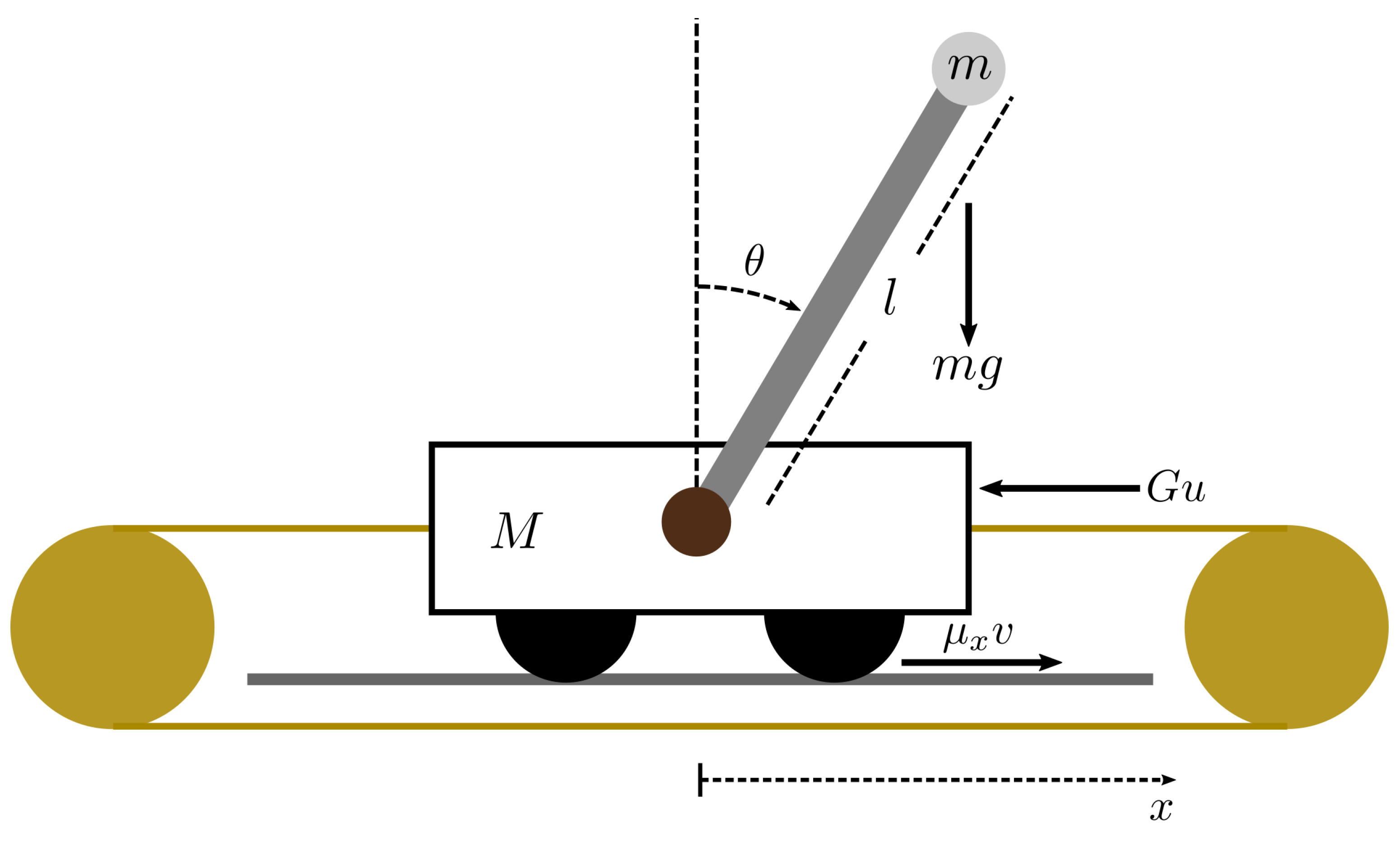
For example, consider the experimental set-up that will be used later on in this study for the validation of the trigonometric embeddings. The system consists of a pendulum and a moving cart attached by a swivel that allows the pendulum to rotate freely. The cart wheels rotate on a rail and a DC motor drives the whole system. The available information from two encoders are the displacement of the cart and angular rotation of the pendulum. Figure 1 depicts the experimental set-up, where x is the horizontal displacement of the cart and $\theta$ is the angle of the pendulum with respect to the vertical axis. Mass and energy balances give a set of ordinary differential equations that describe the dynamics of the system.

The system equations, which depend on the masses of the cart and pendulum, the length of the pendulum rod, the linear damping of the cart wheels with the rails, and the gravitational constant, are given by

$$\begin{array}{cc}\hfill \dot{x}& =v\hfill \\ \hfill \dot{v}& =\frac{Gu-{\mu }_{x}v-ml{\theta }_v^{2}sin\left(\theta \right)}{M+m{sin}^2\left(\theta \right)}\hfill \\ \hfill \dot{\theta }& ={\theta }_v\hfill \\ \hfill {\dot{\theta }}_v& =\frac{Gu-{\mu }_{x}v-ml{\theta }_v^{2}sin\left(\theta \right)cos\left(\theta \right)+(M+m)gsin\left(\theta \right)}{l-ml{cos}^2\left(\theta \right)},\hfill \end{array}$$

(2)

where the states are the cart displacement x, the cart velocity v, the rod angle $\theta$, and the angular velocity ${\theta }_v$. The model also considers a gain G between the voltage of the motor u and the resulting force on the cart. The parameter of the model come either from the available data from the manufacturer (Feedback Instruments Ltd. Crowborough, UK) or from an identification of the parameter from a set of data collected in preliminary experiments with the system.

Table 1. Parameters of the inverted pendulum on a cart.

	Description	Value	Units
M	Cart Mass	1.12	$\left[\mathrm{kg}\right]$
m	Pendulum Mass	0.0905	$\left[\mathrm{kg}\right]$
g	Gravity	9.81	$[\mathrm{m}·{\mathrm{s}}^{-2}]$
l	Pendulum length	0.365	$\left[\mathrm{m}\right]$
${\mu }_x$	Cart Friction	6.65	$[·]$
G	Tension-Force Gain	7.5	$[·]$

lists the value of these parameters.

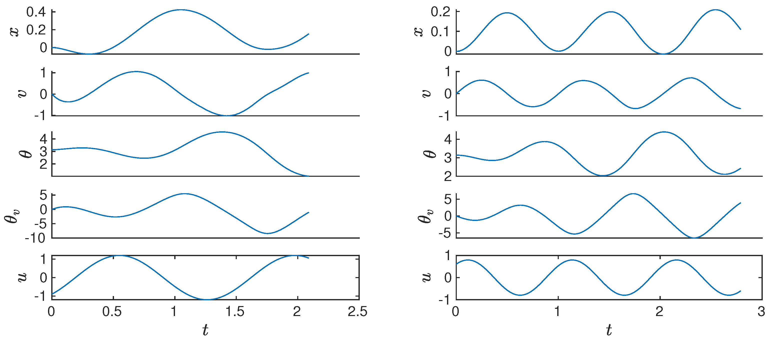
Let us now consider a set of seven orbits or trajectories that were obtained by the numerical integration of (2) with the assumption that all of the state variables of the system are available. For the accuracy of the algorithm, it is necessary that the trajectory samples are collected at a constant rate, which is chosen equal to 0.01 s, in both the numerical simulation and experimental study. This set of orbits sampled at a constant $\Delta t$ correspond to the solution of the non-linear discrete-time mapping (1).

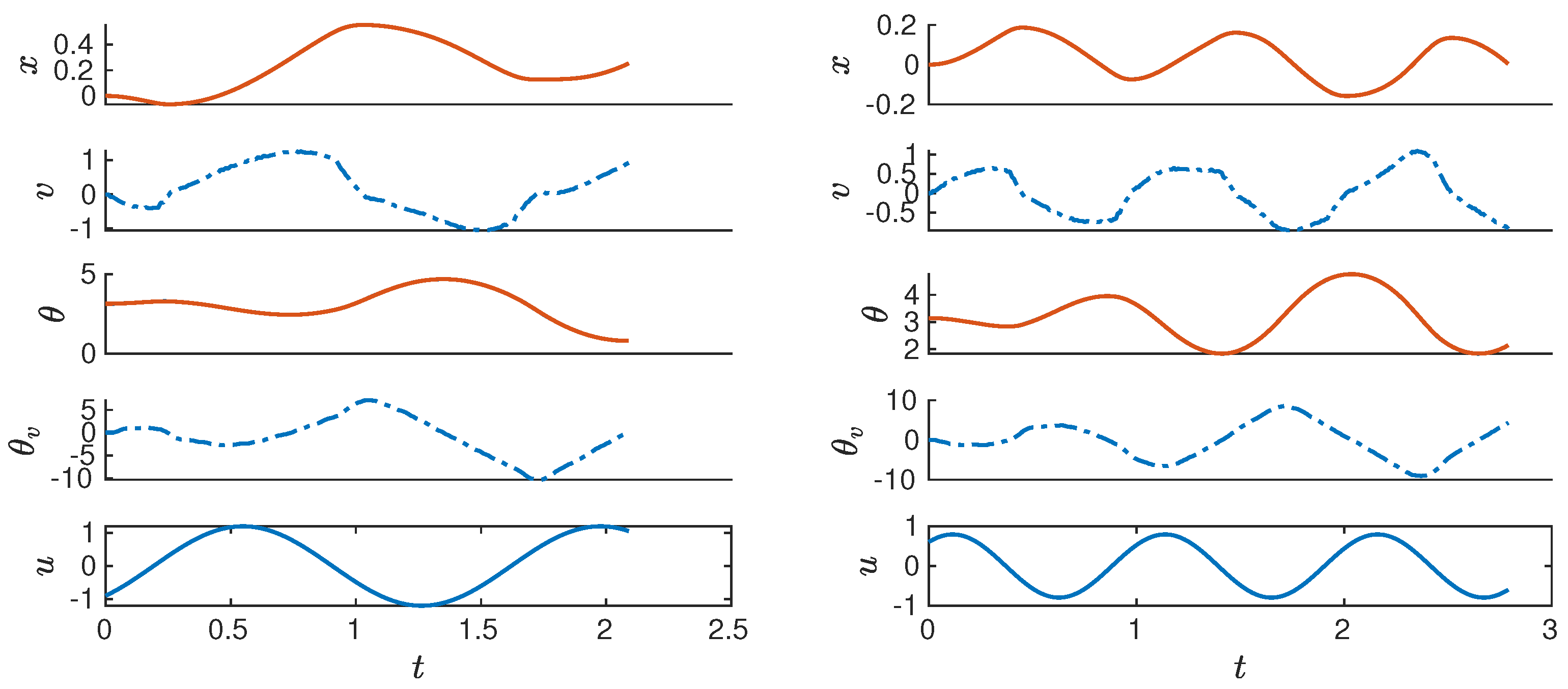
Figure 2 depicts the discrete-time evolution of some of these trajectories with their respective forcing signals. These trajectories serve as the available data to approximate the non-linear dynamics via the EDMD algorithm.

Because EDMD is a data-driven approach, the set of trajectories is divided into training and testing sets for the approximation and validation of the algorithm. In our case study, the selection is five orbits for training the linear predictor, and two for testing (Figure 2). Finally, the snapshot data are defined as a set of tuples $\left\{(x_i,y_i,u_i)\right\}$, where $y_i=T(x_i,u_i)$. From these tuples, the snapshot matrices are given by:

$$X=\left[\begin{array}{ccc}{x}_1& \cdots & x_N\end{array}\right],Y=\left[\begin{array}{ccc}{y}_1& \cdots & y_N\end{array}\right],U=\left[\begin{array}{ccc}{u}_1& \cdots & u_N\end{array}\right],$$

(3)

according to the traditional EDMD algorithm [5] and the extension for including the inputs of the system [17]. The rationale behind the approach is to obtain linear predictors of the state evaluated on a vector-valued function of observables $\Psi \left(x\right)={[{\psi }_1\left(x\right),\dots ,{\psi }_d\left(x\right)]}^{\top }:\mathcal{M}\to {\mathbb{C}}^{d\times 1}$ where d is the dimension of the set of observables that must satisfy the condition

$$\Psi \left(y\right)=U_{d,x}\Psi \left(x\right)+U_{d,u}u+r(x,u)$$

(4)

$r(x,u)\in \mathcal{F}$ is the residual term that has to be minimized in order to find matrices $U_{d,x}$ and $U_{d,u}$. This leads to the least squares problem

$${\parallel r(x,u)\parallel }^2=\frac{1}{N}\sum _{i=1}^N\frac{1}{2}{∥\Psi \left(y_i\right)-U_{d,x}\Psi \left(x_i\right)-U_{d,u}u∥}_2^2,$$

(5)

which as a closed-form solution

$$\left[\begin{array}{cc}{U}_{d,x}& U_{d,u}\end{array}\right]=\Psi \left(Y\right){\left[\begin{array}{c}\Psi \left(X\right)\\ U\end{array}\right]}^{\top }{\left(\left[\begin{array}{c}\Psi \left(X\right)\\ U\end{array}\right]{\left[\begin{array}{c}\Psi \left(X\right)\\ U\end{array}\right]}^{\top }\right)}^{-1}.$$

(6)

Because the purpose of these predictors is the synthesis of controllers, it is necessary to recover the state from the observable functions. Thus, an additional least squares problem for the best projection matrix of x onto the span of $\Psi$ has to be solved. The projection must satisfy the condition

$$\overline{x}=U_{d,c}\Psi \left(x\right)+r_c\left(x\right),$$

(7)

where $r_c\left(x\right)$ is the residual term to be minimized to find $U_{d,c}$, which accepts a pseudo-inverse based least squares solution

$$U_{d,c}=X\Psi {\left(X\right)}^{+}.$$

(8)

Instead of solving (8) to recover the state, a common practice is to include the state in the set of observables, so that matrix $U_{d,c}=[I_n,0_{n\times (d-n)}]$ after reordering the observables, such that the state vector forms the first n elements.

The EDMD formulation (6) and (8) can be used with a basis of Jacobi type monomials for the approximation of the pendulum dynamics (2), i.e., a sequence of orthogonal polynomials ${\left\{{\pi }_{\alpha }\left(x\right)\right\}}_{\alpha =0}^p$ where ${\pi }_{\alpha }\left(x\right)$ is a univariate polynomial (i.e., a polynomial in only one of the state variables $x_i$, $i=1,\dots ,n$) of degree $\alpha \in {\mathbb{N}}_{+}$ up to order p. This sequence is defined over a range $[a,b]$, where some inner product between distinct elements is zero, i.e., $\langle {\pi }_i\left(x\right),{\pi }_j\left(x\right)\rangle =0$ for $i\ne j$, and it satisfies a particular ordinary differential equation. Each element of the observable basis is the tensor product of n univariate polynomials,

$${\psi }_l\left(x\right)=\prod _{j=1}^n{\pi }_{{\alpha }_j}\left(x_j\right)l=1,\dots ,d.$$

(9)

For the approximation of the pendulum dynamics, the order $p=1$ can be chosen, giving a set of observables of dimension $d=17$ (16 for the state and 1 for the input) with maximum order 4, i.e., the last observable of the state is the product of all the univariate monomials ${\psi }_{16}={\prod }_{i=1}^{4}5x_i+1$ for parameters $a=5$ and $b=3$ of a Jacobi type monomial of order one in the variable x, $J(1,a,b,x)=a/2-b/2+x(a/2+b/2+1)$. When considering the pendulum states,

Table 2. Indices for the state observables.

	${\mathit{\psi }}_{\mathbf{1}}$	${\mathit{\psi }}_{\mathbf{2}}$	${\mathit{\psi }}_{\mathbf{3}}$	${\mathit{\psi }}_{\mathbf{4}}$	${\mathit{\psi }}_{\mathbf{5}}$	${\mathit{\psi }}_{\mathbf{6}}$	${\mathit{\psi }}_{\mathbf{7}}$	${\mathit{\psi }}_{\mathbf{8}}$	${\mathit{\psi }}_{\mathbf{9}}$	${\mathit{\psi }}_{\mathbf{10}}$	${\mathit{\psi }}_{\mathbf{11}}$	${\mathit{\psi }}_{\mathbf{12}}$	${\mathit{\psi }}_{\mathbf{13}}$	${\mathit{\psi }}_{\mathbf{14}}$	${\mathit{\psi }}_{\mathbf{15}}$	${\mathit{\psi }}_{\mathbf{16}}$
x	0	1	0	1	0	1	0	1	0	1	0	1	0	1	0	1
v	0	0	1	1	0	0	1	1	0	0	1	1	0	0	1	1
$\theta$	0	0	0	0	1	1	1	1	0	0	0	0	1	1	1	1
${\theta }_v$	0	0	0	0	0	0	0	0	1	1	1	1	1	1	1	1

shows the set of indices $\alpha$ for each of the observables of the state.

Note that Table 2 shows a base $p+1$ counting solution with n significant figures, so that the base 10 digits from zero up to ${(p+1)}^n-1$ in a $p+1=2$ base is given by

$$\begin{array}{cc}\hfill {\left(\begin{array}{ccc}0,& 1,\dots ,& {(p+1)}^n-1\end{array}\right)}_{\mathrm{base}p+1}& ={\left(\begin{array}{ccc}0,& 1,\dots ,& 15\end{array}\right)}_{\mathrm{base}2}\hfill \\ \hfill & =\left(\begin{array}{cccc}0000,& 0001,& \cdots ,& 1111\end{array}\right).\hfill \end{array}$$

This set of indices has a simple computational solution using Matlab, not only for generating it, but also as an input for the subsequent reductions. Along with the set of indices, and the method for generating the basis as a tensor product of the univariate polynomials from (9), the orthogonal basis is

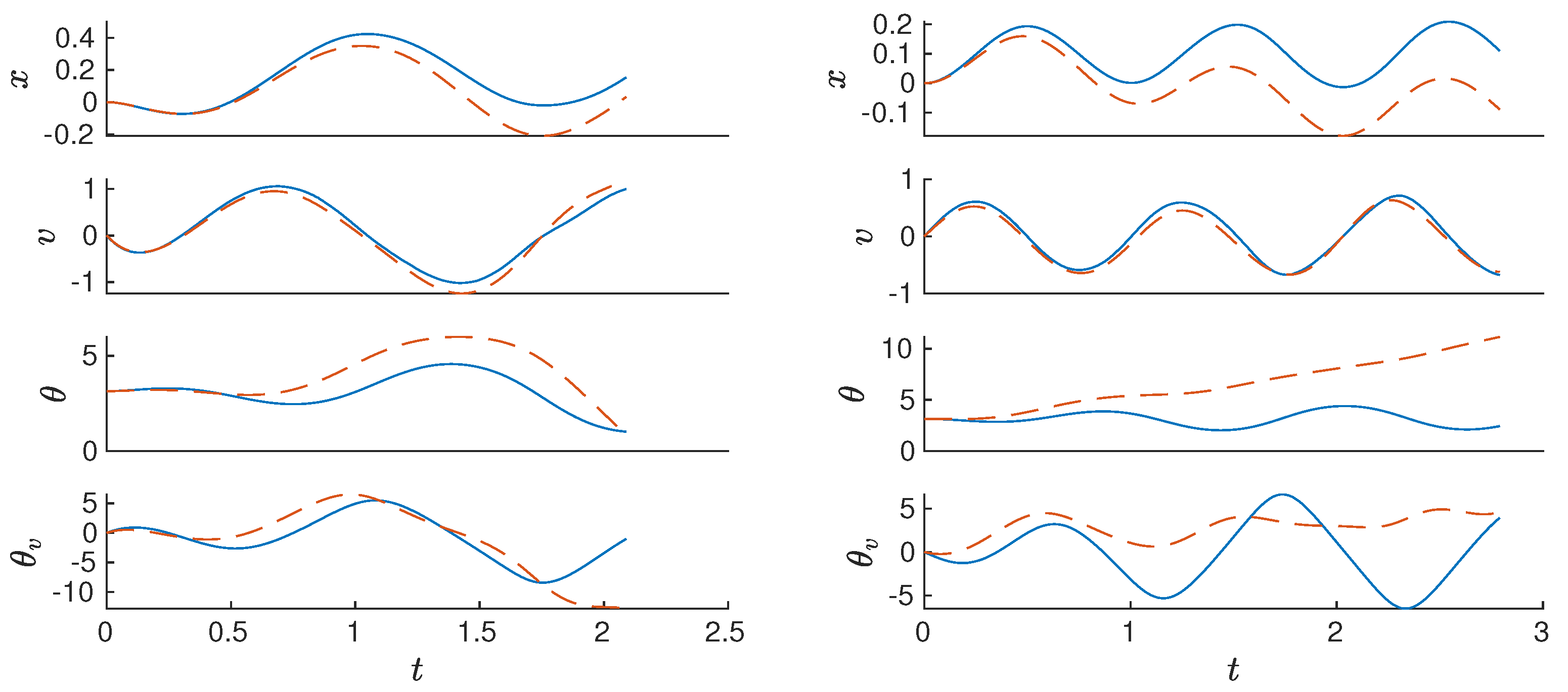
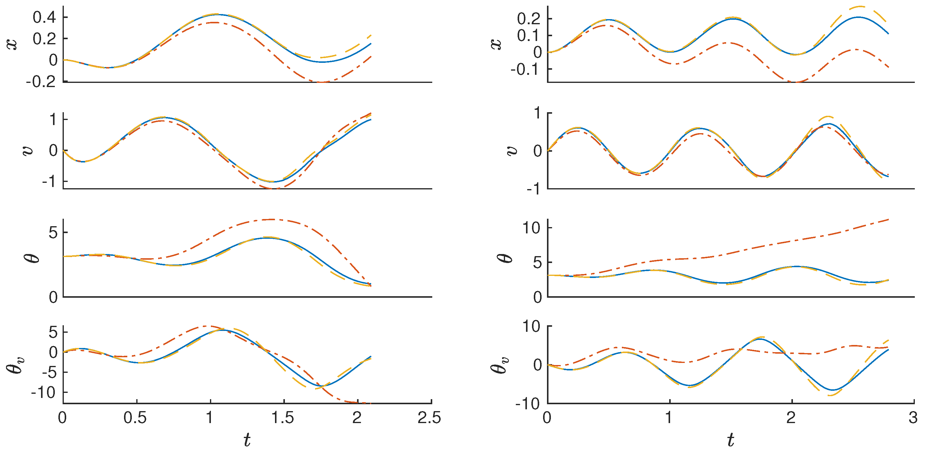
When considering five trajectories of the training set that sum 1110 data points, two trajectories of the testing set that sum 490 data points, and a Jacobi type set of polynomials, the solution of the EDMD algorithm gives a linear predictor of the extended state. Figure 3 shows the trajectories that were produced by the EDMD, where the mean absolute error $ϵ=1/N{\sum }_i^N|x_i-{\overline{x}}_i|$ is 1.31, and the max absolute error ${ϵ}_M=\max |x_i-{\overline{x}}_i|$ is 11.79. While it is possible to perform the approximation with higher p values, the results do not necessarily improve. For $p=2$, as the maximum order of the univariate polynomials, the basis has dimension $d=81$ with a maximum order of eight, which shows that these two numbers grow exponentially with the maximum univariate order p. Moreover, in this particular case the mean absolute error increases to 1.77, which is also a sign of numerical issues due to the maximum order, even though the maximum absolute error decreases to 8.43.

Indeed, there are some inherent numerical instabilities with the method. First, the EDMD algorithm is a linear map on the function space that the set of observables span, and the accuracy of the solution depends on the characteristics of this set. Choosing an orthogonal basis with an observable that corresponds to a constant generally improves the performance of the approximation. In contrast, adding the state to the set of observables is prone to breaking the orthogonality of the observables, depending on their actual choice. As a consequence, the square matrix ${[\Psi (X),U]}^{\top }[\Psi \left(X\right),U]$ in (6) becomes singular or close to singular and, while replacing the inverse by a Moore–Penrose pseudo inverse can partly alleviate this issue, the result can still be inaccurate. Second, preserving an orthogonal basis, without explicitly including the states as observables poses a similar matrix inversion problem, when there is no solution to the projection of the state space onto the set of observables.

The way out of this dilemma is the selection of order-one, univariate, injective, polynomial elements for the recovery of the state [13], which implies that there is no need for breaking the orthogonality of the set while still being able to recover the state as a linear function of the observables, completely avoiding the burden of a matrix inversion.

Besides, the exponential growth of the maximum order and dimension of the set of observables based on orthogonal polynomial has a solution via p-q-quasi norms and polynomial accuracy methods.

The reduction by p-q-quasi norms (the quantity ${\parallel ·\parallel }_q$ is not a norm because it does not satisfy the triangle inequality) [25] is the truncation of higher order elements from the basis by defining the q-quasi norm

$${\parallel \alpha \parallel }_q={\left(\sum _{i=1}^n{\alpha }_i^q\right)}^{\frac{1}{q}},$$

(10)

and by defining a maximum degree $p\in \mathbb{N}$ and a quasi norm $q\in {\mathbb{R}}_{+}$ to obtain a set of indexes $\alpha =\{\alpha \in {\mathbb{N}}^n:\parallel \alpha {\parallel }_q<p\}$, which defines the order of each of the univariate polynomial elements whose products form the elements of the observables. With this truncated set of indices, every element of the vector valued function of observables is the tensor product of n univariate polynomials, as in (9). When considering the previous Matlab code example, the necessary modification consists in the addition of one line of code that performs the truncation before calculating the univariate polynomials.

The result of the truncation has as a consequence that different values of q for a particular value of p give the same basis of polynomials. As the current method to determine the best p-q combination is a sweep over the parameters, it is necessary to determine the equivalent sets of parameters before calculating the different EDMD algorithms in order to avoid the computational burden of calculating the same EDMD for an equal basis. Moreover, the sweep over the parameters is a process that achieves a sub-optimal solution because an optimal selection based on the dynamics of the system or the analysis of the data samples is still an open question. The only limitation on the selection of the sweep is in terms of the computational burden from the exponential growth of the dimension of the basis according to the p-q parameters. when considering this limitation, the full set of indices $\alpha$ without truncation has the potential of becoming too big for the computers memory In this case, it is possible to revert the matrix-based calculation of the truncated indices to an element-wise process, adding at least two orders of magnitude to the required time to complete the process. Along with this limitation, the dimension of the polynomial basis is also computationally taxing on the inverse or pseudo inverse in (6).

The vector valued function of observables can be further reduced by considering the polynomial accuracy

$${ϵ}_l=\frac{1}{N}\sum _{i=1}^N\frac{|{\psi }_l\left(y_i\right)-U_{d_l}{\psi }_l\left(x_i\right)|}{|{\psi }_l\left(y_i\right)|},l=1,\dots ,n$$

(11)

where $U_{d_l}$ is the l-th row of the EDMD matrix.

Because the n injective order-one univariate elements have to remain in the basis, so as to be able to recover the state later on, the threshold $\overline{ϵ}$ for the elimination of elements is the maximum of the errors with an alpha index equal to one

$$\overline{ϵ}=max(ϵ:\parallel {\alpha }_l{\parallel }_1=1),$$

(12)

and the multivariate polynomial elements that stay in the reduced vector-valued function of observables ${\Psi }_R\left(x\right)$ are

$${\Psi }_R\left(x\right)=\{\Psi \left(x\right):ϵ\le \overline{ϵ}\}.$$

(13)

Above this threshold, the corresponding observables are discarded. Consequently, a reduction of the mean absolute error is expected.

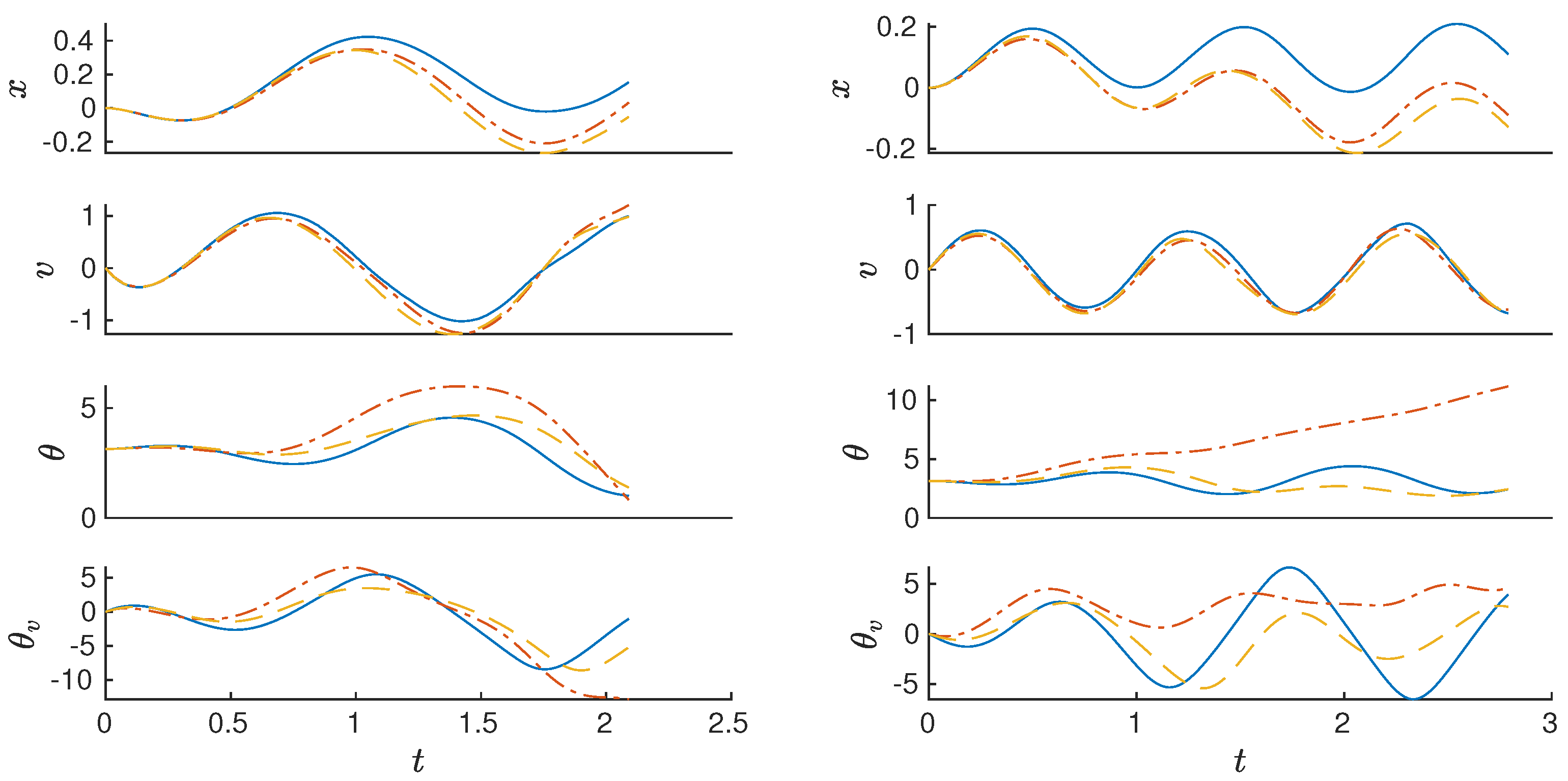
In our case study of the inverted pendulum, we can consider the same orthogonal basis of Jacobi polynomials with a sweep of p-q parameters corresponding to: $p=[2,3,5,]$ and $q=[0.3,0.5,0.7,0.9,1.1,1.3]$. Although there are 18 possible combinations, some p-q parametrizations produce equal basis. There are only 12 distinct sets of observables, ranging from six elements of maximum order 2 to 173 elements of maximum order 5. The result of the reduction gives a sub-optimal basis of 33 elements of maximum order 3 that achieves a mean absolute error of 0.62 and a maximum absolute error of 4.85, as compared to 1.31 and 11.79 for the traditional EDMD. Note that the reduction provides the possibility to test higher-order polynomial basis than in the traditional form, where a basis of maximum order 5 would count 625 elements. In addition to the versatile selection of higher order polynomial basis, the p-q-EDMD also reduces the necessary amount of data for producing accurate linear predictors (in our case study, the algorithm needs 1110 data points for the training set). This reduction allows the implementation of the algorithm in real systems, where it is expensive and time consuming to acquire big data-sets. 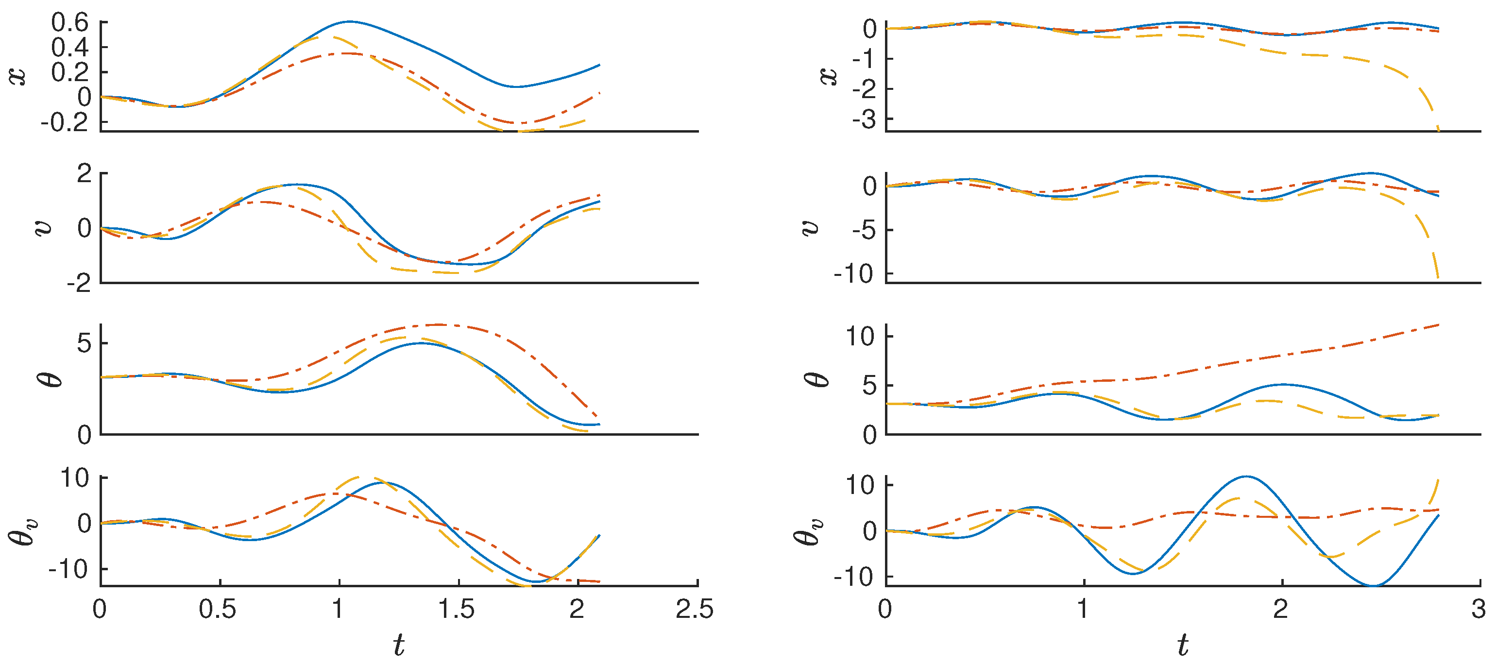Figure 4 shows the performance of the sub-optimal basis of the p-q-EDMD in comparison to the traditional EDMD.

Although the use of reduced orthogonal polynomials for the p-q-EDMD provides a method for improving the accuracy of the algorithm while avoiding computationally heavy high-order and dimensional solutions, the accuracy of the algorithm for systems that have trigonometric components or an arbitrary behavior, like exponentials or logarithms, is not enough. Therefore, the next section introduces the concept of trigonometric embeddings.

3. Trigonometric Embeddings

In this section, we consider the problem of representing dynamic systems with oscillatory behavior by polynomial expansions and the possibility to increase the parsimony of the approximation by the inclusion of trigonometric functions as elementary units of the polynomial expansion. Similar embeddings could be used for any particular behavior, using associated functions. Similar to the idea that took the dynamic mode decomposition algorithm to the extended version, where, instead of performing a regression on the states, the extended method considers a set of functions of the state (the so-called observables), the trigonometric embeddings, or more generally function embeddings, provide specific functions of the state conveying particular information.

Consider the discrete-time dynamical system (1) and assume that a subset m of the state $x^{tg}\subseteq x$ has trigonometric components in the difference equation $T(x,u)$. For each of these state variables, an extension of the state vector is achieved with 2 additional variables, leading to

$$x_e=\left[\begin{array}{c}{x}_1\\ ⋮\\ x_n\\ x_{e_1}\\ ⋮\\ x_{e_{2m}}\end{array}\right],$$

(14)

where $m\le n$ and $x_e$ belongs to some extended space, i.e., $x_e\in {\mathcal{M}}_e$ where ${\mathcal{M}}_e\subseteq {\mathbb{R}}^{n+2m}$. In this extended space, a set of observables $\Psi \left(x_e\right)={[{\psi }_1\left(x_e\right),\dots ,{\psi }_d\left(x_e\right)]}^{\top }:{\mathcal{M}}_e\to {\mathbb{C}}^{d\times 1}$ is defined, where each element comes from (9), with the same p-q-quasi norm reduction (10) of the p-q-EDMD algorithm. Therefore, preserving the advantages of working with a reduced orthogonal basis.

Consider, for example, an arbitrary discrete-time dynamical system $(\mathcal{M},\mathcal{U},T(x,u),k)$, where $n=2$, $r=2$ and $x^{tg}=x_2$, i.e., the system has two state variables where the second one has a trigonometric component and two inputs within the non-linear mapping $T(x,u)$. Moreover, a Hermite basis of orthogonal polynomials of univariate elements up to order 2, i.e., ${\pi }_{\alpha =[0,1,2]}\left(x\right)=[1,2x,4x^2-2]$, is used. For illustration purposes, assume an arbitrary p-q parametrization $p=3$ and $q=0.7$. The resulting polynomial basis of the extended space is

$$\Psi \left(x_e\right)=\left[\begin{array}{c}1\\ 2x_1\\ 4x_1^2-2\\ 2x_2\\ 4x_1{x}_2\\ 4x_2^2-2\\ 2x_{e_1}\\ 4x_1{x}_{e_1}\\ 4x_2{x}_{e_1}\\ 4x_{e_1}^2-2\\ 2x_{e_2}\\ 4x_1{x}_{e_2}\\ 4x_2{x}_{e_2}\\ 4x_{e_1}{x}_{e_2}\\ 4x_{e_2}^2-2\end{array}\right].$$

(15)

To bring the set of observables from the extended space into the original state space of the system, the following transformation has to be applied,

$$\begin{array}{cc}\hfill x_{e_i}& =cos{x}_i^{tg}\hfill \\ \hfill x_{e_{i+1}}& =sin{x}_i^{tg},\hfill \end{array}$$

(16)

for $i=1,\dots ,m$. In our case study, the set of observables of the state becomes

$$\Psi \left(x\right)=\left[\begin{array}{c}1\\ 2x_1\\ 4x_1^2-2\\ 2x_2\\ 4x_1{x}_2\\ 4x_2^2-2\\ 2cos\left(x_2\right)\\ 4x_{1}cos\left(x_2\right)\\ 4x_{2}cos\left(x_2\right)\\ 4{cos}^2\left(x2\right)-2\\ 2sin\left(x_2\right)\\ 4x_{1}sin\left(x_2\right)\\ 4x_{2}sin\left(x_2\right)\\ 4cos\left(x_2\right)sin\left(x_2\right)\\ 4{sin}^2\left(x_2\right)-2\end{array}\right].$$

(17)

Note that the embeddings are not restricted to trigonometric functions, but could, for instance, include logarithmic, exponential, or hyperbolic functions, if the non-linear mapping $T(x,u)$ has state variables with such a behavior. However, the functional embeddings and, particularly the trigonometric embeddings, which add two more variables for each trigonometric state, exponentially increases the dimension of the set of observables and it is necessary to resort to the previous p-q-quasi norm reduction.

The application of trigonometric embeddings to the orbits of the pendulum problem, when considering that only the angle $\theta$ has trigonometric components, reduces both error metrics, the mean absolute error of the approximation, from the aforementioned value of 0.62 (provided by p-q-EDMD) to 0.17 and the maximum absolute error from 4.85 to 2.46. To achieve these results, we consider a p-q sweep where $p=[2,3,4,5]$, $q=[0.3,0.5,0.7,0.9,1.1,1.3]$ and the available orthogonal polynomials in Matlab.

Table 3. Mean and max absolute errors for each polynomial basis used in the p-q Trigonometric; EDMD.

Polynomial Basis	$\mathit{ϵ}$	${\mathit{ϵ}}_{\mathit{M}}$
Hermite	0.2008	2.6163
Legendre	0.2108	3.3836
Laguerre	0.1712	2.4686
ChebyshevT	0.2211	3.8535
ChebyshevU	0.2163	2.4432
Gegenbauer	0.1916	2.5652
Jacobi	0.2092	3.6033

shows the mean absolute errors and the maximum absolute errors for the best sub-optimal solution for each polynomial basis. The sub-optimal solution is a Laguerre polynomial basis with parameters $p=4$ and $q=0.7$. Although the approximation error in the test set is reduced, the inclusion of the two extra trigonometric variables and the increased p value produce a basis of 65 elements. Figure 5 depicts the result of the algorithm in comparison with the benchmark EDMD.

4. Inverted Pendulum: Experimental Results

For illustration purposes, and to compare numerically various expansions, we consider the real-life application that was provided by a Feedback Digital Pendulum 33-005-PCI (Figure 6).

This pendulum is the same as that described in Section 2. A DC motor drives the cart along the rail to which a pendulum is attached. The available experimental set-up provides, through two encoders, the noisy measurements of the cart position, and the pendulum angle every 0.01 [s]. Therefore, the output equation is given by:

$$y=\left[\begin{array}{cccc}1& 0& 0& 0\\ 0& 0& 1& 0\end{array}\right]\left[\begin{array}{c}x\\ v\\ \theta \\ {\theta }_v\end{array}\right]+w_n,$$

(18)

where $w_n\sim \mathcal{N}(0,{\sigma }^2)$.

However, the knowledge of the cart velocity and the angular velocity are necessary for computing an approximation through the EDMD algorithm. A simple differentiation of the displacements gives an amplification of the noise, impeding the possibility of obtaining accurate approximations of the dynamics. This can be alleviated by the design of two Kalman filters based on simple kinematic expressions. The Kalman filter [26] is a model-based technique that allows recovering on-line estimations by blending the prediction of a mathematical model with the available on-line measurements. Here, the idea is to avoid using a full differential equation model, such as (2), as this would be contradictory with the objective of developing a data-driven EDMD model. Hence, the method relies on basic kinematic relations

$$\begin{array}{cc}\hfill x_{k+1}& =x_k+v_k·\Delta t+a_k·0.5·\Delta t^2\hfill \\ \hfill v_{k+1}& =v_k+a_k\ast \Delta t\hfill \\ \hfill a_{k+1}& =a_k,\hfill \end{array}$$

(19)

where the acceleration is assumed constant. The basic model prediction is completed by a correction (or state update) in the form

$$\left[\begin{array}{c}{\widehat{x}}_k\\ {\widehat{v}}_k\\ {\widehat{a}}_k\end{array}\right]=\left[\begin{array}{c}{\widehat{x}}_{k-1}\\ {\widehat{v}}_{k-1}\\ {\widehat{a}}_{k-1}\end{array}\right]+K_k\left[\begin{array}{c}{x}_k-{\widehat{x}}_{k-1}\\ \frac{x_k-{\widehat{x}}_{k-1}}{\Delta t}\\ \frac{x_k-{\widehat{x}}_{k-1}}{0.5\Delta t^2}\end{array}\right],$$

(20)

where $\widehat{·}$ is the estimate of the corresponding variable, $x_k$ is the measurement of the cart position or pendulum angle, and $K_k$ is the Kalman gain that is based on the solution of a Ricatti equation for the estimation covariance matrix [26]. Furthermore, each of the position–velocity pairs has an independent filter with their corresponding parametrization.

For generating the experimental data, the pendulum starts at the stable point $\theta \left(0\right)=\pi$ and it is exited with a sinusoidal signal at various frequencies and amplitudes, i.e.,

$$\left[\begin{array}{c}{x}_0\\ v_0\\ {\theta }_0\\ {\theta }_{v0}\end{array}\right]=\left[\begin{array}{c}0\\ 0\\ \pi \\ 0\end{array}\right],u=A·sin(\omega t+\varphi ),$$

(21)

where the ranges of the different parameters of the forcing signal are: $A\in (0.1,1)$, $\omega \in (\pi ,3\pi )$, $\varphi \in (0,2\pi )$. The selection of these parameters ensures that the cart movement does not exceed the track limits. Figure 7 depicts the result of gathering and filtering the experimental data.

The application of the p-q trigonometric EDMD on the experimental data is a linear predictor suitable for controller synthesis. To this end, we consider a $p-q$ sweep where $p=[2,3,4]$, $q=[0.1,0.3,0.5,0.7,0.9,1.1,1.3]$, a trigonometric embedding over the third state $\theta$. Additionally, and for the consistency of the results, the training and testing sets correspond with the ones that are used in the simulation results.

The chosen solution for the experimental case is a Chebyshev polynomial of the first type with parameters $p=2$, $q=1.1$ and 18 observables that give a mean absolute error of 0.85 and a max absolute error of 11.79. For the experimental case, the max absolute error is independent of the type of polynomial, i.e., all of the available orthogonal polynomial basis in Matlab show the same error. Even though the maximum absolute error does not give a suboptimal solution for the basis selection, it does give a better classification in terms of p-q-quasi norm in contrast to the best approximation according to the mean absolute error, where $p=4$, $q=0.9$, has a set of 85 observables, and $ϵ=0.57$. Figure 8 shows the results of the approximation in the test set.

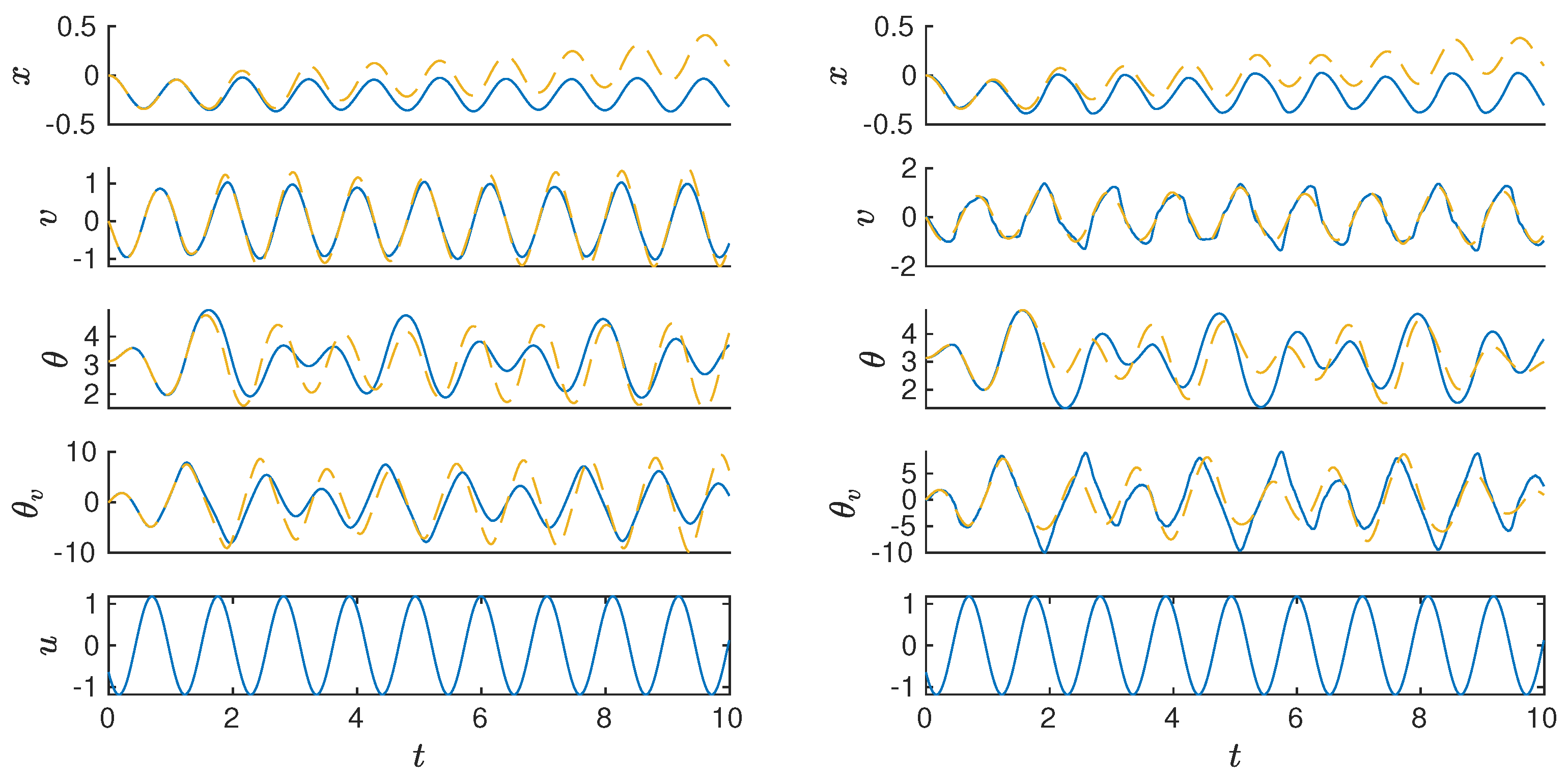
The EDMD algorithm gives a linear predictor equivalent to a discrete-time dynamical system. This predictor is suitable for the synthesis of controllers that drive the system to a desired state. The reliability of such a controller depends on the ability of the predictor to give accurate approximation of the dynamics for arbitrarily long time intervals. Therefore, for testing the strength of the algorithm, an additional test trajectory is considered where the simulation or experimental times are three times longer than the training and testing sets used for the computation and validation of the method. The result of evaluating the p-q-Trigonometric EDMD linear predictors on these additional long-term sets is depicted in Figure 9, where the mean absolute error for the approximation of the numerical simulation of the pendulum is 0.75 and the maximum absolute error is 6.05. For the experimental trajectories, the mean absolute error is 0.72 and the maximum absolute error is 7.31. These results show that, for these particular cases, the method is reliable enough for the prediction of the long term dynamics of the system.

5. Conclusions

This paper deals with extensions and improvements to the EDMD algorithm for special cases where there is an a priori knowledge of the behavior of a subset of state variables in terms of elemental function, such as trigonometric or logarithmic functions, among others. This expansion of the state, coupled with the use of p-q-quasi norms, gives an algorithmic advantage for the approximation of the dynamics of non-linear systems in a data-driven way. Although this approach improves the accuracy of the approximation, the expansion of the state has the risk of increasing the dimension of the set of observables necessary to perform the approximation. As a consequence, the algorithm can fall into the course of the dimensionality problem making solutions computationally unfeasible.

These embeddings represent an additional step for the formulation of observables that better suit a particular system, depending on the ability to select proper embeddings for the state variables. Consequently, they represent a contribution to the open problem of the proper selection of observables for the EDMD algorithm.

On the subject matter of observable selection, there is still the open question of the method to incorporate the knowledge of available models, in a similar fashion as traditional modeling and identification techniques. A combination of the two paradigms, the black box and solely data-driven methods, such as the EDMD, and the traditional identification techniques, has the potential of reducing the necessary set of observables further while also improving the accuracy even further.