Cyclic Control Optimization Algorithm for Stirling Engines

Abstract

The ideal Stirling cycle describes a specific way to operate an equilibrium Stirling engine. This cycle consists of two isothermal and two isochoric strokes. For non-equilibrium Stirling engines, which may feature various irreversibilities and whose dynamics is characterized by a set of coupled ordinary differential equations, a control strategy that is based on the ideal cycle will not necessarily yield the best performance—for example, it will not generally lead to maximum power. In this paper, we present a method to optimize the engine’s piston paths for different objectives; in particular, power and efficiency. Here, the focus is on an indirect iterative gradient algorithm that we use to solve the cyclic optimal control problem. The cyclic optimal control problem leads to a Hamiltonian system that features a symmetry between its state and costate subproblems. The symmetry manifests itself in the existence of mutually related attractive and repulsive limit cycles. Our algorithm exploits these limit cycles to solve the state and costate problems with periodic boundary conditions. A description of the algorithm is provided and it is explained how the control can be embedded in the system dynamics. Moreover, the optimization results obtained for an exemplary Stirling engine model are discussed. For this Stirling engine model, a comparison of the optimized piston paths against harmonic piston paths shows significant gains in both power and efficiency. At the maximum power point, the relative power gain due to the power-optimal control is ca. 28%, whereas the relative efficiency gain due to the efficiency-optimal control at the maximum efficiency point is ca. 10%.

1. Introduction

Stirling engines are closed-cycle regenerative heat engines that harness a temperature difference between two external heat baths. At the cost of taking entropy from the hot heat bath and disposing it to the cold heat bath, they generate mechanical work. This means that Stirling engines are very flexible regarding the possible technical representations of those two heat baths. Therefore, they can be applied in various scenarios. Some current example applications are power generation from burnable industrial waste gases [1], domestic combined heat and power generation [2], electro-thermal energy storage systems for renewable energies as an alternative to lithium-ion batteries [3], and low-maintenance power generation in remote regions with harsh climatic conditions [4], among others. If properly designed, Stirling engines can achieve high efficiency, durability, low-maintenance, and low-noise operation. Hence, they are considered to be one good candidate technology for enhancing the sustainability of power systems.

One certain ideal representation of the thermodynamic cycle performed in Stirling engines is commonly referred to as the ideal Stirling cycle. It consists of four distinct strokes (processes) that an enclosed working gas cyclically performs:

• Isothermal compression at $T_{\mathrm{ExL}}$
• Isochoric regenerative heating to $T_{\mathrm{ExH}}$
• Isothermal expansion at $T_{\mathrm{ExH}}$
• Isochoric regenerative cooling to $T_{\mathrm{ExL}}$

where $T_{\mathrm{ExH}}$ and $T_{\mathrm{ExL}}$ are the temperatures of the hot and cold heat bath, respectively. If those four ideal processes are repeated in the prescribed order, the cycle represents an ideal heat engine, operating with Carnot efficiency ${\eta }_{\mathrm{C}}=1-T_{\mathrm{ExL}}/T_{\mathrm{ExH}}$. In the two regenerative processes 4 and 2, heat needs to be stored and provided at a range of temperatures. The combined process is called regeneration, and is accomplished with help of a multi-temperature heat storage, referred to as a regenerator.

In real Stirling engines, the working gas is typically contained in two working spaces. One of them, the hot working space, is in thermal contact with the hot heat bath. The other one, the cold working space, is in thermal contact with the cold heat bath. The two working spaces’ volumes can be changed by moving pistons. As a result of those pistons’ movements, the working spaces exchange working gas through the regenerator, which is often implemented as a porous metal structure.

In contrast to the ideal Stirling cycle, in real Stirling engines, the four above-described strokes can typically not be clearly distinguished. This is due to several reasons. First of all, the engine’s piston movements (piston paths) usually do not exactly reproduce the two isochoric strokes. Moreover, the regenerator, as well as the hot and cold working spaces, have non-zero dead volumes. The most important reason, however, is connected to the fact that real engines are supposed to produce a finite amount of work in finite time, which is in contrast to the assumptions of equilibrium thermodynamics, and thus to the ideal Stirling cycle. Consequently, in real Stirling engines, various inevitable loss phenomena occur, for example, finite heat transfer between the working gas and the external heat baths or the regenerator matrix, pressure drop across the regenerator, and heat leaks through the engine’s internal components.

Correspondingly, real Stirling engines are non-equilibrium devices. Hence, piston paths aiming to emulate the ideal Stirling cycle’s four strokes would not necessarily yield best performance. The question of what piston paths yield best performance, for example, optimal net power, constitutes a cyclic optimal control problem.

In this paper we present an algorithm that can be used to solve such cyclic optimal control problems. It is an indirect iterative gradient algorithm and based on Optimal Control Theory. The algorithm starts with prescribing initial control functions determining the piston paths. These control functions are then gradually modified over the course of the iterations so as to gradually improve an objective and approach the optimal control. To determine the gradual shifts in every iteration, not only does the system of ordinary differential equations, describing the thermodynamics of the Stirling engine, need to be solved, but also a conjugate system of differential equations. For the efficient practical feasibility of this task, low numerical effort of the utilized thermodynamic model is crucial. In detailed models of Stirling engines, significant numerical effort is usually connected to the description of the regenerator. Therefore, here we will apply a Stirling engine model with a reduced-order endoreversible regenerator model that provides a proper tradeoff between accuracy and numerical effort for optimal control problems.

As indicated above, the core discrepancy between the ideal Stirling cycle and a real Stirling engine is that, in the former, all processes are quasi-static, and hence reversible, whereas the latter is required to produce a finite amount of work in finite time. Therefore, real Stirling engines are non-equilibrium devices that could by no means achieve the performance measures of the ideal cycle, such as Carnot efficiency. A non-equilibrium thermodynamics field that studies how constraints on time and rate influence the performance of such devices is Finite-Time Thermodynamics (FTT) [5,6]. FTT typically approaches this and related questions with variational principles and global—rather than local—descriptions of the irreversible systems considered [5].

Endoreversible Thermodynamics [7,8,9,10,11] can be regarded as a subfield of FTT that intends to provide a toolbox of model building blocks from which an FTT model can be constructed in a comprehensible way. The emphasis is placed on including the main loss phenomena, while keeping the model structure clear and minimizing mathematical complexity and numerical effort. The basic approach is to decompose the considered thermodynamic system into a network of reversible subsystems that are connected with each other through (ir)reversible interactions. That is, in its endoreversible representation, the original system’s irreversibilities are captured by the interactions, whereas for the reversible subsystems the known relations from equilibrium thermodynamics hold.

In the past, various endoreversible systems have been subject to investigations involving control optimizations. In particular, for heat engines, the piston trajectories can be optimized for objectives, such as power or efficiency. For example, such studies have been carried out for engines with Diesel [11,12,13,14] and Otto [15,16,17] cycles, light-driven engines [18,19,20], and Stirling engines [21,22,23].

The optimization approach used in the current study to optimize the Stirling engine differs from [21,22,23] in that a cyclic version of Optimal Control Theory is applied. Beyond Endoreversible Thermodynamics, this has been done by Craun and Bamieh [24] for an ideal beta-Stirling engine model with an actively controlled displacer. In [24], the heat transfer between the heat baths and the working gas was infinitely fast and regeneration was perfect. The pressure drop across the regenerator was thermodynamically neglected, but considered in terms of mechanical losses. As opposed to this, in the current study, an alpha-Stirling engine model with finite heat transfer between the heat baths and the working gas, an external heat leak, gas leakages and friction of the piston rings, and an irreversible regenerator is considered. Compared to the endoreversible regenerator models used in [22,23], the EEn-regenerator model [25] used in this study features a significantly higher degree of detail.

2. Stirling Engine Model

In this paper, our focus is on a cyclic control optimization algorithm that can be applied to various Stirling engine models, or models of other cyclically operating systems. Nevertheless, we here briefly introduce a Stirling engine model [25] that we will use to demonstrate the algorithm’s usage. In particular, we will present optimization results for this model in Section 5.

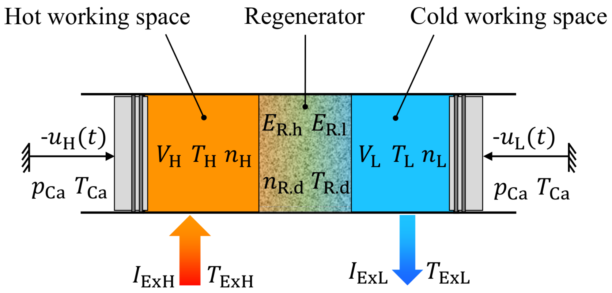
We consider an alpha-type Stirling engine as schematized in Figure 1, where the heat transfer between the external heat baths and the working gas is realized through the cylinders.

For the sake of simplicity, we assume a constant finite heat transfer coefficient. Further irreversibilities result from an external heat leak between the heat baths, gas leakage of the piston rings, friction of the pistons, pressure drop across the regenerator, and thermal mixing at the interfaces of the regenerator and the working spaces.

The regenerator is described with the reduced-order endoreversible EEn-regenerator model, developed in [25]. Essentially, this is based on the assumptions that the spatial temperature distribution inside the regenerator is linear and that the temperature difference between the gas and matrix is small. Aside from external irreversibilities that automatically occur due to thermal mixing in the regenerator’s interactions with the working spaces, internal irreversibilities can be included via entropy source terms in the EEn-regenerator model. In the current study, the irreversibility due to the pressure drop across the regenerator is accounted for by such an entropy source term.

The Stirling engine performance measures that are to be optimized in this study are power and efficiency. The power, or net power output, is defined as

$$\begin{array}{c}\hfill P=\frac{W}{\tau },\end{array}$$

(1)

with the fixed cycle time $\tau$ and the net cycle work

$$\begin{array}{c}\hfill W={\int }_0^{\tau }\left(p_{\mathrm{H}}{\dot{V}}_{\mathrm{H}}+p_{\mathrm{L}}{\dot{V}}_{\mathrm{L}}\right)-\gamma \left({\dot{V}}_{\mathrm{H}}^2+{\dot{V}}_{\mathrm{L}}^2\right)\mathrm{d}t,\end{array}$$

(2)

where $V_i$ and $p_i$ are the volume and pressure of the working spaces $i\in \left\{\mathrm{H},\mathrm{L}\right\}$ and $\gamma$ is the friction coefficient of the pistons. Then, the efficiency is

$$\begin{array}{c}\hfill \eta =\frac{{\int }_0^{\tau }\left(p_{\mathrm{H}}{\dot{V}}_{\mathrm{H}}+p_{\mathrm{L}}{\dot{V}}_{\mathrm{L}}\right)-\gamma \left({\dot{V}}_{\mathrm{H}}^2+{\dot{V}}_{\mathrm{L}}^2\right)\mathrm{d}t}{{\int }_0^{\tau }{I}_{\mathrm{H},\mathrm{ExH}}+K_{\mathrm{Ex}}\left(T_{\mathrm{ExH}}-T_{\mathrm{ExL}}\right)\mathrm{d}t},\end{array}$$

(3)

where $I_{\mathrm{H},\mathrm{ExH}}$ is the instantaneous heat flux to the hot working space and $K_{\mathrm{Ex}}$ ($T_{\mathrm{ExH}}-T_{\mathrm{ExL}}$) corresponds to an external heat leak. We here use the same transfer laws and parameter values as in [25], for example, the heat bath temperatures are defined as $T_{\mathrm{ExH}}=500$ K and $T_{\mathrm{ExL}}=300$ K. Solely for the heat conductance of the external heat leak, we chose a different parameter value: $K_{\mathrm{Ex}}=5$ W/K.

This Stirling engine model has ten state variables, which are the working spaces’ volumes $V_i$, temperatures $T_i$, and particle numbers $n_i$ with $i\in$ {H,L}, the energies $E_{\mathrm{R}.\mathrm{h}}$ and $E_{\mathrm{R}.\mathrm{l}}$ of the hot and cold halves of the regenerator matrix as well as the particle number $n_{\mathrm{R}.\mathrm{d}}$ and temperature $T_{\mathrm{R}.\mathrm{d}}$ of the gas inside the regenerator dead space.

The state variables of this Stirling engine model can be arranged in a state vector $\mathit{x}$ and the state dynamics can be expressed in terms of $\dot{\mathit{x}}=\mathit{f}(\mathit{x},\mathit{u})$. Here, $\mathit{f}(\mathit{x},\mathit{u})$ is a vector-valued function that depends on the state vector $\mathit{x}$ and a control vector $\mathit{u}$. In our Stirling engine model we define the control vector $\mathit{u}$ in terms of an explicitly time-dependent, $\tau$-periodic control function $\mathit{u}\left(t\right)$, which has the entries $u_{\mathrm{H}}\left(t\right)$ and $u_{\mathrm{L}}\left(t\right)$. Each of those two sub-functions determines the dynamics of one working volume, as indicated in Figure 1. An essential requirement that we raise is that the state dynamics $\dot{\mathit{x}}=\mathit{f}(\mathit{x},\mathit{u}\left(t\right))$ features a limit cycle with regard to all state variables, which will be necessary for the applicability of the optimization algorithm. Therefore, care must be taken regarding the embedding of the control in the system dynamics, which will be explained in Section 4.

3. Cyclic Optimal Control Problem

Optimal Control Theory provides a framework for the dynamic (or indirect) optimization of dynamical systems, such as the above-described Stirling engine model. The type of optimal control problem considered in this work can be formulated as: find an unconstrained, smooth, $\tau$-periodic control function $\mathit{u}\left(t\right)$ that maximizes the objective functional

$$\begin{array}{c}\hfill J={\int }_0^{\tau }\zeta (\mathit{x},\mathit{u}\left(t\right))\mathrm{d}t\end{array}$$

(4)

subject to the constraint

$$\begin{array}{c}\hfill \dot{\mathit{x}}=\mathit{f}(\mathit{x},\mathit{u}\left(t\right))\end{array}$$

(5)

for a fixed period $\tau$. Here, $\mathit{x}$ is the state vector of the system. The dynamics of the system is determined by the ordinary differential Equation (5) and is influenced by the vector-valued, explicitly time-dependent, $\tau$-periodic control function $\mathit{u}\left(t\right)$.

For the formulation of necessary conditions of optimality, a Hamilton function H is defined as [26,27]

$$\begin{array}{c}\hfill H(\mathit{x},\mathit{u},\mathit{\lambda }):=\zeta (\mathit{x},\mathit{u})+{\mathit{\lambda }}^T\mathit{f}(\mathit{x},\mathit{u})\end{array}$$

(6)

with an adjoint vector $\mathit{\lambda }$, which varies over time and will henceforth also be called a costate vector. As we will see later, there exists an interesting symmetry between the dynamics of the state vector $\mathit{x}$ and the costate vector $\mathit{\lambda }$. The first order necessary conditions for the control $\mathit{u}$ with the optimal value are [26,27]

$$\begin{array}{c}\hfill \dot{\mathit{x}}={\nabla }_{\mathit{\lambda }}H(\mathit{x},\mathit{u},\mathit{\lambda }),\end{array}$$

(7)

$$\begin{array}{c}\hfill \dot{\mathit{\lambda }}={\nabla }_{\mathit{x}}H(\mathit{x},\mathit{u},\mathit{\lambda }),\end{array}$$

(8)

$$\begin{array}{c}\hfill \mathbf{0}={\nabla }_{\mathit{u}}H(\mathit{x},\mathit{u},\mathit{\lambda }),\end{array}$$

(9)

combined with the respective transversality conditions that specify the boundary conditions for the state and costate dynamics from Equations (7) and (8), respectively. In the case of the optimal cyclic regime, as valid for the stationary operational state of a cyclically operating engine, these boundary conditions are [27]

$$\begin{array}{c}\hfill {\mathit{x}|}_{\tau }{=\mathit{x}|}_0,\end{array}$$

(10)

$$\begin{array}{c}\hfill {\mathit{\lambda }|}_{\tau }{=\mathit{\lambda }|}_0.\end{array}$$

(11)

The notation ${\mathit{x}|}_t$ refers to the value of $\mathit{x}$ at time t, while it does not indicate explicit time dependence. These boundary conditions do not render the problem overdetermined, since the initial and final values are not quantified, but only required to be equal.

In this way, the global dynamic optimization problem from Equation (4) with the constraint Equation (5) is turned into the continuous set of local (static) optimization problems from Equation (9) with the constraints Equations (7) and (8). This means that $H(\mathit{x},\mathit{u},\mathit{\lambda })$ must be locally maximized for all $t\in \left[0,\tau \right)$ with respect to $\mathit{u}$. For the optimal solution ${\mathit{x}}^{\ast }$, ${\mathit{u}}^{\ast }$, ${\mathit{\lambda }}^{\ast }$ of the considered kind of cyclic optimization problem, without explicit time dependence of $\zeta (\mathit{x},\mathit{u})$, the temporal value of the Hamilton function $H^{\ast }$ will then be constant [26,27].

3.1. Maximum Power

In the case of the optimization being performed for the objective functional, which is the cycle-averaged net power output P, as defined in Equation (1), the definition of the path target function $\zeta (\mathit{x},\mathit{u})$ for Equations (4) and (6) is straightforward:

$$\begin{array}{c}\hfill {\zeta }_{\mathrm{W}}(\mathit{x},\mathit{u}):=\left(p_{\mathrm{H}}{\dot{V}}_{\mathrm{H}}+p_{\mathrm{L}}{\dot{V}}_{\mathrm{L}}\right)-\gamma \left({\dot{V}}_{\mathrm{H}}^2+{\dot{V}}_{\mathrm{L}}^2\right),\end{array}$$

(12)

which is simply the instantaneous power output. Since the optimization is performed for fixed cycle time $\tau$, maximum power corresponds to maximum work. Hence, a prefactor of $1/\tau$ can be disregarded here.

3.2. Maximum Efficiency

In the case of the optimization being performed for the objective of efficiency $\eta$, as defined in Equation (3), the definition of $\zeta (\mathit{x},\mathit{u})$ is slightly more involved. This is because the definition of the efficiency corresponds to a ratio of two functionals (integrals) which need to be separately evaluated before calculating their ratio. This can be seen in Equation (3) and is in contrast to the structure of Equation (4). In order to resolve this discrepancy, we investigate how variations in the cycle work W and the heat $Q_{\mathrm{H}}:={\int }_0^{\tau }{I}_{\mathrm{H},\mathrm{ExH}}+K_{\mathrm{Ex}}\left(T_{\mathrm{ExH}}-T_{\mathrm{ExL}}\right)\mathrm{d}t$ translate to the first variation of the efficiency:

$$\begin{array}{c}\hfill \delta \eta =\delta \left(\frac{W}{Q_{\mathrm{H}}}\right)=\frac{\partial \eta }{\partial W}\delta W+\frac{\partial \eta }{\partial Q_{\mathrm{H}}}\delta Q_{\mathrm{H}}=\frac{1}{Q_{\mathrm{H}}}\delta W-\frac{W}{Q_{\mathrm{H}}^2}\delta Q_{\mathrm{H}}.\end{array}$$

(13)

This means that the problem of optimizing the efficiency can be morphed into an equivalent optimization problem of the weighted sum ${\lambda }_{\mathrm{W}}W+{\lambda }_{\mathrm{QH}}{Q}_{\mathrm{H}}$ with the weights being defined according to the partial derivatives:

$$\begin{array}{c}\hfill {\lambda }_{\mathrm{W}}=\partial \eta /\partial W=1/Q_{\mathrm{H}}\mathrm{and}{\lambda }_{\mathrm{QH}}=\partial \eta /\partial Q_{\mathrm{H}}=-W/Q_{\mathrm{H}}^2.\end{array}$$

(14)

Within these weights, W and $Q_{\mathrm{H}}$ are the results obtained for a specific prescribed $\tau$-periodic control function ${\mathit{u}}^{†}\left(t\right)$ for which, at a given time t, the values of the control and state vectors are $\mathit{u}\approx {\mathit{u}}^{†}\left(t\right)$ and $\mathit{x}\approx {\mathit{x}}^{†}\left(t\right)$. Here, ${\mathit{x}}^{†}\left(t\right)$ is the periodic solution of the state dynamics for ${\mathit{u}}^{†}\left(t\right)$. Based on this, we can now define the path target function for maximizing the efficiency:

$$\begin{array}{c}\hfill {\zeta }_{\eta }(\mathit{x},\mathit{u}):=\frac{W}{Q_{\mathrm{H}}\tau }+\frac{1}{Q_{\mathrm{H}}}{\zeta }_{\mathrm{W}}(\mathit{x},\mathit{u})-\frac{W}{Q_{\mathrm{H}}^2}{I}_{\mathrm{H},\mathrm{ExH}}(\mathit{x},\mathit{u}).\end{array}$$

(15)

Here, W and $Q_{\mathrm{H}}$ are again the results obtained for a $\tau$-periodic control function ${\mathit{u}}^{†}\left(t\right)$ with the above-described closeness requirements for the instantaneous values of $\mathit{x}$ and $\mathit{u}$. In a strict sense, the path target function ${\zeta }_{\eta }(\mathit{x},\mathit{u})$ is therefore also a functional of ${\mathit{u}}^{†}\left(t\right)$ and ${\mathit{x}}^{†}\left(t\right)$, that is: ${\zeta }_{\eta }(\mathit{x},\mathit{u})={\zeta }_{\eta }{[\mathit{x}}^{†}(·),{\mathit{u}}^{†}(·)](\mathit{x},\mathit{u})$ because $W=W[{\mathit{x}}^{†}(·),{\mathit{u}}^{†}(·)]$ and $Q_{\mathrm{H}}=Q_{\mathrm{H}}[{\mathit{x}}^{†}(·),{\mathit{u}}^{†}(·)]$. If the closeness requirement of $\mathit{x}$ and $\mathit{u}$, regarding ${\mathit{u}}^{†}\left(t\right)$ is valid for all t, the second and third terms in Equation (15) will (approximately) cancel upon integration from 0 to $\tau$. Therefore, the first term was added here to ensure that ${\int }_0^{\tau }{\zeta }_{\eta }(\mathit{x},\mathit{u})\mathrm{d}t$ does actually represent $\eta$. This first term does, in fact, not influence the optimization problem from Equation (7) to Equation (11), since it does not depend on the instantaneous values of $\mathit{x}$ and $\mathit{u}$.

3.3. Penalty Function

The cyclic optimal control problem introduced so far does not contain inequality constraints for the state $\mathit{x}$ or the control $\mathit{u}$. However, we can introduce inequality constraints for $\mathit{x}$ and $\mathit{u}$ by means of a penalty function. In particular, we will use such a penalty function to introduce lower and upper bounds for the Stirling engine’s working volumes:

$$\begin{array}{c}\hfill {\zeta }_{\mathrm{penalty}}(\mathit{x},\mathit{u}):=-v_0\left(e^{v_1\frac{V_{\mathrm{H},\min }-V_{\mathrm{H}}}{V_{\mathrm{H},\mathrm{sw}}}}+e^{v_1\frac{V_{\mathrm{H}}-V_{\mathrm{H},\max }}{V_{\mathrm{H},\mathrm{sw}}}}+e^{v_1\frac{V_{\mathrm{L},\min }-V_{\mathrm{L}}}{V_{\mathrm{L},\mathrm{sw}}}}+e^{v_1\frac{V_{\mathrm{L}}-V_{\mathrm{L},\max }}{V_{\mathrm{L},\mathrm{sw}}}}\right)\end{array}$$

(16)

where the working volumes $V_i$ are contained in $\mathit{x}$, $v_0=1$ W and $v_1=500$ are penalty factors, $V_{i,\mathrm{sw}}=V_{i,\max }-V_{i,\min }$ refers to the admissible swept volumes and $V_{i,\max }$ and $V_{i,\min }$ are the maximum and minimum admissible working volumes with $i\in \left\{\mathrm{H},\mathrm{L}\right\}$.

Accordingly, in the case of optimizing the Stirling engine’s piston paths for maximum power, the overall path target function is defined as

$$\begin{array}{c}\hfill \zeta (\mathit{x},\mathit{u}):={\zeta }_{\mathrm{W}}(\mathit{x},\mathit{u})+{\zeta }_{\mathrm{penalty}}(\mathit{x},\mathit{u}),\end{array}$$

(17)

whereas in case of the optimization for maximum efficiency, it is defined as

$$\begin{array}{c}\hfill \zeta (\mathit{x},\mathit{u}):={\zeta }_{\eta }(\mathit{x},\mathit{u})+{\zeta }_{\mathrm{penalty}}(\mathit{x},\mathit{u}).\end{array}$$

(18)

4. Optimization Algorithm

The indirect iterative gradient method described in the following was inspired by a contribution of Craun and Bamieh [24,28], who solved an optimal control problem of a modified beta-Stirling engine using an ideal thermodynamic model, namely the Schmidt model. Similar methods have earlier been used, for example, by Horn and Lin [29], Kowler and Kadlec [30], as well as Noorden et al. [31] for other applications. The method presented in this paper differs from the aforementioned ones in the means by which the periodic solutions of the state and costate equations are obtained. A pseudocode representation of the cyclic control optimization algorithm is shown in Algorithm 1.

Algorithm 1 Cyclic optimal control algorithm.

1: //############ Basic functions of the control problem ############ 2: define $\mathit{f}(\mathit{x},\mathit{u})\{$                           // RHS of state dynamics 3:    return temporal rate of state vector; 4: $\};$ 5: define $\zeta (\mathit{x},\mathit{u},\overline{\mathit{a}})\{$                        // Path cost function, $\overline{\mathit{a}}$ may contain W and $Q_{\mathrm{H}}$ 6:    return path cost value; 7: $\};$ 8: define $H(\mathit{x},\mathit{u},\mathit{\lambda },\overline{\mathit{a}})\{$                   // Hamilton function 9:    return $\zeta (\mathit{x},\mathit{u},\overline{\mathit{a}})+{\mathit{\lambda }}^T\mathit{f}(\mathit{x},\mathit{u});$ 10: $\};$ 11: define $-{\nabla }_{\mathit{x}}^{\mathrm{app}}H(\mathit{x},\mathit{u},\mathit{\lambda },\overline{\mathit{a}})\{$            // Approximation of RHS of costate dynamics 12:    declare $\epsilon =\mathrm{small}\mathrm{number};$ 13:    declare ${\widehat{\mathit{e}}}_m=\mathrm{unit}\mathrm{vector}\mathrm{of}{m}^{\mathrm{th}}\mathrm{state}\mathrm{component};$ 14:    return ${\sum }_m-{\widehat{\mathit{e}}}_m\left(H(\mathit{x}+\epsilon {\widehat{\mathit{e}}}_m,\mathit{u},\mathit{\lambda },\overline{\mathit{a}})-H(\mathit{x},\mathit{u},\mathit{\lambda },\overline{\mathit{a}})\right)/\epsilon ;$ 15: $\};$ 16: define ${\nabla }_{\mathit{u}}^{\mathrm{app}}H(\mathit{x},\mathit{u},\mathit{\lambda },\overline{\mathit{a}})\{$            // Approximation of control gradient function 17:    declare $\epsilon =\mathrm{small}\mathrm{number};$ 18:    declare ${\widehat{\mathit{e}}}_m=\mathrm{unit}\mathrm{vector}\mathrm{of}{m}^{\mathrm{th}}\mathrm{control}\mathrm{component};$ 19:    return ${\sum }_m{\widehat{\mathit{e}}}_m\left(H(\mathit{x},\mathit{u}+\epsilon {\widehat{\mathit{e}}}_m,\mathit{\lambda },\overline{\mathit{a}})-H(\mathit{x},\mathit{u}-\epsilon {\widehat{\mathit{e}}}_m,\mathit{\lambda },\overline{\mathit{a}})\right)/\left(2\epsilon \right);$ 20: $\};$ 21: //########## Declare control, state, and costate functions ########### 22: declare $\tau =\mathrm{cycle}\mathrm{time};$                // Define cycle time 23: declare $\mathit{u}\left(t\right)$ with $t\in \left[0,\tau \right);$          // Control vector function 24: declare $\mathit{x}\left(t\right)$ with $t\in \left[0,\tau \right);$          // State vector function 25: declare $\mathit{\lambda }\left(t\right)$ with $t\in \left[0,\tau \right);$          // Costate vector function 26: initialize $\mathit{u}\left(t\right)$ with smooth guess of optimal control vector function; 27: initialize $\mathit{x}\left(0\right)$ with arbitrary admissible values; 28: initialize $\mathit{\lambda }\left(0\right)=\mathbf{0};$ 29: //############ Iterative optimization of the control ############# 30: for $\left(n=0;n<\mathrm{large}\mathrm{number};n=n+1\right)\{$ 31:    while($\epsilon >$ small number){                                    // Solve state dynamics 32:       for($t=0;t<\tau ;t+=\Delta t$)   $\{ \mathit{x}(t+\Delta t)=\mathit{x}(t)+\mathit{f}(\mathit{x}\left(t\right),\mathit{u}\left(t\right))\Delta t; \}$   33:       $\epsilon =\left|\right|\mathit{x}\left(\tau \right)-\mathit{x}\left(0\right)\left|\right|;$ 34:       $\mathit{x}\left(0\right)=\mathit{x}\left(\tau \right);$ 35:     $\}$ 36:    declare $\mathit{a}\left(t\right)=$ some_function($\mathit{x}\left(t\right)$,$\mathit{u}\left(t\right)$) for $t\in \left[0,\tau \right);$ // Auxiliary vector function 37:    declare $\overline{\mathit{a}}=$ cycle average of $\mathit{a}\left(t\right)$ for $t\in \left[0,\tau \right);$          // Auxiliary vector cycle average 38:    while($\epsilon >$ small number){                                     // Solve costate dynamics 39:       $\mathit{\lambda }\left(\tau \right)=\mathit{\lambda }\left(0\right);$ 40:       for($t=\tau ;t>0;t-=\Delta t$)   $\{ \mathit{\lambda }(t-\Delta t)=\mathit{\lambda }\left(t\right)-{\nabla }_{\mathit{x}}^{\mathrm{app}}H(\mathit{x}\left(t\right),\mathit{u}\left(t\right),\mathit{\lambda }\left(t\right),\overline{\mathit{a}})\Delta t; \}$   41:       $\epsilon =\left|\right|\mathit{\lambda }\left(\tau \right)-\mathit{\lambda }\left(0\right)\left|\right|;$ 42:     $\}$ 43:    declare $\mathbf{s}\left(t\right)={\nabla }_{\mathit{u}}^{\mathrm{app}}H(\mathit{x}\left(t\right),\mathit{u}\left(t\right),\mathit{\lambda }\left(t\right))$ for $t\in \left[0,\tau \right);$    // Define search direction 44:    smooth $\mathbf{s}\left(t\right)$ in the periodic domain $t\in \left[0,\tau \right);$           // Smooth search direction 45:    declare $\mathsf{\Lambda }=\mathrm{small}\mathrm{number};$                                    // Step-size factor 46:    update $\mathit{u}\left(t\right)=\mathit{u}\left(t\right)+\mathsf{\Lambda }\mathbf{s}\left(t\right)$ for $t\in \left[0,\tau \right);$                 // Shift control 47:    smooth $\mathit{u}\left(t\right)$ in the periodic domain $t\in \left[0,\tau \right);$           // Smooth control 48:     $\}$

In the first section, between lines 1 and 20, the basic function definitions are made. First, the right-hand side (RHS) of the state dynamics is defined as a vector function $\mathit{f}(\mathit{x},\mathit{u})$. Afterwards, the path cost function $\zeta (\mathit{x},\mathit{u},\overline{\mathit{a}})$ that is to be maximized in terms of the objective functional from Equation (4) is defined. Here, the argument $\overline{\mathit{a}}$ may, for example, contain the cycle work W and heat $Q_{\mathrm{H}}$, as required in Equation (15). Then, based on the definition of the Hamilton function $H(\mathit{x},\mathit{u},\mathit{\lambda },\overline{\mathit{a}})$ from lines 8 to 10, the right-hand side of the costate dynamics $-{\nabla }_{\mathit{x}}^{\mathrm{app}}H(\mathit{x},\mathit{u},\mathit{\lambda },\overline{\mathit{a}})$ is defined in terms of an approximation:

$$\begin{array}{c}\hfill -\frac{\partial H(\mathit{x},\mathit{u},\mathit{\lambda },\overline{\mathit{a}})}{\partial x_m}\approx -\frac{H(\mathit{x}+\epsilon {\widehat{\mathit{e}}}_m,\mathit{u},\mathit{\lambda },\overline{\mathit{a}})-H(\mathit{x},\mathit{u},\mathit{\lambda },\overline{\mathit{a}})}{\epsilon }\end{array}$$

(19)

where $x_m$ is the mth state component, ${\widehat{\mathit{e}}}_m$ is the corresponding unit vector and $\epsilon$ is a sufficiently small difference. For simple systems, it is reasonable to derive this right-hand side in terms of algebraic expressions. However, for involved systems it can be much more practical to do this by numerical partial differentiation as, for example, according to Equation (19). Note that for systems with discontinuous dynamics additional care must be taken here in order to make sure that the derivatives are properly approximated in the vicinity of the discontinuity. Similarly to $-{\nabla }_{\mathit{x}}^{\mathrm{app}}H(\mathit{x},\mathit{u},\mathit{\lambda },\overline{\mathit{a}})$, the vector ${\nabla }_{\mathit{u}}^{\mathrm{app}}H(\mathit{x},\mathit{u},\mathit{\lambda },\overline{\mathit{a}})$ of partial derivatives of the Hamilton function with respect to the control is defined from lines 16 to 20. Here, the following approximation is used:

$$\begin{array}{c}\hfill \frac{\partial H(\mathit{x},\mathit{u},\mathit{\lambda },\overline{\mathit{a}})}{\partial u_m}\approx \frac{H(\mathit{x},\mathit{u}+\epsilon {\widehat{\mathit{e}}}_m,\mathit{\lambda },\overline{\mathit{a}})-H(\mathit{x},\mathit{u}-\epsilon {\widehat{\mathit{e}}}_m,\mathit{\lambda },\overline{\mathit{a}})}{2\epsilon }\end{array}$$

(20)

where $u_m$ is the mth control component, ${\widehat{\mathit{e}}}_m$ is the corresponding unit vector and $\epsilon$ is, again, a sufficiently small difference.

In the second section between lines 21 and 28, the most relevant variables are declared and initialized. These are the control vector function $\mathit{u}\left(t\right)$, the state vector function $\mathit{x}\left(t\right)$, and the costate vector function $\mathit{\lambda }\left(t\right)$. They are defined in the time domain $\left[0,\tau \right)$ and may be implemented as vectors of arrays, where the array lengths correspond to the number of time steps per period. That means that the values of $\mathit{u}$, $\mathit{x}$, and $\mathit{\lambda }$ are saved at every time step in the periodic domain. The control vector function $\mathit{u}\left(t\right)$ is initialized with a smooth $\tau$-periodic guess of the optimal control. Moreover, $\mathit{x}\left(0\right)$ is set to arbitrary but physically admissible values, whereas $\mathit{\lambda }\left(0\right)$ is set to $\mathbf{0}$.

The iterative control optimization itself is described in the third section between lines 29 and 48. This starts at iteration $n=0$ with the initial guess of the smooth $\tau$-periodic control function ${\mathit{u}}^{\left(0\right)}\left(t\right)$, and the previously defined state and costate initial values ${\mathit{x}}^{\left(0\right)}\left(0\right)$ and ${\mathit{\lambda }}^{\left(0\right)}\left(0\right)$, respectively. Here, the bracketed superscript identifies the iteration n of the for-loop from lines 30 to 48. Since the control is predefined, the state and costate problem can be solved separately. The steps to obtain the subsequent iteration ${\mathit{u}}^{(n+1)}\left(t\right)$, according to Algorithm 1, can be summarized in simplified terms:

0.

If $n=0$, set ${\mathit{x}}^{\left(0\right)}\left(0\right)$ to arbitrary physically admissible values and ${\mathit{\lambda }}^{\left(0\right)}\left(0\right):=\mathbf{0}$. Otherwise, set ${\mathit{x}}^{\left(n\right)}\left(0\right):={\mathit{x}}^{(n-1)}\left(\tau \right)$ and ${\mathit{\lambda }}^{\left(n\right)}\left(0\right):={\mathit{\lambda }}^{(n-1)}\left(\tau \right)$.

1.

For given ${\mathit{u}}^{\left(n\right)}\left(t\right)$: Solve

$$\begin{array}{c}\hfill {\dot{\mathit{x}}}^{\left(n\right)}\left(t\right)=\mathit{f}({\mathit{x}}^{\left(n\right)}\left(t\right),{\mathit{u}}^{\left(n\right)}\left(t\right))\end{array}$$

by temporal forward integration in the periodic domain until the cyclic equilibrium is reached. Save auxiliary quantities, such as the cycle work W and the heat $Q_{\mathrm{H}}$ in ${\overline{\mathit{a}}}^{\left(n\right)}$. (Algorithm 1, lines 31 to 37: example with Euler method.)

2.

For given ${\mathit{u}}^{\left(n\right)}\left(t\right)$, ${\mathit{x}}^{\left(n\right)}\left(t\right)$, ${\overline{\mathit{a}}}^{\left(n\right)}$: Solve

$$\begin{array}{c}\hfill {\dot{\mathit{\lambda }}}^{\left(n\right)}\left(t\right)=-{\nabla }_{\mathit{x}}H({\mathit{x}}^{\left(n\right)}\left(t\right),{\mathit{u}}^{\left(n\right)}\left(t\right),{\mathit{\lambda }}^{\left(n\right)}\left(t\right),{\overline{\mathit{a}}}^{\left(n\right)})\end{array}$$

by temporal backward integration in the periodic domain until the cyclic equilibrium is reached. (Algorithm 1, lines 38 to 42: example with Euler method.)

3.

Calculate the search direction (See Algorithm 1, line 43.)

$$\begin{array}{c}\hfill {\mathbf{s}}^{\left(n\right)}\left(t\right):={\nabla }_{\mathit{u}}H({\mathit{x}}^{\left(n\right)}\left(t\right),{\mathit{u}}^{\left(n\right)}\left(t\right),{\mathit{\lambda }}^{\left(n\right)}\left(t\right)).\end{array}$$

4.

Calculate the next control vector function

$$\begin{array}{c}\hfill {\mathit{u}}^{(n+1)}\left(t\right):={\mathit{u}}^{\left(n\right)}\left(t\right)+\mathsf{\Lambda }{\mathbf{s}}^{\left(n\right)}\left(t\right)\end{array}$$

with a sufficiently small positive step-size factor $\mathsf{\Lambda }$. (Algorithm 1, line 46.)

These five steps are repeated for increasing n until ${\mathit{u}}^{\left(n\right)}\left(t\right)$ has converged to the optimal control. This can, for example, be checked with the below indicators which should both approach a numerical zero:

$$\begin{array}{c}\hfill C_{\nabla }^{\left(n\right)}:={\int }_0^{\tau }{\left({\nabla }_{\mathit{u}}H({\mathit{x}}^{\left(n\right)}\left(t\right),{\mathit{u}}^{\left(n\right)}\left(t\right),{\mathit{\lambda }}^{\left(n\right)}\left(t\right))\right)}^2\mathrm{d}t,\end{array}$$

(21)

$$\begin{array}{c}\hfill C_{\mathrm{H}}^{\left(n\right)}:=\underset{t}{\max }H({\mathit{x}}^{\left(n\right)}\left(t\right),{\mathit{u}}^{\left(n\right)}\left(t\right),{\mathit{\lambda }}^{\left(n\right)}\left(t\right))-\underset{t}{\min }H({\mathit{x}}^{\left(n\right)}\left(t\right),{\mathit{u}}^{\left(n\right)}\left(t\right),{\mathit{\lambda }}^{\left(n\right)}\left(t\right)).\end{array}$$

(22)

4.1. Exploiting Limit Cycles

The dynamic systems considered here are required to posses a limit cycle. This means that, given a proper periodic control function, the systems feature a closed state trajectory ${\mathit{x}}_{\infty }\left(t\right)$ in the state space, which is attractive. Here, the subscript ∞ refers to this limit cycle. If the state dynamics is integrated forward in time starting from $t=0$ with a proper initial value ${\mathit{x}|}_0$ in the vicinity of ${\mathit{x}}_{\infty }\left(0\right)$, then ${\mathit{x}|}_t\to {\mathit{x}}_{\infty }\left(t\right)$ for $t\to \infty$. This is a property of many dissipative systems, and it is directly made use of in the first step (Algorithm 1, lines 31 to 35) for finding the periodic solution of the state vector.

Numerical studies of optimal control problems carried out in the context of this work show an interesting type of symmetry in that the costate dynamics then features a limit cycle, too, for prescribed $\mathit{u}\left(t\right)$ and ${\mathit{x}|}_t:={\mathit{x}}_{\infty }\left(t\right)$. However, the respective closed trajectory ${\mathit{\lambda }}_{\infty }\left(t\right)$ is repulsive when the costate dynamics is considered forward in time, and becomes attractive in the reversed time direction: ${\mathit{\lambda }|}_t\to {\mathit{\lambda }}_{\infty }\left(t\right)$ for $t\to \infty$.Such a relation is not surprising, as the overall Hamiltonian system is conservative and the expansive costate dynamics compensates for the contractive state dynamics. Therefore, in the second step (Algorithm 1, line 38 to 42), the temporal direction of integration is reversed to obtain the periodic solution of the costate vector.

The correspondingly enhanced stability of the costate problem under temporal backward integration can also be exploited without directly making use of the limit-cycle property for obtaining the periodic solution, but for solving boundary value problems, for example, see [26,31].

4.2. Proper Embedding of the Control

Note that the way in which the control is embedded in the system’s state dynamics, can influence the existence of these limit cycles in the state and costate problems. In the Stirling engine optimization problem, considered in this paper, our goal is to optimize the piston paths. Hence, we chose to structure the system dynamics in such a way that the control function determines the temporal evolution of the working space volumes $V_i$ with $i\in \left\{\mathrm{H},\mathrm{L}\right\}$. A rather obvious choice for embedding the control $u_i\left(t\right)$ would be:

$$\begin{array}{c}\hfill \dot{V_i}=u_i\left(t\right).\end{array}$$

(23)

For an explicitly time-dependent, $\tau$-periodic control $u_i\left(t\right)$ that has an average value ${\int }_0^{\tau }{u}_i\left(t\right)\mathrm{d}t=0$, the resulting volumes $V_i$ will be $\tau$-periodic. However, this dynamics does not feature a limit cycle: The solution of $V_i{|}_t$ will even for t being large integer multiples of $\tau$ remain equal to the initial value $V_i{|}_0$ from which integration was started. This will translate to the costate problem, so that the solution algorithm from above will, in general, not converge without further manipulation of the optimization problem.

A proper choice for embedding the control in the system’s state dynamics that leads to the existence of a limit cycle for a continuous $\tau$-periodic $u_i\left(t\right)$ is:

$$\begin{array}{c}\hfill \dot{V_i}=\frac{\nu }{\tau }\left(u_i\left(t\right)-V_i\right)\end{array}$$

(24)

with a sufficiently large number $\nu$. This dynamics is similar to that of an overdamped mass-spring-damper system, where the spring support moves according to $u_i\left(t\right)$. If $\nu \to \infty$ then $V_i{|}_t\to u_i\left(t\right)$ for $t\to \infty$, independent of the initial value $V_i{|}_0$. That is, for $\nu \to \infty$, the control vector function $\mathit{u}\left(t\right)$ represents the limit cycle ${\mathit{V}}_{\infty }\left(t\right)$ of the volumes.

5. Results

The previously described optimization algorithm was applied to the exemplary alpha-Stirling engine model presented in Section 2 to optimize the control (piston paths) regarding both power and efficiency. The optimizations were performed for varying cycle time $\tau$, or correspondingly varying engine speed $1/\tau$. With help of the penalty function from Equation (16), the working volumes were restricted to an approximate range from 100 cm${}^3$ to 1100 cm${}^3$. The initial control, from which the optimizations were started, corresponds to harmonic piston paths exploiting the complete admissible working volume range and featuring a phase shift of ${90}^{\circ }$. This harmonic control will, in the following, also be used as a benchmark.

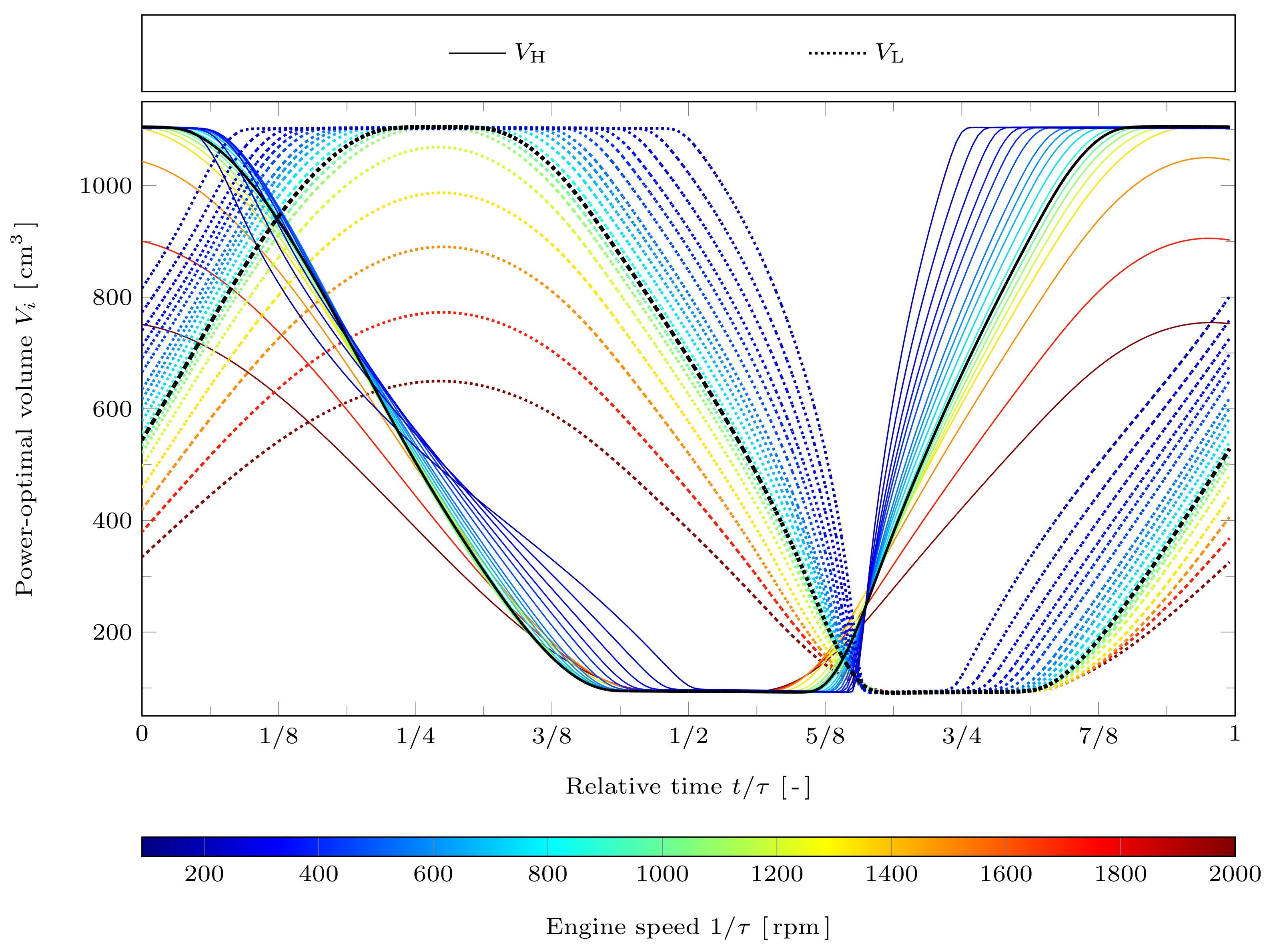
In Figure 2, the Stirling engine’s power-optimal working volume trajectories are shown for different engine speeds.

It can be seen that the power-optimal volume trajectories significantly deviate from harmonic shapes. At low engine speeds, it is favorable to let the pistons rest in their extreme positions for about half the cycle time. This feature is less pronounced at higher engine speeds. Above ca. 1100 rpm and ca. 1300 rpm the power-optimal working volume trajectories detach from the maximum volume bounds, as can be seen in Figure 2 at $t/\tau \approx 1/4$ and $t/\tau \approx 1$, respectively. At the highest considered engine speed of 2000 rpm, the swept volumes are considerably reduced. The power-optimal engine speed is ca. 920 rpm, which is highlighted in Figure 2 by thick black lines. It is interesting that the power-optimal piston motions found in [22] by direct optimization are similar to the trajectories from Figure 2 for low and medium engine speeds. This is the case even though, in the current study, a Stirling engine with different parameters, and a much more detailed regenerator model, are considered. Nevertheless, compared to the parametric AS class of piston motions used in [22] for direct optimization, the trajectories from Figure 2 feature more details.

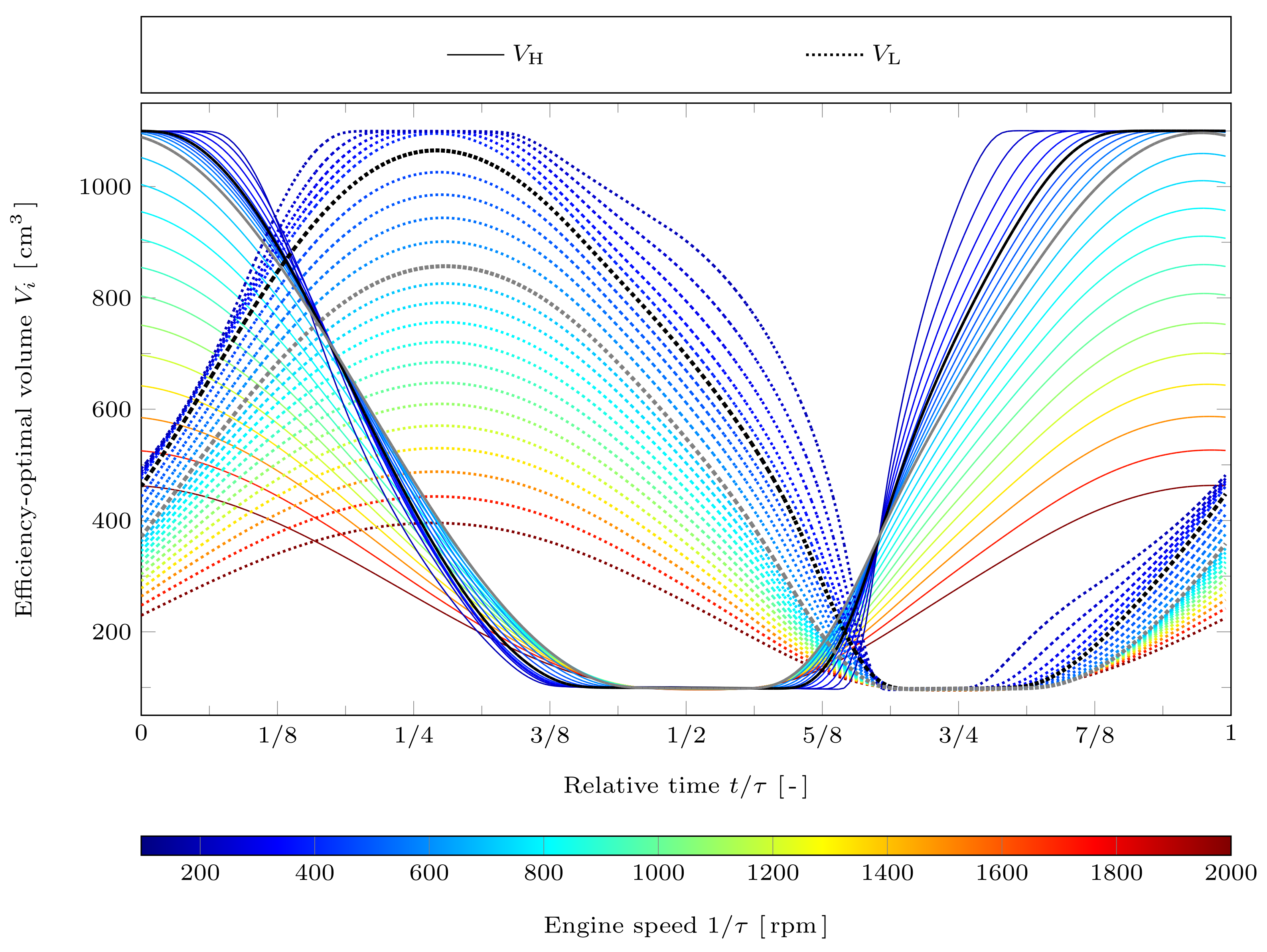
In Figure 3, the Stirling engine’s efficiency-optimal working volume trajectories are shown, again for different engine speeds.

Obviously, the efficiency-optimal volume trajectories are different from the power-optimal ones. The tendency to let the pistons rest in their extreme positions at low engine speeds can also be observed here. However, especially for the cold working volume, this feature is less distinctive than with the power-optimal trajectories. The efficiency-optimal volume trajectories tend to involve smaller piston velocities and reduced swept volumes, when compared to the power-optimal trajectories for the same engine speed. The efficiency-optimal engine speed is ca. 430 rpm, which is highlighted in Figure 3 by thick black lines.

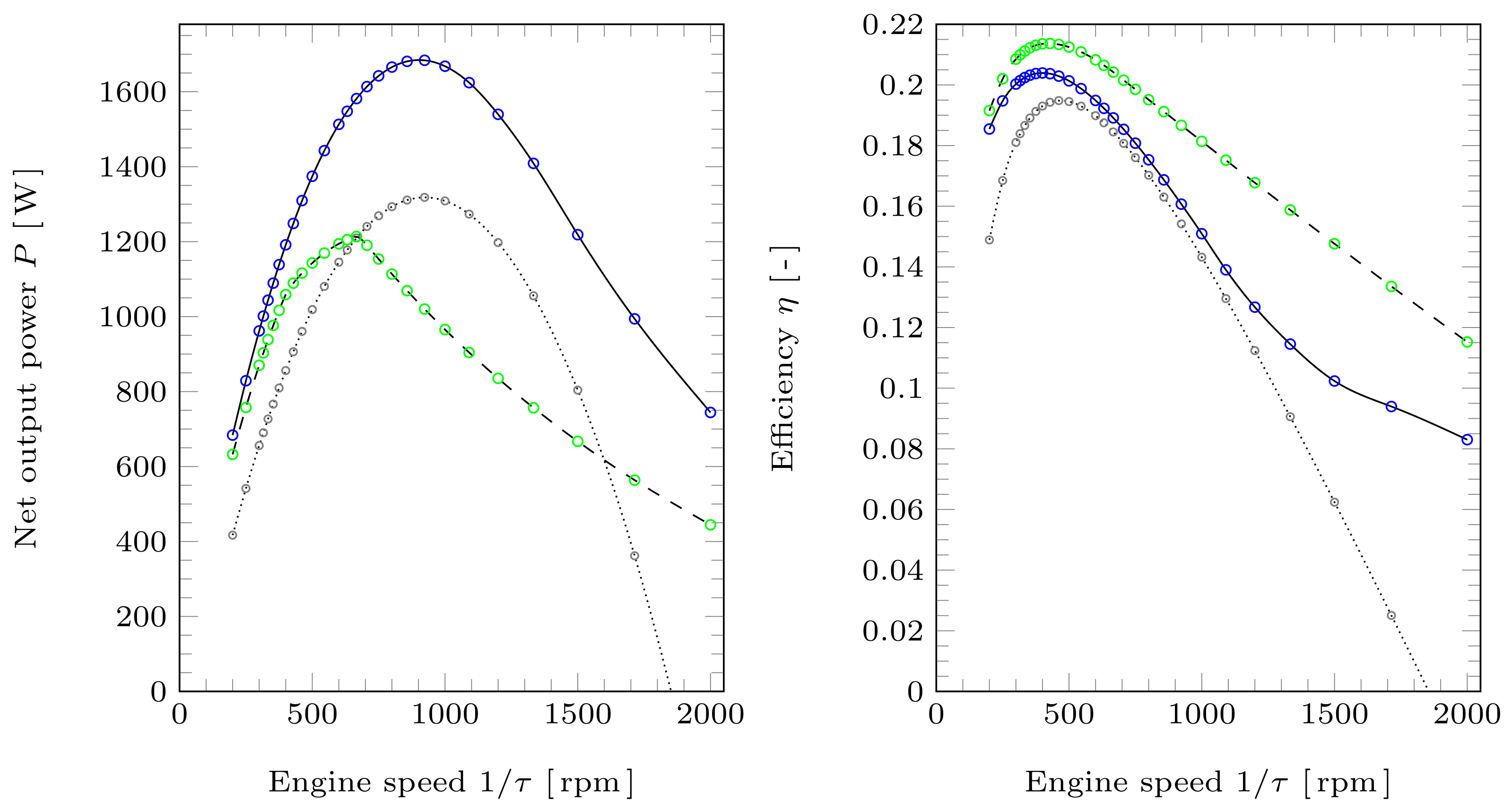
In Figure 4 the Stirling engine’s power and efficiency are plotted against the engine speed for both the power-optimal control (solid, blue) and the efficiency-optimal control (dashed, green). Moreover, the values obtained with the harmonic control (dotted, grey) from which the optimizations were started is shown as a benchmark.

At the maximum power point, the relative power gain due to the power-optimal control is ca. 28%. The relative efficiency gain at the maximum efficiency point, which is achieved with the efficiency-optimal control, is ca. 10%.

Obviously, for a given engine speed, the power-optimal and efficiency-optimal controls each lead to maximum power and maximum efficiency, respectively. However, the optimization for one performance measure may come at the cost of the other. This can, in particular, be seen in the left-hand subfigure for the efficiency-optimal control: For medium engine speeds, the optimization for maximum efficiency leads to remarkable reductions in the output power. There, the power even drops below that obtained with the harmonic control. As opposed to that, the power-optimal control also leads to higher efficiency than the harmonic control over the complete considered range of engine speeds. Note, however, that this may be different for a different set of model parameters.

In the left-hand subfigure of Figure 4, it can be seen that the efficiency-optimal control (green, dashed) leads to a sharp bend at the maximum power point. This occurs at an engine speed of ca. 670 rpm, where the hot working volume trajectory (solid gray line in Figure 3) starts to detach from the maximum volume bound at $t/\tau \approx 1$.

Note that optimal controls obtained with the optimization algorithm introduced above generally constitute local optima. This becomes obvious in Figure 4 when, for example, comparing the powers resulting from the power-optimal controls at $\tau =0.06$ s (1000 rpm) and $\tau =0.12$ s (500 rpm). At $\tau =0.06$ s the power is close to the maximum value, whereas at $\tau =0.12$ s the power is much lower. However, it is clear that the power-optimal control obtained for $\tau =0.06$ s is an admissible periodic control for $\tau =0.12$ s as well, since two oscillations could be performed in one cycle. Hence, the power obtained for $\tau =0.06$ s (1000 rpm) constitutes a lower bound for the global optimum at $\tau =0.12$ s (500 rpm). It can be concluded that the optimal control found for $\tau =0.12$ s (500 rpm) is a local optimum and not the global one. Similar arguments are applicable for the efficiency-optimal control, for example, with the efficiency values obtained at 400 rpm and 200 rpm.

6. Summary

In this paper, we presented an iterative gradient method for optimizing the piston paths of Stirling engines, which is based on Cyclic Optimal Control Theory. After a brief introduction to Stirling engines, we outlined an exemplary irreversible alpha-Stirling engine model. This model served for illustrative purposes and is structured in such a way that its state dynamics can be expressed as a set of coupled ordinary differential equations. The Stirling engine’s state dynamics is influenced by an explicitly time-dependent, vector-valued control function. In particular, this control function determines the temporal paths of the engine’s two working pistons.

The question of which realization of those piston paths—or correspondingly what control function—leads to optimal engine performance regarding a specific objective for a fixed cycle time, constitutes a cyclic optimal control problem. We introduced the necessary conditions of optimality for this problem, involving the definition of a Hamilton function, a path target function, and a set of adjoint ordinary differential equations (costate dynamics). For the optimization of Stirling engines, we presented proper definitions of path target functions to maximize either power or efficiency. Maximum and minimum volume constraints were accounted for here via an additional penalty term in the respective path target function.

Then, we gave a detailed description of an iterative optimization algorithm that starts with a predefined periodic control function, which is gradually shifted over the course of the iterations, so as to gradually enlarge the objective and approach the optimal control. To determine those gradual shifts of the control in every iteration, not only the engine’s state dynamics needs to be solved, but also the costate dynamics. The cyclic optimal control problem features a symmetry that manifests itself in attractive and repulsive limit cycles in the state and costate dynamics, respectively. The algorithm exploits these limit cycles to solve the state and costate dynamics for periodic boundary conditions.

This optimization algorithm was applied to both, power-optimize and efficiency-optimize the control (piston paths) of the above-mentioned exemplary alpha-Stirling engine model for a range of cycle times. The optimization results were compared to piston paths that correspond to a harmonic control with 90${}^{\circ }$ phase shift, which had been used as an initial control for the optimizations. At the maximum power point, the relative power gain due to the power-optimal control is ca. 28%, whereas the relative efficiency gain due to the efficiency-optimal control at the maximum efficiency point is ca. 10%.

The developed optimization algorithm can easily be applied to other Stirling engine models that involve additional irreversibilities or transfer laws that are adapted to describe a specific experimental engine setup. Design limitations such as maximum pressure or maximum piston acceleration can be included in the optimal control problem in terms of additional constraints. Moreover, other types of machines, such as beta-type or free-piston Stirling engines, Stirling cryocoolers, or Vuilleumier refrigerators can be optimized analogously.

7. Conclusions

For the cyclic optimal control problems of a Stirling engine investigated here, we observed that the existence of an attractive limit cycle in the state dynamics translates to a repulsive limit cycle in the costate dynamics. We conclude that a very stable and numerically efficient way to solve such problems is through using indirect iterative gradient algorithms that exploit these limit cycles to solve the state and costate dynamics by temporal forward and backward integration, respectively.

In the case of the considered exemplary Stirling engine, the conducted piston path optimizations lead to significant performance gains of ca. 28% in maximum power and ca. 10% in maximum efficiency. This generally confirms earlier results [22,23,24] and we conclude that it can be very worthwhile to perform such optimizations during the design process of new engines or to improve the control strategy of existing ones. Numerous types of energy conversion systems operate cyclically. We expect that cyclic optimal control theory and, in particular, the developed algorithm can be applied to a wide class of these systems, in order to identify potential performance improvements and enhance their sustainability.

References

- Swedish Stirling AB. Residual Gases—A Huge Market Potential for PWR BLOK. Available online: https://swedishstirling.com/en/marknad/ (accessed on 19 January 2021).
- Microgen Engine Corporation Group. Applications. Available online: https://www.microgen-engine.com/applications/ (accessed on 19 January 2021).
- Azelio. Building a Renewable Future. Available online: https://www.azelio.com/product/ (accessed on 19 January 2021).
- Qnergy. Remote Power. Available online: https://www.qnergy.com/remote-power/ (accessed on 19 January 2021).
- Andresen, B.; Salamon, P.; Berry, R.S. Thermodynamics in Finite Time. Phys. Today 1984, 37, 62–70. [Google Scholar] [CrossRef]
- Andresen, B. Current Trends in Finite-Time Thermodynamics. Angew. Chem. 2011, 50, 2690–2705. [Google Scholar] [CrossRef] [PubMed]
- Rubin, M.H. Optimal Configuration of a Class of Irreversible Heat Engines. I. Phys. Rev. A 1979, 19, 1272–1276. [Google Scholar] [CrossRef]
- Rubin, M.H. Optimal Configuration of a Class of Irreversible Heat Engines. II. Phys. Rev. A 1979, 19, 1277–1289. [Google Scholar] [CrossRef]
- Hoffmann, K.H.; Burzler, J.M.; Schubert, S. Endoreversible Thermodynamics. J. Non Equilib. Thermodyn. 1997, 22, 311–355. [Google Scholar]
- Hoffmann, K.H.; Burzler, J.M.; Fischer, A.; Schaller, M.; Schubert, S. Optimal Process Paths for Endoreversible Systems. J. Non Equilib. Thermodyn. 2003, 28, 233–268. [Google Scholar] [CrossRef]
- Hoffmann, K.H.; Watowich, S.J.; Berry, R.S. Optimal Paths for Thermodynamic Systems: The Ideal Diesel Cycle. J. Appl. Phys. 1985, 58, 2125–2134. [Google Scholar] [CrossRef]
- Burzler, J.M.; Blaudeck, P.; Hoffmann, K.H. Optimal Piston Paths for Diesel Engines. In Thermodynamics of Energy Conversion and Transport; Stanislaw Sieniutycz, S., de Vos, A., Eds.; Springer: New York, NY, USA, 2000; pp. 173–198. [Google Scholar] [CrossRef]
- Chen, L.; Xia, S.; Sun, F. Optimizing piston velocity profile for maximum work output from a generalized radiative law Diesel engine. Math. Comput. Model. 2011, 54, 2051–2063. [Google Scholar] [CrossRef]
- Xia, S.; Chen, L.; Sun, F. Engine performance improved by controlling piston motion: Linear phenomenological law system Diesel cycle. Int. J. Therm. Sci. 2012, 51, 163–174. [Google Scholar] [CrossRef]
- Mozurkewich, M.; Berry, R.S. Optimal Paths for Thermodynamic Systems: The ideal Otto Cycle. J. Appl. Phys. 1982, 53, 34–42. [Google Scholar] [CrossRef]
- Fischer, A.; Hoffmann, K.H. Can a quantitative simulation of an Otto engine be accurately rendered by a simple Novikov model with heat leak? J. Non Equilib. Thermodyn. 2004, 29, 9–28. [Google Scholar] [CrossRef]
- Ge, Y.; Chen, L.; Sun, F. Optimal path of piston motion of irreversible Otto cycle for minimum entropy generation with radiative heat transfer law. J. Energy Inst. 2012, 85, 140–149. [Google Scholar] [CrossRef]
- Watowich, S.J.; Hoffmann, K.H.; Berry, R.S. Intrinsically Irreversible Light-Driven Engine. J. Appl. Phys. 1985, 58, 2893–2901. [Google Scholar] [CrossRef]
- Watowich, S.J.; Hoffmann, K.H.; Berry, R.S. Optimal Paths for a Bimolecular, Light-Driven Engine. Il Nuovo Cim. B 1989, 104, 131–147. [Google Scholar] [CrossRef]
- Ma, K.; Chen, L.; Sun, F. Optimal paths for a light-driven engine with a linear phenomenological heat transfer law. Sci. China Chem. 2010, 53, 917–926. [Google Scholar] [CrossRef]
- Kojima, S. Maximum Work of Free-Piston Stirling Engine Generators. J. Non Equilib. Thermodyn. 2017, 42, 169–186. [Google Scholar] [CrossRef]
- Masser, R.; Khodja, A.; Scheunert, M.; Schwalbe, K.; Fischer, A.; Paul, R.; Hoffmann, K.H. Optimized Piston Motion for an Alpha-Type Stirling Engine. Entropy 2020, 22, 700. [Google Scholar] [CrossRef]
- Scheunert, M.; Masser, R.; Khodja, A.; Paul, R.; Schwalbe, K.; Fischer, A.; Hoffmann, K.H. Power-Optimized Sinusoidal Piston Motion and Its Performance Gain for an Alpha-Type Stirling Engine with Limited Regeneration. Energies 2020, 13, 4564. [Google Scholar] [CrossRef]
- Craun, M.; Bamieh, B. Optimal Periodic Control of an Ideal Stirling Engine Model. J. Dyn. Syst. Meas. Control 2015, 137, 071002. [Google Scholar] [CrossRef] [Green Version]
- Paul, R.R. Optimal Control of Stirling Engines. Ph.D. Thesis, Technische Universität Chemnitz, Chemnitz, Germany, 2020. [Google Scholar]
- Papageorgiou, M.; Leibold, M.; Buss, M. Optimierung—Statische, Dynamische, Stochastische Verfahren für die Anwendung; Springer Vieweg: Berlin/Heidelberg, Germany, 2015. [Google Scholar] [CrossRef]
- Berry, R.S.; Kazakov, V.A.; Sieniutycz, S.; Szwast, Z.; Tsirlin, A.M. Thermodynamic Optimization of Finite-Time Processes; John Wiley & Sons: Chicester, UK, 2000. [Google Scholar]
- Craun, M.J. Modeling and Control of an Actuated Stirling Engine. Ph.D. Thesis, University of California Santa Barbara, Santa Barbara, CA, USA, 2015. [Google Scholar]
- Horn, F.J.M.; Lin, R.C. Periodic processes: A variational approach. Ind. Eng. Chem. Process Des. Dev. 1967, 6, 21–30. [Google Scholar] [CrossRef]
- Kowler, D.E.; Kadlec, R.H. The optimal control of a periodic adsorber: Part II. Theory. AIChE J. 1972, 18, 1212–1219. [Google Scholar] [CrossRef] [Green Version]
- van Noorden, T.L.; Verduyn Lunel, S.M.; Bliek, A. Optimization of cyclically operated reactors and separators. Chem. Eng. Sci. 2003, 58, 4115–4127. [Google Scholar] [CrossRef]
Figure 1.
Schematics of the alpha-type Stirling engine considered. The corresponding endoreversible model [25] has ten degrees of freedom (state variables), being the working space’s volumes , temperatures , and particle numbers , the energies and of the hot and cold halves of the regenerator matrix as well as the particle number and temperature of the gas inside the regenerator dead space.
Figure 2.
Power-optimal trajectories of the working volumes (solid lines) and (dotted lines) of an exemplary alpha-Stirling engine for varying engine speed . The power-optimal engine speed is ca. 920 rpm (thick black lines).
Figure 3.
Efficiency-optimal trajectories of the working volumes (solid lines) and (dotted lines) of an exemplary alpha-Stirling engine for varying engine speed . The efficiency-optimal engine speed is ca. 430 rpm (thick black lines). The power-optimal engine speed for the efficiency-optimal control is ca. 670 rpm (thick gray lines).
Figure 4.
Net output power P and efficiency for the harmonic (gray, dotted), power-optimal (blue, solid), and efficiency-optimal (green, dasehd) control plotted against the engine speed.
Publisher’s Note: MDPI stays neutral with regard to jurisdictional claims in published maps and institutional affiliations. |
© 2021 by the authors. Licensee MDPI, Basel, Switzerland. This article is an open access article distributed under the terms and conditions of the Creative Commons Attribution (CC BY) license (https://creativecommons.org/licenses/by/4.0/).
Share and Cite
MDPI and ACS Style
Paul, R.; Hoffmann, K.H. Cyclic Control Optimization Algorithm for Stirling Engines. Symmetry 2021, 13, 873. https://doi.org/10.3390/sym13050873
AMA Style
Paul R, Hoffmann KH. Cyclic Control Optimization Algorithm for Stirling Engines. Symmetry. 2021; 13(5):873. https://doi.org/10.3390/sym13050873
Chicago/Turabian StylePaul, Raphael, and Karl Heinz Hoffmann. 2021. "Cyclic Control Optimization Algorithm for Stirling Engines" Symmetry 13, no. 5: 873. https://doi.org/10.3390/sym13050873
Note that from the first issue of 2016, this journal uses article numbers instead of page numbers. See further details here.