
Mindlin-Reissner Analytical Model with Curvature for Tunnel Ventilation Shafts Analysis


1
Structures Department, Facultad de Ingeniería Civil, (FIC-UANL), Universidad Autónoma de Nuevo León (UANL), Av. Universidad s/n, Ciudad Universitaria, San Nicolás de los Garza 66455, Mexico
2
Instituto de Ingeniería, Universidad Nacional Autónoma de México (UNAM), Edificio 2, Ciudad Universitaria, C.P. Mexico City 04510, Mexico
*
Author to whom correspondence should be addressed.
Mathematics 2021, 9(10), 1096; https://doi.org/10.3390/math9101096
Submission received: 13 March 2021
/
Revised: 19 April 2021
/
Accepted: 20 April 2021
/
Published: 13 May 2021
(This article belongs to the Special Issue Numerical Analysis and Scientific Computing)
Abstract
:The formulation and analytic solution of a new mathematical model with constitutive curvature for analysis of tunnel ventilation shaft wall is proposed. Based on the Mindlin–Reissner theory for thick shells, this model also takes into account the shell constitutive curvature and considers an expression of the shear correction factor variable in terms of the thickness and the radius of curvature . The main advantage of the proposed model is that it has the possibility to analyze thin, medium and thick tunnel ventilation shafts. As a result, two comparisons were made: the first one, between the new model and the Mindlin–Reissner model without constitutive curvature with the shear correction factor 6 as a constant, and the other, between the new model and the tridimensional numerical models (solids and shells) obtained by finite element method for different slenderness ratios . The limitation of the proposed model is that it is to be formulated for a general linear-elastic and axial-symmetrical state with continuous distribution of the mass.
1. Introduction
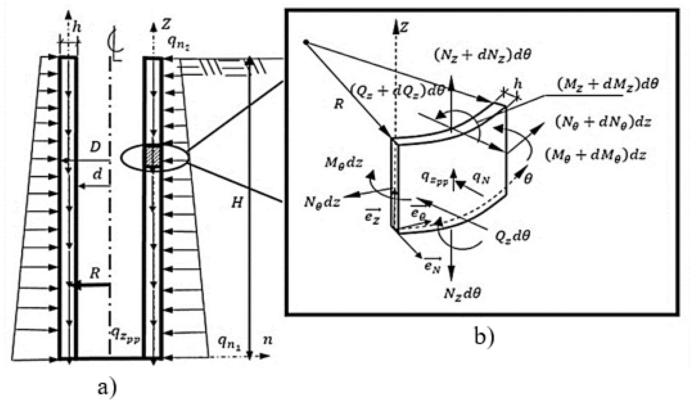
Tunnel ventilation shafts are vertical structural elements for accessing underground structures such as tunnels. The structural analysis of tunnel ventilation shafts is performed through a coaxial cylinder analysis scheme, in axial-symmetrical general state (load, geometry, material and boundary condition) (Figure 1). The importance of designing and building these structures lies in the increasing needs of hydrosanitary network and new means of communications. Thus, an optimum structural design is guaranteed if a reliable analysis method is used.
In the classical shell theory by Goldenveizer and Timoshenko [1,2,3], the three-dimensional continuous solid is modelled by the middle surface of the solid plus the thickness of the shell, Equation (1). This allows the use of the resultant internal forces per unit of arc longitude: bending moment (), shear forces () and membrane axial forces (Figure 1). In addition, Figure 1 also shows the set of variables to be considered.
Resultant internal forces per unit of arc longitude and middle deformations of the shell are related by the integration process inside the thickness of the shell [2,3]. The integration process, defines the constitutive model that will be used in the construction of the mathematical model, in terms of displacement (direct operational model) or in resultant internal forces per unit of arc longitude (inverse operational model).
Equation (2) represents the classical linear-elastic constitutive model that relates the resultant internal forces per unit of arc longitude and the middle deformations of the shell inside the classical shell [1,2,3,4], which presents the following limitations [1,2,5]:
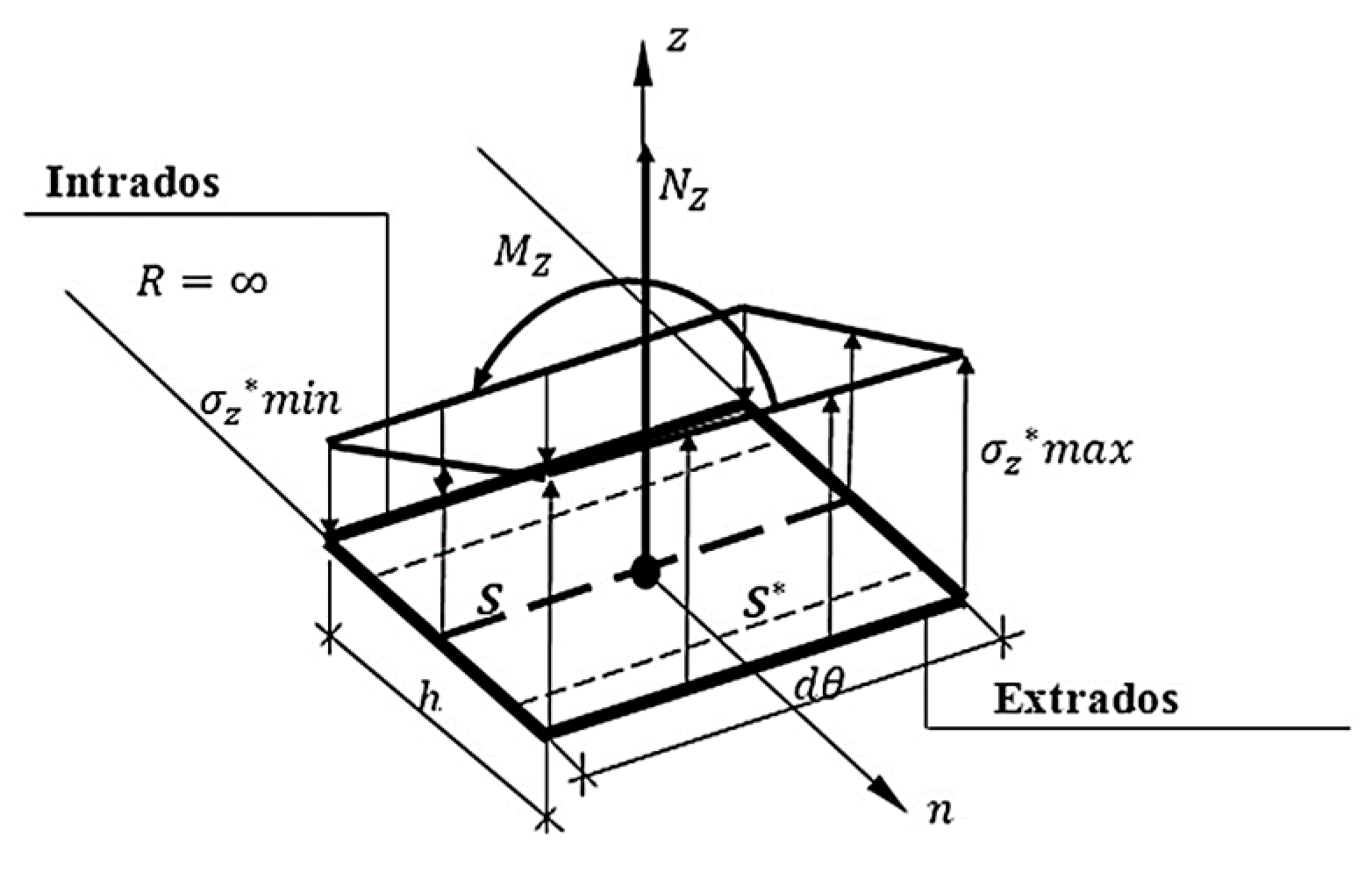
- The model involves a bending of a flat plate plus a membrane behavior without curvature (Figure 2);
- Nonexistence of the constitutive coupling between the membrane forces and the bending moments for any slenderness ratio ;
- Shear correction factor () is employed in the constant shear force, independently of the shell slenderness ratio.
In this paper, a new Mindlin–Reissner mathematical flexural model for tunnel ventilation shafts analysis is obtained; it takes into account the shell constitutive curvature effect [2,3]; along with an update in the shear correction factor () for the shear distribution. A new linear-elastic constitutive relationship between the resultant internal forces per unit of arc longitude and the middle deformations was obtained for the model construction. This constitutive relationship models the constitutive curvature effect in the flexo-compression behavior of the tunnel ventilation shafts. The new model is a generalization of the Love–Kirchhoff and Mindlin–Reissner mathematical models, without constitutive curvature for the analysis scheme of the coaxial cylinder (Figure 1).
2. Coupled Constitutive Model for General Bending of a Coaxial Cylinder
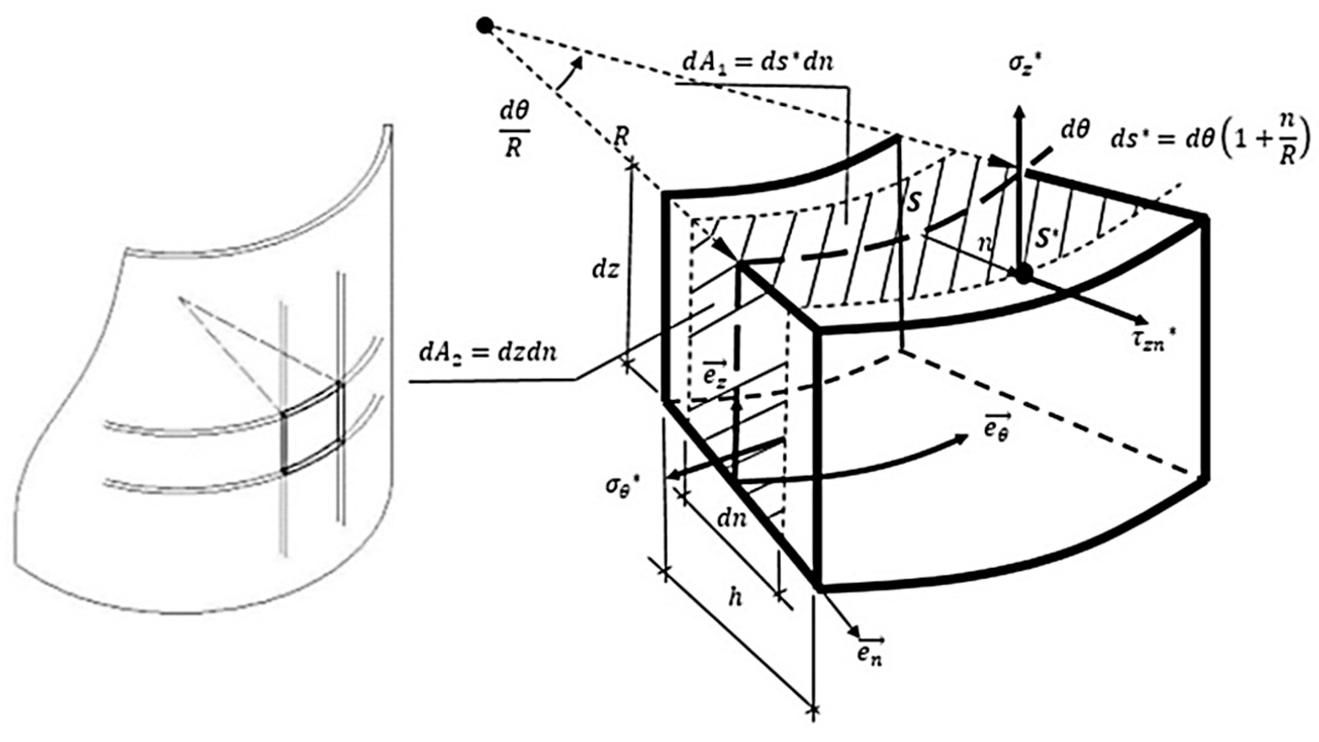
The term represents the differential arc increased in the shell differential arc of the middle surface (Figure 3). Figure 3 shows the stress state in a “differential point” that belong to the surface .
From the stress–strain state definition for the “differential point”, which belong to the surface , Equations (3) and (4), it is possible to integrate the surfaces ( in order to obtain the resultant internal forces per unit of arc longitude: bending moments (), shear and membrane axial forces , Equation (5), Figure 3. The resultant internal forces per unit of arc longitude of the middle surface of the shell in terms of the deformations are obtained by integrating with respect to the axis n. The axis (n) is orthogonal to the middle surface of the shell (Figure 3), Equations (7) and (8). For the integration process, the term , Equation (6), was developed in n potential-function (Taylor series expansion) [3] affecting the integrand with the substitution of the stress-strain state for the “differential point”, Equations (3)–(5).
Equations (7) and (8) show a linear-elastic coupled constitutive model between the membrane forces and the moments for any slenderness ratio of the shell. If the shell curvature is neglected in Equations (7) or (8), the classical shell model, Equation (2), is obtained. In addition, the linear-elastic coupled constitutive model, in Equations (7) and (8), is consistent with the coupled models defined by Galerkin, Novozhilov, Finkel’shtein and Lur’e, and other authors [2,3].
The deformation expressions in terms of the forces and moments, Equation (9), are obtained by inverting the coupled constitutive matrix , Equation (8). It shall be noted that the symmetry on the constitutive matrices, Equations (8) and (9) guarantees the fulfillment of the shell theory general theorems [2,3,6].
Equation (10) represents the coupled constitutive matrix, Equation (8), for an unstiffened orthotropic shell. It is noteworthy that Equation (10) generalizes the constitutive model employed by authors Rotter and Sadowski [4], opening the possibility for future research on this field
The shear correction factor () of constitutive equations, Equations (1), (5), (7)–(9), for parabolic and uniform distributions [7] are obtained from the tangential stress of the energetic equilibrium. If a rectangular and homogeneous section (plate) is considered, the shear correction factor per unit of length is Equation (11) [7], which is the default value of the FEM software [8,9], and corresponds to the classic constitutive model for plates in the Mindlin–Reissner bending state, Equation (1).
By inserting in Equation (11) the shell curvature geometrical relations (Figure 3), an expression for the shear correction factor variable per unit of arc longitude in cross-cylindrical and homogeneous sections is obtained, Equations (12) and (13), which depends on the thickness and the radius of curvature of the shell (Figure 3).
The advantage of the new shear correction factor, Equation (13), is that it takes into account the slenderness ratio of the tunnel ventilation shaft in a geometrical optimization analysis (Table 1).
3. New Mathematical Operational Model
For this study, the internal equilibrium equations generate an equation set of one hyperstatic degree (HD), Equation (14) [1]. The kinematics equations, Equation (15), (Mindlin–Reissner) in cylindrical coordinate associated to Equation (14) can be obtained through the principle of the virtual works (PVW) but also with the transposition method [1,10,11].
By substituting the kinematics equations, Equation (15), and the coupled constitutive equations, Equation (7), into the equilibrium equations, Equation (14), a new mathematical operational model, Equation (16), is obtained, whose unknowns are the middle surface displacement of the shell . Equation (16) generalizes the mathematical model for the isotropic shell presented by Rotter and Sadowski [4].
The analytical solution of the differential set equations, Equation (16), for complex boundary conditions and the inclusion of sections (loads, stiffness, etc.) is inapproachable. However, if the new mathematical model is formulated in terms of the resultant internal forces per unit of arc longitude (inverse operational model), it is possible to obtain an analytical solution of the model.
The compatibility equations of deformations (Saint-Venant identities) and resultant internal forces functions per unit of arc longitude were obtained [12,13] for mathematical modeling in terms of the resultant internal forces per unit of arc longitude.
The new functions for the resultant internal forces per unit of arc longitude, Equation (18), and the new compatibility equation of deformations, Equation (17), were obtained by applying the indeterminate coefficient method (ICM) [14]. By substituting Equation (18) in the internal equilibrium equations of the shell, Equation (14), the equation satisfies itself, which is the general solution of the internal equilibrium of the shell.
By substituting Equation (18) and the coupled constitutive model with curvature, Equation (7), in the compatibility equation of deformations, Equation (17), the new inverse-operational mathematical model is obtained, Equation (19).
The coefficients A1 and B1 from the Equation (19) characterize the influence of the shear and the membrane force facing the bending respectively.
4. Particular Cases
If the constitutive curvature of the shell is disregarded in the mathematical model, Equation (19), the following mathematical model is obtained, Equation (20).
The mathematical model expressed in Equation (20), is a strong-operational formulation in terms of the resultant internal forces per unit of arc longitude of the Mindlin–Reissner flexural model for a coaxial cylinder; and its numerical resolution by FEM (weak-formulation) represents a reference for the analysis of thick shells.
Furthermore, Equation (21) shows a comparative analysis between the second member of the mathematical models, with and without constitutive curvature respectively, Equations (19) and (20). Equation (21) shows the additional effects originated by the axial forces and the orthogonal load model that are not considered in Equation (20).
If the shell constitutive curvature and the shear deformation [15] are disregarded in the general mathematical model, Equation (19), the bending model in operational formulation of Love–Kirchhoff in term of the resultant internal forces per unit of arc longitude is obtained, Equation (22).
Since the dependency between the twist, and the fundamental displacement, are conditioned, the Love–Kirchhoff model for the bending of a coaxial cylinder generates an equality between the hyperstatic degree and the degree of freedom, of the model. This means that the formulation in terms of the resultant internal forces per unit of arc longitude, Equation (22), and the formulation in terms of fundamental displacement, Equation (23), endure to only one differential equation.
5. Analytical Resolution of the New Mathematical Model
The mathematical model, with and without constitutive curvature in terms of the resultant internal forces per unit of arc longitude, Equations (19) and (20), is the nonhomogeneous fourth-order-linear differential equations with constant coefficients. The main difficulty is to obtain its homogeneous solution, due to the shear of each model (terms A and A1). The general solution of the model is the sum of two solutions due to its linearity, Equation (24), i.e., the homogeneous solution, and the particular solution, [21,22].
By applying the general theory of differential equation [21], the homogeneous solution , Equations (27) and (28), is obtained, and the characteristic equation, Equation (25), and the fundamental solution system (F.S.S), Equation (26), are obtained. Out of the two F.S.S, the most employed in engineering is the case due to the fact that the thickness is smaller in comparison with the principal radius of curvature .
If the mathematical condition is evaluated in the new F.S.S, Equation (26), then the general solution of the Love–Kirchhoff model with constitutive isotropy is obtained, Equation (23).
The particular or nonhomogeneous solutions , Equation (30), are obtained by applying the Lagrange’s parameters variation method [21], and depend on the function that operates on the left-hand side term of the differential equations, .
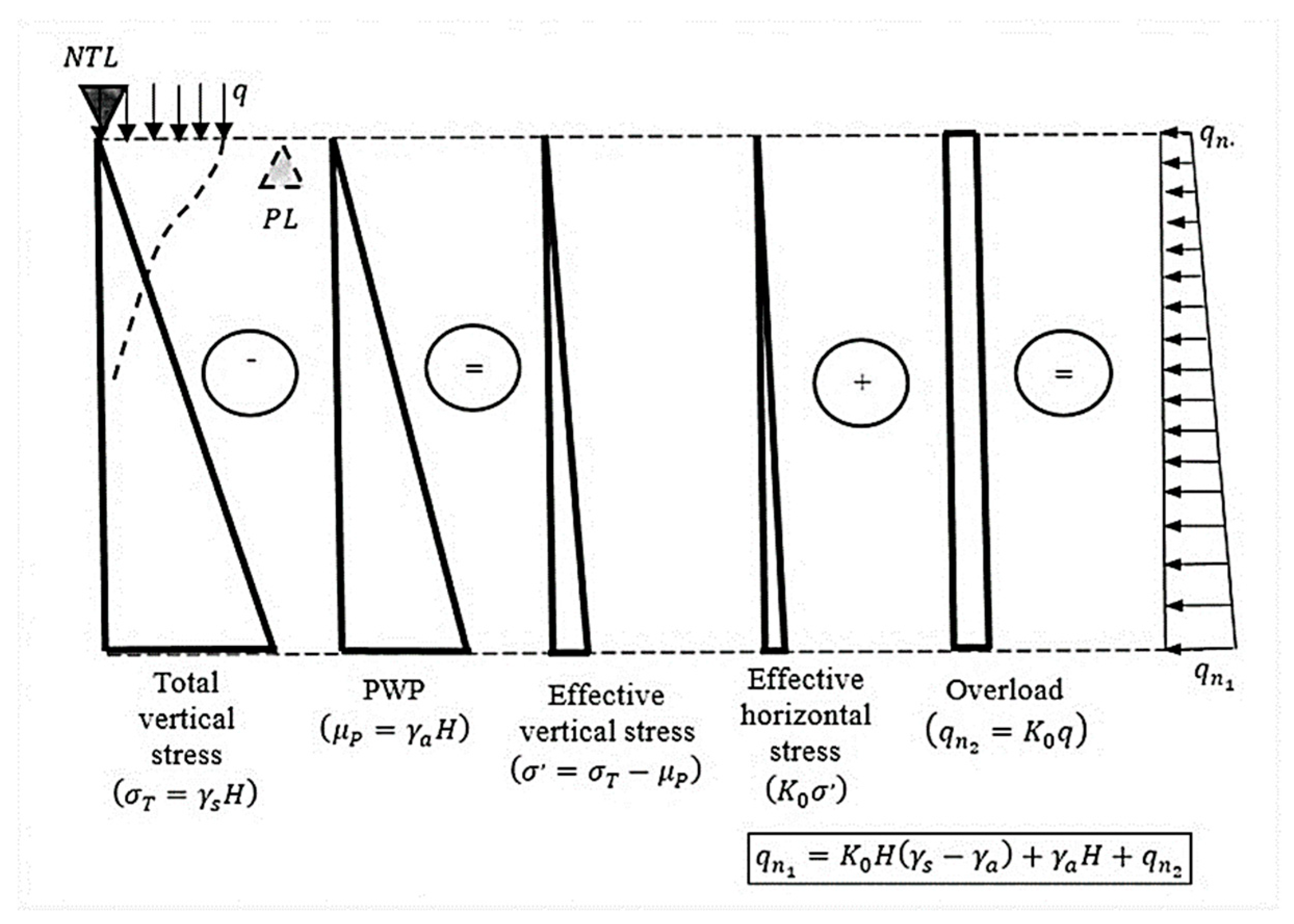
Figure 4 and Equation (29) shows the results when a load model characterized by the own weight of the tunnel ventilation shaft wall, the horizontal effective stress, and the overload action, are defined.’
Once the general solution, Equations (27) and (30), of the resultant internal forces per unit of arc longitude (θ) is obtained, it is necessary to evaluate the boundary conditions imposed on the mathematical model (Table 2) [23]. Six-boundary conditions are required to solve the flexo-compression problem with coupled constitutive curvature (Table 2). Boundary conditions used in EN 1993-1-6 Eurocode [23] were adopted in this paper, along with the Mindlin–Reissner and Timoshenko bending theory particularity.
From a complete and fit definition of the function, the internal forces per unit of arc longitude ) are founded by applying Equation (18). Subsequently, by using the coupled constitutive equations, Equation (10), the deformations on the middle surface of the shell were obtained, and to conclude, the integration process, the displacement field is determined by employing the Mindlin–Reissner kinematics equations, Equation (15). The stress–strain state of the coaxial cylinder is finally obtained through Equations (3) and (4).
6. Numerical Results and Discussions
In this section, fundamental concepts in the shells-analytical and numerical analyses (FEM) in general bending state are illustrated. The physical–mechanical parameters (Table 3) of a typical tunnel ventilation shaft built in the soft soil of Mexico City from Espejel [25] were employed for numerical comparison.
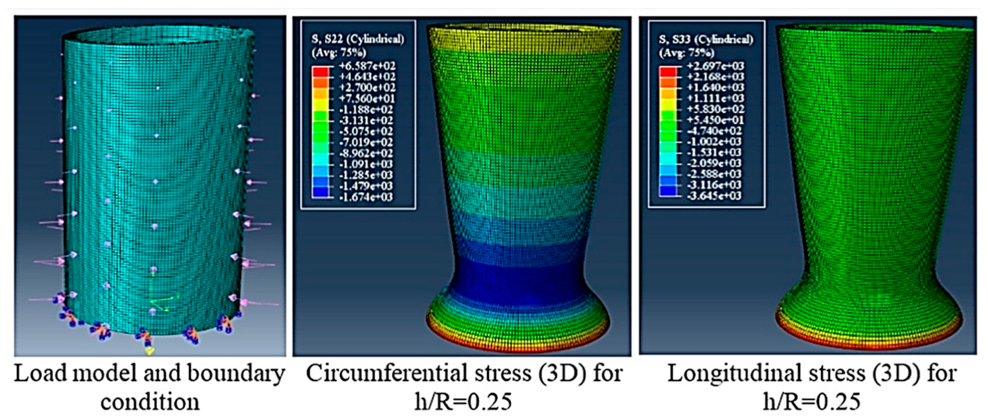
Bearing in mind that there is a continuity between the base and the tunnel ventilation shaft wall, a clamped condition on the cylinder base (BC1r in z = 0) was assumed, along with the free edge on the top (BC1r in z = H). The analytical results (with and without constitutive curvature) were compared with FEM results, using the ABAQUS software [26] (Figure 6 and Figure 7) and considering different formulations (Table 4).
It is known, [7,27,28] that the standard 8-nodes-solid element with complete integration (C3D8), presents a locking-shear problem when used for shells modeling. This problem is bigger when the slenderness increases, and its bending behavior prevails. This numerical locking indicates the incapacity of the interpolation functions (and its gradients) to adapt to solid behavior that often invalidates the obtained solutions [28]. The elements of reduced integration of first and second order (C3D8R and C3D20R), present more precision in flexo-compression problems with bending predominance than the ones corresponding to complete integration-elements, in addition to a reduction in the computing time [26]. The second-order solid elements allow modeling of the curved surfaces with fewer elements, and a greater approximation in areas of high stresses concentration. The shell element S4R is valid for thin or thick-shell problems [26], but it has the disadvantage that it does not obtain the shear per unit of thickness () as output, which allows the subsequent calculation of the transversal stress. The S8R element is valid for thick shell analysis.
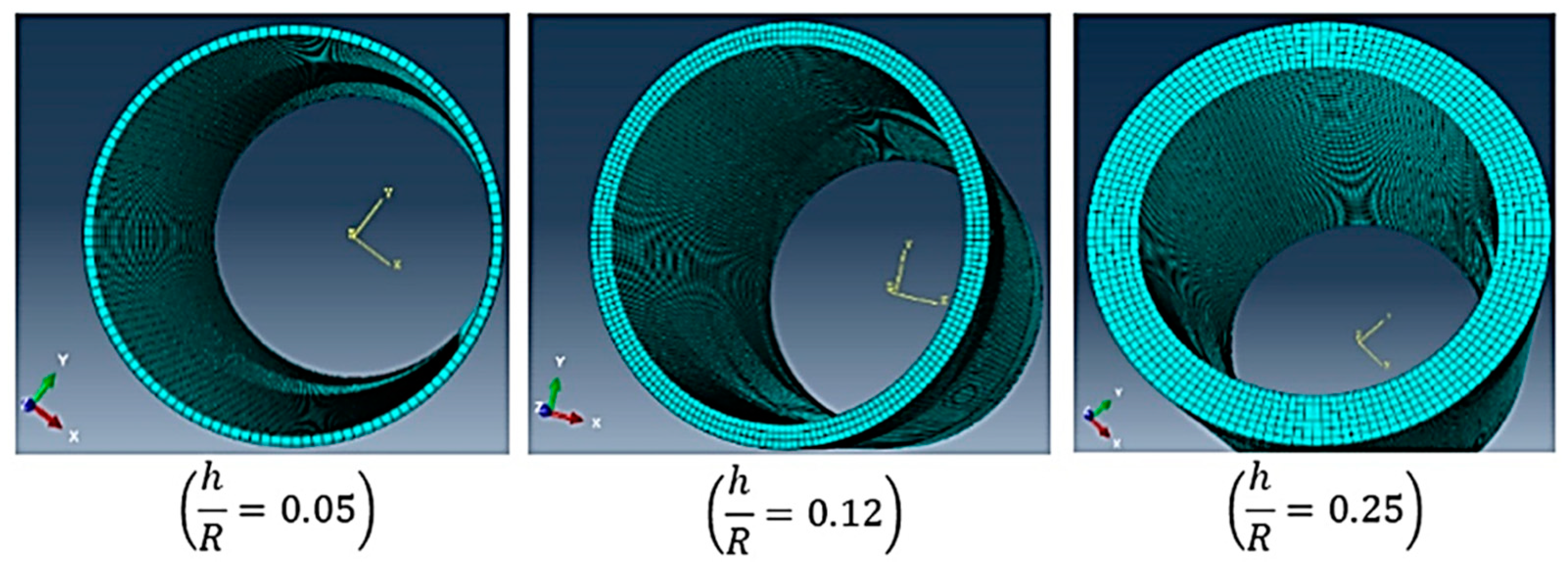
The numerical models used in this paper considered a different slenderness ratio in the shell, and the employment of the shell elements (S4R and S8R) and solid elements (C3D8R and C3D20R) (Table 4 and Figure 6).
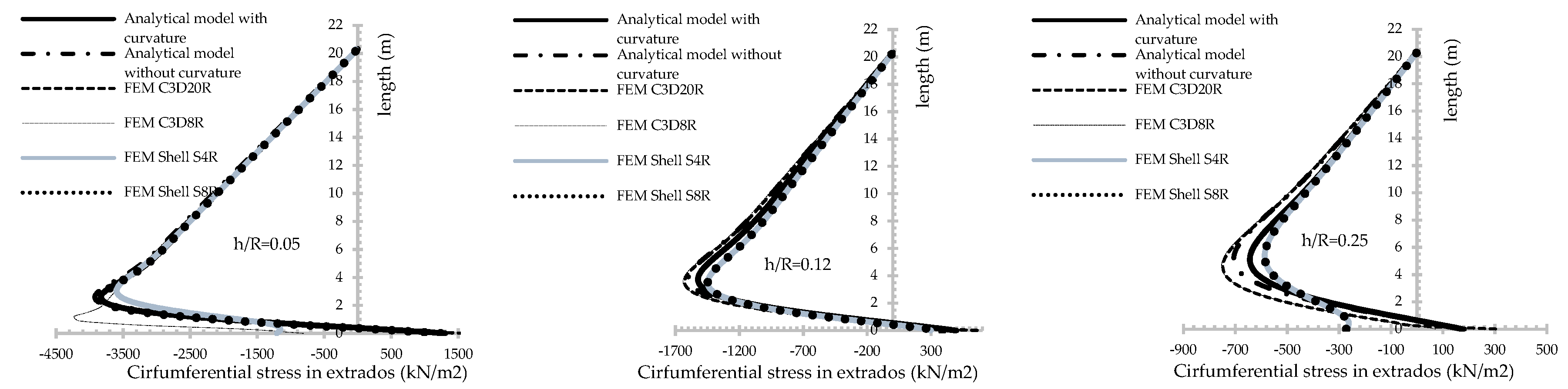
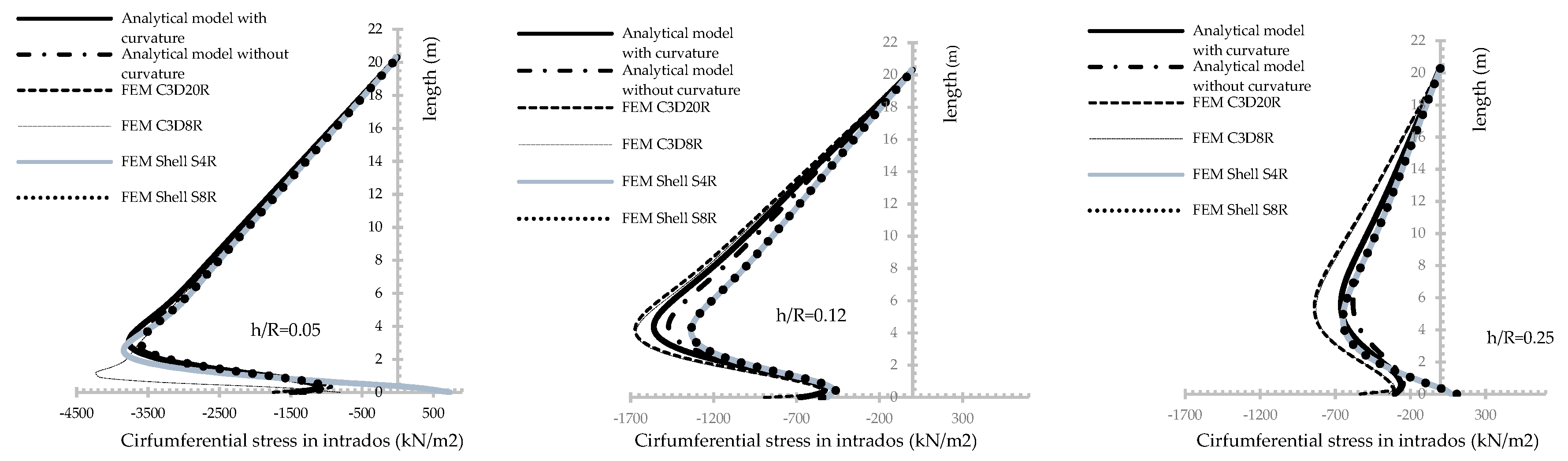
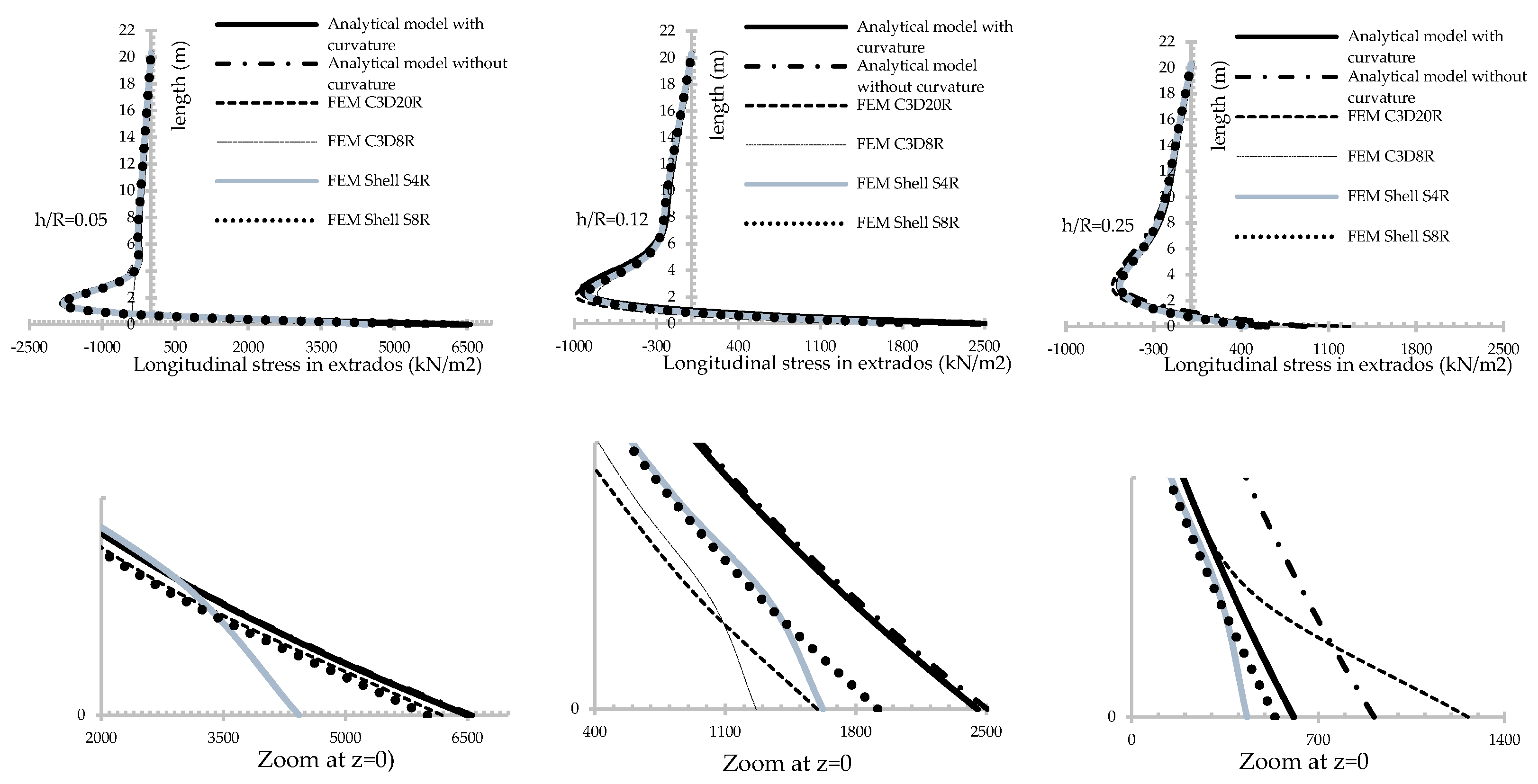
The analytic solution with constitutive curvature shows numerical superiority compared with shell-elements (S8S and S4R) for all results in the entire high of the tunnel ventilation shaft (Figure 8, Figure 9, Figure 10, Figure 11, Figure 12 and Figure 13; Table 5, Table 6, Table 7 and Table 8).
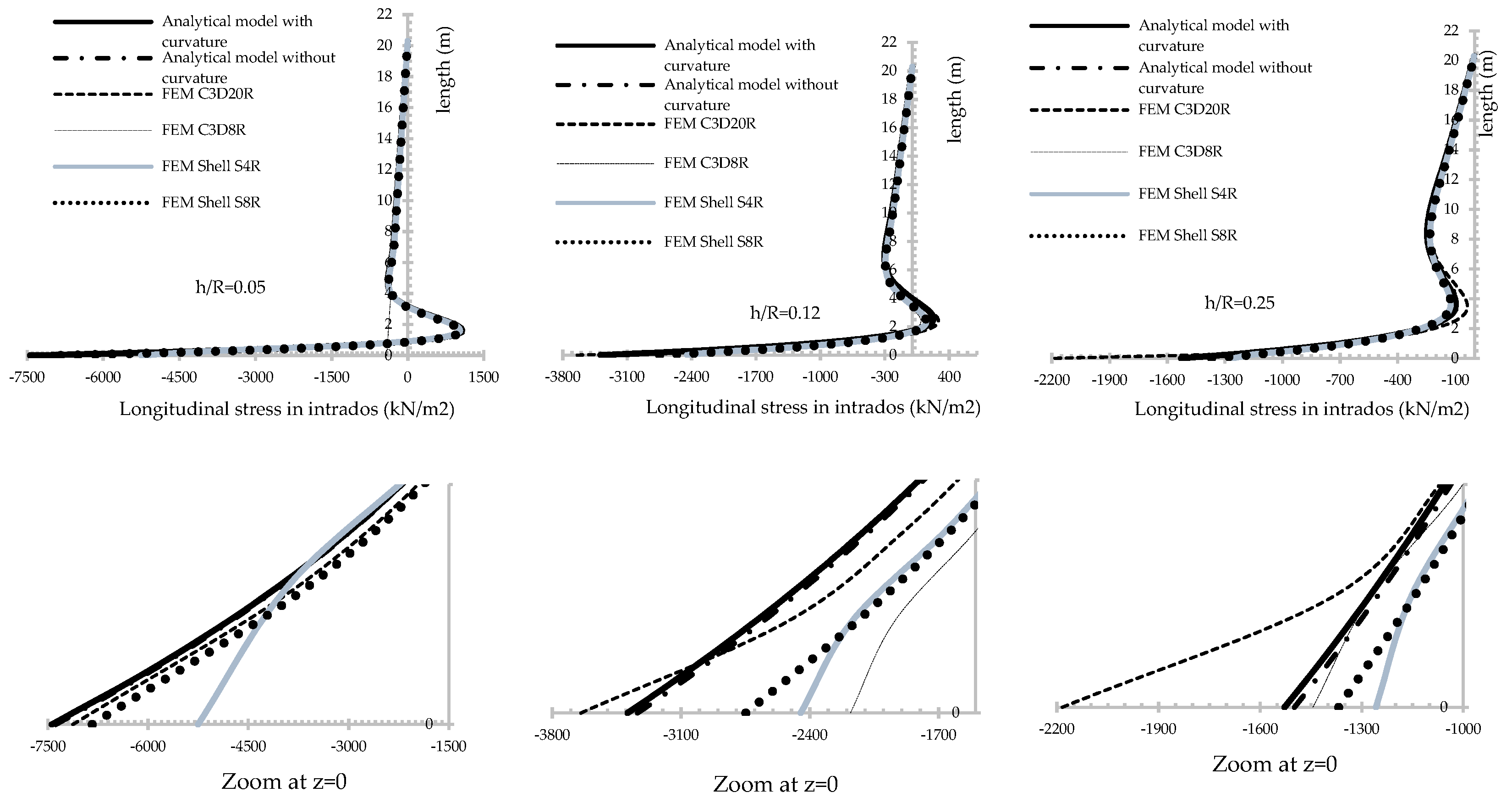
The C3D8R element shows a bad convergence in the obtaining of the maximum longitudinal stress at the base of the cylinder (clamped) (bending concentration) (Table 7 and Table 8). Although, the elements are provide by the Hourglass control [26] there is a stiffness of the shell in that section (Figure 10 and Figure 11). Due to the linearity of the interpolation functions, it is necessary to generate more than one C3D8R element inside the thickness of the shell, which will be able to model the bending concentration in that cross section. The C3D20R element employs trigonometric interpolation functions, which allow modeling with one element into the small thickness of the shell and the stress distribution (circumferential and longitudinal) in the alteration zones [1,3].
For the longitudinal stress (longitudinal flexor-compression), in all shell domains, the analytical solution with constitutive curvature shows numerical superiority than the one obtained through the C3D8R element with more than one element inside the thickness of the shell (Figure 10 and Figure 11; Table 7 and Table 8).
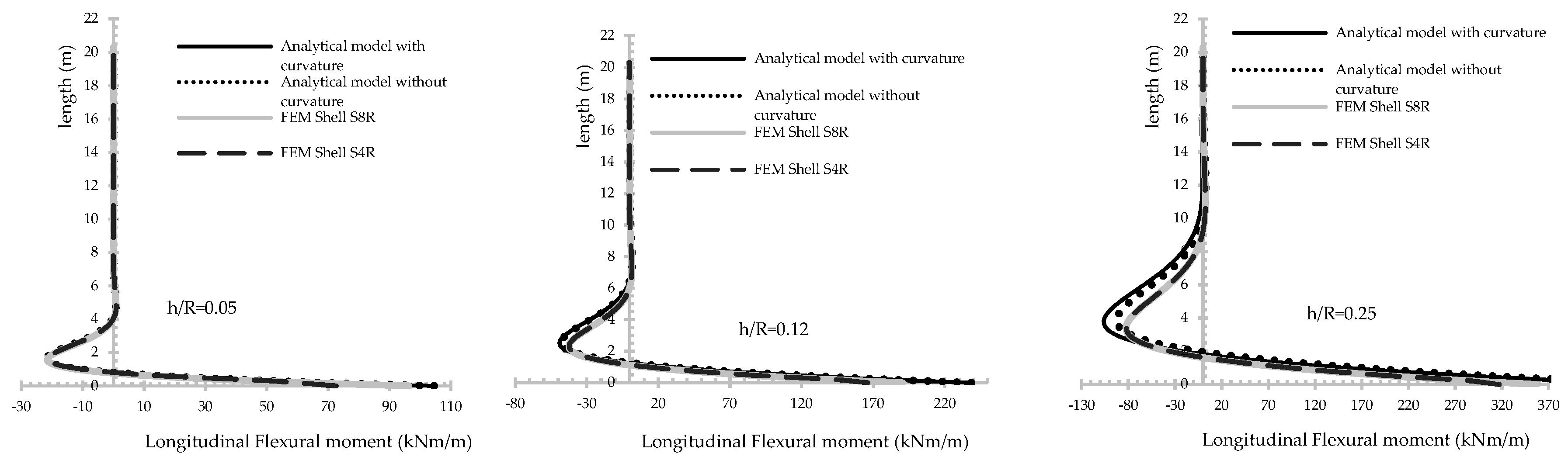
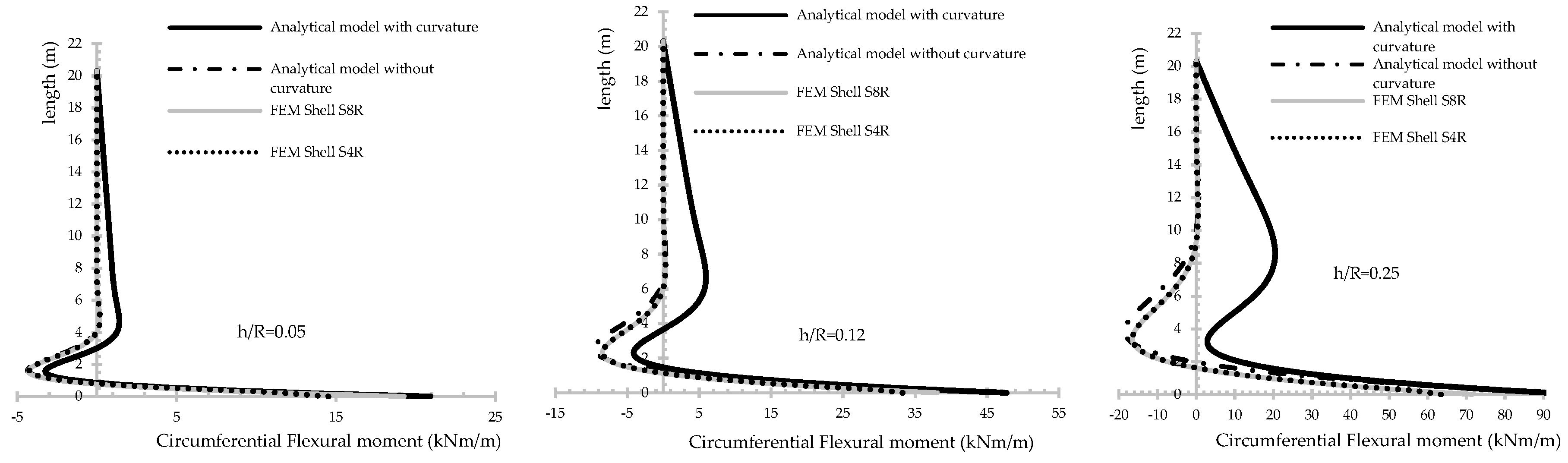
An important aspect for structural design in reinforced concrete is the change in the circumferential flexural moment configuration with the increment of the slenderness ratio of the shell (Figure 13) for analytical solution with constitutive curvature. For a slenderness ratio of 0.25, the studied shell did not have an inversion in the circumferential flexural moment (Figure 13), exalting the physical phenomena that occur: a decreasing of the circumferential negative moment when increasing the slenderness ratio. That is, when the shell is not thin anymore , the bending moment analysis in the circumferential direction is insufficient if the classical constitutive relationship is applied, Equation (31), [1,4,5] on a revolution shell (isotropic, orthotropic and anisotropic) under a general distribution of axial-symmetric pressures.
7. Conclusions
The formulation and analytic solution presented in this paper displays the generality of combining the Mindlin–Reissner theory, the shear correction factor properly for cylindrical shell and the general coupled constitutive model (isotropic and orthotropic) without disregarding the shell curvature from the constitutive.
The proposed mathematical model presents three independent degrees of freedom and it is formulated in terms of the resultant internal forces per unit of arc longitude. This has the advantage of allowing the analysis of cylindrical shell by analytical formulation with thin, medium and thick thickness under a general distribution of axial-symmetric pressures with the very best numerical reliability in the entire shell domain.
Potentially engineering applications include tunnel ventilation shafts, tubular piles under earth pressures, tanks under hydrostatic pressures, reinforced concrete silos under granular solid pressures, gas-filled cisterns, simple alteration effect analysis in thin and medium shells and chimneys. A practical example has been illustrated in a tunnel ventilation shaft analysis for different slenderness ratio , resulting in the following significant conclusions:
- When the isotropic shell is thin, its predominant resistant mechanism is the circumferential membrane force with an inversion of bending moments in the both main directions. From an increase in the slenderness ratio, the flexural contribution in the two main directions dominated the internal equilibrium of the shell and the inserting of the constitutive curvature acquires the biggest importance in the structural response of the shell. For analysis and tunnel ventilation shafts design with slenderness ratio of it is recommendable to insert the constitutive curvature;
- The equations and the general methodology displayed in this paper might be usefully employed in the analysis and design of the cylindrical shell (isotropic and orthotropic) under general distribution of axial-symmetric pressures. The mathematical model formulated in terms of the internal forces per unit of arc longitude allows to solve differential equation systems of multiple degrees of freedom and to model the complex boundary conditions by the Saint-Venant simplification. For this study case, the equations can be applied by means of the basic spreadsheets as tools to assist in the design.
Author Contributions
J.Á.-P.: Conceptualization, Methodology, Formal analysis, Investigation, Writing—Original Draft, Project administration. F.P.: Validation, Data Curation Methodology, Writing—Original Draft, Visualization. All authors have read and agreed to the published version of the manuscript.
Funding
This research received no external funding.
Institutional Review Board Statement
Not applicable.
Informed Consent Statement
Not applicable.
Data Availability Statement
Not report any data.
Acknowledgments
The first author would like to thank the Instituto de Ingeniería UNAM for the postdoctoral grant.
Conflicts of Interest
The authors declare no conflict of interest.
Nomenclature
| Lateral earth pressure plus hydrostatic pressure plus overload on the shaft | |
| External and internal diameter of the shaft, respectively | |
| Body load | |
| Thickness of the wall-shaft (shell thickness) | |
| Principal radius of curvature | |
| Bending moments | |
| Shear force | |
| Membrane-axial forces | |
| Deformations | |
| Displacement | |
| Shaft material weight | |
| Water weight | |
| Soil weight | |
| Coefficient of lateral earth pressure at rest | |
| Shaft height | |
| Cylindrical flexion stiffness of a plate | |
| Membrane stiffness | |
| Elasticity modulus | |
| Poisson ratio | |
| Characteristic longitude of the shell | |
| Discriminant | |
| Shear correction factor | |
| exp | |
| Function with constitutive curvature | |
| Homogeneous function without constitutive curvature | |
| Orthogonal curvilinear coordinates | |
| Solution of the homogeneous equation | |
| Solution of the particular equation. Indeterminate coefficient method | |
| Acronyms used | |
| Fundamental system solution | |
| Hyperstatic Degree | |
| Degree of freedom | |
| Indeterminate coefficient method | |
| Finite element method | |
| Natural terrain level | |
| Phreatic Level | |
| (BC) | Boundary condition |
| Porous water pressure | |
| Note: The term “Constitutive curvature” refers to the inclusion of the shell curvature in the constitutive equations relating the resultant internal forces per unit of arc longitude and the middle shell deformations, Equations (7) and (9). | |
References
- Timoshenko, S.P.; Woinowsky-Krieger, S. Theory of Plates and Shells; McGraw-Hill Book Company: New York, NY, USA, 1959. [Google Scholar]
- Goldenveizer, A.L.; Kaplunov, J.D.; Nolde, E.V. On timoshenko-reissner type theories of plates and shells. Int. J. Solids Struct. 1993, 30, 675–694. [Google Scholar] [CrossRef]
- Goldenveizer, A.L. Theory of Elastic Thin Shells; Pergamon Press for A.S.M.E.: Pergamon, Turkey, 1976. (In Russian) [Google Scholar]
- Rotter, J.M.; Sadowski, A.J. Cylindrical shell bendind theory for orthotropic shells under general axisymmetric pressure distributions. Eng. Struct. 2012, 42, 258–265. [Google Scholar] [CrossRef] [Green Version]
- Nerubalio, A.B.; Nerubalio, F. Generalization of Vlasov’s equations for a cylindrical shell to the case of a transversely isotropic material. J. Appl. Mech. Techincal Phys. 2005, 46, 564–569. [Google Scholar] [CrossRef]
- Goldenveizer, A.L. On algorithms of asymptotic derivation of two-dimensional shell theory and Saint-Venant principle. J. Appl. Math. Mech. 1994, 58, 96–108. [Google Scholar]
- Oñate, E. Structural Analysis with the Finite Element Method. Linear Statics: Volume 1: Basis and Solids; Springer: Berlin/Heidelberg, Germany, 2009. [Google Scholar]
- DIANA. User’s Manual—Element Library; TNO DIANA BV: Delft, The Netherlands, 2017. [Google Scholar]
- MIDAS. Engineering Software, 2016. MIDAS FEA: Analysis and algorithm. Midas Engineering Software. Available online: https://www.midasoft.com/ebook/structural-analysis-guide (accessed on 2 April 2021).
- Castañeda, A.E.; Cobelo, W.; González, Y.; Álvarez, J. A look at half a century of shells foundations, methods of calculation and associate research in Cuba. J. Constr. Cathol. Univ. Chile 2011, 26, 245–268. (In Spanish) [Google Scholar]
- Hernández(Pimpo), J.E. Unified Approach to the Membrane Theory of Shells; Centro de Informacion Cientifica y Tecnica, Universidad de la Habana: La Habana, Cuba, 1972; pp. 21–34. [Google Scholar]
- Timoshenko, S.P.; Goodier, N. Elasticity Theory; McGraw-Hill Book Company: New York, NY, USA, 1970. [Google Scholar]
- Ignaczak, J.; Hetnarski, R. Mathematic Theory of Elasticity; McGraw-Hill Book Company: New York, NY, USA, 1956. [Google Scholar]
- Álvarez, J. Inverse Formulation of Shell in Relative Coordinate with Projected Deformations. Ph.D. Thesis, Technological University of Havana, La Habana, Cuba, 2014. (In Spanish). [Google Scholar]
- Novozhilov, V.V. The Theory of Thin Shells; Sudpromgiz: Leningrad, Russia, 1962. (In Russian) [Google Scholar]
- Hamdan, M.N.; Abuzed, O.; Al-Salaymeh, A. Assessment of an edge type settlement of above ground liquid storage tanks using a simple beam model. Appl. Math. Model. 2007, 31, 2461–2474. [Google Scholar] [CrossRef]
- Caneiro, J.A.H.; Hernández, J.P. Analysis of superficial cylindrical circumferencially prestressed tanks. Rev. Obras Públicas 1999, 29–38. (In Spanish) [Google Scholar]
- Kukreti, A.R.; Zaman, M.M.; Issa, A. Analysis of fluid storage tanks including foundation-superstructure interaction. Appl. Math. Model. 1993, 17, 618–631. [Google Scholar] [CrossRef]
- Quanwei, R.; Hongjiong, T. Numerical solution of the static beam problem by Bernoulli collocation method. Appl. Math. Model. 2016, 40, 193–205. [Google Scholar]
- Vilardell, J.M. Structural Analysis and Cylindrical Deposit Criteria for Pre-Stressed Concretes; Channels and Ports: Barcelona, Spain, 1994. (In Spanish) [Google Scholar]
- Aulduchateau, P.; Zachmann, D. Theory and Problems of Partial Differential Equations; McGraw-Hill Book Company: New York, NY, USA, 2010. [Google Scholar]
- Bronson, R.; Costa, G. Differential Equations; McGraw-Hill Companies: New York, NY, USA, 2009. [Google Scholar] [CrossRef]
- Eurocode, E.N. 1991-6. Eurocode 3: Design of Steel Structures, Part1–6: Strengh and Stability of Shell Structures; Eurocode, Ed.; Comité Européen de Normalisation: Brussels, Belgium, 2007. [Google Scholar]
- R2014b, MV. Mathlab (Matrix Laboratory and Guide); Mathlab V R2014b App Building; MathWorks: Natick, MA, USA, 2014.
- Espejel, O.A.; Castro, C.J.; Mena, E. Structural design of Shaft and Tunnel. In Studies; Calculation Memory of Executive Project; The Instituto de Ingeniería UNAM: Chalco, Mexico, 2003. (In Spanish) [Google Scholar]
- Abaqus. Analysis user´s manual. In Documentation; Dassault Systemes Simulia Corporation: Mason, OH, USA, 2016. [Google Scholar]
- Eduardo, N.D. A continuum mechanics based four-node shell element for general non-linear analysis. Eng. Comput. 1984, 1, 77–88. [Google Scholar]
- Flores, F.G.; Oñate, E. A solid finite element with an improvement in the transverse shear behavior for shell analysis. Métodos Numéricos Para Cálculo Diseño Ing. 2011, 27, 258–268. (In Spanish) [Google Scholar] [CrossRef] [Green Version]
Figure 1.
Mechanical model of tunnel ventilation shafts building by “floating shafts” construction system, (a) Analysis scheme for shafts, (b) Free body diagram of shaft differential slice
Figure 1.
Mechanical model of tunnel ventilation shafts building by “floating shafts” construction system, (a) Analysis scheme for shafts, (b) Free body diagram of shaft differential slice

Figure 2.
Linear distribution of the normal stress disregarding the constitutive curvature of the shell.
Figure 2.
Linear distribution of the normal stress disregarding the constitutive curvature of the shell.

Figure 3.
Geometrical details for modeling the shell curvature in the free body diagram of the tunnel ventilation shaft differential slide.
Figure 3.
Geometrical details for modeling the shell curvature in the free body diagram of the tunnel ventilation shaft differential slide.

Figure 4.
Load model.

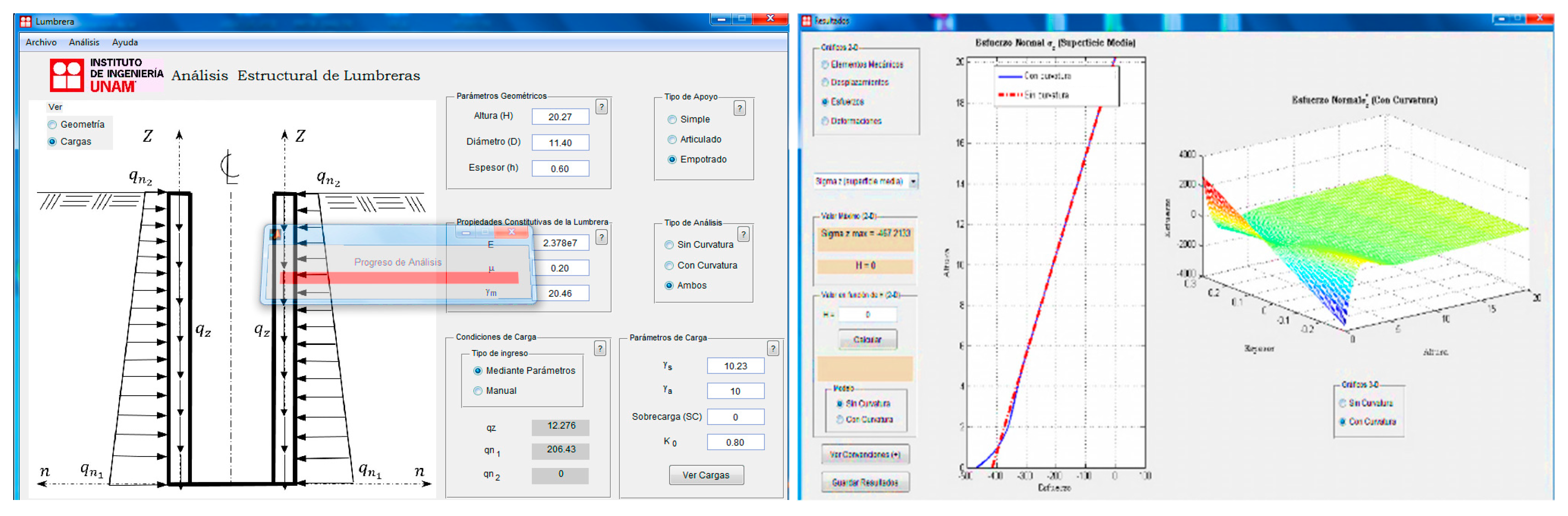
Figure 5.
Program analysis and viewer results.

Figure 6.
Meshing for different slenderness ratio with finite element solid 3D.

Figure 7.
Details of the numerical model in Abaqus.

Figure 8.
Circumferential stress in extrados for thin, medium and thick shells, considering different models.
Figure 8.
Circumferential stress in extrados for thin, medium and thick shells, considering different models.

Figure 9.
Circumferential stress in intrados for thin, medium and thick shells, considering different models.
Figure 9.
Circumferential stress in intrados for thin, medium and thick shells, considering different models.

Figure 10.
Longitudinal stress in intrados for thin, medium and thick shells, considering different models.
Figure 10.
Longitudinal stress in intrados for thin, medium and thick shells, considering different models.

Figure 11.
Longitudinal stress in extrados for thin, medium and thick shells, considering different models.
Figure 11.
Longitudinal stress in extrados for thin, medium and thick shells, considering different models.

Figure 12.
Longitudinal flexural moment for thin, medium and thick shells, considering different models.
Figure 12.
Longitudinal flexural moment for thin, medium and thick shells, considering different models.

Figure 13.
Circumferential flexural moment for thin, medium and thick shells, considering different models.
Figure 13.
Circumferential flexural moment for thin, medium and thick shells, considering different models.


Table 1.
Comparison between the new shear correction factor for tunnel ventilation shafts, and the shear correction factor for plates for different slenderness ratios .
Table 1.
Comparison between the new shear correction factor for tunnel ventilation shafts, and the shear correction factor for plates for different slenderness ratios .
| Relative Error (%) | |||
|---|---|---|---|
Shafts was assumed as a pattern.
Table 2.
Comparison between the new shear correction factor for tunnel ventilation shafts, and the shear correction factor for plates for different slenderness ratio .
Table 2.
Comparison between the new shear correction factor for tunnel ventilation shafts, and the shear correction factor for plates for different slenderness ratio .
| ID | Simple Term | ||
|---|---|---|---|
| BC1 r | Clamped | and | |
| BC1 f | and | ||
| BC2 r | Pinned | and | |
| BC2 f | and | ||
| BC3 | Free edge | and |
Table 3.
Physical, mechanical and geometrical properties of the tunnel ventilation shaft N°1 of the project-“Río La Compañia” from Espejel.
Table 3.
Physical, mechanical and geometrical properties of the tunnel ventilation shaft N°1 of the project-“Río La Compañia” from Espejel.
| Physical and Mechanical Properties |
| Geometrical Properties |
Table 4.
Finite element types and statistical meshing.
| Finite Element Type Description | |||||||
|---|---|---|---|---|---|---|---|
| Nodes | Elements | Nodes | Elements | Nodes | Elements | ||
| Solid elements 3D | C3D20R: A 20-node quadratic brick, reduced integration | 59,644 | 8432 | 289,708 | 57,528 | 326,636 | 71,928 |
| C3D8R: An 8-node linear brick, reduced integration, hourglass control | 17,112 | 8432 | 77,456 | 57,528 | 84,952 | 71,928 | |
| Shell elements | S8R: An 8-node doubly curved thick shell, reduced integration | 8694 | 8568 | 8694 | 8568 | 8694 | 8568 |
| S4R: A 4-node doubly curved thin or thick shell, reduced integration, hourglass control, finite membrane strains | 25,956 | 8568 | 25,956 | 8568 | 25,956 | 8568 | |
Table 5.
Maximum circumferential stress in extrados for different slenderness ratio.
| Length (m) | ||||||||||||
|---|---|---|---|---|---|---|---|---|---|---|---|---|
| Analytical Solution | FEM Shells | FEM 3D | ||||||||||
| With CC | Without CC | % EA | S4R | % ES4R | S8R | % ES8R | C3D8R | % EC3D8R | C3D20R | % EA-C3D20R | ||
| 0.05 | 2.57 | 3833.002 | 3923.135 | 2.35 | 3596.92 | 6.16 | 3773.11 | 1.59 | 3730.3 | 0.514 | 3749.56 | 2.225 |
| 0.12 | 3.73 | 1523.094 | 1601.1821 | 5.13 | 1447.13 | 4.99 | 1447.63 | 5.21 | 1640.83 | 0.787 | 1628.02 | 6.445 |
| 0.25 | 5.1 | 644.19 | 706.634 | 9.69 | 586.868 | 8.90 | 587.301 | 9.69 | 752.557 | 0.557 | 748.391 | 13.923 |
| Where: | CC: Constitutive curvature; EA: relative error between the analytical results (pattern: analytical solution with CC); ES4R: relative error between the analytical result with CC and shell element S4R (pattern: analytical solution with CC); ES8R: relative error between the analytical result with CC and shell element S8R (pattern: analytical solution with CC); EC3D8R: relative error between the elements C3D8R and C3D20R (pattern: C3D20R); EA-C3D20R: relative error between the analytical result with CC and the element C3D20R (pattern: C3D20R). | |||||||||||
Table 6.
Maximum circumferential stress in intrados for different slenderness.
| Length (m) | ||||||||||||
|---|---|---|---|---|---|---|---|---|---|---|---|---|
| Analytical Solution | FEM Shells | FEM 3D | ||||||||||
| With CC | Without CC | % EA | S4R | % ES4R | S8R | % ES8R | C3D8R | % EC3D8R | C3D20R | % EA-C3D20R | ||
| 0.05 | 3.06 | 3770.237 | 3673.337 | 2.57 | 3834.26 | 1.70 | 3599.85 | 4.52 | 3619.5 | 4.517 | 3790.72 | 0.543 |
| 0.12 | 4.38 | 1560.739 | 1471.875 | 5.69 | 1335.59 | 14.43 | 1336.09 | 14.39 | 1665.84 | 0.471 | 1673.72 | 7.239 |
| 0.25 | 5.85 | 712.314 | 634.328 | 10.95 | 649.409 | 8.83 | 649.813 | 8.77 | 828.22 | 1.459 | 840.48 | 17.993 |
| See Table 5 for legend | ||||||||||||
Table 7.
Maximum longitudinal stress in extrados for different slenderness ratio.
| Analytical Solution | FEM Shells | FEM 3D | |||||||||
|---|---|---|---|---|---|---|---|---|---|---|---|
| With CC | Without CC | % EA | S4R | % ES4R | S8R | % ES8R | C3D8R | % EC3D8R | C3D20R | % EA-C3D20R | |
| 0.05 | 6500.02 | 6556.31 | 0.87 | 4429.12 | 31.860 | 6006.91 | 7.586 | 412.305 | 93.334 | 6184.77 | 5.097 |
| 0.12 | 2452.9 | 2506.165 | 2.17 | 1623.46 | 33.815 | 1917.51 | 21.827 | 1265.24 | 53.086 | 2696.94 | 9.049 |
| 0.25 | 861.4145 | 910.11 | 5.65 | 432.582 | 49.782 | 537.565 | 37.595 | 535.274 | 57.637 | 1263.55 | 31.826 |
| See Table 5 for legend | |||||||||||
Table 8.
Maximum longitudinal stress in intrados for different slenderness ratio.
| Analytical Solution | FEM Shells | FEM 3D | |||||||||
|---|---|---|---|---|---|---|---|---|---|---|---|
| With CC | Without CC | % EA | S4R | % ES4R | S8R | % ES8R | C3D8R | % EC3D8R | C3D20R | % EA-C3D20R | |
| 0.05 | 7444.063 | 7386.986 | 0.77 | 5253.69 | 29.424 | 6837.6 | 8.147 | 412.305 | 94.214 | 7126.37 | 4.458 |
| 0.12 | 3390.943 | 3336.8407 | 1.60 | 2450.06 | 27.747 | 2748.18 | 18.955 | 2179.69 | 40.199 | 3644.93 | 6.968 |
| 0.25 | 1790.302 | 1740.786 | 2.77 | 1258.13 | 29.725 | 1368.24 | 23.575 | 1444.26 | 33.889 | 2184.61 | 18.049 |
| See Table 5 for legend | |||||||||||
Publisher’s Note: MDPI stays neutral with regard to jurisdictional claims in published maps and institutional affiliations. |
© 2021 by the authors. Licensee MDPI, Basel, Switzerland. This article is an open access article distributed under the terms and conditions of the Creative Commons Attribution (CC BY) license (https://creativecommons.org/licenses/by/4.0/).
Share and Cite
MDPI and ACS Style
Álvarez-Pérez, J.; Peña, F. Mindlin-Reissner Analytical Model with Curvature for Tunnel Ventilation Shafts Analysis. Mathematics 2021, 9, 1096. https://doi.org/10.3390/math9101096
AMA Style
Álvarez-Pérez J, Peña F. Mindlin-Reissner Analytical Model with Curvature for Tunnel Ventilation Shafts Analysis. Mathematics. 2021; 9(10):1096. https://doi.org/10.3390/math9101096
Chicago/Turabian StyleÁlvarez-Pérez, José, and Fernando Peña. 2021. "Mindlin-Reissner Analytical Model with Curvature for Tunnel Ventilation Shafts Analysis" Mathematics 9, no. 10: 1096. https://doi.org/10.3390/math9101096
Note that from the first issue of 2016, this journal uses article numbers instead of page numbers. See further details here.