Information Use and the Condorcet Jury Theorem

Abstract

Using a simple model of a coordination game, this paper explores how the information use of individuals affects an optimal committee size. Although enlarging the committee promotes information aggregation, it also stimulates the members’ coordination motive and distorts their voting behavior through higher-order beliefs. On the determination of a finite optimal committee size, the direction and degree of strategic interactions matter. When the strategic complementarity among members is strong, a finite optimal committee size exists. In contrast, it does not exist under strategic substitution. This mechanism is applied to the design of monetary policy committees in a New Keynesian model in which a committee conducts monetary policy under imperfect information.

1. Introduction

The economic theory of committee decision-making has developed rapidly in recent years. The background of this stream is not only the progress of economic theory but also that decision-making by committees plays an important role in economic activities. Many countries traditionally adopt jury systems, and their design problems have been one of the central subjects of the academic and practical arguments in committee design. As the latest event, Japan brought the citizen judge system into effect in 2009 and its design problem was and will be discussed effectively. Another outstanding example is the recent establishment of monetary policy committees in many countries. For example, Bank of England and Bank of Japan founded the Monetary Policy Committee in 1997 and the Policy Board in 1998, respectively, and the central banks of the other countries followed them consecutively. Besides, the governments of many countries traditionally call well-informed persons to the committees for important policy issues, such as tax reforms. Big firms hold meetings to make decisions on important matters for their business. Following this trend, the demand for committee design is growing day by day.

The problem of forming optimal committee sizes is an important issue in committee decision-making. The most fundamental argument is whether or not we can increase the performance of the committees (unlimitedly) by increasing the number of the committee members (infinitely). A famous answer for it is Condorcet’s [1] jury theorem. The theorem asserts that when the committee members vote honestly by use of their own information, enlarging the committee always raises the probability that the committee makes an appropriate decision, and it converges to one as the committee size goes to infinity. This implies that finite optimal sizes of committees do not exist. The result is intuitive in a sense but there are several critical arguments against it in recent literature. They dispute Condorcet’s assertion, mainly focusing on the belief that information acquisition of the committee members is costly in the real world and this affects the members’ behavior as follows. When the committee size is large, the committee members avoid paying the information acquisition cost and free-ride on the information that the other members provide. This is because their contribution to the decision of the committee is small, given the information acquisition cost. Thus, the Condorcet jury theorem can fail to hold under the existence of the information acquisition cost: See Li [2] for the free-rider problem and Gerling et al. [3] for a survey.

In this paper, I use an approach different from that of existing studies to discuss the optimal committee size. I focus on the role of coordination behavior among committee members with information. In the case of jury systems, although individual names of jurors are not disclosed, trials by courts are held publicly and their sayings are documented and reported. When individual jurors face uncertainty, they may avoid distant voting from the general tendency in the jury. Besides, many organizations have instituted the rules of information disclosure in recent years. In particular, disclosure of public information on the policy issues of the government and central bank has usually been a legal mandate in many developed countries.

How does such an institutional trend make a difference in committee decision-making? Such transparency can generate the incentive of the committee members to coordinate with the other members because the minutes are often opened to the public. Hence the individual member faces an accountability problem. Using a simple game-theoretic model, Prat [4] argues that with carrier concern, transparency generates herding and conformism among committee members, distorting their voting: See also Visser and Swank [5]. Fehrler and Hughes [6] confirm that transparency foments conformism through an experiment. In contrast, some studies show that transparency can lead to anti-herding and exaggeration: Levy [7,8]. Thus, to consider the general class of coordination, the model of the present paper considers the two cases where the committee members have an incentive to keep their votes on and away from the others’. As mentioned later, the direction of strategic interaction, strategic complementarity or substitution, matters in the determination of the optimal committee size.

There is a reason for taking this approach other than information acquisition cost. Although the assumption of the existence of information acquisition cost is intuitively plausible, it is questionable whether the assumption necessarily fits with the design of committees, for example, jury systems. Indeed, jurors usually question the accused in the court but they fundamentally rely on the material and circumstantial evidence provided by the prosecutors and the defense. That is, in general, jurors do not get information drudgingly. I think that this is one of the limits of introducing information acquisition cost in committee design.

In addition, the model with costly information does not fit for the committees consisting of experts. This is because experts are generally well-informed about the issues concerned in advance. Besides, detailed information, such as data, is often provided not by the committee members but by the staff. Typical examples are the monetary policy committees and the other policy boards. Meade and Stasavage [9] show that increased transparency tends to decrease opinions against the chair on FOMC. Hansen et al. [10] explore the role of transparency using a natural experiment in FOMC in 1993, and find that transparency affects the communication patters in FOMC significantly. In practice, Toshiro Muto, who was a deputy governor of the Bank of Japan, said that he did not sense the effect of the free-rider problem of information provided in the meetings according to his experience as an insider of the Policy Board: Muto [11].

In this paper, I propose an alternative framework that is suitable to the case where the committee consists of experts. To simplify the exposition, I set an abstract voting model in which committee members care about coordination with others (conformity or nonconformity) under imperfect information. Although I do not explicitly incorporate the relation between transparency and coordination, the simple mathematical model clarifies the role of coordination behavior for collective decision-making. The committee members, with the common prior distribution of an unobservable state, receive private signals on the state. Then, with the posterior distribution, they choose their own vote, to maximize common payoff functions. The payoff functions are quadratic functions of their own and the others’ votes and consist of two goals. One is to hit the state accurately by their votes, and the other is to adjust the distance between their votes and the average (coordination motive). The former is a standard objective, and the latter captures the coordination motive. Finally, the committee’s decision is determined by a given voting rule.

In equilibrium, each member’s vote is linear in her private signal. Thus, the coefficient of the private signal represents the equilibrium information use. As in models of coordination games, in the presence of coordination motive, the coefficient is biased from the Bayesian weight, which is associated with the mathematical expectation of the state under the posterior belief. However, in the model of this paper, the bias increases in the committee size. In terms of the theory of coordination games, it is novel that the equilibrium behavior depends on the number of agents.

The main finding of this paper stems from the potential trade-off of enlarging the committee: It foments inefficient information use and promotes information aggregation. When the committee members have a strong incentive to conform to the whole committee, increasing committee size unlimitedly is not optimal: A finite optimal committee size exists. The reason is that enlarging the committee size reduces the individual power to the final decision of the committee, and it foments the members’ inefficient conformity. Because such conformity brings the excessive use of noisy common information, such inefficiency can not necessarily be absorbed by information aggregation of the large committee.

In contrast, when the committee members tend to exaggerate (nonconformity), enlarging the committee leads to the excessive use of noisy private information. However, this is not very problematic, because information aggregation abolishes the inefficiency of the overriding on private information. Thus, in the case of exaggeration, committees with infinitely many members are optimal. Accordingly, the directions of strategic interactions, strategic complementarity (conformity) or substitution (exaggeration), is the key for the determination of optimal committee sizes.

Another novelty of this paper is that the benchmark model has an explicit application to a concrete economic problem. I extend the benchmark model to a macroeconomic model for a monetary policy analysis which incorporates the decision-making by the monetary policy committee. In the last decade, many countries established a formal committee for decision-making on monetary policy. In recent arguments of monetary policy, the institutional design problems of monetary policy committees are regarded as important matters and the optimal committee size is one of them: See Blinder [12]. To my best knowledge, there are few studies that analyze the optimal size of the monetary policy committees in a modern dynamic economic model.

The rest of this paper is organized as follows. In Section 2, I introduce the related studies and the comparison of the present paper with them. In Section 3, setting up the basic model, I explore the committee members’ equilibrium strategy and the existence condition of a finite optimal committee size, and conduct some comparative statics. Section 4 provides two extensions of the basic model: the median voting rule and the incorporation of the common signal. The mechanism in the basic model is applied to the design of monetary policy committees in Section 5. Section 6 provides a discussion of the results. Section 7 concludes this paper.

2. Related Literature

There are many works on the Condorcet jury theorem. Here, I briefly review several studies relevant to the present paper. It is known that sincere voting, which is one of the crucial assumptions for the Condorcet jury theorem, is inconsistent with agents’ rationality in equilibria of strategic voting models. Austen-Smith and Banks [13] show that sincere voting is not attained in equilibrium when the individuals take their importance into consideration under a majority rule. Feddersen and Pesendorfer [14] suggest that the result of the Condorcet jury theorem is robust to strategic insincere voting. That is, enlarging the committee improves the collective choice even if the members act against their signals. However, Feddersen and Pesendorfer [15] show that under the unanimity rule, the probability of false accusation increases in the jury size: Information aggregation does not work. The classical works, such as these, assume that private signals of the agents are costless.

The literature on endogenous information acquisition in committees starts with Persico [16]. Persico [16] shows that costly information acquisition in the committee results in a free-rider problem: Information acquisition is less than the optimal level, given a voting rule. This implies that committees with infinitely many members are not necessarily optimal. That is, the Condorcet jury theorem can fail to hold. Nevertheless, it is known that there is a case where the asymptotic efficiency as in Condorcet jury theorem can hold even if information acquisition is costly. Martinelli [17] shows that if there is only a variable cost for obtaining the precision of the signals, then the probability that the committee makes a correct decision converges to one as the committee size goes to infinity. Mukhopadhaya [18] assumes the environment where the individuals have identical preferences and their information acquisition is costly. By a numerical method, he shows that welfare can be lower in mixed-strategy equilibria in large committees than pure-strategy equilibria in small committees. Koriyama and Szentes [19] assume an environment similar to Mukhopadhaya [18] and show that the optimal committee size is bounded. They also show that the inefficiency of oversized committees is smaller than that of undersized committees. Cai [20] analyzes the relationship between costly participation and heterogeneity of policy preferences, and shows that the heterogeneity incentivizes the members to gather information and thus increases the optimal committee size. Gerardi and Yariv [21] suggest that the optimally designed mechanism of voting is not necessarily ex-post efficient, and it is desirable to incentivize the voters to acquire information. Oliveros [22] extends the endogenous information acquisition model of Martinelli [17] to incorporate abstention and heterogeneity of voters, and suggests that acquisition of precise information does not necessarily reduce abstention. Thus, the recent literature mainly focuses on information acquisition cost.

Endogenous information acquisition in committees has been also studied experimentally: Großer and Seebauer [23], Bhattacharya et al. [24], Mechtenberg and Tyran [25], and Elbittar et al. [26]. In particular, Bhattacharya et al. [24] finds that, in a laboratory experiment, although the free-rider problem of costly information acquisition is observed, the free-riding incentive is very weak when the precision of signals is low. Mechtenberg and Tyran [25], in addition, find that voters’ motivation for information acquisition is higher than the prediction of the standard theory in an experiment with the competence of experts. Thus, according to this result, the free-rider approach to the Condorcet jury theorem seems disputable. The framework of the present paper can treat the cases of expert committees to which the existence of information acquisition cost is not suitable.

There are a few studies on the optimal size of monetary policy committees. Sibert [27] conjectures that the free-rider problem of information acquisition can play a role in the discussion on the issue. However, it seems disputable in the standpoint of the practice of decision-making in the monetary policy committees as Muto [11] suggests. This paper provides an alternative approach to study the optimal size of monetary policy committees, along with the literature on experts’ decision-making under transparency. Besides, the results of this paper have a positive implication for the design of monetary policy committees. Berger and Nitsch [28] find the fact that inflation volatility is U-shaped in the size of the monetary policy committees. This shows that the size of the monetary policy committees affects the economic outcome in actuality. The result of the present paper explains the fact above by showing the two effects of enlarging the monetary policy committee: the positive effect of information aggregation and the negative effect of inefficient information use.

3. Model

3.1. Setup

I set up a benchmark model. The committee consists of N ex-ante homogeneous members. It is seated to pursue a target $\theta \in \mathbb{R}$ on behalf of some organization in the background. For example, juries are called to judge criminal suits reasonably in the cause of social justice, and monetary policy committees are organized to make an appropriate decision on monetary policy for society’s benefit. The target $\theta$ is interpreted as an underlying state or the committee’s optimal response to it under perfect information. For instance, it is the truth of the case in the trials or the optimal value of the monetary policy instrument as a function of economic states.

The target $\theta$ is drawn from the common prior distribution, the normal distribution with mean 0 and variance ${\omega }^{-1}$. Thus, $\omega >0$ is interpreted as the precision of common information. Each member j receives a private signal on $\theta$, which is of the standard form, such as:

$$\begin{array}{c}\hfill x_j=\theta +{\epsilon }_j,\end{array}$$

(1)

where the noise term ${\epsilon }_j$ is mutually independent and normally distributed with mean zero and variance ${\beta }^{-1}$. Here, $\beta >0$ measures the precision of private signals, (1). Each member knows that the distribution is common to everyone but does not know the realization of the others’ private signals. The private signals represent the members’ individual views on the target which are generally distinct and not communicated to the others.

Next, I set the payoff structure of the committee. Although the committee itself is seated for making a decision near to the true $\theta$ under imperfect information, each member pursues her own objectives. Each member j votes $a_j\in \mathbb{R}$ so as to maximize her own payoff function

$$\begin{array}{c}\hfill u_j=-(1-r){(a_j-\theta )}^2-r{(a_j-\overline{a})}^2,\end{array}$$

(2)

where $r\in (-1,1)$ is a parameter which captures the strategic interdependence, and $\overline{a}$ is the arithmetic mean of all votes:

$$\begin{array}{c}\hfill \overline{a}=\frac{1}{N}\sum _{k=1}^N{a}_k.\end{array}$$

(3)

The meaning of the payoff function above is as follows. Each member j has two goals. One is to hit the true target, and the other is not to (or to) remove her vote from the average of all, (3). That is, while she honestly tries to contribute to an appropriate decision of the committee, she also seeks coordination with the other members, even though it makes the performance of the committee worse. Thus, I interpret parameter r as the degree of strategic interdependence among the members. Note that I assume that the objective of establishing the committee is to grasp the true target and make the decision as correct as possible. Since the coordination motive distorts the members’ use of information, it generates only a loss for the performance of the committee.

However, there are some reasons for considering such a coordination motive. Usually, committees are established for better decision-making by choosing delegations from large organizations. For example, firms hold committee meetings to make decisions on big bargains or selections of recruits, governments summon well-informed person committees for various policy issues and the central banks have formal policy boards for decision-making on monetary policy. In the case of policy issues, since each member’s saying or voting in the meeting is often released to the public, she will be at least partially motivated to coordinate with the other members. In the cases of the firms, although the records are rarely opened formally, what the members said in the meeting usually spreads from nowhere or can be speculated by the outsiders.

All votes are aggregated by a specific voting rule, and it becomes the final decision of the committee. For analytical tractability, I assume that the voting rule of the benchmark case is the arithmetic mean:

$$\begin{array}{c}\hfill \widehat{a}=\frac{1}{N}\sum _{k=1}^N{a}_k.\end{array}$$

(4)

This rule is quite simple but adequate for grasping the basic mechanism this paper suggests.

Finally, I set a performance measure for the committee. Since in this paper I assume that the committee is seated to make accurate decisions for the benefit of the organization in the background, a natural measure of the committee’s performance is

$$\begin{array}{c}\hfill P=-{(\widehat{a}-\theta )}^2.\end{array}$$

(5)

In the theoretical models in the literature of the Condorcet jury theorem, the performance measure of committees is often set to the probability of false accusation. This is a natural one because those studies usually consider two state models: “guilty” or “innocent”. In contrast, the performance measure in (5) is one of the most natural measures in this paper’s continuous state model, and it admits the case where the jury also participates in the determination of the appropriate punishment as the citizen judge system in Japan.

I define the notions of strategies and equilibria in this model as follows.

Definition 1

(strategy and strategy profile). Each member j’s strategy is a function $s_j:\mathbb{R}\to \mathbb{R}$ that associates member j’s private signal to her action: $a_j=s_j\left(x_j\right)$. A strategy profile s is a profile of all members’ strategies: $s={\left(s_k\right)}_{k=1}^N$.

Definition 2

(Nash equilibrium). A strategy profile s is a Nash equilibrium if for each member j, given the other members’ strategies $(s_1,\dots ,s_{j-1},s_{j+1},\dots ,s_N)$, strategy $s_j$ solves her own optimization problem. That is, for every realization of private signal $x_j$, given the others’ actions $(a_1,\dots ,a_{j-1},a_{j+1},\dots ,a_N)$, member j’s expected payoff ${\mathbb{E}}_j{u}_j$ is maximized at $a_j=s_j\left(x_j\right)$, where ${\mathbb{E}}_j$ represents the mathematical expectation conditioned on information available to member j.

Definition 3

(Linear strategy and linear equilibrium). For each member j, her strategy $s_j$ is called a linear strategy if $s_j$ is a linear function of private signal $x_j$. A strategy profile s is a linear equilibrium if it is a Nash equilibrium and every member j’s strategy $s_j$ is a linear strategy.

3.2. Nash Equilibrium

I derive the equilibrium strategy of each member j. The first order condition of member j’s problem is

$$\begin{array}{ccc}\hfill a_j& =& (1-\delta ){\mathbb{E}}_j\left(\theta \right)+\delta {\mathbb{E}}_j\left(\overline{a}\right),\hfill \\ \hfill \mathrm{where}\delta & \equiv & \frac{(1-\frac{1}{N})r}{1-\frac{r}{N}}.\hfill \end{array}$$

(6)

The weight $\delta$ represents the direction and strength of the strategic adjustment in voting. First, immediately from (6), $\mathrm{sign}\left\{\delta \right\}=\mathrm{sign}\left\{r\right\}$. This stems from the incentive to keep her own action with (away from) the average action; see (2). Second, note that $\delta$ depends on N. This is because the distance between member j’s action $a_j$ and the average action $\overline{a}=\frac{1}{N}{\sum }_{k=1}^N{a}_k$ is partially controllable for j, and the extent of control depends on committee size. As easily shown, $\delta$ is increasing (decreasing) in N when $r>0$ ($r<0$, resp.). This is intuitively plausible. The larger the committee size N, the smaller the individual members’ control of the average action. Thus, they have to coordinate with the others hardly when the committee is large.

Notice that the committee members are ex-ante homogeneous and the best response functions are linear as shown in (6). Thus, one can conjecture that all members’ equilibrium strategies will be identical and linear in their private signals. In fact, the following proposition supports it, together with the uniqueness property.

Proposition 1.

There exists a unique linear equilibrium strategy such that for any member j and any private signal $x_j\in \mathbb{R}$,

$$\begin{array}{ccc}\hfill a_j& =& \gamma x_j,\hfill \\ \hfill where\gamma & \equiv & \frac{(1-r)\beta }{(1-r)\beta +(1-2\frac{r}{N}+\frac{r}{N^2})\omega }.\hfill \end{array}$$

(7)

Proof. 

I take the following guess-and-verification method. Put

$$\begin{array}{c}\hfill a_j=\gamma x_j.\end{array}$$

(8)

Here, $\gamma$ is an undetermined coefficient. Substituting (8) into the right-hand-side of (6), I obtain

$$\begin{array}{ccc}\hfill (1-\delta ){\mathbb{E}}_j\left(\theta \right)+\delta {\mathbb{E}}_j\left(\overline{a}\right)& =& (1-\delta )\frac{\beta }{\beta +\omega }{x}_j+\delta \gamma (\frac{1}{N}{x}_j+\frac{N-1}{N}{\mathbb{E}}_j\left(a_k\right))\hfill \\ & & \mathrm{for\; arbitrary}k\ne j\hfill \\ & =& (1-\delta )\frac{\beta }{\beta +\omega }{x}_j+\delta \gamma (\frac{1}{N}{x}_j+\frac{N-1}{N}·\frac{\beta }{\beta +\omega }{x}_j)\hfill \\ & =& [(1-\delta )\frac{\beta }{\beta +\omega }+\delta \gamma (\frac{1}{N}+\frac{N-1}{N}·\frac{\beta }{\beta +\omega })]x_j.\hfill \end{array}$$

(9)

Comparing both sides of (6) by use of (8) and (9), I obtain

$$\begin{array}{c}\hfill \gamma =(1-\delta )\frac{\beta }{\beta +\omega }+\delta \gamma (\frac{1}{N}+\frac{N-1}{N}·\frac{\beta }{\beta +\omega }).\end{array}$$

(10)

Solving (10), I obtain the value of $\gamma$ in the assertion. □

Along the line of Morris and Shin [29], it can be shown that the linear strategy is the unique equilibrium strategy when the range of admissible actions is a sufficiently large compact set. In view of economic theory, this assumption is not fatal at all. For details, see Appendix A. The proof clarifies the role of higher-order beliefs.

Immediately, we find that $\frac{\partial \gamma }{\partial r}<0$. This is because the committee members depend heavily on the common prior distribution (with mean 0) and do not use much private information when the motive for conformity is strong. Of course, when there is no need to coordinate with the others ($r=0$), the weight $\gamma$ equals the Bayesian weight, $\frac{\beta }{\omega +\beta }$. Thus, in the presence of coordination motive ($r\ne 0$), the equilibrium information use, $\gamma$, does not coincide with the well-balanced weight, $\frac{\beta }{\omega +\beta }$.

Next, consider the role of the committee size for the equilibrium strategy. This uncovers the essential mechanism for the main result of the present paper. The following shows it.

Corollary 1.

The response coefficient γ to private signal is increasing in N if $r<0$, decreasing in N if $r>0$ and constant in N if $r=0$. Given ω, β and r, it lies in the half-open intervals $[\frac{\beta }{\beta +\omega },\frac{(1-r)\beta }{(1-r)\beta +\omega })$ for $r\in (-1,0)$ and $(\frac{(1-r)\beta }{(1-r)\beta +\omega },\frac{\beta }{\beta +\omega }]$ for $r\in (0,1)$.

Proof. 

$(1-r)\omega +[1-r(\frac{2}{N}-\frac{1}{N^2})]\beta .$ Considering its continuation with respect to N, I obtain $\frac{\partial }{\partial N}(\frac{2}{N}-\frac{1}{N^2})=-2N^{-3}(N-1)\le 0.$ This shows that the denominator of $\gamma$ is increasing in N and positive. Therefore, $\gamma$ is decreasing in N. It follows that $\gamma =\frac{\beta }{\omega +\beta }$ when $N=1$ and ${lim}_{N\to \infty }\gamma =\frac{(1-r)\beta }{\omega +(1-r)\beta }$. □

Corollary 1 suggests that each member’s excessive use of the common or private signal increases as the size of the committee becomes larger. It results from the relationship between each member’s control of decision-making in the committee. Consider the case of $r>0$, in which the committee members have a coordination motive. When the committee size becomes larger, each member becomes less sensitive to her private signal to adjust her voting to the others’ more precisely. On the other hand, when $r<0$, each member puts more weight on her private signal as the committee becomes larger to set her vote apart from the others.

If the committee consists of only one person, the coordination motive vanishes and his behavior accords with that of the basic statistical decision-making, the Bayesian weight: ${\gamma |}_{N=1}=\frac{\beta }{\omega +\beta }$. As the committee size goes to infinity, the response coefficient $\gamma$ converges to $\frac{(1-r)\beta }{(1-r)\beta +\omega }$. In fact, this corresponds to that of the finite-players version of Morris and Shin’s [29] beauty contest game. In the finite-players version of Morris and Shin’s [29] beauty contest game, each player j has the same informational structure as the model of the present paper and her payoff function is

$$\begin{array}{c}\hfill -(1-r){(a_j-\theta )}^2-r{(a_j-\frac{1}{N-1}\sum _{k\ne j}{a}_k)}^2.\end{array}$$

(11)

In (11), the second objective of each player is the average of the other’s actions, which does not include her own action. In this case, since each player cannot control the average at all, she has to care about the others’ actions more greatly than the case where she can do it partially as in the present paper. Therefore, in the limiting case of $N\to +\infty$, the equilibrium strategy of the present papers’ model coincides with that of Morris and Shin’s [29] beauty contest game.

3.3. Optimal Committee Size

3.3.1. Expected Performance

By (4) and Proposition 1, the decision of the committee is

$$\begin{array}{c}\hfill \widehat{a}=\gamma \frac{{\sum }_{k=1}^N{x}_k}{N}.\end{array}$$

(12)

Thus, substituting (12) into (5), I obtain the expected performance of the committee:

$$\begin{array}{c}\hfill \mathbb{E}\left(P\right)=-\mathbb{E}\left[{(\gamma \frac{{\sum }_{k=1}^N(\theta +{\epsilon }_k)}{N}-\theta )}^2\right]=-{\gamma }^2\frac{{\beta }^{-1}}{N}-{(1-\gamma )}^2{\omega }^{-1}.\end{array}$$

(13)

I investigate the relationship between the committee size and the expected performance, (13). Considering the continuation of $\mathbb{E}\left(P\right)$ with respect to N, I obtain

$$\begin{array}{c}\hfill \frac{\partial \mathbb{E}\left(P\right)}{\partial N}=\frac{{\gamma }^2}{N^2}{\beta }^{-1}+2[-\frac{\gamma }{N}{\beta }^{-1}+(1-\gamma ){\omega }^{-1}]\frac{\partial \gamma }{\partial N}.\end{array}$$

(14)

The meaning of (14) is clear in view of Corollary 1. Enlarging the committee has two effects on its expected performance. The first term of the right-hand-side of (14), $\frac{{\gamma }^2}{N^2}{\beta }^{-1}$, is the positive effect from the decrease of the volatility due to the noisy private signals by averaging larger votes: the information aggregation effect. If this is the only effect as in usual voting models, a finite optimal size does not exist.

However, in this model, enlarging the committee has another effect: $\frac{\partial \gamma }{\partial N}$. In view of the committee’s performance, as Corollary 1 shows, the efficiency of information used by the individual member is lowered according to an increase in the committee size. That is, when $r>0$ ($r<0$), the excessive use of common (private, resp.) information is amplified by enlarging the committee. Thus, it is possible that changing the committee size has a trade-off between information aggregation and information use. As mentioned later, the direction of the strategic interactions matters in the existence of finite optimal size.

3.3.2. Existence Condition

In fact, the limiting behavior of the expected performance determines whether such a trade-off exists or not. The next proposition provides a necessary and sufficient condition for the existence of the optimal committee size under the average-voting rule.

Proposition 2.

Under the average-voting rule, there exists a finite optimal size of the committee if and only if the parameter set satisfies that $r>\frac{1}{5}$ and $\frac{\beta }{\omega }<\frac{5r-1}{{(1-r)}^2}$.

Proof. 

To begin with, I rule out the case of $r\le 0$ as follows. Clearly, the case of $r=0$ should be eliminated because it implies that $\mathbb{E}\left(P\right)$ is monotonically increasing in N. Then, since $\frac{\partial \gamma }{\partial N}\ne 0$ under $r\ne 0$ and $N>1$ by Corollary 1, I obtain

$$\begin{array}{c}\hfill \frac{\partial \mathbb{E}\left(P\right)}{\partial N}=2(1-\gamma ){\beta }^{-1}\frac{\partial \gamma }{\partial N}[\frac{\beta }{\omega }-f\left(N\right)]\end{array}$$

(15)

for $N\in (1,+\infty )$, where

$$\begin{array}{c}\hfill f\left(N\right)=\frac{\gamma }{1-\gamma }·\frac{1}{N}-\frac{{\gamma }^2}{2(1-\gamma )}{\left(\frac{\partial \gamma }{\partial N}{N}^2\right)}^{-1}.\end{array}$$

(16)

Substituting (7) into (16) and using $\frac{\partial \gamma }{\partial N}{N}^2=-\frac{2r(1-r)(1-\frac{1}{N})\omega \beta }{{[(1-r)\beta +(1-2r+\frac{r}{N})\omega ]}^2}=-\frac{2r(1-\frac{1}{N})\omega }{(1-r)\beta }{\gamma }^2$, after some rearrangements, I obtain

$$\begin{array}{c}\hfill f\left(N\right)=\underset{>0}{\underbrace{\frac{1-r}{1-\gamma }\frac{\beta }{\omega }\left\{\frac{N(1-r)\frac{\beta }{\omega }+(N+(2-\frac{3}{N})r)}{4(1-\frac{1}{N})[N(1-r)\frac{\beta }{\omega }+(N-(2-\frac{1}{N})r)]}\right\}}}{r}^{-1}\end{array}$$

(17)

for all $N\in (1,\infty )$: Appendix B provides a derivation of (17).

If $r<0$, then $\mathbb{E}\left(P\right)$ is monotonically increasing in N because $\frac{\partial \gamma }{\partial N}>0$ and $f\left(N\right)<0$; see (15). Hence, $r<0$ is inconsistent with the existence of a finite optimal size.

Therefore, hereafter, let us consider only the case of $r>0$. First, I show that f is decreasing in N. Since $\gamma$ is decreasing in N by Corollary 1, the first term of $f\left(N\right)$ in (16), $\frac{\gamma }{1-\gamma }·\frac{1}{N}$, is decreasing in N. Besides, by (7), the second term of $f\left(N\right)$ in (16), $-\frac{{\gamma }^2}{2(1-\gamma )}{\left(\frac{\partial \gamma }{\partial N}{N}^2\right)}^{-1}=\frac{(1-r)\beta }{1-\gamma }·\frac{1}{4r(1-\frac{1}{N})\omega },$ is also decreasing in N. Therefore, f is decreasing in N.

Next, notice that $f\left(N\right)>0$ by (17) and ${lim}_{N\to 1}f\left(N\right)=+\infty$. Since $\frac{\partial \gamma }{\partial N}>0$, it implies that a finite optimal size exists if and only if $\frac{\beta }{\omega }>{lim}_{N\to +\infty }f\left(N\right)$. By (17), this is equivalent to that $r>\frac{1}{5}$ and $\frac{\beta }{\omega }<\frac{5r-1}{{(1-r)}^2}$. □

The parameter condition above means that the degree of conformism, $r>0$, is sufficiently strong and the precision of common (private, resp.) information relative to private (common) information is large (small).

Intuition is as follows. When the motive for conformity is strong, each member depends highly on common information to approximate her own voting to the others’. Besides, when the relative precision of common information is large, each member also puts high weight on common information to hit the average of votes accurately. Because enlarging the committee amplifies these inefficient information use as Corollary 1 suggests, such a negative effect dominates the positive effect of information aggregation for sufficiently large N. Thus, a finite optimal committee size exists when r is large and $\omega$ is large relative to $\beta$.

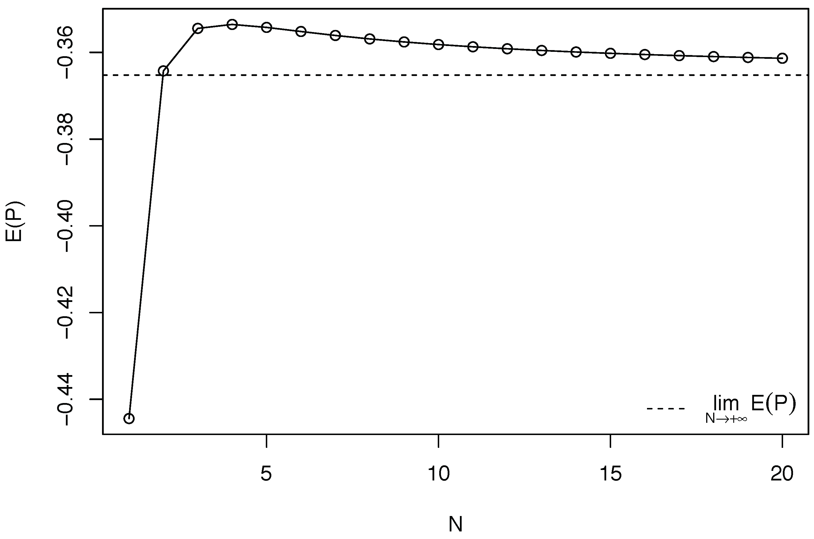
More precisely, the expected performance $\mathbb{E}\left(P\right)$ is single-peaked in the committee size N under the necessary and sufficient condition for the existence of the optimal size. This is immediately shown by the argument in the final paragraph of the proof of Proposition 2. Figure 1 provides a numerical example of this relationship.

The proof of Proposition 2 supports the following argument. When the committee size is small, the positive effect of information aggregation is very strong, and it dominates the negative effect. However, as the committee size becomes larger, the marginal effect of information aggregation becomes weak, and the negative marginal effect due to inefficient information use, the overriding on noisy common information, becomes relatively strong. Thus, the expected performance has a single peak in the committee size. Along the line of the discussion above, I obtain the following characterization of the optimal committee size.

Corollary 2.

Suppose that the parameter set satisfies the necessary and sufficient condition for the existence of the optimal committee size under the average-voting rule: $r>\frac{1}{5}$ and $\frac{\beta }{\omega }<\frac{5r-1}{{(1-r)}^2}$. Then, the optimal size $N^{*}$ is given by the following equation.

$$\begin{array}{c}\hfill N^{*}=\underset{N\in \{N_{-}\left(\tilde{N}\right),N_{+}\left(\tilde{N}\right)\}}{\mathrm{argmax}}\mathbb{E}\left(P\right),\end{array}$$

(18)

where $\tilde{N}\in \mathbb{R}$ is the solution of the equation $f\left(N\right)=\frac{\beta }{\omega }$ with respect to $N\in \mathbb{R}$, $N_{-}\left(\tilde{N}\right)$ is the maximal integer which is not larger than $\tilde{N}$ and $N_{+}\left(\tilde{N}\right)$ is the minimal integer which is not smaller than $\tilde{N}$.

Proof. 

It is obtained immediately from the proof of Proposition 2. □

Note that $\tilde{N}$ depends only on r and the precision ratio $\frac{\beta }{\omega }$ because $\gamma$ and $\frac{\partial \gamma }{\partial N}$ does so: See the necessary part of the proof of Proposition 2. Since $\tilde{N}$ is the single peak of the continuation of $\mathbb{E}\left(P\right)$ with respect to N, $N^{*}$ in (18) is mainly determined by them. However, strictly speaking, $N^{*}$ depends on not the precision ratio but the pair $(\omega ,\beta )$ in general. This is because $\mathbb{E}\left(P\right)$ cannot be written as the function of r and $\frac{\beta }{\omega }$ and it is impossible to decide which of $N_{-}\left(\tilde{N}\right)$ and $N_{+}\left(\tilde{N}\right)$ the optimal size $N^{*}$ is equal to only with the values of r and $\frac{\beta }{\omega }$.

3.3.3. Direction of Strategic Interactions

Although it is straightforward from Proposition 2, the following deserves attention.

Corollary 3.

If $r<0$, then there is no finite optimal size of the committee.

Note that, even in the case of $r<0$, the inefficiency of information use is amplified according to an increase in the committee size. That is, $\gamma$ goes away from the Bayesian weight as the committee size becomes larger. Besides, of course, the marginal positive effect of information aggregation is diminishing. However, in this case, there is no finite optimal size. This is because the inefficiency of the excessive use of private information is absorbed by information aggregation by enlarging committees. This is verified by $\frac{\partial \gamma }{\partial N}f\left(N\right)>0$ in the proof of Proposition 2, which captures the sum of the marginal effects of information aggregation and the excessive dependence on private information.

In contrast, when $r>0$, the excessive use of common information expands, but its inefficiency is not absorbed by information aggregation because the noise term is common to every member. Therefore, in this case, a finite optimal size can exist.

3.4. Comparative Statics

Next, I investigate two relationships between the parameters and the optimal size. Although it is difficult to conduct such comparative statics in analytical ways due to the discreteness of the committee size, I can find the intuitive results below.

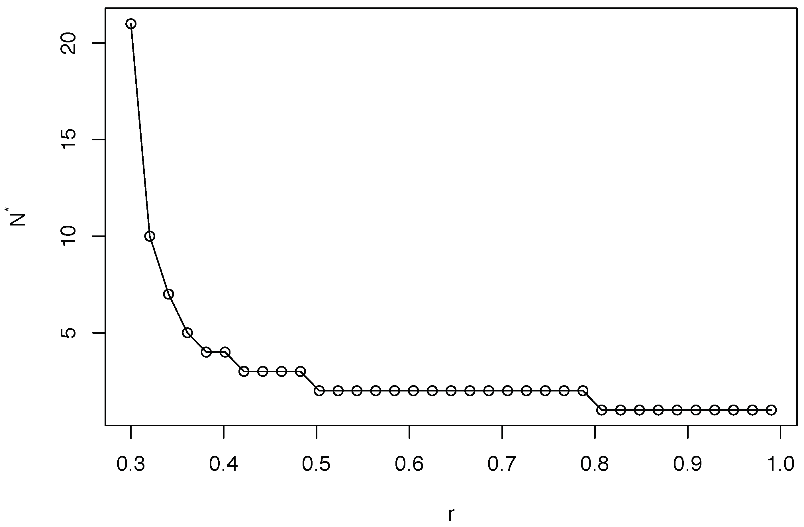
First, I fix $\omega =1.25$ and $\beta =1$, as in Figure 1, and calculate the optimal sizes for various values of r in $[0.3,0.99]$. Figure 2 illustrates the result.

The optimal committee size is non-increasing in the degree of coordination motive, r. When r is small, that is, the motive for conformity is weak, the negative effect of enlarging the committee is small. The importance of enhancing the positive effect of information aggregation is then relatively large. Therefore, the optimal size of the committee is large for small r. As r becomes larger, the optimal size decreases rapidly because the negative effect of conformity acceleratingly swells. Figure 2 provides another interesting fact. It illustrates that the optimal size of the committee is one for sufficiently large r. That is, if the coordination motive is very strong and, hence, adding a committee member is too costly, then a single decision-maker can be optimal.

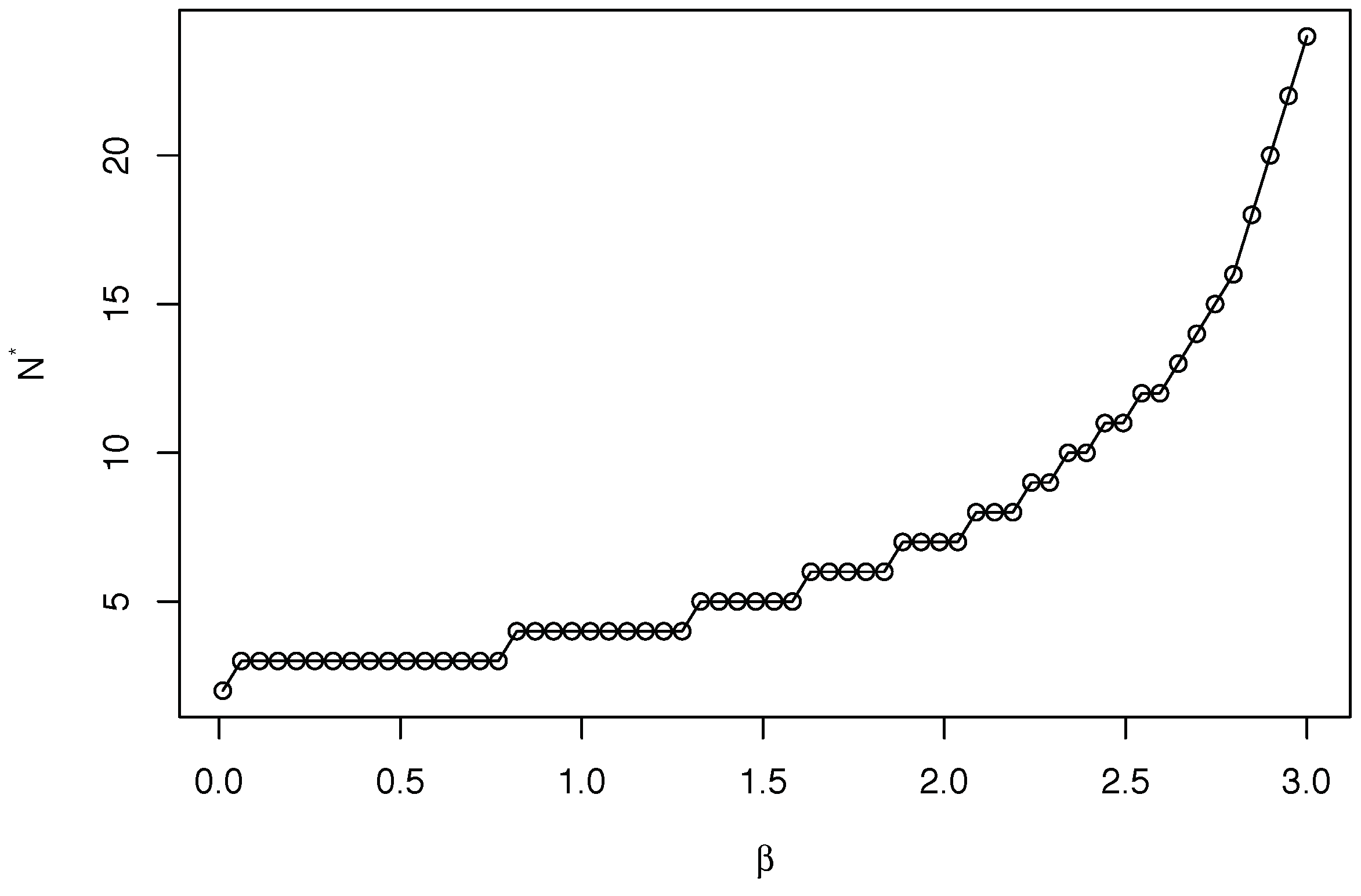
Second, I set $r=0.4$ as in Figure 1 and calculate the optimal sizes for various values of $\beta$ in $[0,3]$ with $\omega$ fixed to 3. Figure 3 illustrates the result.

Given the precision of common information, the optimal committee size is non-decreasing with regards to the precision of private information. Given the degree of coordination motive, when the precision of private information is large relative to that of common information, each member places a high weight on private information. Then, enlarging the committee does not so much foment conformity among the members. The optimal size is, hence, non-decreasing in $\beta$.

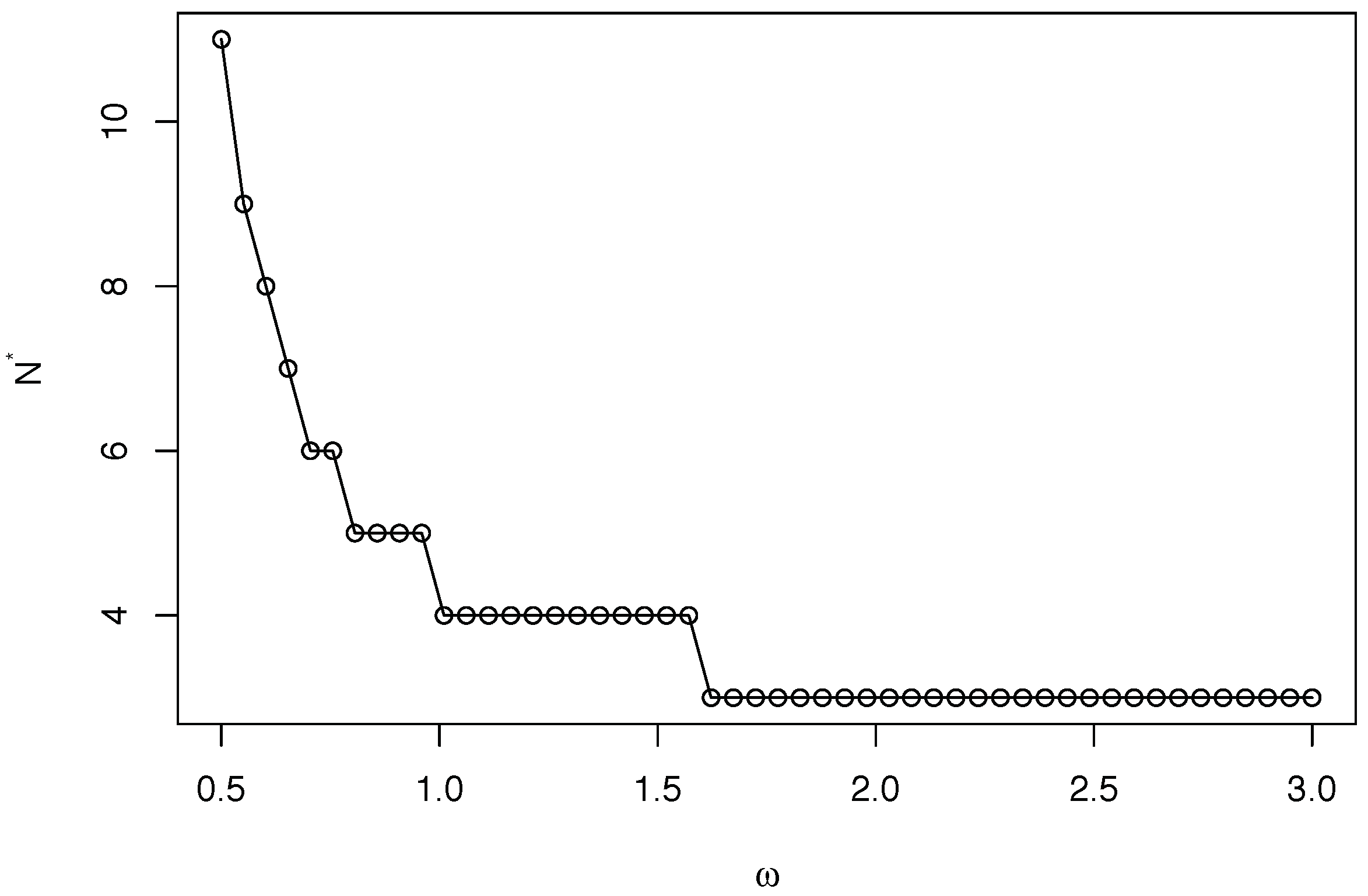
Contrary, such a negative effect of enlarging the committee is strong when the precision of common information is large. Then, the gain of information aggregation is relatively small, and the optimal size is non-increasing in $\omega$; see Figure 4.

The result above suggests that we should establish small committees to reduce the coordination loss when common sense is precise to some extent.

4. Extensions

4.1. Median-Voting Rule

I consider the case where the voting rule is the median-voting rule. The basic properties of the model do not change even under this voting rule. Since each committee member’s behavior is invariant in voting rules, the decision of the committee is

$$\begin{array}{c}\hfill \widehat{a}=\underset{1\le k\le N}{\mathrm{med}}\left\{\gamma x_k\right\}=\gamma \theta +\gamma \underset{1\le k\le N}{\mathrm{med}}\left\{{\epsilon }_k\right\}.\end{array}$$

(19)

Thus, by (5) and (19), I obtain the expected performance of the committee under the median-voting rule:

$$\begin{array}{c}\hfill \mathbb{E}\left(P\right)=-{(1-\gamma )}^2{\omega }^{-1}-{\gamma }^2\mathbb{E}\left[{\left(\underset{1\le k\le N}{\mathrm{med}}\left\{{\epsilon }_k\right\}\right)}^2\right].\end{array}$$

(20)

The expectation in the second term of the right-hand side of (20) has no analytical expression for finite N. However, the distribution of ${\mathrm{med}}_{1\le k\le N}\left\{{\epsilon }_k\right\}$ is approximately the normal distribution with mean 0 and variance $\frac{\pi }{2N}{\beta }^{-1}$ for sufficiently large N: See Kenney and Keeping [30]. Hence,

$$\begin{array}{c}\hfill \mathbb{E}\left(P\right)\approx -{(1-\gamma )}^2{\omega }^{-1}-{\gamma }^2\frac{\pi }{2N}{\beta }^{-1}\end{array}$$

(21)

for sufficiently large N. Thus, by use of the approximation, (21), I obtain a sufficient condition for the existence of the finite optimal committee size under the median-voting rule as follows.

Corollary 4.

Under the median-voting rule, there exists a finite optimal size of the committee if the parameter set satisfies $r>\frac{\pi }{\pi +8}$ and $\frac{\beta }{\omega }<\frac{(\pi +8)r-\pi }{\pi {(1-r)}^2}$.

Proof. 

It is immediately obtained in the same way as the sufficiency part of the proof of Proposition 2. □

Although I refrain from referring to a necessary condition, the basic properties under the average-voting rule would not change because the distribution of sample median approaches that of the sample mean very quickly: See Maritz and Jarret [31]. I cannot find any numerical example for which a finite optimal size exists when the parameter condition does not hold.

The intuition for this sufficient condition is similar to Proposition 2, but there is a quantitative difference between the median-voting rule and the average-voting rule. One can show that the parameter region which satisfies the sufficient condition under the median-voting rule is smaller than that of the average-voting rule. Figure 5 illustrates it.

The cause of this result is the difference between the statistical properties of the mean and median. That is, as seen in ${\mathrm{med}}_{1\le k\le N}\left\{{\epsilon }_k\right\}\propto N(0,\frac{\pi }{2N}{\beta }^{-1})$, sample medians converge in probability more slowly than sample means. Therefore, under the median-voting rule, it is more important to promote the positive effect of information aggregation than under the average-voting rule. This makes the existence condition under the median-voting rule stricter.

4.2. Common Signal

In reality, committee members are usually provided with common signals. For example, members of policy boards receive some staff reports for discussion in formal meetings. Such a common information source can be modeled as a common signal. Here, I assume that each member of the committee receives the following common signal:

$$\begin{array}{c}\hfill y=\theta +\eta ,\end{array}$$

(22)

where $\eta$ follows the normal distribution with mean 0 and variance ${\alpha }^{-1}>0$. Parameter $\alpha$ measures the precision of the common signal. One can investigate the role of such a common signal. By the Bayesian update, each member j’s expectation of $\theta$ with private and common information is

$$\begin{array}{ccc}\hfill {\mathbb{E}}_j\left(\theta \right)& =& \frac{\omega }{(\omega +\alpha )+\beta }\times 0+\frac{\alpha }{(\omega +\alpha )+\beta }y+\frac{\beta }{(\omega +\alpha )+\beta }{x}_j\hfill \\ & =& \frac{\alpha }{(\omega +\alpha )+\beta }y+\frac{\beta }{(\omega +\alpha )+\beta }{x}_j.\hfill \end{array}$$

(23)

Equation (23) reflects that with the common signal, (22), the set of common information consists of the common prior belief (with mean 0 and precision $\omega$) and the common signal (with mean y and precision $\alpha$). It indicates that the case with the common signal is a straightforward extension of the basic model with no common signal. Thus, I only report the results on the equilibrium strategy and the existing condition as follows.

As in Proposition 1, one can conjecture that the equilibrium strategy will be of the form such that

$$\begin{array}{c}\hfill a_j={\gamma }_{c}y+{\gamma }_p{x}_j,\end{array}$$

(24)

where ${\gamma }_c$ and ${\gamma }_p$ are undetermined constants. Using (24), by the same calculation in the proof of the Proposition 1, I obtain the following response coefficients in equilibrium:

$$\begin{array}{ccc}\hfill {\gamma }_c& =& \frac{(1-2\frac{r}{N}+\frac{r}{N^2})\alpha }{(1-r)\beta +(1-2\frac{r}{N}+\frac{r}{N^2})(\omega +\alpha )},\hfill \end{array}$$

(25)

$$\begin{array}{ccc}\hfill {\gamma }_p& =& \frac{(1-r)\beta }{(1-r)\beta +(1-2\frac{r}{N}+\frac{r}{N^2})(\omega +\alpha )}.\hfill \end{array}$$

(26)

Thus, the equilibrium strategy is characterized by (24)–(26).

By the same way as in Proposition 2, one can show that the necessary and sufficient condition for the existence of the optimal committee size is that $r>\frac{1}{5}$ and $\frac{\beta }{\omega +\alpha }<\frac{5r-1}{{(1-r)}^2}$. The intuition for this is the same as that for the case with no common signal. An implication is that the committee should be small when strong conformism exists and the common signal is accurate relative to the private signal.

5. Application: Monetary Policy by Committee

In this section, I provide a simple application of the basic model. Following Morimoto [32] basically, I set up the model for monetary policy analysis which starts from decision-making by the monetary policy committee.

5.1. Macroeconomic Model

As the underlying macroeconomic model, I adopt a basic New Keynesian model. For a brief introduction to the New Keynesian theory, see Galí [33]. The model consists of the two stochastic difference equations:

$$\begin{array}{ccc}\hfill x_t& =& {\mathbb{E}}_t{x}_{t+1}-\frac{1}{\sigma }(i_t-E_t{\pi }_{t+1})+u_t,\hfill \end{array}$$

(27)

$$\begin{array}{ccc}\hfill {\pi }_t& =& \rho {\mathbb{E}}_t{\pi }_{t+1}+\kappa x_t+e_t,\hfill \end{array}$$

(28)

together with a monetary policy rule. Here, $x_t,{\pi }_t,i_t,u_t,e_t$ are output gap, inflation rate, nominal interest rate, demand shock, and cost shock in period t, respectively, and $\rho ,\sigma ,\kappa$ are positive parameters. Parameters $\rho ,\sigma ,\kappa$ represent the discount rate, constant elasticity of intertemporal substitution, and impact of one unit output gap on inflation, respectively.

I assume that $u_t$ and $e_t$ follow identically and independently, the normal distributions with mean zero and variances ${\sigma }_u^2$ and ${\sigma }_e^2$, respectively. Once a set rule of nominal interest rate is specified, macro dynamics of the model economy are determined as sequences of the output gap and inflation rate under the policy rule.

As in most works in optimal monetary policy, I adopt the following social loss function as the welfare measure.

$$\begin{array}{c}\hfill L\equiv V_{\pi }+\lambda V_x,\end{array}$$

(29)

where $V_{\pi }$ and $V_x$ are asymptotic variances of the inflation rate and output gap, and $\lambda$ is the weight that society places on the output gap relative to inflation.

5.2. Interest Rate Setting by Committee

Next, I set up the process of decision-making on interest rate setting in the monetary policy committee. The committee consists of N homogeneous members. The informational structure of the committee is as follows. Each committee member faces information imperfectness about cost shock. For simplicity, I assume that each member can observe the demand shock, $u_t$, because similar results can be obtained if this is relaxed. At the end of period $t-1$, each member receives a private signal on cost shock in period t of the form, such as:

$$\begin{array}{c}\hfill e_t^j=e_t+{\xi }_t^j,\end{array}$$

(30)

where the noise terms of ${\xi }_t^j$ are independently and normally distributed with mean zero and variance ${\sigma }_{\xi }^2$, respectively.

In the meeting of the monetary policy committee, based on her own information, each member j votes the level of nominal interest rate in period t, $i_t^j$, to maximize her own expected payoff. The function form of the payoff function is assumed to be

$$\begin{array}{c}\hfill -r{(i_t^j-i_t^{*})}^2-(1-r){(i_t^j-{\overline{i}}_t)}^2,\end{array}$$

(31)

where $r\in (-1,1)$, ${\overline{i}}_t=\frac{1}{N}{\sum }_{j=1}^N{i}_t^j$, and $i_t^{*}$ is the nominal interest rate in period t set in optimal discretionary policy under perfect information by a single policymaker. That is, $i_t^{*}$ is the solution of the following linear-quadratic problem.

$$\begin{array}{ccc}& min& {\pi }_t^2+\lambda x_t^2,\hfill \\ & \mathrm{s}.\mathrm{t}.& x_t={\mathbb{E}}_t{x}_{t+1}-\frac{1}{\sigma }(i_t-{\mathbb{E}}_t{\pi }_{t+1})+u_t,\hfill \\ & & {\pi }_t=\rho {\mathbb{E}}_t{\pi }_{t+1}+\kappa x_t+e_t.\hfill \end{array}$$

(32)

Here, ${\pi }_t^2+\lambda x_t^2$ is the standard period loss function of the central bank. The control variables are $i_t$, $x_t$, and ${\pi }_t$. The expectational variables, ${\mathbb{E}}_t{x}_{t+1}$ and ${\mathbb{E}}_t{\pi }_{t+1}$, are given in this problem because the policy regime is discretion, in which the central bank does not commit the future economic variations. For a detail explanation of this issue, see Walsh [34]. To solve the problem (32), note that the first constraint, $x_t={\mathbb{E}}_t{x}_{t+1}-\frac{1}{\sigma }(i_t-{\mathbb{E}}_t{\pi }_{t+1})+u_t$, is not binding because it is linear in $i_t$. Thus, the problem is reduced to minimization of ${\pi }_t^2+\lambda x_t^2$ with respect to $x_t$ and ${\pi }_t$ under the constraint ${\pi }_t=\rho {\mathbb{E}}_t{\pi }_{t+1}+\kappa x_t+e_t$. The first order condition is ${\pi }_t=-\frac{\lambda }{\kappa }{x}_t$. Combining this and the constraint ${\pi }_t=\rho {\mathbb{E}}_t{\pi }_{t+1}+\kappa x_t+e_t$, one can obtain $x_t=-\mathsf{\Phi }{e}_t$ and ${\pi }_t=(1-\kappa \mathsf{\Phi })e_t$. Substituting these solution into the constraint $x_t={\mathbb{E}}_t{x}_{t+1}-\frac{1}{\sigma }(i_t-{\mathbb{E}}_t{\pi }_{t+1})+u_t$, I obtain the analytical expression of $i_t^{*}$ such that

$$\begin{array}{c}\hfill i_t^{*}=\sigma (u_t+\mathsf{\Phi }{e}_t),\end{array}$$

(33)

where $\mathsf{\Phi }=\frac{\kappa }{\lambda +{\kappa }^2}$.

Nominal interest rate in period t, $i_t$, is determined by aggregating the voting rates with a specific rule. As the benchmark case, I assume that the voting rule is the arithmetic mean:

$$\begin{array}{c}\hfill i_t=\frac{1}{N}\sum _{j=1}^N{i}_t^j.\end{array}$$

(34)

This is quite simple but sufficient for this paper. In the actual institutions; however, the majority rule is often adopted, hence it being natural to consider the case of the median-voting rule:

$$\begin{array}{c}\hfill i_t=\underset{1\le j\le N}{\mathrm{med}}\left\{i_t^j\right\}.\end{array}$$

(35)

I will show that as in the simple model of the previous sections, the basic result does not change under the median-voting rule.

5.3. Equilibrium Dynamics and Macroeconomic Volatility

Now let us see the equilibrium strategy of the subgame in the committee. By (31), the first order condition of member j’s problem is

$$\begin{array}{c}\hfill i_t^j=(1-\delta ){\mathbb{E}}_{t-1}^j\left(i_t^{*}\right)+\delta {\mathbb{E}}_{t-1}^j\left({\overline{i}}_t\right),\end{array}$$

(36)

where ${\mathbb{E}}_{t-1}^j$ is a mathematical expectation conditioned on information available to member j in the end of period $t-1$, and $\delta$ is defined by (6). Here, by (30) and (33),

$$\begin{array}{c}\hfill {\mathbb{E}}_{t-1}^j\left(i_t^{*}\right)=\sigma (u_t+\mathsf{\Phi }\frac{{\sigma }_{\xi }^{-2}}{{\sigma }_e^{-2}+{\sigma }_{\xi }^{-2}}{e}_t^j).\end{array}$$

(37)

Thus, by use of (36) and (37), I obtain the following proposition immediately from Proposition 1.

Corollary 5.

There exists a unique equilibrium strategy of the form such that

$$\begin{array}{c}\hfill i_t^j=\sigma (u_t+\mathsf{\Phi }{\gamma }_e{e}_t^j),\end{array}$$

(38)

where ${\gamma }_e=\frac{(1-r){\sigma }_{\xi }^{-2}}{(1-r){\sigma }_{\xi }^{-2}+(1-2\frac{r}{N}+\frac{r}{N^2}){\sigma }_e^{-2}}$.

Substituting (38) into (34), I obtain the following equilibrium nominal interest rate.

$$\begin{array}{c}\hfill i_t=i_t^{*}+\sigma \mathsf{\Phi }[-(1-{\gamma }_e)e_t+{\gamma }_e{\overline{\xi }}_t],\end{array}$$

(39)

where ${\overline{\xi }}_t\equiv \frac{1}{N}{\sum }_{j=1}^N{\xi }_t^j$. The second term of (39) represents the inefficiency of interest rate setting due to imperfect information and coordination behavior among the committee members.

The macroeconomic dynamics is given by (27), (28), and (39). Since the relevant state variables in period t are $e_t$ and ${\overline{\xi }}_t$, I can find equilibrium output gap and inflation rate which are linear in them. Thus, noting that ${\mathbb{E}}_t{\pi }_{t+1}={\mathbb{E}}_t{x}_t=0$, one can obtain the following equilibrium output gap and inflation rate.

$$\begin{array}{ccc}\hfill x_t& =& -\mathsf{\Phi }{e}_t-\mathsf{\Phi }[-(1-{\gamma }_e)e_t+{\gamma }_e{\overline{\xi }}_t],\hfill \end{array}$$

(40)

$$\begin{array}{ccc}\hfill {\pi }_t& =& (1-\kappa \mathsf{\Phi })e_t-\kappa \mathsf{\Phi }[-(1-{\gamma }_e)e_t+{\gamma }_e{\overline{\xi }}_t].\hfill \end{array}$$

(41)

The second terms of the equilibrium output gap and inflation rate are the economic fluctuations due to imperfect information and inefficient coordination behavior of the committee. The second term of (41) is $\kappa$ times as large as that of (40). This means that the inefficient interest rate setting brings the inefficient output gap fluctuation, and it hits on inflation through the aggregate supply relation, the New Keynesian Phillips curve.

To find equilibrium social loss, I calculate the variances of the output gap and inflation rate. After some calculations, I obtain

$$\begin{array}{ccc}\hfill V_x& =& {\mathsf{\Phi }}^2{\sigma }_e^2+{\mathsf{\Phi }}^2[{(1-{\gamma }_e)}^2{\sigma }_e^2+{\gamma }_e^2\frac{{\sigma }_{\xi }^2}{N}]-2{\mathsf{\Phi }}^2(1-{\gamma }_e){\sigma }_e^2.\hfill \end{array}$$

(42)

$$\begin{array}{ccc}\hfill V_{\pi }& =& {(1-\kappa \mathsf{\Phi })}^2{\sigma }_e^2+{\kappa }^2{\mathsf{\Phi }}^2[{(1-{\gamma }_e)}^2{\sigma }_e^2+{\gamma }_e^2\frac{{\sigma }_{\xi }^2}{N}]+2(1-\kappa \mathsf{\Phi })\kappa \mathsf{\Phi }(1-{\gamma }_e){\sigma }_e^2.\hfill \end{array}$$

(43)

The first terms of (42) and (43) are due to cost shock, one of the economic fundamentals. The second and third terms are due to the noisiness of private and common information of the committee members, which is one of the non-fundamentals. By (29), (42), (43), and $\mathsf{\Phi }=\frac{\kappa }{\lambda +{\kappa }^2}$, the social loss in equilibrium is reduced to

$$\begin{array}{c}\hfill L=[{(1-\kappa \mathsf{\Phi })}^2+\lambda {\mathsf{\Phi }}^2]{\sigma }_e^2+({\kappa }^2+\lambda ){\mathsf{\Phi }}^2[{(1-{\gamma }_e)}^2{\sigma }_e^2+{\gamma }_e^2\frac{{\sigma }_{\xi }^2}{N}].\end{array}$$

(44)

The social loss L in (44) seems somewhat complicated but its meaning is clear. The first term is equal to the social loss under optimal discretionary policy under perfect information. Since I adopt an optimal policy under discretion as to the optimality concept, the first term is not relevant to the performance of the monetary policy committee. The second term is the social loss generated by the inefficient interest rate setting due to imperfect information and coordination behavior among the members. Therefore, the second term of L should be regarded as the performance measure of the monetary policy committee in this model. Note that it corresponds just to $-\mathbb{E}\left(P\right)$ in the basic model.

5.4. Optimal Size and Positive Implication

5.4.1. Optimal Size of the Monetary Policy Committee

By (44), the optimal size is the size $N\in \mathbb{N}$ which minimizes the following measure of the committee’s loss:

$$\begin{array}{c}\hfill L_{mpc}\equiv {(1-{\gamma }_e)}^2{\sigma }_e^2+{\gamma }_e^2\frac{{\sigma }_{\xi }^2}{N}.\end{array}$$

(45)

Note that, by (45), minimization of $L_{mpc}$ is the same problem as maximization of $\mathbb{E}\left(P\right)$ in the basic model. Thus, immediately from Proposition 2 and Corollary 4, I obtain the result on the optimal size of the monetary policy committee.

Corollary 6.

(i)

Under the average-voting rule (34), there exists a finite optimal size of the monetary policy committee if and only if $r>\frac{1}{5}$ and $\frac{{\sigma }_{\xi }^{-2}}{{\sigma }_e^{-2}}<\frac{5r-1}{{(1-r)}^2}$.

(ii)

Under the median-voting rule (35), there exists a finite optimal size of the monetary policy committee if $r>\frac{\pi }{\pi +8}$ and $\frac{{\sigma }_{\xi }^{-2}}{{\sigma }_e^{-2}}<\frac{(\pi +8)r-\pi }{\pi {(1-r)}^2}$.

The properties of the optimal size of the monetary policy committee are the same as those of the basic model. Therefore, I do not report numerical examples here. First, the optimal size $N^{*}$ is non-increasing in r. That is, the stronger whatever foments the coordination behavior among the committee members is, the smaller the monetary policy committees should be. From the standpoint mentioned above, it is optimal to promote efficient use of the members’ information by keeping the monetary policy committee small. Second, consider an extended model in which a common signal on $e_t$ exists. By the calculation above, it is obvious that the result from this extended model is the same as that of the model in Section 4.2. Thus, in this model, given the precision of private information, the optimal size is non-increasing in the precision of common information. In the context of the monetary policy committee, this is interpreted that the committee size should be small when the staff report or common understanding of general economists on economic states is reliable to some extent.

5.4.2. A Positive Implication

Finally, I mention a positive implication of the model for the actual monetary policy committees. Using a data set on the characteristics of the monetary policy committees in more than 30 countries from 1960 through 2000, Berger and Nitsch [28] report that inflation volatility is U-shaped in the size of the monetary policy committee. In the present paper, by (43), the inflation volatility exhibits similar behavior. In fact, consider the case of $r>0$. Then, differentiating $V_{\pi }$ in (43) with respect to N, I obtain

$$\begin{array}{c}\hfill \frac{\partial V_{\pi }}{\partial N}=\underset{>0}{\underbrace{-2{\sigma }_e^2\frac{\partial {\gamma }_e}{\partial N}(1-\kappa \mathsf{\Phi }{\gamma }_e)}}+\underset{<0}{\underbrace{\kappa \mathsf{\Phi }(2{\gamma }_e\frac{\partial {\gamma }_e}{\partial N}\frac{{\sigma }_{\xi }^2}{N}-{\gamma }_e^2\frac{{\sigma }_{\xi }^2}{N^2})}},\end{array}$$

(46)

where $\frac{\partial {\gamma }_e}{\partial N}<0$ for $r>0$ as in the basic model and $\kappa \mathsf{\Phi }{\gamma }_e=\frac{{\kappa }^2}{\lambda +{\kappa }^2}{\gamma }_e<1$. Equation (46) suggests that inflation variability can be U-shaped with respect to the committee size when there is not only stabilization by information aggregation (the second term) but also inefficient information use due to coordination (the first term).

6. Discussion

In this paper, the coordination motive among the members generates the trade-off of enlarging the committee and the existence of a finite committee size. This is in the line of the literature on transparency and economic behavior: Prat [4], Levy [7,8], Meade and Stasavage [9], Hansen et al. [10], Fehrler and Hughes [6].

One can consider another source of such a coordination behavior in collective choice. Depending on environments, conformism can bring a tangible benefit for members of organizations. For example, some rewards are delivered substantially for workers when their opinions are similar to their manager’s one: Prendergast [35]. In this case, the workers are incentivized to coordinate with the average, and the information gathering in the organization is distorted. Tug-of-wars in organizations, such as political parties, have the similar mechanism. When a member’s individual choice is close to a party’s final decision, she obtains advantage in the party after that. This leads to conformity and overriding on common information.

Therefore, in addition to overcoming the fault of costly information acquisition approach, the approach of the present paper has plenty of contexts which are studied in economics of organizations. I think that some potential applications of interest exist. For instance, the mechanism in this paper should be applied to microeconomics of firms’ affairs and political science, as well as the optimal size of monetary policy committees.

However, this study has some limitations. It is difficult to observe the preferences for coordination, although I assume that there is no preference uncertainty in the model. We face a problem of ex-post manipulations of voting under preference uncertainty, but the analysis of this paper provides a key to solve it. As Figure 1 illustrates, the expected performances of the oversized committees dominate those of the undersized committees. This indicates that the optimal size of committees will increase by incorporating preference uncertainty. That is, enlarging the committee mitigates the loss of preference uncertainty. In applications, interactions of the committee size and other specific factors can be considered. For example, in the field of monetary policy design, there are existing studies which incorporate preference uncertainty: Beetsma and Jensen [36]. In particular, Morimoto [37] considers the case where the committee with uncertain preferences conducts monetary policy, and solves the optimal delegation problem of monetary policy committees under preference uncertainty in inflation targeting. I think it will be interesting to consider the uncertainty about the preference for coordination in the models of monetary policy committees in future works.

Another limitation is that this paper does not consider communication among the members. Although complex communication structures would not be theoretically tractable, one can analyze pairwise communication in a network structure; see Calvó-Armengol and de Martí Beltran [38]. Because communication in a network affects the information gathering and welfare in organizations, its applications to the issues of the Condorcet jury theorem will be of interest.

7. Conclusions

This paper explores the determination of optimal committee sizes, focusing on coordination behavior among the members with higher-order beliefs. Contrary to incorporating information acquisition costs, which is usually adopted in literature, the optimal size in this paper’s model is directly determined by the wedge of the equilibrium behavior. This paper also analyzes in a formal model the optimal size of monetary policy committees, which is one of the most important and difficult issues of contemporary monetary policy design.

There are a few remaining problems. The first one is to construct models with theoretical foundations for the members’ coordination motive. It seems very significant in the area of committee design. In particular, I think transparency and reputation can play an important role for it as some studies argue. The second one is to find applications of the mechanism given in this paper to other economic problems. Considering the structure of this paper’s model, the mechanism will apply to the models in which the optimal action of the committee under perfect information is a linear function of states. I believe that such situations are not rare in the economic phenomena of our interest.

References

- Condorcet, M. Essai sur L’application de L’analyse á la Probabilité des Decisions Rendues a al Pluralité de Voix; L’Imprimerie Royale: Paris, France, 1785. [Google Scholar]
- Li, H. A theory of conservatism. J. Polit. Econ. 2001, 109, 617–636. [Google Scholar] [CrossRef]
- Gerling, K.; Grüner, H.P.; Kiel, A.; Schulte, E. Information acquisition and decision making in committees: A survey. Eur. J. Polit. Econ. 2005, 21, 563–597. [Google Scholar] [CrossRef] [Green Version]
- Prat, A. The wrong kind of transparency. Am. Econ. Rev. 2005, 95, 862–877. [Google Scholar] [CrossRef] [Green Version]
- Visser, B.; Swank, O. On committees of experts. Q. J. Econ. 2007, 122, 337–372. [Google Scholar] [CrossRef]
- Fehrler, S.; Hughes, N. How transparency kills information aggregation: Theory and experiment. Am. Econ. J. Microecon. 2005, 10, 181–209. [Google Scholar] [CrossRef] [Green Version]
- Levy, G. Anti-herding and strategic consultation. Eur. Econ. Rev. 2004, 48, 503–525. [Google Scholar] [CrossRef] [Green Version]
- Levy, G. Decision making in committees: Transparency, reputation, and voting rules. Am. Econ. Rev. 2007, 97, 150–168. [Google Scholar] [CrossRef] [Green Version]
- Meade, E.; Stasavage, D. Publicity of debate and the incentive to dissent: Evidence from the US Federal Reserve. Econ. J. 2008, 118, 695–717. [Google Scholar] [CrossRef]
- Hansen, S.; McMahon, M.; Prat, A. Transparency and deliberation with the FOMC: A computational linguistics approach. Q. J. Econ. 2018, 133, 801–870. [Google Scholar] [CrossRef] [Green Version]
- Muto, T. How do central banks make decisions?: Monetary policy by committee. In Proceedings of the Summary of the Spring Meeting of the Japan Society of Monetary Economics, Chiba, Japan, 12 May 2007. [Google Scholar]
- Blinder, A. Monetary policy by committee: Why and how? Eur. J. Polit. Econ. 2007, 23, 106–123. [Google Scholar] [CrossRef] [Green Version]
- Austen-Smith, D.; Banks, J.S. Information aggregation, rationality, and the Condorcet jury theorem. Am. Polit. Sci. Rev. 1996, 90, 34–45. [Google Scholar] [CrossRef] [Green Version]
- Feddersen, T.; Pesendorfer, W. Voting behavior and information aggregation in elections with private information. Econometrica 1997, 65, 1029–1058. [Google Scholar] [CrossRef]
- Feddersen, T.; Pesendorfer, W. Convicting the innocent: The inferiority of unanimous jury verdicts under strategic voting. Am. Polit. Sci. Rev. 1998, 92, 23–35. [Google Scholar] [CrossRef]
- Persico, N. Committee design with endogenous information. Rev. Econ. Stud. 2004, 71, 165–191. [Google Scholar] [CrossRef]
- Martinelli, C. Would rational voters acquire costly information? J. Econ. Theory. 2006, 129, 225–251. [Google Scholar] [CrossRef] [Green Version]
- Mukhopadhaya, K. Jury size and the free rider problem. J. Law Econ. Organ. 2003, 19, 24–44. [Google Scholar] [CrossRef]
- Koriyama, Y.; Szentes, B. A resurrection of the Condorcet jury theorem. Theor. Econ. 2009, 4, 227–252. [Google Scholar]
- Cai, H. Costly participation and heterogeneous preferences in informational committees. RAND J. Econ. 2009, 40, 173–189. [Google Scholar] [CrossRef]
- Gerardi, D.; Yariv, L. Information acquisition in committees. Games Econ. Behav. 2008, 62, 436–459. [Google Scholar] [CrossRef] [Green Version]
- Oliveros, S. Abstention, ideology and information acquisition. J. Econ. Theory. 2013, 148, 871–902. [Google Scholar]
- Großer, J.; Seebauer, M. The curse of uninformed voting: An experimental study. Games Econ. Behav. 2016, 97, 205–226. [Google Scholar] [CrossRef] [Green Version]
- Bhattacharya, S.; Duffy, J.; Kim, S. Voting with endogenous information acquisition: Experimental evidence. Games Econ. Behav. 2017, 102, 316–338. [Google Scholar] [CrossRef] [Green Version]
- Mechtenberg, L.; Tyran, J.-R. Voter motivation and the quality of democratic choice. Games Econ. Behav. 2019, 116, 241–259. [Google Scholar] [CrossRef] [Green Version]
- Elbittar, A.; Gomberg, A.; Martinelli, C.; Palfrey, T. Ignorance and bias in collective decisions. Games Econ. Behav. 2020, 174, 332–359. [Google Scholar] [CrossRef] [Green Version]
- Sibert, A. Central banking by committee. Int. Financ. 2006, 9, 145–168. [Google Scholar] [CrossRef]
- Berger, H.; Nitsch, V. Too many cooks? Committees in monetary policy. South. Econ. J. 2011, 78, 452–475. [Google Scholar] [CrossRef]
- Morris, S.; Shin, H.S. Social value of public information. Am. Econ. Rev. 2002, 92, 1521–1534. [Google Scholar] [CrossRef] [Green Version]
- Kenney, J.F.; Keeping, E.S. Mathematics of Statistics, Part 2; Van Nostrand: Princeton, NJ, USA, 1962. [Google Scholar]
- Maritz, J.S.; Jarrett, R.G. A note on estimating the variance of the sample median. J. Am. Stat. Assoc. 1978, 73, 194–196. [Google Scholar] [CrossRef]
- Morimoto, K. Optimal Structure of Monetary Policy Committees; Discussion Papers in Economics and Business, 09-36-Rev; Graduate School of Economics, Osaka University: Osaka, Japan, 2009. [Google Scholar]
- Galí, J. Monetary Policy, Inflation, and the Business Cycle: An Introduction to the New Keynesian Framework and its Applications, 2nd ed.; Princeton University Press: Princeton, NJ, USA, 2015. [Google Scholar]
- Walsh, C. Monetary Theory and Policy, 4th ed.; MIT Press: Cambridge, MA, USA, 2017. [Google Scholar]
- Prendargast, C. A theory of “yes men”. Am. Econ. Rev. 1993, 83, 757–770. [Google Scholar]
- Beetsma, R.; Jensen, H. Inflation targets and contracts with uncertain central banker preferences. J. Money Credit Bank. 1998, 30, 384–403. [Google Scholar] [CrossRef]
- Morimoto, K. Further results on preference uncertainty and monetary conservatism. Econ. Bull. 2018, 38, 583–592. [Google Scholar]
- Calvó-Armengol, A.; de Martí Beltran, J. Information gathering in organizations: Equilibrium, welfare, and optimal network structure. J. Eur. Econ. Assoc. 2009, 7, 116–161. [Google Scholar] [CrossRef] [Green Version]
Figure 1.
The relationship between committee size and expected performance (, , ).
Figure 2.
The relationship between degree of coordination motive and optimal size (, ).
Figure 3.
The relationship between precisions of private signals and optimal size (, ).
Figure 4.
The relationship between precisions of common information and optimal size (, ).
Figure 5.
The regions below the blue and red curves are the parameter regions that satisfy the sufficient conditions for the existence of optimal committee size under the average and median voting rules, respectively. The former contains the latter.
Publisher’s Note: MDPI stays neutral with regard to jurisdictional claims in published maps and institutional affiliations. |
© 2021 by the author. Licensee MDPI, Basel, Switzerland. This article is an open access article distributed under the terms and conditions of the Creative Commons Attribution (CC BY) license (https://creativecommons.org/licenses/by/4.0/).
Share and Cite
MDPI and ACS Style
Morimoto, K. Information Use and the Condorcet Jury Theorem. Mathematics 2021, 9, 1098. https://doi.org/10.3390/math9101098
AMA Style
Morimoto K. Information Use and the Condorcet Jury Theorem. Mathematics. 2021; 9(10):1098. https://doi.org/10.3390/math9101098
Chicago/Turabian StyleMorimoto, Keiichi. 2021. "Information Use and the Condorcet Jury Theorem" Mathematics 9, no. 10: 1098. https://doi.org/10.3390/math9101098
Note that from the first issue of 2016, this journal uses article numbers instead of page numbers. See further details here.