Smooth kNN Local Linear Estimation of the Conditional Distribution Function


1
Department of Mathematics, College of Science, King Khalid University, Abha 62529, Saudi Arabia
2
Statistical Research and Studies Support Unit, King Khalid University, Abha 62529, Saudi Arabia
3
AGIM Team, Laboratoire AGEIS, EA 7407, Université Grenoble Alpes (France), UFR SHS, BP. 47, CEDEX 09, F38040 Grenoble, France
*
Author to whom correspondence should be addressed.
Mathematics 2021, 9(10), 1102; https://doi.org/10.3390/math9101102
Submission received: 1 April 2021
/
Revised: 9 May 2021
/
Accepted: 10 May 2021
/
Published: 13 May 2021
(This article belongs to the Section Probability and Statistics)
Abstract
:Previous works were dedicated to the functional k-Nearest Neighbors (kNN) and the local linearity method estimations of a regression operator. In this paper, a sequence pair of of functional mixing observations are considered. We treat the local linear estimation of the cumulative function of given functional input variable . Precisely, we combine the kNN method with the local linear algorithm to construct a new and fast efficiency estimator of the conditional distribution function. The main purpose of this paper is to prove the strong convergence of the constructed estimator under mixing conditions. An application to the functional times series prediction is used to compare our proposed estimator with the existing competitive estimators, and show its efficiency and superiority.
1. Introduction
In the last decade, the local linearity method (LLM) estimation has become an interesting growing method in nonparametric Functional Data modeling (NPFDM). This topic’s motivation is the superiority of LLM-estimation over the method of the classical kernel weighting method (CKM). Especially, the CKM has a large bias compared to the LLM-estimation (see Fan and Gijbels [1] for a uni-dimensional framework, and Baìllo and Grané [2] for NPFDM setup). Baìllo and Grané [1] used the LLM-algorithm to estimate the hilibertian conditional expectation operator. A generalized LLM-estimation of this nonparametric operator was obtained by Barrientos et al. [3]. They treated the case of Banach explanatory variable. Berlinet et al. [4] built an alternative LLM-estimator of the functional conditional expectation by inverting the local variance-covariance matrix of the functional variable. The asymptotic distribution of the LLM-estimator proposed by Barrientos et al. [3] was obtained by Zhou and Lin [5].
Furthermore, the LLM-estimation of the conditional cumulative distribution function (CCDF) was investigated by Laksaci et al. [6], who established the almost consistency rate for an LLM-estimator of the CCDF-model when the observations have spatio-functional structure. All these previous studies have utilized the kernel local linearity method; however, this paper focuses on CCDF-estimation with a new weighting approach obtained by mixing the local linear fitting to the kNN method.
1.1. Related Works
Recall that the estimation by kNN method has more advantages than the Nadaraya-Watson algorithm. It is an attractive procedure of estimation which is more acclimated to the functional formation of underlying data (see Burba et al. [7] for more motivations on this approach). Notice also that the method of kNN, in the nonparametric functional statistic, has been studied by many researchers (see, for instance, Laloë [8], Kudraszow and Vieu [9] for previous works and Kara et al. [10] for the uniform consistency on the number of neighbors). On the other hand, the kNN estimation under the local linear approach was recently developed by Chikr-Elmezouar et al. [11]. They constructed an estimator of the conditional density by combining the ideas of the local linear method to the kNN weighting techniques. They proved the almost complete consistency of the constructed estimator when the observations are independent identically distributed. Considering the same situation for functional observations in the case of independent identically distributed, Bachir et al. [12] have studied the estimation of the M-regression function. Their estimator was obtained using the kNN approach over the Nadaraya-Watson method. They established the convergence rate of the uniform consistency on the number of the neighbor of the constructed estimator. As an alternative model to the robust regression, Laksaci et al. [13] have treated the kNN estimation of the quantile regression. They stated the property of the built estimator under the independence structure. We refer to Rachedi et al. [14] for the functional regression when the response variable is observed with missing data at random. More recently, Almanjahie et al. [15] have studied the computational aspects of the kNN estimation of some nonparametric functional models, including the conditional density, the regression operator, and the conditional cumulative function. They examined the feasibility of some selector algorithms to choose the best bandwidth parameter in nonparametric functional data analysis.
1.2. Contribution
While the previous works are dedicated to the functional kNN-estimation of the regression operator using the CKM-method, we consider, in this contribution, the kNN estimation problem of the CCDF using the LLM-smoothing. Precisely, we benefit from the attractive features of both the kNN weighting and LLM-fitting by combining the two algorithms to provide a fast efficiency estimator for the CCDF. On the one hand, it is well known that the main reason behind the implementation of the kNN method is its feature to select an attractive smoothing parameter. Specifically, the kNN method permits the selection of a bandwidth parameter more adapted to the local structure of the data. Moreover, this estimator can be updated to any new observations. Such consideration is essential in functional statistics where the asymptotic properties are strongly dependent on the behavior of the local structure. For the latter reason, the kNN method is better than the classical kernel method. However, the difficulty in the kNN smoothing is the fact that the bandwidth parameter is a random variable, unlike the kernel method in which the smoothing parameter is a deterministic scalar. So, the study of the asymptotic properties of this estimator is complicated, and it requires some additional tools and techniques.
On the other hand, it is well documented that the local linear approach is an alternative method to the usual Nadaraya-Watson technique. As discussed in the first paragraph, the estimation by local linear method permits to improve the asymptotic property of the kernel estimator by reducing the bias term. Thus, with this combined approach, we construct an estimator of the CCDF and state their consistency by establishing the almost complete convergence rate. The second novelty of this contribution is establishing the asymptotic results of the estimator when the observations are correlated as mixing functional time series.
1.3. Organization
This paper is structured as follows. Our Methodology describing the kNN-LLM estimator, as well as the functional time series framework, is presented in Section 2. The main asymptotic results with their proofs are also presented in Section 3. Section 4 is devoted to some comments allowing to reveal the very merits of the proposed approach. The performance of the constructed estimator in temperature prediction, compared to existing estimator, using real data is conducted in Section 5. Our conclusion is presented in Section 6.
2. Methodology
2.1. CCDF-Model and Its kNN-LLM Estimator
Consider be stationary sequence of random vector valued in , where is a separable metric space has a metric d. Let be the neighborhood of fixed curve , for which we suppose that the conditional cumulative distribution function (CCDF) has a continuous conditional density . Usually, the LLM-estimator of CCDF is built by treating the function as a conditional expectation, i.e.,
where H is the cumulative distribution function, and is a positive real sequence. In fact, this idea was proposed, first, by Fan and Gijbels [1] in nonfunctional setup. In our functional context, we consider an alternative estimator to that proposed by Almanjahie et al. [16]. It is obtained by approximating locally in by
So, the kNN-LLM estimator is constructed by estimating the operators and of the formula in (1) as
where is a kernel function, , and . Then, we prove, later, that the smooth kNN-LLM of the CCDF is explicited by
where
2.2. Functional Time Series Framework
We study the behavior of asymptotic property of the LLM-estimator based on CCDF when the data is observed as functional time series (FTS). It should be noticed that the functional time series analysis has been widely developed in the area of functional statistics; see Ferraty and Vieu [17] for an important discussions. In this paper, we carry out our functional time series framework by assuming that the sequence is algebraic -mixing has coefficient of mixing such that
As for all asymptotic results, in nonparametric functional statistic, we need to control the local concentration of both marginal and joint distributions of the functional observations. Indeed, for the mariginal distribution, we assume that
such that
For the joint distribution, we assume that
where refers to a ball with a center x and a radius h.
The challenging aim of the paper is to establish the convergence rate of the kNN-LLM estimator without independence assumption. Of course, this general consideration requires different tools to those used for the independent situation. In the rest of this section, we give the necessary background to handle this situation.
Lemma 1
(see Ferraty and Vieu [17]). Let be an algebraic α-mixing process which is identically distributed.
- 1.
- If there exist and such that, for all , then, for all , , we have
- 2.
- If there exists such that , then, for all and :where .
3. Results: The Asymptotic Properties of the kNN-LLM Estimator of CCDF
Now, we prove the a.co. convergence of the estimator toward . Firstly, let us point out that the condition (4) ensures the existence of that satisfies
So, in the remainder of this paper, we put , , and . Next, to establish the convergence rate of our estimator, we set the following conditions.
The kernel is differentiable function and has support . Moreover, its first derivative exists and ∃ C and satisfy
and for ,
The conditional distribution function satisfies, for all and ,
The sequence
satisfies that
Remark 1.
The conditions (6)–(8) are quite weak in time series analysis. Indeed, we point out that most of the conditions are similar to the previous works in functional time series. On the other hand, similar conditions to (6) and (8) can be also found in Ferraty and Vieu [17]. A deeper and clear discussion on the generality of our framework is given in the next Section.
Theorem 1.
Proof of Theorem 1.
The details of the proof is given in the Supplementary File. It is based on the following Lemmas. □
Lemma 2.
Using the same conditions of Theorem 1, we have
where
Lemma 3.
Using the same conditions of Theorem 1, we have
where,
In the following, we will show the mathematical proofs of the above intermediate results. When no ambiguity is possible, C and will be used to denote some strictly positive generic constants with .
Proof of Theorem 2.
The proof is based on the exponential inequality of the Fuck-Nagaev (see Lemma 1) on
Since
it follows that, for all , we obtain
where
For a suitable choice of and by (8), we get
□
Proof of Theorem 3.
Once again, as in Lemma 2’s proof, we apply the exponential inequality of Fuck-Nagaev for another random variables as
Since
we get
which allows to write
This last achieves the proof of this lemma. □
4. Discussions and Comments
4.1. The kNN Method in Functional Statistics
Motivated by its flexibility in practice, the kNN-method is becoming a popular nonparametric data analysis. It was introduced in functional statistics by Burba et al. [7]. The implementation of this approach in functional data analysis is promising. Indeed, as with all nonparametric smoothing approaches, the kNN method has some drawbacks in multivariate analysis, such as its high sensitivity to feature vectors, the slowness of the execution-time when the data has large volume, or the excessive use of the memory. It is well known that all these drawbacks are due to the problem of the curse of dimensionality in vectorial statistics. This problem was handled by using the small probability function to evaluate the asymptotic property of the estimator. Indeed as discussed in Ferraty et al. [7] the small probability function quantifies the concentration property of the probability measure of the functional variable, and it has an inherent role in functional data analysis. In a sense that a less concentration of the probability measure of the functional variable implies a slower rate of convergence of the estimator. Then, the best way of resolving the above drawbacks is to increase the concentration of the functional variable in neighbor of the location point x. To do that, we use the fact that the small ball probability function depends crucially on the metric . Hence, from a statistical point of view, we can increase the concentration property by choosing the best metric d. Thus, we can say that the implantation of the kNN in functional data analysis is very beneficial in practice, and their drawbacks of the multivariate can be overcome by using the appropriate topological structure.
4.2. On the Impact of This Contribution
It is well known that the conditional distribution function has a pivotal role in nonparametric statistics modeling. Indeed, the nonparametric estimation of this model is an imperative step for various nonparametric models, such as conditional density, the conditional hazard, and the conditional quantile functions. The conditional cumulative distribution function in the prediction setting allows to construct many predictive intervals or, more generally, predictive regions. We mention, for instance, the conditional percentile interval, the shortest conditional modal interval (SCMI), and the maximum conditional density region (MCDR) (see Yao and Tong [18] for their definitions). Of course, the diversity of the applicability of the conditional distribution function highlights the importance of this conditional model, which has the advantage of completely characterizing the conditional law of the considered random variables. As mentioned in the bibliographical discussion of the introduction’s section, this model has been widely studied in nonparametric functional statistics. However, the novelty of the present contribution is mainly the estimation of this model by combining two important approaches: the local linear method and the k-Nearest Neighbors procedure. This combination allows to construct a new attractive estimator that inherits the advantages for both methods. Indeed, it is well known that the local linear method improves the bias property of the kernel method, while the weighting by the kNN algorithm offers a sophisticated procedure for the smoothing parameter selection. It is locally selected with respect to the vicinity at the conditioning point, which permits to construct an adaptive estimator to the data’s local structure. Such consideration is very important in (nonparametric functional data analysis, where the performance of estimators is closely linked to the local structure of the data through concentration properties of the probability measure (see Ferraty and Vieu [17]). Nevertheless, the establishment of the asymptotic properties of this estimator is more difficult than the classical case studied by Laksaci et al. [6] because, here, the bandwidth parameter is a random variable, unlike the standard case where the bandwidth parameter is a scalar. Considering the dependent case, which is a more general and more realistic situation, this difficulty becomes more complicated. We can say that the principal axes of this contribution are (1) the conditional distribution function as a pivotal model for various nonparametric conditional models, (2) the estimation method as a new proceeder even in the nonfunctional case (as far as we know, there is no work in the CCDF estimation by combining the LLE to kNN) and (3) the functional time series case as a generalization of the independent case. To emphasize the usefulness of the present contribution in the prediction issue, we discuss in the following section how we can predict future real characteristics of a continuous-time process given its past.
4.3. Some Particular Cases
One of the main features of the present work is treating the kNN-local linear estimation under the dependent case. The latter allows for regrouping several usual situations. To highlight the importance and the generality of the present contribution, we come back to particularize our study for these usual situations. In particular, we consider the independent case, the strong local dependency case, and the local constant method. Let us note that, for the sake of brevity, detailed proof of the corollaries is given in the Supplementary File.
- The independent case: The independent case is widely studied in the past for some alternative models. However, this case can be treated as a particular case for this contribution. It corresponds to the case of . In this situation, the condition (2) is automatically stratified, and Theorem 1 leads straightforwardly to the following Corollary.Corollary 1.We point out that this result is also new as the kNN-LLM estimator of the CCDF in the i.i.d. case.
- The strong local dependency: The second particular case is the case when the local dependency, measured by , is of orderThen, in this situation, the Theorem 1 is reformulated as follows. Obviously, the convergence rate of this particular case is more speed than the general form given in Theorem 1.
- The local constant method: It is well known that the Nadaraya-Watson estimator can be viewed as a particular case of the local linear approach. It can be obtained by taking . This case is so-called local constant approach and its kNN estimator is defined byThis estimator has been studied by Karra et al. [10]. They established its asymptomatic properties when the observations are independent identically distributed. While, here, we develop the dependent case. Once again, the kNN-LCM estimator’s consistency is also new in this context of nonparametric functional data analysis. It is given in the following corollary.
5. Real Data Applications
5.1. Application to Functional Time Series Prediction
One of the main feature of the CCDF is the possibility to construct several predictive regions . Of course, the efficiency of each prediction interval is assessed by the means of the length of the set and the presence of the true value in . It is well documented that the width of the SCMI is the smallest compared to all predictive regions with the same coverage probability. It was introduced by Yao and Tong [18] and obtained by
The refers to the Lebesgue measure. Using the CCFD estimators, we approximate the SCMI by
5.2. Example 1: Application to Climatological Time Series Data
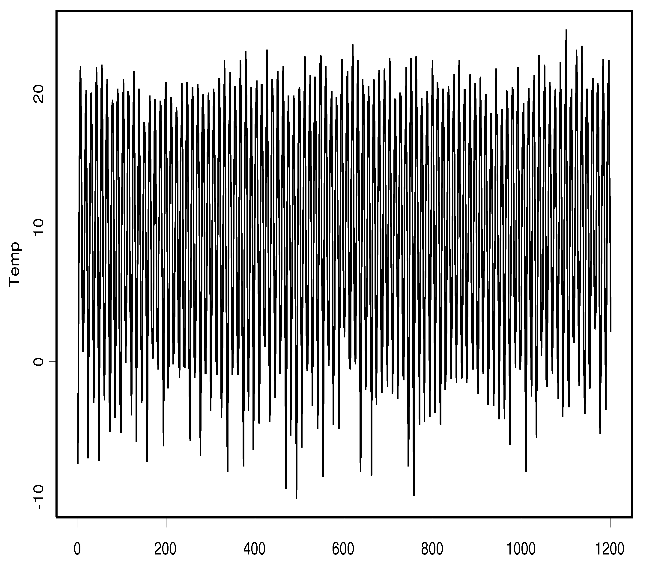
In this first example, we show the applicability of the proposed estimators to climatological data. Indeed, we predict the monthly average temperature one year ahead in Debrecen’s station in Hungary. The link to the data is provided in the “Data Availability Statement” section. Let us note that the studied data is recently collected, and it contains only some missing values, which are replaced by the average of the values before and after the analyses. Now, from this observed data, we construct curves , where denotes the average temperature curve observed during the (1 year) 12 months of the i-th year. The observed data are plotted in Figure 1, representing the values of the monthly average of the temperature.
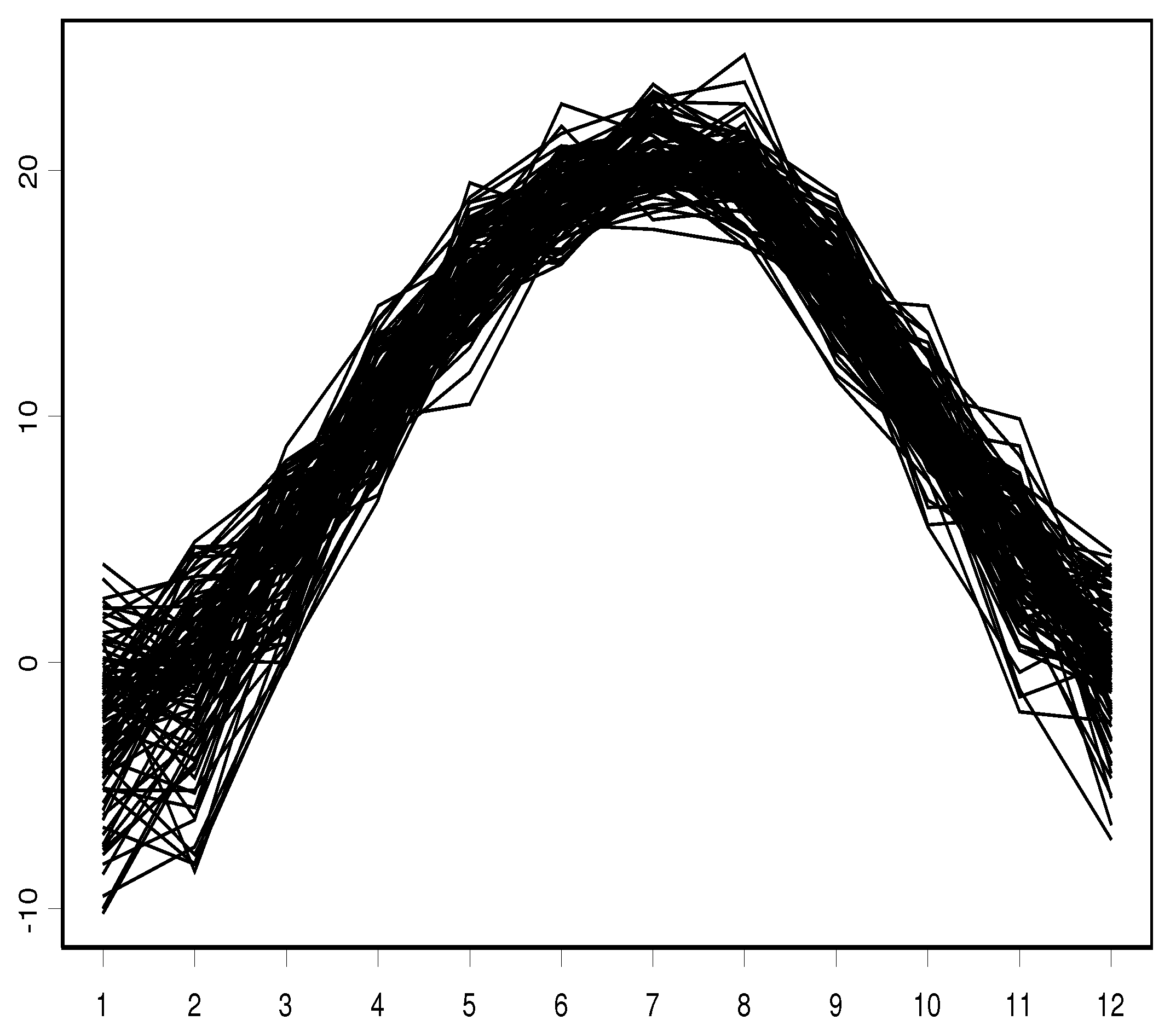
In Figure 2, we plot the that represents the yearly curves of the temperature.
The efficiency of the SCMI predictive interval is linked to the parameters’ choices in the estimator . For this computational purpose, we compute with the quadratic kernel K. The metric d is determined according to the PCA-algorithm. In this application part, we shall compare the predictive interval (SCMI ) using the kNN-LLM estimator instated to the CKM-estimator studied by Laksaci et al. [6]. In both estimators, we choose k and h by the same cross-validation method used by De Gooijer and Gannoun [19], which is based on the following criterion:
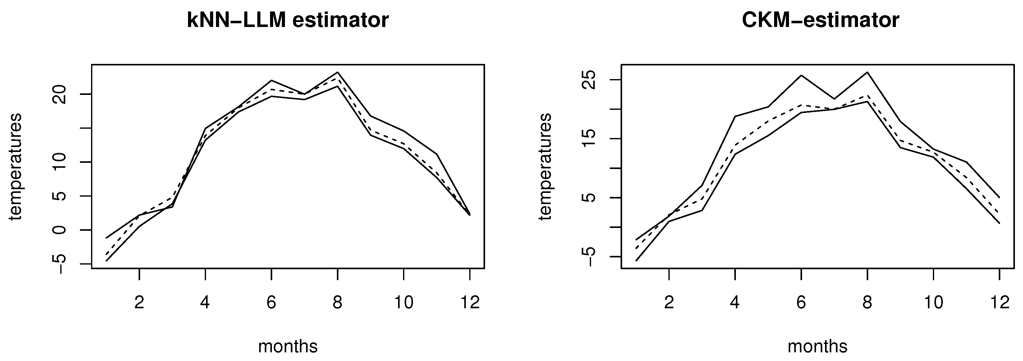
Now, the SCMI predictive interval of the whole curve of the last year () of this sample knowing the functional covariates , by commuting , where is the nearest curve to using the learning sample with , for each fixed month . Figure 3 displays the results where we plot three curves: The true curve in the dashed line and the extremities of the SCMI- interval are given in the continuous line.
The observed data is displayed in the dashed curve and the solid curves represent the estimated values for the two extremities of the SCMI predictive interval. It is clear that the kNN-LLM is significantly better than the CKM- estimator basis one. This gain is confirmed by the average of the SCMI-length(see Table 1).
5.3. Example 2: Application to Air Quality Time Series Data
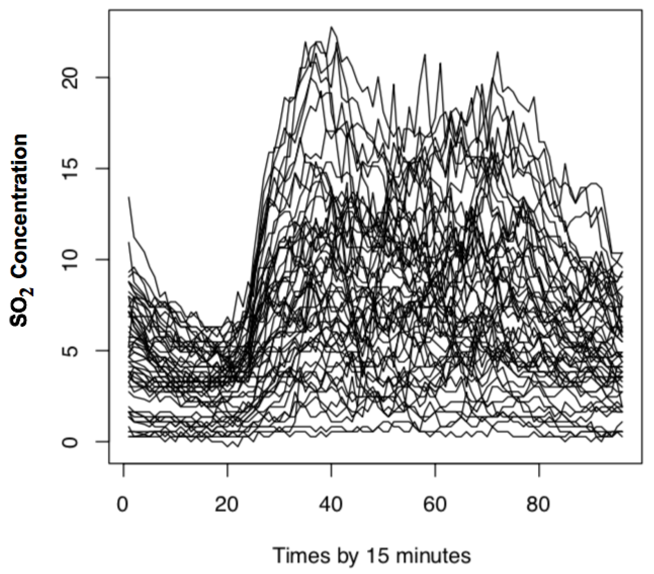
In addition to the first example that highlights the importance of the kNN approach over the classical kernel method, we emphasize in this second example the superiority of the local linear approach over the local constant approach. For this purpose, we consider a time series from air quality data. The importance of this kind of data is motivated by the fact that the air quality has a potential environmental impact on the quality of life of humans and the health of animals. In particular, it is well documented that exposures to ground ozone levels for a period of 1–8 h reduce various pulmonary functions and affect the respiratory tract’s tissues. Thus, the approximation of the excessive level of ozone concentration is a primordial subject in environmental sciences. In this example, we focus on the air quality in Westminster city in London. The time-series data was collected at the Marylebone road site by real-time monitoring. Let us point out that our study can be used to model the distribution of the ozone given the daily curves of the ocher polluting gases (carbon monoxide, carbon dioxide, Sulphur dioxide, Nitrogen dioxide, Nitric oxide, etc.). However, for the sake of shortness, we focus on two important indices of air quality that are the sulfur dioxide (SO2) and the ozone concentration (O3). It is well known that (SO2) increases the stratospheric ozone concentrations when it reacts with ultraviolet rays. This example’s data is more complicated than the first example because the time series data is observed on a more fine grid. The link to this data is also provided in the “Data Availability Statement” section. Precisely, unlike the yearly curve of the first example, here, the ozone concentration is hourly observed, and the sulfur dioxide is observed by time-gride equal to 15 min. Thus, this kind of time series data is more adapted for our functional approach. It worth noting that the use of functional statistical models in this type of environmental studies has been widely studied by many authors FDA (see, for example, Quintela-del-Río and Francisco-Fernández (2011) to cite a few). In this example, we aim to analyze the relationship between the SO2 and the O3 in Westminster city using the SCMI predictive region. Specifically, we wish to predict the total ozone one day before using the daily curve of SO2. Formally, we observe 364 days of air quality data in Marylebone road station, where is the daily curve of SO2 in day i and the total ozone of the day . A sample of the functional regressors is shown in Figure 4. It concerns the daily curves of the sulphur dioxide observed by a time gride equal to 15 min, and the value of SO2 in the vertical axis was measured in term of micrograms per cubic meter (μg/m3).
We highlight the importance of the local linear approach over the classical local constant one for this actual data set. In particular, the local linear approach reduces the bias term of the local constant. So, we shall quantify this gain in practice. To do this, we compare the SCMI of both estimators: the kNN-LLM and the kNN-CKM. In addition, we keep the same strategies as those used in the first example to select the parameters involved in the estimator. More precisely, we use the quadratic kernel on , the PCA metric, and the criterion to choose the number of neighborhood k.
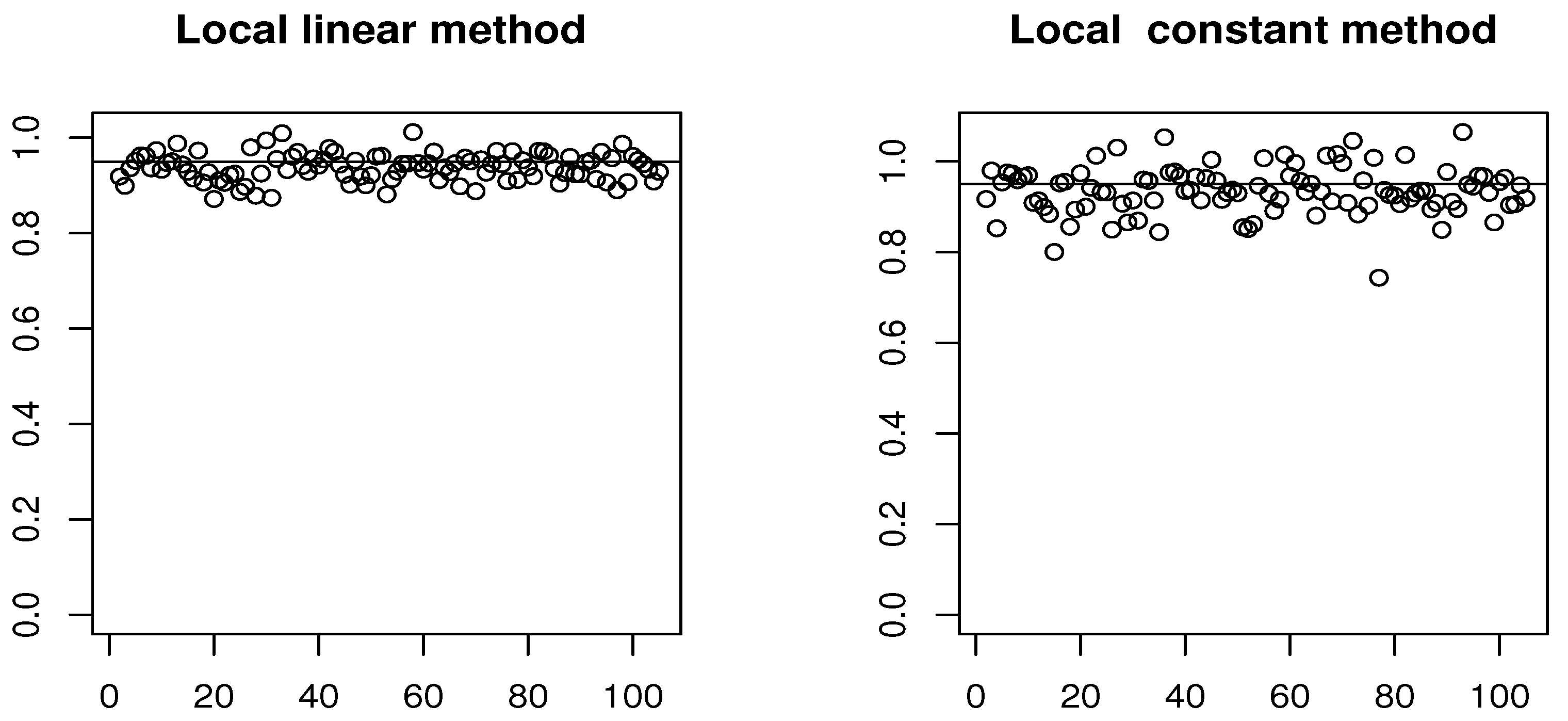
For our comparison purpose, we put and split the data sample randomly into two parts: the learning sample (260 observations) and the test sample (104 observations). Finally, we examine both estimators’ efficiency by Probability Coverage (PC), which is the main criterion to evaluate the predictive regions. In particular, we draw in the Figure 5, the PC of the testing sample obtained by the two estimation methods.
We see that the local linear estimation has better performance than that based on the local constant method. Of course, this conclusion is not surprising since it reflects the superiority of the local linear approach in the bias term. Undoubtedly, we can say that the kNN-LLM keeps its advantages over the local constant method in the functional time series case.
6. Conclusions and Perspectives
The present contribution investigates the problem of the local linear estimation of the distribution function of real random variable conditioning on a functional covariate. The main novelty of this paper is to construct an estimator using the double kernels kNN estimation procedure. The main feature of the built estimator is its smoothing property. The latter improves the estimators’ flexibility and broadens the scope of application of the conditional distribution estimation. From a theoretical point of view, the estimator’s asymptotic property is established under a more general domain called the functional time series case. Specifically, the dependence setting is modeled through the strong mixing condition. It is well known that this kind of dependency covers an extensive class of usual processes, including the AR process, ARMA process, Gaussian process, Markov process, Linear process, and m-dependent, among others. From a practical point of view, we have illustrated the constructed estimator’s feasibility using real data. The computational study shows that the proposed estimator has a good behavior as prediction models. It improves the prediction by the classical kernel method in both single predictions or by predictive region. This statement confirms the superiority of the kNN local linear estimation over the standard kernel one. Moreover, in addition to this considerable development of the nonparametric functional conditional models, the present contribution opens numerous future research tracks in nonparametric functional data analysis. For instance, it will be very interesting to establish the asymptotic normality of the proposed estimator, to consider the weak functional time series case or incomplete functional time series data case. On the other hand, the robustness of the predictors is a crucial issue in functional data analysis. At this stage, studying the consistency of the kNN-LLM estimator of the robust regression in functional time series is an important prospect of the present contribution. It permits the reduction of the sensitivity of the kNN approach to the noisy data, missing values, and the presence of outliers.
Supplementary Materials
The following are available online at https://www.mdpi.com/article/10.3390/math9101102/s1.
Author Contributions
Writing—review & editing, I.M.A., Z.C.E., A.L. and M.R. The authors contributed equally to this work. All authors have read and agreed to the published version of the manuscript.
Funding
This research was funded by the Deanship of Scientific Research at King Khalid University through the Research Groups Program under grant number R.G.P. 2/82/42.
Institutional Review Board Statement
Not applicable.
Informed Consent Statement
Not applicable.
Data Availability Statement
The first data that used in the first example is available at https://www.met.hu/en/eghajlat/magyarorszag_eghajlata/eghajlati_adatsorok/Debrecen/adatok/napi_adatok/index.php (accessed on 30 March 2021). The second data that used in the second example is available at https://www.airqualityengland.co.uk/site/data?site_id=MY1 (accessed on 30 March 2021).
Acknowledgments
The authors would like to thank the anonymous reviewers for their valuable comments and suggestions which improved the quality of this article substantially. They thank and extend their appreciation to the Deanship of Scientific Research at King Khalid University for funding this work.
Conflicts of Interest
The authors declare no conflict of interest.
References
- Fan, J.; Gijbels, I. Local Polynomial Modelling and Its Applications; Chapman & Hall: London, UK, 1996. [Google Scholar]
- Baìllo, A.; Grané, A. Local linear regression for functional predictor and scalar response. J. Multivar. Anal. 2009, 100, 102–111. [Google Scholar] [CrossRef] [Green Version]
- Barrientos-Marin, J.; Ferraty, F.; Vieu, P. Locally Modelled Regression and Functional Data. J. Nonparametr. Stat. 2010, 22, 617–632. [Google Scholar] [CrossRef]
- Berlinet, A.; Elamine, A.; Mas, A. Local linear regression for functional data. Ann. Inst. Stat. Math. 2011, 63, 1047–1075. [Google Scholar] [CrossRef] [Green Version]
- Zhou, Z.; Lin, Z. Asymptotic normality of locally modelled regression estimator for functional data. J. Nonparametr. Stat. 2016, 28, 116–131. [Google Scholar] [CrossRef]
- Laksaci, A.; Rachdi, M.; Rahmani, S. Spatial modelization: Local linear estimation of the conditional distribution for functional data. Spatial Stat. 2013, 6, 1–23. [Google Scholar] [CrossRef]
- Burba, F.; Ferraty, F.; Vieu, P. k-nearest neighbor method in functional non-parametric regression. J. Nonparametr. Stat. 2009, 21, 453–469. [Google Scholar] [CrossRef]
- Laloë, T. A k-nearest neighbor approach for functional regression. Stat. Probab. Lett. 2008, 78, 1189–1193. [Google Scholar] [CrossRef] [Green Version]
- Kudraszow, N.; Vieu, P. Uniform consistency of kNN regressors for functional variables. Stat. Probab. Lett. 2013, 83, 1863–1870. [Google Scholar] [CrossRef]
- Kara, L.Z.; Laksaci, A.; Rachdi, M.; Vieu, P. Data-driven kNN estimation in nonparametric functional data analysis. J. Multivar. Anal. 2017, 153, 176–188. [Google Scholar] [CrossRef]
- Chikr-Elmezouar, Z.; Almanjahie, I.M.; Laksaci, A.; Rachdi, M. FDA: Strong consistency of the kNN local linear estimation of the functional conditional density and mode. J. Nonparametr. Stat. 2019, 31, 175–195. [Google Scholar] [CrossRef]
- Bachir, A.; Almanjahie, I.M.; Attouch, M.K. The k Nearest Neighbors Estimator of the M-Regression in Functional Statistics. CMC-Comput. Mater. Continua 2020, 65, 2049–2064. [Google Scholar] [CrossRef]
- Laksaci, A.; Ould-Said, E.; Rachdi, M. Uniform consistency in number of neighbors of the kNN estimator of the conditional quantile model. Metrika 2021, 1–17. [Google Scholar] [CrossRef]
- Rachdi, M.; Laksaci, A.; Kaid, Z.; Benchiha, A.; Al-Awadhi, F.A. k-nearest neighbors local linear regression for functional and missing data at random. Stat. Neerl. 2021, 75, 42–65. [Google Scholar] [CrossRef]
- Almanjahie, I.M.; Alahmari, W.M.; Laksaci, A.; Rachdi, M. Computational aspects of the kNN local linear smoothing for some conditional models in high dimensional statistics. Commun. Stat. Simul. Comput. 2021. [Google Scholar] [CrossRef]
- Almanjahie, I.M.; Elmezouar, Z.C.; Laksaci, A.; Rachdi, M. kNN local linear estimation of the conditional cumulative distribution function: Dependent functional data case. Comptes Rendus Math. 2018, 356, 1036–1039. [Google Scholar] [CrossRef]
- Ferraty, F.; Vieu, P. Nonparametric Functional Data Analysis. Theory and Practice; Springer Series in Statistics; Springer: New York, NY, USA, 2006. [Google Scholar]
- Yao, Q.; Tong, H. On initial-condition sensitivity and prediction in nonlinear stochastic systems. Bull. Int. Stat. Inst. 1995, 50, 395–412. [Google Scholar]
- DeGooijer, J.G.; Gannoun, A. Nonparametric conditional predictive regions for time series. Comput. Stat. Data Anal. 2000, 33, 259–275. [Google Scholar] [CrossRef]
Figure 1.
Monthly mean temperature.

Figure 2.
Mean temperature by year.

Figure 3.
Prediction and confidence bands by SCMI-rule.

Figure 4.
The daily curves of the SO2.

Figure 5.
The PC of LLM (on the left) and the PC of LCM (on the right).


Table 1.
The average of the length of the SCMI for kNN-LLM and CKM estimators.
| kNN-LLM Estimator | CKM Estimator | |
|---|---|---|
| Average of the length of the SCMI | 1.23 | 2.07 |
Publisher’s Note: MDPI stays neutral with regard to jurisdictional claims in published maps and institutional affiliations. |
© 2021 by the authors. Licensee MDPI, Basel, Switzerland. This article is an open access article distributed under the terms and conditions of the Creative Commons Attribution (CC BY) license (https://creativecommons.org/licenses/by/4.0/).
Share and Cite
MDPI and ACS Style
Almanjahie, I.M.; Elmezouar, Z.C.; Laksaci, A.; Rachdi, M. Smooth kNN Local Linear Estimation of the Conditional Distribution Function. Mathematics 2021, 9, 1102. https://doi.org/10.3390/math9101102
AMA Style
Almanjahie IM, Elmezouar ZC, Laksaci A, Rachdi M. Smooth kNN Local Linear Estimation of the Conditional Distribution Function. Mathematics. 2021; 9(10):1102. https://doi.org/10.3390/math9101102
Chicago/Turabian StyleAlmanjahie, Ibrahim M., Zouaoui Chikr Elmezouar, Ali Laksaci, and Mustapha Rachdi. 2021. "Smooth kNN Local Linear Estimation of the Conditional Distribution Function" Mathematics 9, no. 10: 1102. https://doi.org/10.3390/math9101102
Note that from the first issue of 2016, this journal uses article numbers instead of page numbers. See further details here.