A Fourth Order Symplectic and Conjugate-Symplectic Extension of the Midpoint and Trapezoidal Methods

Abstract

The paper presents fourth order Runge–Kutta methods derived from symmetric Hermite–Obreshkov schemes by suitably approximating the involved higher derivatives. In particular, starting from the multi-derivative extension of the midpoint method we have obtained a new symmetric implicit Runge–Kutta method of order four, for the numerical solution of first-order differential equations. The new method is symplectic and is suitable for the solution of both initial and boundary value Hamiltonian problems. Moreover, starting from the conjugate class of multi-derivative trapezoidal schemes, we have derived a new method that is conjugate to the new symplectic method.

1. Introduction

In the present work, we will consider a suitable modification of multi-derivative one-step methods derived in [1] for the numerical solution of first order differential equations

$$y^{\prime }\left(t\right)=f\left(y\left(t\right)\right),t\in [t_0,T],$$

(1)

with sufficiently regular vector field $f:{\mathbb{R}}^m\to {\mathbb{R}}^m$, subject to initial conditions $y\left(t_0\right)=y_0$, or boundary conditions $g(y\left(t_0\right),y\left(T\right))=0$. The methods we are going to introduce are especially suited for the long time simulation of canonical Hamiltonian problems

$$y^{\prime }=J\nabla H\left(y\right),y\left(t_0\right)=y_0\in {\mathbb{R}}^{2m},$$

(2)

with

$$y=\left(\begin{array}{c}q\\ p\end{array}\right),q,p\in {\mathbb{R}}^m,J=\left(\begin{array}{cc}\hfill O& \hfill I\\ \hfill -I& \hfill O\end{array}\right),$$

(3)

where q and p are the generalized coordinates and conjugate momenta, $H:{\mathbb{R}}^{2m}\to \mathbb{R}$ is the Hamiltonian function and I stands for the identity matrix of dimension m. The investigation of numerical methods for integrating differential equations such as (2) forms a branch of numerical analysis called Geometric Integration. Problem (2) admits the Hamiltonian function $H\left(y\right)$ as a first integral, namely $H\left(y\left(t\right)\right)=H\left(y_0\right)$ for $t\ge t_0$. It may admit additional constant of motions bringing important physical properties of the system that general-purpose codes would fail to reproduce in a long time simulation. Rather than focusing on the control of the accuracy in a given time interval of finite length, geometric integrators aim at reproducing the correct global behavior of the trajectory in the phase space, trying to retain the geometric features of the system itself. We refer the reader to the monographs [2,3,4] for the fundamental theory on the numerical treatment of conservative problems. Examples of the relevant role of geometric integration in several application areas may be found in the review papers [5,6,7] and references therein.

In [8,9] we analyzed two classes of one step symmetric Hermite–Obreshkov schemes with interesting symplectic properties and in [1] we focused on the symplectic properties of two families of multi-derivative high-order one-step methods which contains the well-known implicit midpoint and trapezoidal methods as seed formulae. Here, we consider a proper discretization of the Lie derivative appearing in these formulae, to define Runge–Kutta schemes with geometric properties. In the following, $y_1={\Phi }_h\left(y_0\right)$ denotes a generic one-step method of order $p>0$ that provides the numerical solution of (2) with stepsize of integration $h>0$. We recall a few definitions and properties which are relevant for our analysis. The one-step method ${\Phi }_h$ is called:

-

symplectic, if its Jacobian matrix is symplectic, that is

$$\frac{\partial {\Phi }_h{\left(y\right)}^{\top }}{\partial y}J\frac{\partial {\Phi }_h\left(y\right)}{\partial y}=J,\mathrm{for} \mathrm{all}y\in {\mathbb{R}}^{2m}.$$

(4)

-

conjugate-symplectic, if it is topologically conjugate to a symplectic method $y_1={\Psi }_h\left(y_0\right)$, which means that a global change of coordinates ${\chi }_h\left(y\right)=y+O\left(h\right)$ exists such that

$${\Phi }_h={\chi }_h\circ {\Psi }_h\circ {\chi }_h^{-1}.$$

(5)

-

conjugate-symplectic up to order r, if there exists a global change of coordinates

${\chi }_h\left(y\right)=y+O\left(h^p\right)$ such that (5) holds true, with the map ${\Psi }_h$ satisfying

$$\frac{\partial {\Psi }_h{\left(y\right)}^{\top }}{\partial y}J\frac{\partial {\Psi }_h\left(y\right)}{\partial y}=J+O\left(h^{p+r+1}\right).$$

(6)

A symplectic method inherits relevant properties of the flow associated with a canonical Hamiltonian problem such as volume preservation of closed surfaces in the phase space under time evolution. For a detailed analysis of symplectic Runge–Kutta methods, see the monographs [2,3,4]. Further relevant features are the conservation of quadratic first integrals, and near conservation of the Hamiltonian function over exponentially long times ([4], page 366).

Conjugate-symplecticity leave these properties essentially unchanged (see [4] page 222 and [10]). In fact, from (5) we have

$$y_n={\Phi }_h^n\left(y_0\right)={({\chi }_h\circ {\Psi }_h\circ {\chi }_h^{-1})}^n\left(y_0\right)={\chi }_h\circ {\Psi }_h^n\circ {\chi }_h^{-1}\left(y_0\right).$$

The third property listed above is clearly a relaxation of conjugate-symplecticity. In this case, the method ${\Phi }_h\left(y\right)$ nearly conserves all quadratic first integrals and the Hamiltonian function over time intervals of length $O\left(h^{-r}\right)$ (see [11]).

The starting point of our investigation is the class of Hermite–Obreshkov (HO) linear multistep methods [12].

$$\sum _{i=0}^k{\alpha }_i{y}_{n+i}=\sum _{j=1}^l{h}^j\sum _{i=0}^k{\beta }_{ji}{y}_{n+i}^{\left(j\right)}.$$

(7)

Here $y_{n+i}^{\left(j\right)}$ denotes an approximation to the j-th derivative of the solution $y\left(t\right)$ at $t_{n+i}$, with $t_{n+i}=t_n+ih$ and is defined as

$$y_n^{\left(j\right)}:=D_{j-1}f\left(y_n\right),j=1,2,\cdots ,l.$$

(8)

For a given integer $k\ge 0$ and $u\in {\mathbb{R}}^m$, $D_k\left(f\left(u\right)\right)$ is the k-th order Lie derivative of the vector field f, defined as the k-th time derivative of $f\left(y\right(t\left)\right)$ formally computed at $y\left(t\right)=u,$ assuming that $y\left(t\right)$ satisfies the differential equation in (1) ($D_0=I$ is the identity operator). We have used the subscript to define this operator to avoid confusion with the same order classical derivative operator denoted by $D^k$. Of course, the two operators take the same values when applied to the projection of the true solution $y\left(t\right)$ on the mesh points but, in general, they will differ. Recently, we have introduced and analyzed four different one step ($k=1$) HO methods:

-

Euler–Maclaurin methods: higher derivative collocation methods deriving their name from the well-known Euler–Maclaurin integration formula. In [9] it has been shown that these integrators are conjugate-symplectic up to order $p+2$.

-

BS Hermite–Obreshkov methods: based on a special subclass of Hermite–Obreshkov methods which admit a continuous spline extension [8], these formulae are a multi-derivative generalization of the BS linear multistep methods derived in [13] and generalized in the field of quasi-interpolation in [14,15,16]. In [8] it has been shown that the BS Hermite–Obreshkov methods are conjugate-symplectic up to order $p+2$.

-

multi-derivative midpoint and trapezoidal methods: generalizations of the classical midpoint and trapezoidal methods, these formulae are derived by a combination of the implicit Taylor and the explicit Taylor expansion up to a given order [1]. The multi-derivative midpoint (MDMP) and trapezoidal (MDTR) methods are conjugate-symplectic up to order $p+2$.

The analysis of these classes of multi-derivative methods has been also motivated by the possibility of computing the derivative efficiently, by exploiting the Infinity Computer arithmetic as described in [17,18,19]. In fact, the analytical computation of the j-th derivative $y^{\left(j\right)}$ involves a tensor of order j, which evidently heavily affects the computational cost associated with the implementation of the method. In this respect, the use of the Infinity Computer is able to accurately evaluate $y^{\left(j\right)}\left(z\right)$ without requiring its explicit expression in terms of the derivatives of f. In this paper, we consider the more natural approach that uses finite differences to approximate the Lie derivatives appearing in a given multi-derivative formula.

Since a certain degree of freedom is allowed in the choice of the derivative discretization stepsize, it turns out that the final full discretized formula may exhibit more favorable geometric properties with respect to the original one. This is the case for two special methods in the classes we are going to introduce: they form a pair of symplectic and conjugate-symplectic Runge–Kutta integrators that originate from the midpoint method and its conjugate-symplectic counterpart, namely the trapezoidal methods. To the best of our knowledge, no couple of symplectic and conjugate-symplectic Runge–Kutta methods of order higher than two has been devised up to now, so their existence constitutes the core result of the paper.

In addition, we introduce and analyze a new technique for solving the nonlinear systems emerging from the implementation of the methods. It consists of a block-diagonal variant of the simplified Newton scheme which requires, at each integration step, a single Jacobian evaluation of the vector field and a single LU factorization of a matrix having the same size of the continuous problem. Moreover, the diagonal structure of the linear systems involved in the iterative procedure, makes it suitable for a parallel implementation. A comparison of the new integrators with other existing symplectic integrators in terms of their efficiency is a delicate question and will not be addressed here.

The paper is organized as follows. In Section 2 we illustrate the multi-derivative fourth-order extensions of the midpoint and trapezoidal methods, while their modifications obtained by approximating the Lie derivatives are introduced in Section 3 and Section 4 respectively. Section 5 analyzes the above-mentioned nonlinear systems solver needed to advance the solution in time. Some numerical illustrations are presented in Section 6. Finally, Section 7 contains some concluding remarks.

2. MDMP and MDTR Methods

The multi-derivative generalization of the midpoint (MP) and trapezoidal (TR) methods we are interested in is easily obtained via a standard Taylor approach by exploiting the property that such schemes may be viewed as composition of the Implicit (IE) and Explicit Euler (EE) methods, in direct and reverse order, applied on half the integration time-step:

MP = EE ∘ IE:

$$y_{n+1}=y_n+hf\left(\frac{y_n+y_{n+1}}{2}\right)⟺\left\{\begin{array}{c}{\displaystyle y_{n+1/2}=y_n+\frac{h}{2}f\left(y_{n+1/2}\right),}\hfill \\ {\displaystyle y_{n+1}=y_{n+1/2}+\frac{h}{2}f\left(y_{n+1/2}\right),}\hfill \end{array}\right.$$

TR = IE ∘ EE:

$$y_{n+1}=y_n+\frac{h}{2}\left(f\left(y_n\right)+f\left(y_{n+1}\right)\right)$$

We focus on the two conjugate classes of the MDMP and MDTR methods of order four. By denoting as ET4 (IT4) the explicit (implicit) Taylor method of order four we have that

MDMP4 =  ET4 ∘ IT4:

${\displaystyle y_{n+1}=y_n+hf\left(y_{n+1/2}\right)+\frac{h^3}{24}{D}_{2}f\left(y_{n+1/2}\right),}$

⟺$\left\{\begin{array}{c}{\displaystyle y_{n+1/2}=y_n+\frac{h}{2}f\left(y_{n+1/2}\right)-\frac{h^2}{8}{D}_{1}f\left(y_{n+1/2}\right)+\frac{h^3}{48}{D}_{2}f\left(y_{n+1/2}\right),}\hfill \\ {\displaystyle y_{n+1}=y_{n+1/2}+\frac{h}{2}f\left(y_{n+1/2}\right)+\frac{h^2}{8}{D}_{1}f\left(y_{n+1/2}\right)+\frac{h^3}{48}{D}_{2}f\left(y_{n+1/2}\right),}\hfill \end{array}\right.$

MDTR4 =  IT4 ∘ ET4:

${\displaystyle y_{n+1}=y_n+\frac{h}{2}\left(f\left(y_{n+1}\right)+f\left(y_n\right)\right)-\frac{h^2}{8}\left(D_{1}f\left(y_{n+1}\right)-D_{1}f\left(y_n\right)\right)+\frac{h^3}{48}\left(D_{2}f\left(y_{n+1}\right)+D_{2}f\left(y_n\right)\right),}$

⟺$\left\{\begin{array}{c}{\displaystyle y_{n+1/2}=y_n+\frac{h}{2}f\left(y_n\right)+\frac{h^2}{8}{D}_{1}f\left(y_n\right)+\frac{h^3}{48}{D}_{2}f\left(y_n\right),}\hfill \\ {\displaystyle y_{n+1}=y_{n+1/2}+\frac{h}{2}f\left(y_{n+1}\right)-\frac{h^2}{8}{D}_{1}f\left(y_{n+1}\right)+\frac{h^3}{48}{D}_{2}f\left(y_{n+1}\right).}\hfill \end{array}\right.$

Here we introduce and analyze two families of methods depending on a real parameter, which are derived by approximating the Lie derivative appearing in the formulae above by means of suitable difference schemes. These latter are defined with the aid of auxiliary local steps that will be exploited for this purpose. We observe that two Lie derivatives used in the MDMP4 and MDTR4 methods are multiplied respectively by $h^2$ and $h^3$, so we shall approximate them by means of symmetric difference schemes of order at least two to preserve the symmetry and order properties of the original methods.

For the same reason, the formulae used to approximate the solution in the additional local steps should also be at least of order two. In particular, they take the form of implicit or explicit methods of order two so that the symmetry condition of the resulting method is preserved. In the next two sections we introduce these new fourth-order methods.

3. Approximated MDMP

In this section, we show two generalizations of the MDMP4 method. All the presented extensions are based on the computation of two local approximations of the solution in the two additional steps

$$t_{n+1/2-\alpha }=t_{n+1/2}-\alpha hand{t}_{n+1/2+\alpha }=t_{n+1/2}+\alpha h,$$

where $\alpha$ is a real positive parameter. In all the cases to approximate the first and second Lie derivatives we use the following standard finite differences schemes of order two:

$$\begin{array}{cc}\hfill {\widehat{D}}_1{f}_{n+1/2}=& {\displaystyle \frac{f\left(y_{n+1/2+\alpha }\right)-f\left(y_{n+1/2-\alpha }\right)}{2\alpha h},}\hfill \\ \hfill {\widehat{D}}_2{f}_{n+1/2}=& {\displaystyle \frac{f\left(y_{n+1/2+\alpha }\right)-2f\left(y_{n+1/2}\right)+f\left(y_{n+1/2-\alpha }\right)}{{\alpha }^2{h}^2}.}\hfill \end{array}$$

(9)

3.1. Computation of the Additional Stages Using the Standard Explicit RK Method of Order 2

Let us approximate the value of $y\left(t\right)$ at $t_{n+1/2-\alpha }$ and $t_{n+1/2+\alpha }$ by using the explicit Runge–Kutta method of order 2 backward and forward, starting at $t_{n+1/2}$. The obtained values are used to compute the approximation of the derivatives using the central differences formulas in (9). The resulting method is

$$\begin{array}{c}\hfill \begin{array}{cc}\hfill Y_{n+\frac{1}{2}-\alpha }=& y_{n+\frac{1}{2}}-h\alpha f_{n+\frac{1}{2}},\hfill \\ \hfill y_{n+\frac{1}{2}-\alpha }=& {\displaystyle y_{n+\frac{1}{2}}-\frac{h\alpha }{2}(F_{n+\frac{1}{2}-\alpha }+f_{n+\frac{1}{2}}),}\hfill \\ \hfill Y_{n+\frac{1}{2}+\alpha }=& y_{n+\frac{1}{2}}+h\alpha f_{n+\frac{1}{2}},\hfill \\ \hfill y_{n+\frac{1}{2}+\alpha }=& {\displaystyle y_{n+\frac{1}{2}}+\frac{h\alpha }{2}(F_{n+\frac{1}{2}+\alpha }+f_{n+\frac{1}{2}}),}\hfill \\ \hfill y_{n+\frac{1}{2}}=& {\displaystyle y_n+\frac{h}{2}{f}_{n+\frac{1}{2}}-\frac{h^2}{8}{\widehat{D}}_1{f}_{n+\frac{1}{2}}+\frac{h^3}{48}{\widehat{D}}_2{f}_{n+\frac{1}{2}},}\hfill \\ \hfill y_{n+1}=& {\displaystyle y_n+h{f}_{n+\frac{1}{2}}+\frac{h^3}{24}{\widehat{D}}^2{f}_{n+\frac{1}{2}}}\hfill \end{array}\end{array}$$

where $f_{n+\frac{1}{2}}=f(y_{n+\frac{1}{2}})$, $Y_{n+\frac{1}{2}\pm \alpha }$ are the stages of the two Runge–Kutta steps and $F_{n+\frac{1}{2}\pm \alpha }=f(Y_{n+\frac{1}{2}\pm \alpha })$. We call this method AMDMP4_RK2. Written as a Runge–Kutta scheme the method is described by the tableau

$$\begin{array}{cc}c& A\\ & b\end{array}\equiv \begin{array}{cccccc}1/2-\alpha & \frac{1}{16\alpha }+b_1& -\frac{\alpha }{2}& -\frac{\alpha }{2}+b_3/2& 0& -\frac{1}{16\alpha }+b_5\\ 1/2-\alpha & \frac{1}{16\alpha }+b_1& 0& -\alpha +b_3/2& 0& -\frac{1}{16\alpha }+b_5\\ 1/2& \frac{1}{16\alpha }+b_1& 0& b_3/2& 0& -\frac{1}{16\alpha }+b_5\\ 1/2+\alpha & \frac{1}{16\alpha }+b_1& 0& \alpha +b_3/2& 0& -\frac{1}{16\alpha }+b_5\\ 1/2+\alpha & \frac{1}{16\alpha }+b_1& 0& \frac{\alpha }{2}+b_3/2& \frac{\alpha }{2}& -\frac{1}{16\alpha }+b_5\\ & b_1& 0& b_3& 0& b_5\end{array}$$

where $b_1=b_5=1/\left(24{\alpha }^2\right)$ and $b_3=1-1/\left(12{\alpha }^2\right)$. The fourth-order conditions have been checked by exploiting the formulas in [12] (Table 2.2 p. 148). Applying the method to the scalar linear test problem $y^{\prime }=\lambda y$, we obtain the recurrence relation $y_{n+1}=R\left(h\lambda \right)y_n$, where $R\left(z\right)=1+z{b}^{\top }{(I_5-zA)}^{-1}e$ is the stability function ($I_5$ denotes the identity matrix of size 5 and $e={(1,1,1,1,1)}^{\top }$). For a general introduction to the linear stability theory of Runge–Kutta schemes, we refer to [20] (chapter IV.3) and [21]. It turns out that, for AMDMP4_RK2 methods, the stability function actually does not depend on the parameter $\alpha$. Setting, as usual, $q=h\lambda$, it takes the form

$$R\left(q\right)=\frac{P\left(q\right)}{Q\left(q\right)}=\frac{q^3+6q^2+24q+48}{-q^3+6q^2-24q+48}.$$

Since $P\left(q\right)=Q(-q)$, we get $\left|R\right(q\left)\right|=1$ on the imaginary axis and since the poles of $R\left(q\right)$ have a positive real part, the maximum modulus principle shows that all the formulae in the family are precisely A-stable, that is its domain of absolute stability coincides with ${\mathbb{C}}^{-}$.

In comparison with the original MDMP method we see that the computational cost for the implementation of the new formulae decreases, because we just need to add the computation of the two explicit steps in the nonlinear iteration.

3.2. Approximation of the Derivative Using the Trapezoidal Scheme of Order 2

The second family of methods is derived by approximating the Lie derivatives with the aid of the backward and forward trapezoidal schemes. The resulting method is

$$\begin{array}{ccc}\hfill y_{n+\frac{1}{2}-\alpha }& =& {\displaystyle y_{n+\frac{1}{2}}-\frac{h\alpha }{2}(f_{n+\frac{1}{2}-\alpha }+f_{n+\frac{1}{2}})}\hfill \\ \hfill y_{n+\frac{1}{2}+\alpha }& =& {\displaystyle y_{n+\frac{1}{2}}+\frac{h\alpha }{2}(f_{n+\frac{1}{2}+\alpha }+f_{n+\frac{1}{2}})}\hfill \\ \hfill y_{n+\frac{1}{2}}& =& {\displaystyle y_n+\frac{h}{2}{f}_{n+\frac{1}{2}}-\frac{h^2}{8}{\widehat{D}}_1{f}_{n+\frac{1}{2}}+\frac{h^3}{48}{\widehat{D}}_2{f}_{n+\frac{1}{2}},}\hfill \\ \hfill y_{n+1}& =& {\displaystyle y_n+h{f}_{n+\frac{1}{2}}+\frac{h^3}{24}{\widehat{D}}_2{f}_{n+\frac{1}{2}}}\hfill \end{array}$$

Written as a Runge–Kutta scheme we have the following tableau

$$\begin{array}{cccc}1/2-\alpha & -\frac{\alpha }{2}+\frac{1}{16\alpha }+\frac{1}{48{\alpha }^2}& -\frac{\alpha }{2}+\frac{1}{2}-\frac{1}{24{\alpha }^2}& \frac{1}{16\alpha }+\frac{1}{48{\alpha }^2}\\ 1/2& \frac{1}{16\alpha }+\frac{1}{48{\alpha }^2}& \frac{1}{2}-\frac{1}{24{\alpha }^2}& -\frac{1}{16\alpha }+\frac{1}{48{\alpha }^2}\\ 1/2+\alpha & \frac{1}{16\alpha }+\frac{1}{48{\alpha }^2}& -\frac{\alpha }{2}+\frac{1}{2}+\frac{1}{24{\alpha }^2}& \frac{\alpha }{2}+\frac{1}{16\alpha }+\frac{1}{48{\alpha }^2}\\ & \frac{1}{24{\alpha }^2}& 1-\frac{1}{12{\alpha }^2}& \frac{1}{24{\alpha }^2}\end{array}$$

(10)

and it is easy to check that its order is four. More interestingly, within this family we may discover a new fourth-order symplectic Runge–Kutta formula.

Theorem 1.

The Runge–Kutta scheme defined by the tableau (10) is A-stable for $\alpha <1/\sqrt{6}$ and it is symplectic if we choose $\alpha =\sqrt{2}/4$.

Proof. 

The stability function $R\left(q\right)$ is equal to the following rational function:

$$R\left(q\right)=\frac{P\left(q\right)}{Q\left(q\right)}=\frac{-(6{\alpha }^2-1)q^3-(12{\alpha }^2-6)q^2+24q+48}{(6{\alpha }^2-1)q^3-(12{\alpha }^2-6)q^2-24q+48},$$

(11)

from which $P\left(q\right)=Q(-q)$ and hence $\left|R\right(q\left)\right|=1$ on the imaginary axis. In order to impose that the poles of R lie in the right-half of the complex plane, we can apply the Routh–Hurwitz stability criterion to $Q(-q)=P\left(q\right)$. A direct computation then leads to the condition $\alpha <1/\sqrt{6}$ for the roots of $P\left(q\right)$ to have negative real part. Consequently, for these values of $\alpha$, the method is precisely A-stable. A sufficient condition for symplecticity (see [4] (Theorem 4.3) or [22]) is $b_i{a}_{ij}+b_j{a}_{ji}-b_i{b}_j=0,i,j=1,2,3$. It turns out that this condition is satisfied only if we choose $\alpha =\sqrt{2}/4$. □

The new symplectic RK method is

$$\begin{array}{cccc}1/2-\frac{\sqrt{2}}{4}& \frac{1}{6}& \frac{1}{6}-\frac{\sqrt{2}}{8}& \frac{1}{6}-\frac{\sqrt{2}}{8}\\ 1/2& \frac{1}{6}+\frac{\sqrt{2}}{8}& \frac{1}{6}& \frac{1}{6}-\frac{\sqrt{2}}{4}\\ 1/2+\frac{\sqrt{2}}{4}& \frac{1}{6}+\frac{\sqrt{2}}{8}& \frac{1}{6}+\frac{\sqrt{2}}{8}& \frac{1}{6}\\ & \frac{1}{3}& \frac{1}{3}& \frac{1}{3}\end{array}$$

(12)

Symplectic Runge–Kutta schemes with three stages and order four are already known in the literature, see for example [23]. The method (12) has the special property of being defined as the composition of two formulae: this suggests that the method obtained by the reverse composition is conjugate to (12), and thus we get a couple of symplectic/conjugate-symplectic Runge–Kutta schemes that extend to the fourth-order the well-known couple formed by the midpoint and trapezoidal methods. The conjugate-symplectic method associated with (12) is introduced in the next section.

4. Approximated MDTR4 Methods

In this section, we devise two classes of methods obtained by approximating the Lie derivatives appearing in the MDTR4 formulae: each method in these families are conjugate to the corresponding one derived in Section 3. All the generalizations are based on the computation of two local approximations of the solution in two additional steps depending on a positive parameter $\alpha$. This time, the new additional steps are

$$t_{n+1-\alpha }=t_{n+1}-\alpha hand{t}_{n+1+\alpha }=t_{n+1}+\alpha h.$$

To approximate the Lie derivatives, we use the same finite differences schemes of order two used in (9) for the AMDMP4 methods:

$$\begin{array}{cc}\hfill {\widehat{D}}_1{f}_{n+1}=& {\displaystyle \frac{f\left(y_{n+1+\alpha }\right)-f\left(y_{n+1-\alpha }\right)}{2\alpha h}}\end{array}$$

(13)

$$\begin{array}{cc}\hfill {\widehat{D}}_2{f}_{n+1}=& {\displaystyle \frac{f\left(y_{n+1+\alpha }\right)-2f\left(y_{n+1}\right)+f\left(y_{n+1-\alpha }\right)}{{\alpha }^2{h}^2}}\end{array}$$

(14)

4.1. Approximation of the Derivative Using the Standard Explicit RK Method of Order 2

As in the previous section, the first family of methods is derived by employing the second order explicit Runge–Kutta methods to approximate the solution in the two extra abscissae $t_{n+1-\alpha }$ and $t_{n+1+\alpha }$. We get

$$\begin{array}{ccc}\hfill Y_{n+1-\alpha }& =& {\displaystyle y_{n+1}-h\alpha f_{n+1},}\hfill \\ \hfill y_{n+1-\alpha }& =& {\displaystyle y_{n+1}-h\frac{\alpha }{2}(F_{n+1-\alpha }+f_{n+1}),}\hfill \\ \hfill Y_{n+1+\alpha }& =& {\displaystyle y_{n+1}+h\alpha f_{n+1},}\hfill \\ \hfill y_{n+1+\alpha }& =& {\displaystyle y_{n+1}+h\frac{\alpha }{2}(F_{n+1+\alpha }+f_{n+1}),}\hfill \\ \hfill y_{n+1}& =& {\displaystyle y_n+\frac{h}{2}(f_n+f_{n+1})-\frac{h^2}{8}\left({\widehat{D}}_1{f}_n-{\widehat{D}}_1{f}_{n+1}\right)}\hfill \\ \hfill & & {\displaystyle +\frac{h^3}{48}\left({\widehat{D}}_2{f}_n+{\widehat{D}}_2{f}_{n+1}\right).}\hfill \end{array}$$

(15)

This method, denoted by AMDTR4_RK2, is symmetric and has order four. Written as a Runge–Kutta scheme, it has $s=10$ stages and the following tableau:

$$\begin{array}{ccccccccccc}-\alpha & 0& -\frac{\alpha }{2}& -\frac{\alpha }{2}& 0& 0& 0& 0& 0& 0& 0\\ -\alpha & 0& 0& -\alpha & 0& 0& 0& 0& 0& 0& 0\\ 0& 0& 0& 0& 0& 0& 0& 0& 0& 0& 0\\ \alpha & 0& 0& \alpha & 0& 0& 0& 0& 0& 0& 0\\ \alpha & 0& 0& \frac{\alpha }{2}& \frac{\alpha }{2}& 0& 0& 0& 0& 0& 0\\ 1-\alpha & b_1& 0& b_3& 0& b_5& b_6& -\frac{\alpha }{2}& -\frac{\alpha }{2}+b_8& 0& b_{10}\\ 1-\alpha & b_1& 0& b_3& 0& b_5& b_6& 0& -\alpha +b_8& 0& b_{10}\\ 1& b_1& 0& b_3& 0& b_5& b_6& 0& b_8& 0& b_{10}\\ 1+\alpha & b_1& 0& b_3& 0& b_5& b_6& 0& \alpha +b_8& 0& b_{10}\\ 1+\alpha & b_1& 0& b_3& 0& b_5& b_6& 0& \frac{\alpha }{2}+b_8& \frac{\alpha }{2}& b_{10}\\ & b_1& 0& b_3& 0& b_5& b_6& 0& b_8& 0& b_{10}\end{array}$$

where the non null weights $b_i$ are

$$b_1=b_{10}=-\frac{1}{16\alpha }+\frac{1}{48{\alpha }^2},b_3=b_8=\frac{1}{2}-\frac{1}{24{\alpha }^2},b_5=b_6=\frac{1}{16\alpha }+\frac{1}{48{\alpha }^2}.$$

The coefficient matrix A has a block structure with many vanishing elements. The AMDTR4_RK2 scheme may be also cast as a parameterized implicit Runge–Kutta (PIRK) method having the general form

$$\begin{array}{ccc}\hfill Y_i& =& v_i{y}_n+(1-v_i)y_{n+1}+h\sum _{j=1}^s{x}_{i,j}f(t_n+c_{j}h,Y_j),i=1,\cdots s\hfill \\ \hfill y_{n+1}& =& y_n+h\sum _{j=1}^s{b}_{j}f(t_n+c_{j}h,Y_j),\hfill \end{array}$$

and represented by the tableau

$$\begin{array}{ccc}c& v& X\\ & & b^T\end{array}$$

with $c_i=v_i+{\sum }_{j=1}^s{x}_{i,j}$. Notice that a PIRK is equivalent to a RK with $A=X+v{b}^T$. Order results for this class of methods are reported in [24], where the special subclass of mono-implicit Runge–Kutta (MIRK) methods is analyzed. The MIRK class has been investigated by many authors since it has the interesting feature that the matrix X is strictly lower triangular. In this form, the method AMPTR_RK2 has the following tableau:

$$\begin{array}{cccccccccccc}-\alpha & 0& 0& -\frac{\alpha }{2}& -\frac{\alpha }{2}& 0& 0& 0& 0& 0& 0& 0\\ -\alpha & 0& 0& 0& -\alpha & 0& 0& 0& 0& 0& 0& 0\\ 0& 0& 0& 0& 0& 0& 0& 0& 0& 0& 0& 0\\ \alpha & 0& 0& 0& \alpha & 0& 0& 0& 0& 0& 0& 0\\ \alpha & 0& 0& 0& \frac{\alpha }{2}& \frac{\alpha }{2}& 0& 0& 0& 0& 0& 0\\ 1-\alpha & 1& 0& 0& 0& 0& 0& 0& -\frac{\alpha }{2}& -\frac{\alpha }{2}& 0& 0\\ 1-\alpha & 1& 0& 0& 0& 0& 0& 0& 0& -\alpha & 0& 0\\ 1& 0& b_1& 0& b_3& 0& b_5& b_6& 0& b_8& 0& b_{10}\\ 1+\alpha & 1& 0& 0& 0& 0& 0& 0& 0& \alpha & 0& 0\\ 1+\alpha & 1& 0& 0& 0& 0& 0& 0& 0& \frac{\alpha }{2}& \frac{\alpha }{2}& 0\\ & & b_1& 0& b_3& 0& b_5& b_6& 0& b_8& 0& b_{10}\end{array}$$

Separating the block involving $t_n$ with the one involving $t_{n+1}$ leads to another representation of the AMDTR4_RK2 method as a one-step block method with $s=5$ stages, namely

$$T{Z}_{n+1}=e_3{e}_3^T{Z}_n+h{e}_3{d}^T{G}_n+hB{G}_{n+1},$$

where (see (15))

$$Z_n=\left(\begin{array}{c}{Y}_{n-\alpha }\\ y_{n-\alpha }\\ y_n\\ Y_{n+\alpha }\\ y_{n+\alpha }\end{array}\right),G_n=\left(\begin{array}{c}f\left(Y_{n-\alpha }\right)\\ f\left(y_{n-\alpha }\right)\\ f\left(y_n\right)\\ f\left(Y_{n+\alpha }\right)\\ f\left(y_{n+\alpha }\right)\end{array}\right),d=\left(\begin{array}{c}{b}_1\\ 0\\ b_3\\ 0\\ b_5\end{array}\right),e_3=\left(\begin{array}{c}0\\ 0\\ 1\\ 0\\ 0\end{array}\right),$$

$$T=\left(\begin{array}{ccccc}1& 0& -1& 0& 0\\ 0& 1& -1& 0& 0\\ 0& 0& 1& 0& 0\\ 0& 0& -1& 1& 0\\ 0& 0& -1& 0& 1\end{array}\right),B=\left(\begin{array}{ccccc}0& -\alpha /2& -\alpha /2& 0& 0\\ 0& 0& -\alpha & 0& 0\\ b_6& 0& b_8& 0& b_{10}\\ 0& 0& \alpha & 0& 0\\ 0& 0& \alpha /2& \alpha /2& 0\end{array}\right),$$

with T, B, d and $e_3$ used as linear operators, to simplify the notation avoiding the explicit use of the Kronecker products. This latter expression, besides being more compact than the previous ones, leads to a better implementation in terms of computational efficiency.

Applied to the test equation $y^{\prime }=\lambda y$, the AMDTR4_RK2 method defines the following recursion:

$$Y_{n+1}={(I-q{T}^{-1}B)}^{-1}{T}^{-1}(e_3{e}_3^T+q{e}_3{d}^T)Y_n=G\left(q\right)Y_n$$

where $q=h\lambda$. The matrix $G\left(q\right)$ has four eigenvalues equal to zero and one equal to the following rational function:

$$R\left(q\right)=\frac{P\left(q\right)}{Q\left(q\right)}=\frac{q^3+6q^2+24q+48}{-q^3+6q^2-24q+48}.$$

Again we see that $P\left(q\right)=Q(-q)$ and a direct computation shows that $R\left(q\right)$ is analytic in the left-half of the complex plane, so the method is precisely A-stable.

4.2. Approximation of the Derivative Using the Trapezoidal Scheme of Order 2

Approximating the solution in the additional points by the trapezoidal scheme yields

$$\begin{array}{ccc}\hfill y_{n+1-\alpha }& =& y_{n+1}-h\frac{\alpha }{2}(f_{n+1-\alpha }+f_{n+1}),\hfill \\ \hfill y_{n+1+\alpha }& =& y_{n+1}+h\frac{\alpha }{2}(\frac{1}{3}{f}_{n+1}+f_{n+1+\alpha }),\hfill \\ \hfill y_{n+1}& =& y_n+\frac{h}{2}(f_{n+1}+f_n)-\frac{h^2}{8}\left({\widehat{D}}_1{f}_n-{\widehat{D}}_1{f}_{n+1}\right)+\frac{h^3}{48}\left({\widehat{D}}_2{f}_n+{\widehat{D}}_2{f}_{n+1}\right).\hfill \end{array}$$

These formulae, denoted by AMDTR4_TR2, have order 4. Choosing $\alpha =\sqrt{2}/4$ we get a method which is conjugate to the corresponding method AMDMP4_TR2 defined at (12). In block form, this method assumes the following shape:

$$T{Z}_{n+1}=e_2{e}_2^T{Z}_n+h{e}_2{d}^T{G}_n+hB{G}_{n+1},$$

where

$$Z_n=\left(\begin{array}{c}{y}_{n-\alpha }\\ y_n\\ y_{n+\alpha }\end{array}\right),G_n=\left(\begin{array}{c}f\left(y_{n-\alpha }\right)\\ f\left(y_n\right)\\ f\left(y_{n+\alpha }\right)\end{array}\right),d=\left(\begin{array}{c}-\frac{1}{16\alpha }+\frac{1}{48{\alpha }^2}\\ \frac{1}{2}-\frac{1}{24{\alpha }^2}\\ \frac{1}{16\alpha }+\frac{1}{48{\alpha }^2}\end{array}\right),e_2=\left(\begin{array}{c}0\\ 1\\ 0\end{array}\right),$$

$$T=\left(\begin{array}{ccc}1& -1& 0\\ 0& 1& 0\\ 0& -1& 1\end{array}\right),B=\left(\begin{array}{ccc}-\alpha /2& -\alpha /2& 0\\ d_3& d_2& d_1\\ 0& \alpha /2& \alpha /2\end{array}\right),$$

with T, B, d and $e_2$ used as linear operators.

Applied to the test equation $y^{\prime }=\lambda y$ we have that the solution is defined by the following recursion:

$$Y_{n+1}={(I-q{T}^{-1}B)}^{-1}{T}^{-1}(e_2{e}_2^T+q{e}_2{d}^T)Y_n=G\left(q\right)Y_n$$

where $q=h\lambda$. The matrix $G\left(q\right)$ has two vanishing eigenvalues and one eigenvalue equal to the same rational function defined at (11). From Theorem 1, it then follows that the formulae are precisely A-stable for $\alpha <1/\sqrt{6}$.

5. Solution of the Nonlinear Systems

In order to optimize the computational cost associated with each method derived in the previous sections, we employ a suitable modified Newton scheme to solve the nonlinear systems emerging from their implementation. In particular, we approximate the Jacobian matrix with a diagonal block-matrix with constant diagonal blocks. The derived iterative scheme for the AMDMP methods is the following

$$\left(I_s\otimes I-\frac{h}{\beta }(I_s\otimes J)\right)\left(Y_{n+1}^{r+1}-Y_{n+1}^r\right)=-\left(Y_{n+1}^r-e\otimes y_n\right)+h(A\otimes I)f\left(Y_{n+1}^r\right)$$

(16)

where $A\in {\mathbb{R}}^{s\times s}$ denotes the coefficient matrix of the method (s is the number of stages), $J\in {\mathbb{R}}^{m\times m}$ is the Jacobian matrix of the vector field f, evaluated at $(t_n,y_n)$, $y_n$ is the solution computed at the previous step $t_n$, $\beta$ is a positive parameter, while $I_s$ and I stand for the identity matrices of size s and m respectively.

Theorem 2.

The nonlinear iteration scheme (16) applied to the AMDMP4_TR2 method for the solution of the test equations $y^{\prime }=\lambda y$ is convergent for $Re\left(q\right)<0$ if the spectral radius ρ of the matrix $\beta A-I$ is less then one. When $\rho >1$, the method converges if

$$\left|q\right|\in \left\{\frac{\beta cos\theta +\sqrt{{\beta }^2({cos}^2\theta +{\rho }^2-1)}}{{\rho }^2-1},-\frac{\pi }{2}\le \theta \le \frac{\pi }{2}\right\}$$

Proof. 

The scheme (16) applied to the test equation reduces to the following iteration:

$$Y_{n+1}^{r+1}=q{(1-\frac{q}{\beta })}^{-1}(A-\frac{1}{\beta }I)Y_{n+1}^r+{(1-\frac{q}{\beta })}^{-1}e\otimes y_n.$$

The eigenvalues of the iteration matrix are the eigenvalues of the matrix $\beta A-I$ scaled by $q/(\beta -q)$. It is straightforward to check that if $\rho <1$ the method is convergent when $Re\left(q\right)<0$. The region of convergence when $\rho >1$ is computed by imposing that $\rho |q/\beta -q)|<1$. □

Corollary 1.

The nonlinear iteration scheme (16) with $0<\beta \le 7$ applied to the AMDMP4_TR2 with $\alpha =\sqrt{2}/4$ for the solution of the test equations $y^{\prime }=\lambda y$, converges if $\Re \left(\lambda \right)<0$. The minimum value at ∞ is $\approx 0.5637$ and is attained choosing $\beta \approx 4.6721$.

Proof. 

The eigenvalues of the matrix $(\beta A-I)$ have absolute value less than one for $0<\beta \le 7$ with minimum value $\approx 0.5637$ for $\beta \approx 4.6721$. □

Observe that the iterative scheme (16) only requires one LU factorization of size m and the solution of the nonlinear systems could be easily performed in parallel. Depending on the structure of the problem, this is surely an interesting approach for solving nonlinear equations.

A similar argument may be applied to the solution of the nonlinear systems arising from the implementation of the AMDTR4_TR2 methods. The details are omitted for the sake of brevity.

6. Numerical Illustrations

In the present section, we compare the behavior of the newly-derived formulae with that of the original multi-derivative methods. These integrators have been applied to the well-known Kepler problem, a super-integrable Hamiltonian system that describes the motion of two bodies subject to Newton’s law of gravitation (see, for example [25]). By setting the origin of the coordinate system on one of the two bodies, the Hamiltonian function takes the form

$$H(q,p)=\frac{1}{2}(p_1^2+p_2^2)-\frac{1}{\sqrt{q_1^2+q_2^2}}.$$

In particular, taking as initial conditions

$$q_1\left(0\right)=1-e,q_2\left(0\right)=0,p_1\left(0\right)=0,p_2\left(0\right)=\sqrt{\frac{1+e}{1-e}},$$

the trajectory describes an ellipse with eccentricity e in the $q_1-q_2$ plane and is periodic with period $T=2\pi$. Besides the total energy H, further relevant first integrals are the angular momentum

$$M(q,p)=q_1{p}_2-q_2{p}_1,$$

and the Lenz vector $A={(A_1,A_2,A_3)}^{\top }$, whose components are

$$A_1(q,p)=p_{2}M(q,p)-\frac{q_1}{{\left|\right|q\left|\right|}_2},A_2(q,p)=-p_{1}M(q,p)-\frac{q_2}{{\left|\right|q\left|\right|}_2},A_3(q,p)=0.$$

Of the four first integrals $H,M,A_1$ and $A_2$, only three are independent so, for example, $A_1$ can be neglected.

Having set $e=0.6$ and $h=T/200$, we integrated the problem over ${10}^3$ periods and computed the error $\parallel y_n-y_0{\parallel }_1$ in the solution at specific times multiples of the period T, that is for $n=200k$, with $k=1,2,\cdots$. All computations have been carried out on an Intel i7 quad-core CPU with 16GB of RAM, running MATLAB R2020b.

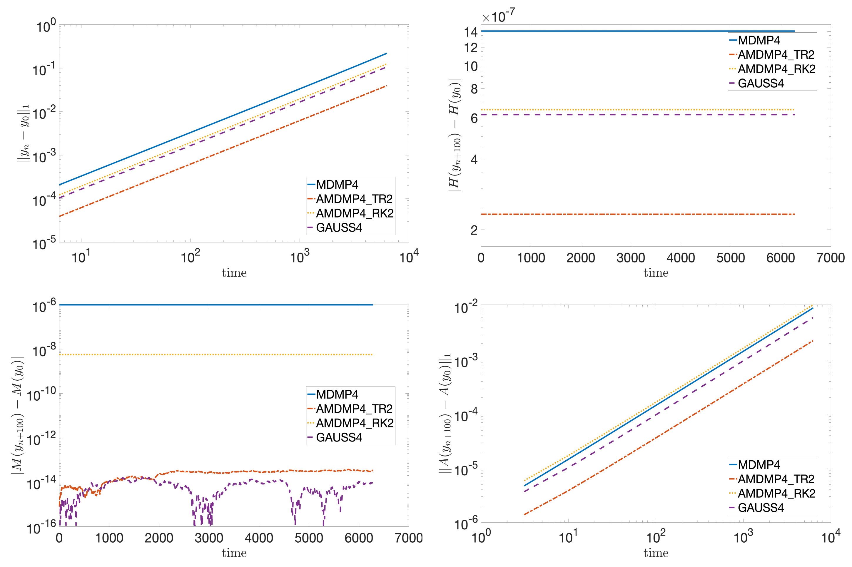
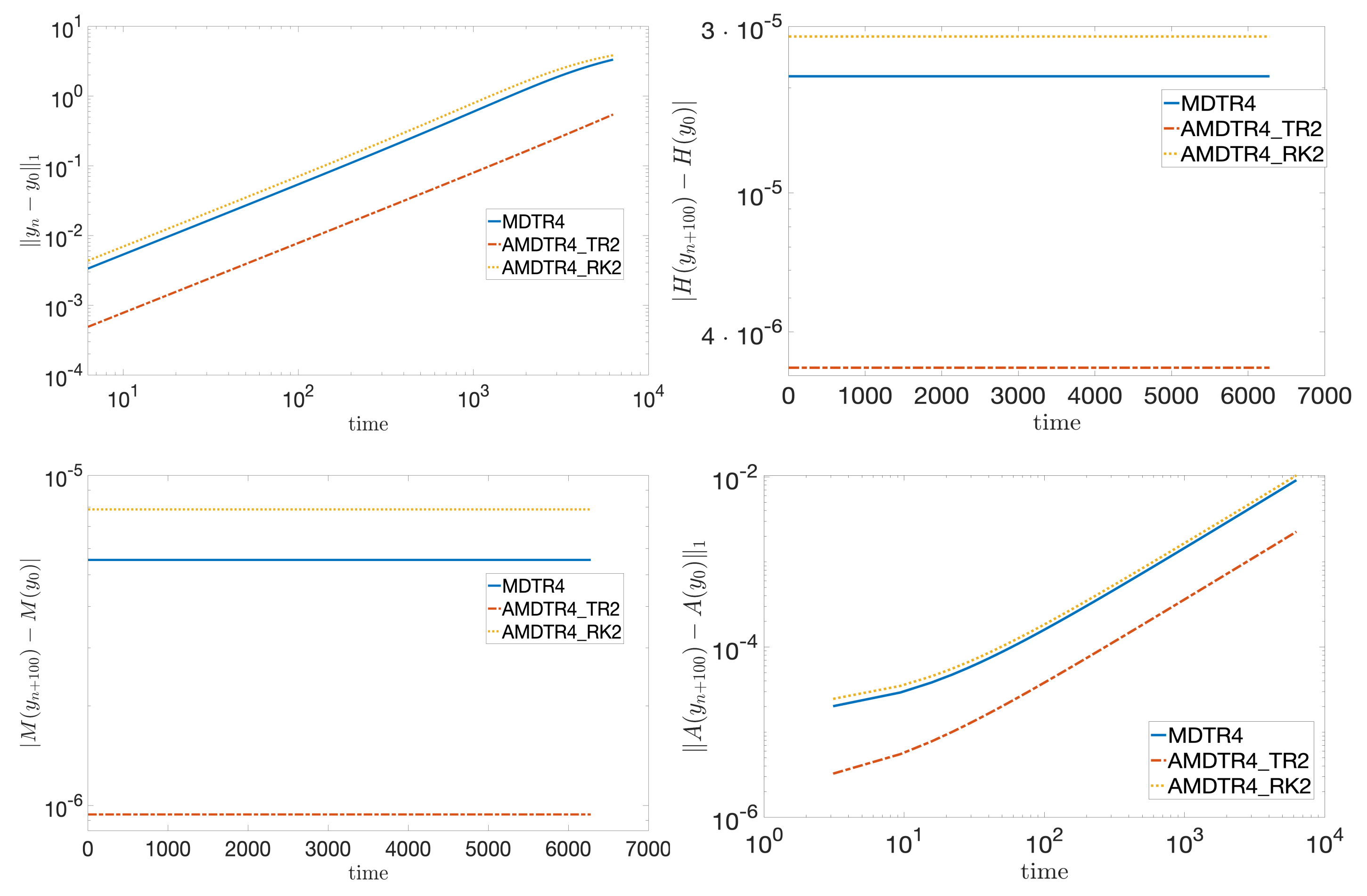
Figure 1 and Figure 2 report the results for the considered methods. On the top-left picture is the absolute error of the numerical solution; the top-right picture shows the error in the Hamiltonian function; the error in the angular momentum is drawn in the bottom-left picture, while the bottom-right picture concerns the error in the second component of the Lenz vector. To get more insights on the performance and conservation properties of the symplectic AMDMP_TR2 formula, in Figure 1 we also report the results for the Gauss method of order four. We observe that, to make the pictures more readable, the errors in the first integrals are computed at the midpoint of each period, that is at the points $t_{n+100}$.

As is expected from a symplectic or a conjugate-symplectic integrator, we can see a linear drift in the error $\parallel y_n-y_0{\parallel }_1$ as the time increases. The same linear growth is experienced in the Lenz invariant. The conjugate-symplectic AMDMP_TR2 scheme assures near conservation of the Hamiltonian function and angular momentum. This latter quadratic invariant is precisely conserved (up to machine precision) by the symplectic schemes.

In

Table 1. Error in the angular momentum for the methods in the MDMP family.

	AMDMP
	TR2		RK2
$\mathbf{\alpha }$	$\frac{\sqrt{\mathbf{2}}}{\mathbf{4}\mathbf{\gamma }}$	$\frac{\sqrt{\mathbf{2}}\mathbf{\gamma }}{\mathbf{4}}$	$\frac{\mathbf{1}}{\mathbf{2}\mathbf{\gamma }}$
$\gamma$
1	$5.32\times {10}^{-15}$	$5.32\times {10}^{-15}$	$3.60\times {10}^{-7}$
$1.2$	$4.86\times {10}^{-6}$	$6.97\times {10}^{-6}$	$4.65\times {10}^{-6}$
$1.4$	$7.81\times {10}^{-6}$	$1.51\times {10}^{-5}$	$7.67\times {10}^{-6}$
$1.6$	$9.72\times {10}^{-6}$	$2.45\times {10}^{-5}$	$9.62\times {10}^{-6}$
$1.8$	$1.10\times {10}^{-5}$	$3.51\times {10}^{-5}$	$1.09\times {10}^{-5}$
$2.0$	$1.19\times {10}^{-5}$	$4.68\times {10}^{-5}$	$1.19\times {10}^{-5}$
$3.0$	$1.42\times {10}^{-5}$	$1.20\times {10}^{-4}$	$1.41\times {10}^{-5}$
	MDMP
	$1.60\times {10}^{-5}$

and

Table 2. Error in the angular momentum for the methods in the MDTR family, computed at the midpoints $t_{n+1/2}$. As reference value, we use the one computed at $t_{1/2}$.

	AMDTR				AMDTR Midpoints
	TR2		RK2		TR2		RK2
$\mathbf{\alpha }$	$\frac{\sqrt{\mathbf{2}}}{\mathbf{4}\mathbf{\gamma }}$	$\frac{\sqrt{\mathbf{2}}\mathbf{\gamma }}{\mathbf{4}}$	$\frac{\mathbf{1}}{\mathbf{2}\mathbf{\gamma }}$	$\mathbf{\alpha }$	$\frac{\sqrt{\mathbf{2}}}{\mathbf{4}\mathbf{\gamma }}$	$\frac{\sqrt{\mathbf{2}}\mathbf{\gamma }}{\mathbf{4}}$	$\frac{\mathbf{1}}{\mathbf{2}\mathbf{\gamma }}$
$\gamma$				$\gamma$
1	$1.55\times {10}^{-5}$	$1.55\times {10}^{-5}$	$1.32\times {10}^{-4}$	1	$5.88\times {10}^{-15}$	$5.88\times {10}^{-15}$	$3.40\times {10}^{-7}$
$1.2$	$1.89\times {10}^{-5}$	$6.46\times {10}^{-5}$	$6.34\times {10}^{-5}$	$1.2$	$4.73\times {10}^{-6}$	$6.78\times {10}^{-6}$	$4.52\times {10}^{-6}$
$1.4$	$3.96\times {10}^{-5}$	$1.22\times {10}^{-4}$	$2.13\times {10}^{-5}$	$1.4$	$7.59\times {10}^{-6}$	$1.47\times {10}^{-5}$	$7.45\times {10}^{-6}$
$1.6$	$5.31\times {10}^{-5}$	$1.88\times {10}^{-4}$	$6.87\times {10}^{-6}$	$1.6$	$9.45\times {10}^{-6}$	$2.38\times {10}^{-5}$	$9.35\times {10}^{-6}$
$1.8$	$6.23\times {10}^{-5}$	$2.63\times {10}^{-4}$	$2.55\times {10}^{-5}$	$1.8$	$1.07\times {10}^{-5}$	$3.41\times {10}^{-5}$	$1.06\times {10}^{-5}$
$2.0$	$6.90\times {10}^{-5}$	$3.45\times {10}^{-4}$	$3.91\times {10}^{-5}$	$2.0$	$1.16\times {10}^{-5}$	$4.55\times {10}^{-5}$	$1.15\times {10}^{-5}$
$3.0$	$8.47\times {10}^{-5}$	$8.69\times {10}^{-4}$	$7.14\times {10}^{-5}$	$3.0$	$1.38\times {10}^{-5}$	$1.17\times {10}^{-4}$	$1.37\times {10}^{-5}$
	MDTR				MDTR midpoints
	$9.730\times {10}^{-5}$				$1.55\times {10}^{-5}$

, we compare the symplectic and conjugate-symplectic formulae with other methods in the same families, in terms of their ability in conserving the angular momentum. To this end, the value of $\alpha =\sqrt{2}/4$ that generates the symplectic and conjugate-symplectic schemes has been scaled by factors $\gamma$ and $1/\gamma$, for a few values of $\gamma >0$. We observe that when $\gamma$ increases, the errors related to the decreasing values of $\alpha$ approach the value of the corresponding multi-derivative methods. As was expected, the angular momentum is exactly preserved by the symplectic scheme while the value attained at $t_{1/2}=t_0+h/2$ is exactly preserved by the conjugate-symplectic one.

To show the convergence properties of the diagonal nonlinear iteration (16) introduced in Section 5, we solved the problem over ${10}^2$ periods with sepsize $h=T/N$, choosing $\beta =4.6721$ (see Corollary 1). For comparison purposes, we also consider the use of the standard simplified Newton scheme defined by approximating the Jacobian matrix with $(I_3\otimes I-hA\otimes J)$ (compare with (16)).

In

Table 3. Convergence rate and mean number of approximated Newton iterations for the AMDMP4_TR2 method with $\alpha =\sqrt{2}/4$.

N	Error	Order	Iterations Per Step (Simplified Newton)	Iterations Per Step (Scheme (16))
100	$4.6981\times {10}^{-2}$		$5.18$	$9.32$
200	$3.0275\times {10}^{-3}$	$3.95$	$4.52$	$8.12$
400	$1.9059\times {10}^{-4}$	$3.98$	$4.21$	$7.24$
800	$1.1933\times {10}^{-5}$	$3.99$	$3.83$	$6.48$

we show for the AMDMP4_TR2 method with $\alpha =\sqrt{2}/4$ the absolute error, the computed convergence rate and the mean number of iterations needed to reach the convergence up to machine precision for the two techniques. The scheme defined by the block-diagonal matrix requires around $1.7$ more iterations to attain convergence, but the cost of the Jacobian factorization decreases from 27 m³ to m³. The execution times of the two algorithms for this problem are essentially equivalent, since the computation of the factorization is a built-in optimized function in Matlab so the differences do not consistently show up.

7. Conclusions

Starting from two fourth-order multi-derivative extensions of the midpoint and trapezoidal formulae, we have derived one-parameter families of standard Runge–Kutta methods through the approximation of the first and second-order Lie derivatives by means of suitable finite difference schemes. The resulting formulae retain the order and the symmetry properties of the original methods while, avoiding the use of Lie derivatives, their implementation turns out to be simplified. More interestingly, for a specific choice of the parameter, a symplectic/conjugate-symplectic pair of methods may be detected. This novel result generalizes to order four the well-known conjugacy relationship between the midpoint and the trapezoidal methods. Concerning the implementation of the methods, a block-diagonal version of the simplified Newton scheme has been employed. The iteration requires, at each step, a single Jacobian evaluation of the vector field and a LU factorization of a matrix having the same size of the continuous problem and, interestingly, may be executed in parallel.

References

- Iavernaro, F.; Mazzia, F. On conjugate-symplecticity properties of a multi-derivative extension of the midpoint and trapezoidal methods. Rend. Semin. Mat. 2018, 76, 123–134. [Google Scholar]
- Feng, K.; Quin, M. Symplectic Geometric Algorithms for Hamiltonian Systems; Springer, Zhejiang Publishing United Group Zhejiang Science and Technology Publishing House: Zhejiang, China, 2010. [Google Scholar]
- Sanz-Serna, J.; Calvo, M. Numerical Hamiltonian Problems; Chapman & Hall: London, UK, 1994. [Google Scholar]
- Hairer, E.; Lubich, C.; Wanner, G. Geometric Numerical Integration. Structure-Preserving Algorithms for Ordinary Differential Equations, 2nd ed.; Springer: Berlin, Germany, 2006. [Google Scholar]
- Budd, C.J.; Piggott, M.D. Geometric Integration and its Applications. In Handbook of Numerical Analysis; North-Holland Publishing Co.: Amsterdam, The Netherlands, 2003; Volume 11, pp. 35–139. [Google Scholar]
- McLachlan, R.I. Perspectives on geometric numerical integration. J. R. Soc. N. Z. 2019, 49, 114–125. [Google Scholar] [CrossRef]
- Diele, F.; Marangi, C. Geometric numerical integration in ecological modelling. Mathematics 2020, 8, 25. [Google Scholar] [CrossRef] [Green Version]
- Mazzia, F.; Sestini, A. On a class of conjugate symplectic Hermite-Obreshkov one-step methods with continuous spline extension. Axioms 2018, 7, 58. [Google Scholar] [CrossRef] [Green Version]
- Iavernaro, F.; Mazzia, F.; Mukhametzhanov, M.; Sergeyev, Y. Conjugate-symplecticity properties of Euler–Maclaurin methods and their implementation on the Infinity Computer. Appl. Numer. Math. 2020, 155, 58–72. [Google Scholar] [CrossRef] [Green Version]
- Hairer, E. Conjugate-symplecticity of linear multistep methods. J. Comput. Math. 2008, 26, 657–659. [Google Scholar]
- Hairer, E.; Zbinden, C.J. On conjugate symplecticity of B-series integrators. IMA J. Numer. Anal. 2013, 33, 57–79. [Google Scholar] [CrossRef] [Green Version]
- Hairer, E.; Nørsett, S.P.; Wanner, G. Solving Ordinary Differential Equations. I. Nonstiff Problems, 2nd ed.; Springer Series in Computational Mathematics; Springer: Berlin, Germany, 1993. [Google Scholar]
- Mazzia, F.; Sestini, A.; Trigiante, D. The continuous extension of the B-spline linear multistep methods for BVPs on non-uniform meshes. Appl. Numer. Math. 2009, 59, 723–738. [Google Scholar] [CrossRef]
- Mazzia, F.; Sestini, A. The BS class of Hermite spline quasi-interpolants on nonuniform knot distributions. BIT Numer. Math. 2009, 49, 611–628. [Google Scholar] [CrossRef]
- Mazzia, F.; Sestini, A. Quadrature formulas descending from BS Hermite spline quasi-interpolation. J. Comput. Appl. Math. 2012, 236, 4105–4118. [Google Scholar] [CrossRef]
- Bracco, C.; Giannelli, C.; Mazzia, F.; Sestini, A. Bivariate hierarchical Hermite spline quasi-interpolation. BIT Numer. Math. 2016, 56, 1165–1188. [Google Scholar] [CrossRef] [Green Version]
- Sergeyev, Y.; Mukhametzhanov, M.; Mazzia, F.; Iavernaro, F.; Amodio, P. Numerical methods for solving initial value problems on the infinity computer. Int. J. Unconv. Comput. 2016, 12, 3–23. [Google Scholar]
- Iavernaro, F.; Mazzia, F. Symplecticity properties of Euler-Maclaurin methods. AIP Conf. Proc. 2018, 1978. [Google Scholar] [CrossRef]
- Iavernaro, F.; Mazzia, F.; Mukhametzhanov, M.; Sergeyev, Y. Computation of higher order Lie derivatives on the Infinity Computer. J. Comput. Appl. Math. 2021, 383. [Google Scholar] [CrossRef]
- Hairer, E.; Wanner, G. Solving Ordinary Differential Equations II. Stiff and Differential Algebraic Problems, 2nd ed.; Springer: Berlin, Germany, 1996. [Google Scholar]
- Butcher, J. Runge-Kutta methods. Scholarpedia 2007, 2, 3147, revision #91735. [Google Scholar] [CrossRef]
- Sanz-Serna, J. Runge-Kutta schemes for Hamiltonian systems. BIT 1988, 28, 877–883. [Google Scholar] [CrossRef]
- Maeda, S. Certain types of Runge-Kutta-type formulas and reproduction of orbits of linear systems. Electron. Commun. Jpn. 1991, 74, 98–104. [Google Scholar] [CrossRef]
- Burrage, K.; Chipman, F.; Muir, P. Order Results for Mono-Implicit Runge–Kutta Methods. SIAM J. Numer. Anal. 1994, 31, 876–891. [Google Scholar] [CrossRef] [Green Version]
- Brugnano, L.; Iavernaro, F. Line Integral Methods for Conservative Problems; Monographs and Research Notes in Mathematics; CRC Press: Boca Raton, FL, USA, 2016. [Google Scholar]
Figure 1.
Results for the fourth-order MDMP (solid lines), Gauss (dashed lines), AMDMP_TR2 (dash-dotted lines) and AMDMP_R2 (dotted lines) methods applied to the Kepler problem computed at each period.
Figure 2.
Results for the fourth-order MDTR (solid lines), Gauss (dashed lines), AMDTR_TR2 (dash-dotted lines) and AMDTR_R2 (dotted lines) methods applied to the Kepler problem computed at each period.